Applicability of the low-cost OPC-N3 optical particle counter for microphysical measurements of fog

Low-cost devices for particulate matter measurements are characterised by small dimensions and a light weight. This advantage makes them ideal for UAV measurements, where those parameters are crucial. However, they also have some issues. The values of particulate matter from low-cost optical particle counters can be biased by high ambient humidity. In this article, we evaluate the low-cost Alphasense OPC-N3 optical particle counter for measuring the microphysical properties of fog. This study aimed to show that OPC-N3 not only registers aerosols or humidified aerosols but also registers fog droplets.

The study was carried out on the rooftop of the Institute of Geophysics, University of Warsaw, Poland, during autumn–winter 2021. To validate the results, the data from OPC-N3 were compared with the data obtained from the reference instrument, the Oxford Lasers VisiSize D30. VisiSize D30 is a shadowgraph device able to register photos of individual droplets.

Considering the effective radius of droplets, it is possible to differentiate low-visibility situations between fog conditions (which are not hazardous for people) from haze events, when highly polluted air can cause health risks to people.

The compared microphysical properties were liquid water content (LWC), number concentration (N_c), effective radius r_eff and statistical moments of radius. The Pearson correlation coefficient between both devices for LWC was 0.92, N_c was 0.95 and r_eff was 0.63. Overall, these results suggest good compliance between instruments. However, the OPC-N3 has to be corrected regarding professional equipment.

1 Introduction

Fog is defined as a layer of water droplets (or ice crystals) near the Earth's surface, which reduces visibility to below 1 km (Gultepe, 2007). Depending on the cause which helps in forming it, there are different types of fog, e.g. radiation fog, advection fog and valley fog. Radiation fog forms in the evening when the heat absorbed by the Earth's surface during the day is radiated into the air. The air near the ground cools down when the air reaches saturation, and the first layer of fog forms. The fog phenomenon can affect the small scale (valley fog) to the regional scale of the whole country.

Fog is a dangerous phenomenon for transport safety (Gultepe et al., 2015; Bartok et al., 2012), which causes increased road accidents as well as downtime of aircraft flights. This phenomenon affects the carriage of goods by land, air and maritime transport, causing financial losses similar to those caused by extreme weather events (Kulkarni et al., 2019; Price et al., 2018).

The research by Vautard et al. (2009) shows that fog in Europe has decreased significantly in the last 30 years. This can be the outcome of an increase in air temperature (Klemm and Lin, 2016). However, the fog decrease trend is spatially and temporally correlated with a negative trend in sulfur dioxide emissions, indicating that air quality policies significantly impact fog occurrence (Vautard et al., 2009).

Particulate matter (PM) is a suspension of solid or liquid particles in the air, such as dust or soot. Aerosol is a critical component that contributes to fog formation. A decrease in PM can cause changes in fog occurrence or its microphysics. Fog is generated with relatively low super-saturation (SS). Mazoyer et al. (2022) showed that the amount of activated aerosol depends more on the aerosol size than its chemical composition. Numerical simulations conducted by Tsai et al. (2021) show that for urban aerosols, a higher density of aerosols resulted in more but smaller droplets and increased liquid water content (LWC). The effect of urban aerosols was more pronounced near the surface, where the aerosols were most concentrated.

The decrease in fog events in Europe coincides with the reduction of particulate matter. Between 1998 and 2010, Barmpadimos et al. (2012) found that in Europe, the concentration of PM₁₀ (particulate matter of sizes less than 10 µm) decreased; the mean trends were −0.4 µg m⁻³ yr⁻¹. According to Colette and Rouïl (2021), the median annual concentration of PM₁₀ decreased by 40 % in Europe from 2000 to 2017. The decrease in PM_2.5 after 2008 was visible but less pronounced. PM concentrations decrease due to the reduction of primary PM emissions but also due to the reduction of PM precursors, such as SO_x, NO_x and NH₃. The mentioned studies agree with Beloconi and Vounatsou (2021), who showed that over a span of 14 years (2006–2019), the concentrations of PM₁₀ and PM_2.5 decreased by 36.5 % and 39.1 %, respectively.

The decrease in PM₁₀ and PM_2.5 is thanks to social awareness. Many countries have introduced restrictions on the amount of PM₁₀ and PM_2.5 emitted during the day and year. Thanks to the growing awareness of the community, the networks measuring the concentration of PM₁₀ and PM_2.5 are growing (Considine et al., 2021; Feinberg et al., 2019). Consequently, inexpensive and simple PM sensors are becoming increasingly available on the market.

Low-cost optical particle counters (OPCs) are based on measuring light scattering on suspended particles in the air. Light scattering can be enhanced by water droplets. Thus, the reported values of PM are overestimated because of the water uptake by the particles. It is shown that for some low-cost OPCs, the measured PM is dependent on ambient humidity (e.g. Liu et al., 2019; Wang et al., 2015; Badura et al., 2018; Jayaratne et al., 2018). To remove the bias, the air should be dehumidified, or correction methods should be applied, as proposed by Crilley et al. (2018).

Most fog studies focus on ground measurements or numerical modelling. Current weather forecasts have a problem with the high precision of fog forecasting. This is due to many processes in the lower boundary layer that are involved in its evolution. The processes that influence the development and duration of fog are, for example, droplet microphysics, aerosol hygroscopicity or radiation, and turbulent processes (Gultepe et al., 2007). The local surface fluctuations of temperature or humidity have a high impact on the model prediction of fog conditions (Hu et al., 2017).

Microphysical models are based on microphysical parameters such as the total droplet number concentration N_c, mean volume droplet diameter $\stackrel{\mathrm{‾}}{D_{\mathrm{V}}}$ and LWC (Gultepe et al., 2017). Based on in situ measurements, many works provide a range of LWC of 0.01–0.5 g m⁻³ (although the value typically does not exceed 0.2 g m⁻³), N_c of 10–500 cm⁻³ and $\stackrel{\mathrm{‾}}{D}$ of 10–20 µm (e.g. Pruppacher and Klett, 2010; Liu et al., 2011; Tsai et al., 2021; Mazoyer et al., 2019, 2022). However, these parameters show a large variability.

The FM-120 Fog Monitor from Droplet Measurement Technologies is the standard device for measuring fog microphysics. It is an optical spectrometer that can measure the droplet size distribution (DSD(r)) from 2 to 50 µm; FM-120 can generate particle-by-particle files. It can be used to obtain information on N_c, LWC and visibility. This instrument is widely used to measure fog and allows for consistent comparison based on various field observations (e.g. Weston et al., 2022; Gultepe et al., 2021; Mazoyer et al., 2019; Degefie et al., 2015; Gultepe et al., 2009).

Another in situ device is the Cloud Droplet Probe 2 (CDP-2), which illuminates the droplets and measures the intensity of the forward-scattered light. Droplets are measured in the range of 2 to 50 µm and N_c to 2000 cm⁻³. This device was used, among others, during two campaigns oriented towards fog microphysics: the High Energy Laser in Fog project (HELFOG) and the Toward Improving Coastal Fog Prediction project (C-FOG) (Wang et al., 2021; Gultepe et al., 2021).

The alternative device used to retrieve the aerosol and fog particle size distribution is the Palas Welas-2000 particle counter. The Palas Welas-2000 is a system capable of the analysis of light scattering by a single particle. The device can measure particles in four ranges: 0.2–10, 0.3–17, 0.6–40 or 2–100 µm. The Palas Welas-2000 spectrometer was used in the ParisFog fog campaign (Haeffelin et al., 2010). ParisFog lasted 6 months between October 2006 and March 2007. The measurements were taken at the SIRTA observatory 20 km south of Paris, and a total of 154 h of fog was recorded. The articles by Elias et al. (2009a, b) focus on the amount of extinction caused by each particle mode in clear-sky and haze (pre-fog) conditions and after fog onset.

Optical devices, such as the lidar or the ceilometer, cannot penetrate thick fog to retrieve information about their vertical structure (Okamoto et al., 2016; Xu et al., 2022). Conversely, radars based on micrometre wavelengths can penetrate the fog and measure the reflectivity and velocity structure (Hamazu et al., 2003). The HATPRO microwave radiometer (MWR) registers a vertical brightness temperature, where the highest resolution (200 m) is in the range of 0 to 2 km. Based on several brightness channels, the HATPRO artificial neural network algorithm inverts the radiance to estimate the vertical profiles of atmospheric temperature (T), relative humidity (RH), integrated water vapour, liquid water path (LWP) and liquid water content (LWC) vertical profile. SOFOG3D (SOuth west FOGs 3D experiment) was a project that was conducted from October 2019 to April 2020 in France over 300 × 300 km, where eight MWRs were used. The data from this campaign have been presented at scientific conferences (e.g. Martinet et al., 2021; Vishwakarma et al., 2021; Burnet et al., 2020). The reason for the use of MWR during the SOFOG3D campaign was the article by Martinet et al. (2020), which showed the improvement of numerical weather prediction models by the assimilation of MWR data.

The microphysical properties of fog are not the only ones that influence the life cycle of fog. Radiative heating and cooling are crucial to the development and decay of radiation fog. Wærsted et al. (2017) showed that for fog that has no cloud above and whose liquid water path exceeds 30 g m⁻², the cooling of the fog by long-wave radiation can produce 40–70 g m⁻² h⁻¹ liquid water by condensation. Furthermore, the heating of short-wave radiation can contribute significantly to the evaporation by 10–15 g m⁻² h⁻¹ in thick fog in the middle of the day (winter).

The motivation for this work is a lack of devices that can perform in situ microphysical measurements of the vertical structure of the fog. For this purpose, miniature devices are needed that can be mounted on unmanned aircraft vehicles (UAVs), balloons or cable cars. In this study, we propose a novel application of Alphasense OPC-N3 optical particulate matter. We postulate that OPC-N3 can be used to observe the microphysical properties of fog.

During this study, we observed fog near the city centre of Warsaw at the Institute of Geophysics, University of Warsaw. Parameters such as LWC, N_c and the effective radius (r_eff) are examined. The results from Alphasense OPC-N3 were validated using the Oxford Lasers VisiSize D30 (ShadowGraph instrument), which has already been successfully used to study cloud and fog microphysics (Nowak et al., 2021; Mohammadi et al., 2022).

The rest of this article is organised as follows: Sect. 2 describes the data acquisition and the apparatus used, and Sect. 3 describes data processing. Section 4 shows the results of the comparison between OPC-N3 and ShadowGraph. Section 5 reports a case study of fog evolution during night observation. Section 6 discusses the applicability of OPC-N3 to perform fog microphysics measurements.

2 Instruments

2.1 Data acquisition

The measurements were conducted at the Institute of Geophysics (52.21^∘ N, 20.98^∘ E; 115 m a.s.l.), Faculty of Physics, University of Warsaw, Poland. The Radiation Transfer Laboratory is located on the rooftop of the Faculty of Physics, where measurements of the optical and microphysical properties of atmospheric aerosols and clouds are continuously conducted (i.e. by nephelometer Ecotech Aurora4000), as well as components of radiation fluxes and sensible and latent heat fluxes at the Earth's surface (CGR4 for incoming long-wave (infrared) flux and CMP22 total incoming short-wave (solar) flux). Basic atmospheric parameters are collected by a WXT 520 Vaisala weather station. The platform is located 20 m above the ground. Some devices, such as the Oxford Lasers VisiSize D30, are mounted solely for a given period of time.

Table 1 General information of the measurement cases analysed in this study, including the date, time and length of measurements.

The fog observations were carried out in the autumn–winter period of 2021. As ShadowGraph has a waterproof case, it was mounted on the platform for the duration of the observation. The OPC-N3 was mounted next to it in case of a high probability of fog events without any protection. Figure 1 presents the mounting of both devices at the Radiation Transfer Laboratory. A total of 5 d with fog was recorded; most of the fog occurred at night. Table 1 summarises these events. During D-16.11, the most extended period of fog occurred and was analysed in detail in Sect. 5.

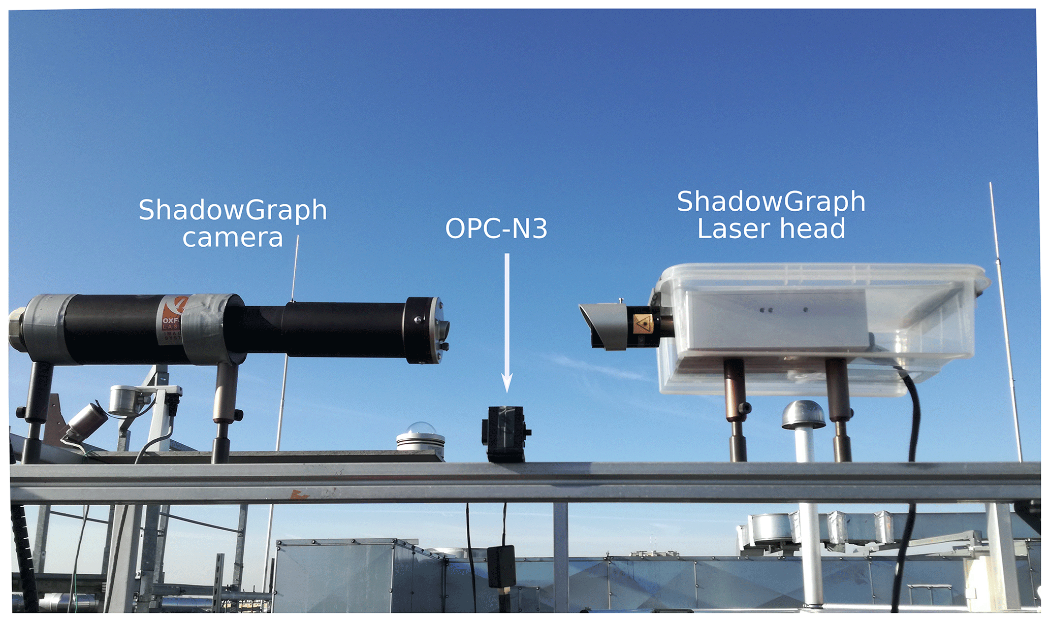
Figure 1 OPC-N3 and ShadowGraph at the Radiation Transfer Laboratory, Institute of Geophysics, Faculty of Physics, University of Warsaw, Poland.

2.1.1 VisiSize D30

The VisiSize D30 is a shadowgraph system manufactured by Oxford Lasers Ltd. The VisiSize D30 (hereafter called ShadowGraph) captures the shadow images of particles passing through a measurement volume between a laser head and a high-resolution camera. It can detect particles of different sizes and shapes in various suspensions in real time. The images are acquired by backlight illumination of a measurement volume using an infrared diode laser (808 nm). The camera is triggered in time with the laser pulses so that a single pulse of laser light occurs in each exposure of the camera. It can capture shadow images of particles with a maximum rate of 30 frames per second. The size and velocity of the captured particles are then measured by the ShadowGraph using software provided by the manufacturer based on the particle/droplet image analysis (PDIA) method. PDIA was first introduced by Kashdan et al. (2003, 2004) to measure industrial sprays. The system allows for retrieving microphysical properties such as shape, size, DSD(r), total droplet number concentration (N_c) and LWC.

Table 2 Technical specifications for the two instruments provided by the manufacturers, by Nowak et al. (2021) and Hagan and Kroll (2020).

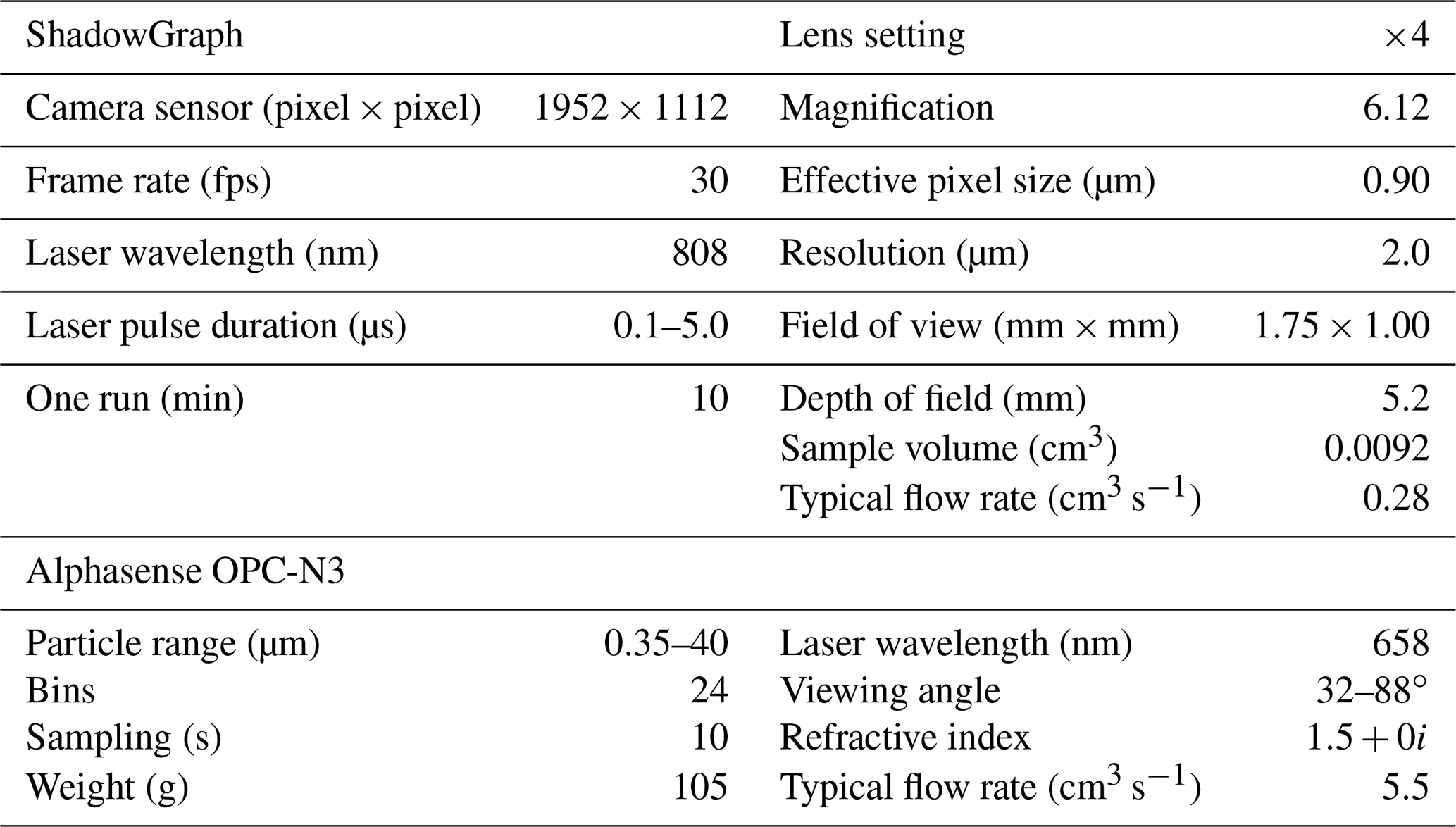
The ShadowGraph camera is equipped with different lens magnification settings, and this adjustment can change the resolution of the sample volume. The manufacturer provides calibration for three settings: ×1, ×2 and ×4. For this study, the magnification setting of ×4 was used, as it allows for measuring the smallest droplets. The effective pixel size for this magnification is 0.9 µm. The ShadowGraph collects data in runs; one run was set to last 10 min. There is a pause of around 1 s between runs to save the data. Table 2 presents more details on the ShadowGraph specifications. The ShadowGraph has already been used successfully to study cloud microphysics in both laboratory and in situ measurements. The droplet detection and sizing system of the ShadowGraph were described by Nowak et al. (2021) in detail. The data collected with ShadowGraph on orographic clouds, i.e. in fog conditions over the mountains, were analysed by Mohammadi et al. (2022).

2.1.2 OPC-N3

OPC-N3 is an optical particle counter developed by Alphasense Ltd. The device is constructed of a diode laser light (wavelength 658 nm) and an elliptical mirror that reflects the laser to a detector. The flow is perpendicular to the laser beam. By using a fan to force the flow, the device can operate continuously without the need to periodically replace the pump filters. OPC-N3 measures the particle number concentration (PNC) in 24 bins, in a diameter range of 0.35 to 40 µm. The PNC measured by the onboard algorithm is converted to PM₁, PM_2.5 and PM₁₀. OPC-N3 can measure the mass concentrations of particles up to 2000 µg m⁻³. The sensor returns information about the internal temperature and relative humidity. More information on the Alphasense OPC-N3 specification is provided in Table 2; more details about OPC-N3 can be found in Hagan and Kroll (2020).

3 Methods

3.1 Fog detection

To automatically retrieve data concerning fog events, calculations were performed to obtain the minimum concentration of droplets needed to create a fog. The Koschmieder formula (Eq. 1) relates visibility (VIS) to the extinction coefficient σ.

$$\begin{array}{}\text{(1)}& \mathrm{VIS}={\displaystyle \frac{\ln \mathrm{50}}{\mathit{\sigma }}}\end{array}$$

The extinction coefficient for spherical particles σ is defined by the following equation:

$$\begin{array}{}\text{(2)}& \mathit{\sigma }=\mathit{\pi }\int r^{\mathrm{2}}{Q}_{\mathrm{e}}\mathrm{DSD}\left(r\right)\mathrm{d}r,\end{array}$$

where r is the droplet radius, DSD(r) is the droplet size distribution and Q_e is the efficiency coefficient for extinction. To estimate the minimum N_c, it was assumed that fog consists of a monodisperse distribution of droplets with a radius of 9.76 µm (effective radius of droplets measured by ShadowGraph). From the Mie theory for the radius of 9.76 µm, the Q_e was calculated to be 2.17.

Based on Eqs. (1) and (2) the minimum concentration of droplets necessary to cause fog was 6.03 cm⁻³. For calculations of the microphysical properties of fog, data from ShadowGraph for which the droplet concentration is greater than or equal to 6.03 cm⁻³ were taken into account. During 5 d, 103 runs (each of 10 min) with detected fog were obtained.

3.2 ShadowGraph depth-of-field

When a droplet is at a distance from the camera's focal plane (i.e. a defocused droplet), the generated shadow image consists of a grey halo area around a dark interior circle. If the defocus distance increases, the halo area will grow faster than the total image area. It reaches a point where it takes over almost the whole particle image and eventually fades into the background. A criterion was set in the ShadowGraph software algorithm called focus rejection to avoid the sizing error that occurs in the above-mentioned situation. The particles with a halo area equal to or larger than 95 % of the total particle area are rejected based on this criterion.

To precisely calculate the sample volume in which the droplet can be detected, and subsequently the total droplet number concentration, an accurate measurement of the depth of field (DOF) is essential. The DOF, which is equal to the maximum defocus distance, is assumed by Kashdan et al. (2003) to be linearly dependent on the particle size for a diameter range between 18 and 145 µm.

However, Nowak et al. (2021) showed that for smaller droplets (e.g. cloud-size droplets), the focus rejection criterion plays a key role by imposing a significant constraint on the acceptable DOF. In such cases, the halo area around the droplet exceeds the focus rejection limit at a defocus distance shorter than the linearly size-dependent DOF assumed by Kashdan et al. (2003). Consequently, the relevant sample volume is affected by the focus rejection, which results in an underestimation of the total droplet number concentration.

Nowak et al. (2021) developed a correction method based on the focus rejection criterion in which the DOF for droplet diameter D_i is calculated as follows:

$$\begin{array}{}\text{(3)}& z_{\mathrm{95}|D_i}={\displaystyle \frac{\mathrm{0.95}}{(\mathrm{1}-\mathrm{0.95}{a}_{\mathrm{3}})(a_{\mathrm{1}}{D}_i+a_{\mathrm{2}})}}{\displaystyle \frac{\mathit{\pi }}{\mathrm{4}}}{\displaystyle \frac{(D_i+a_{\mathrm{4}}+a_{\mathrm{5}}{)}^{\mathrm{2}}}{{\mathrm{pix}}^{\mathrm{2}}}},\end{array}$$

where the constants a₁ and a₂ are calibration constants for a given lens magnification, while constants a₃, a₄ and a₅ refer to the halo blurring, pixelisation and diffraction. In addition, pix represents the effective pixel size equal to 0.9 µm for a ×4 lens magnification setting.

Subsequently, the sample volume for individual droplet i is calculated by multiplying the above DOF and ShadowGraph field of view (FOV) as follows:

$$\begin{array}{}\text{(4)}& V_i=\mathrm{2}{z}_{\mathrm{95}|D_i}(L_x-D_i)(L_y-D_i),\end{array}$$

where L_x and L_y are, respectively, the horizontal and vertical length of FOV (in µm). Eventually, to calculate the N_c, a sum over multiplicative inverse values of V_i must be divided by the total frame numbers F as shown below:

$$\begin{array}{}\text{(5)}& N_{\mathrm{c}}={\displaystyle \frac{\mathrm{1}}{F}}\sum _i{\displaystyle \frac{\mathrm{1}}{V_i}}.\end{array}$$

3.3 Uncertainty of the measurement

The data from ShadowGraph were integrated every 10 min. To calculate the uncertainty of the values (LWC, N_c, mean radius) calculated from ShadowGraph, it was assumed that the uncertainty is influenced by the effective pixel size of ShadowGraph of 0.9 µm and by the Poisson statistics. The formula for the DOF depends on the diameter of the droplet. The uncertainty of a given variable was calculated using the formula for the propagation of uncertainty.

Data from OPC-N3 were collected every 10 s, averaged every 10 min to compare with ShadowGraph. As the uncertainty of the OPC-N3 data, standard deviation was used, obtained by averaging the data over 10 min periods and the Poisson statistics.

3.4 Scope of compliance between OPC-N3 and ShadowGraph

ShadowGraph samples around 1000 cm³ of air over the period of 1 h. To obtain a smooth droplet size distribution spectrum from ShadowGraph, the data need to be averaged for a period longer than 10 min. The minimum averaging time needs to be chosen in such a way that the spectrum is smooth, and the time of averaging still allows for the analysis of spectrum changes over time. The data were averaged over 1 h¹. Figure 2a shows the volume droplet size distribution (vDSD(r)) and Fig. 2b the droplet size distribution (DSD(r)) of OPC-N3 and ShadowGraph. Formulas for DSD(r) and vDSD(r) are given, respectively, as

$$\begin{array}{}\text{(6)}& {\displaystyle }\mathrm{DSD}\left(r_{\mathrm{b}}\right)=N_{\mathrm{b}}\cdot {\left(V_{\mathrm{b}}\cdot \mathrm{\Delta }{r}_{\mathrm{b}}\right)}^{-\mathrm{1}},\text{(7)}& {\displaystyle }\mathrm{vDSD}\left(r_{\mathrm{b}}\right)=\mathrm{DSD}\left(r_{\mathrm{b}}\right)\cdot r_{\mathrm{b}}^{\mathrm{3}},\end{array}$$

where N_b is the number of droplets in a bin, V_b the volume of a bin, Δr_b the width of the bin and r_b the mean bin droplet radius.

Figure 2 The droplet size distribution DSD(r) ((b) and (d)) and volume droplet size distribution vDSD(r) ((a) and (c)) of OPC-N3 and ShadowGraph. The values obtained for each bin of OPC-N3 are shown in yellow, and ShadowGraph data, aggregated into the same bins as OPC-N3 are shown in blue. The data were averaged by 1 h (17 November 2021, 02:00:59–03:01:07 UTC). The right axis corresponds to OPC-N3. Panels (a) and (b) represent the bins from OPC-N3 as they are provided by the manufacturer. In panels (c) and (d), the last bin of OPC-N3 has been adjusted, and its range is (18.5–25.02] µm. In panel (c), the range of OPC-N3 bins taken into account for the calculations of LWC and N_c is shown in red and r_eff and mean radius in black. The number 1935 in panel (a) indicates the value of the last bin of OPC-N3.

Alphasense OPC-N3 manual specifies that OPC-N3 records droplet radiuses in the range of 0.175 to 20.000 µm. Fig. 2 shows that the last bin of OPC-N3 registers a much greater mass of droplets than it would appear from the distribution. This indicates that the last bin has not been properly assigned its right edge. In the last bin of OPC-N3 the particles of radiuses larger than 20.00 µm are also counted.

The last OPC-N3 bin contains a significant part of LWC; therefore it was not excluded from the analysis. However, a new mean radius for this bin was estimated based on ShadowGraph data. One histogram of DSD was created from all ShadowGraph data of fog events. The mean volume radius (r_V) was calculated for droplets bigger than 18.5 µm. The obtained r_V is 21.76 µm. Based on this calculation, the lower boundary of the OPC-N3 last bin is set as 18.5 µm, the mean radius is set to 21.76 µm and the upper boundary is set as 25.02 µm (the upper limit is set in such a way that the centre of the bin falls on the mean radius). Figure 2c shows the vDSD after adjustment of the last bin of OPC-N3.

Oxford Lasers states that the minimum value of the diameter that can be imaged by the ShadowGraph for a magnification of ×4 is 2 µm. The minimum diameter of fog droplets registered by ShadowGraph was 3.47 µm.

ShadowGraph spectrum has a peak in the bin of droplet mean radius of 2.925 µm. This peak is not visible in the OPC-N3 data. It appears to be a problem in recognising the actual size of small droplets by the algorithm. The pixel size of ShadowGraph is 0.9 µm, leading to a misinterpretation of droplets 2–3 pixels in size. In the article of Kashdan et al. (2003) there is a peak in the droplet distribution function for the bin with the smallest droplets. This is explained by the misclassification of small unfocused droplets. Identification of the droplets and their size is done by distinguishing the brightness between the shadow of the drop and the brightness of the background pixels. For fuzzy droplets, the difference is small, making it difficult to classify the droplets to the correct size. In our analysis, the droplets below a radius of 4 µm were excluded.

During the 5 d of the study, fog was observed for 17.2 h. Microphysical parameters such as N_c, LWC, r_eff and mean radius were calculated. For those calculations, droplets from the range of 4 to 25.024 µm were taken into account for both devices. In the case of OPC-N3, it corresponds to bins from 12 to 24. Bin 24 was taken into account as it contains a significant amount of LWC but after adjusting its mean radius to 21.76 µm. Droplets smaller than 4 µm were excluded from the comparison as ShadowGraph has problems correctly classifying them.

For the comparison of r_eff and mean radius, only the droplets from the range of 4 to 18.5 µm were taken into account for ShadowGraph and OPC-N3 (bins 12 to 23 of OPC-N3), as in this range, the registered sizes of droplets from both devices overlap without any adjustments. The droplet radius range, taken into account for each microphysics parameter, is shown in Appendix A Table A1.

Figure 2 shows that the values of DSD for OPC-N3 are smaller than for ShadowGraph. Appendix A presents a study regarding whether correcting the OPC-N3 data based on the refractive index (RI) allows for better data compliance with ShadowGraph.

Particles in OPC-N3 are assigned to the size bins based on the amount of light scattered. In Mie theory, the amount of light scattered can be linked to a specific size of a particle; to be able to use Mie theory, one needs to assume an appropriate RI of a particle. In OPC-N3, the manufacturer set the RI_OPC at 1.500+0.00i. The refractive index of pure water – RI${}_{\mathrm{water}}=\mathrm{1.331}+\mathrm{0.000}i$ (Hale and Querry, 1973) – is different from the one assumed in OPC-N3, which can lead to an incorrect assignment of the droplets to the correct bin based on their radius.

We analysed the effect of recalculating the assignment of droplets to specific bins using RI_water. As a result, we found out that the vDSD spectrum of OPC-N3 and ShadowGraph after RI correction does not overlap as well as when it was assumed RI_OPC; however, due to the greater representation of bigger droplets, a better comparison of LWC between the devices was obtained. In this study, the refractive index is the default OPC-N3 RI_OPC, and in the Appendix, the comparison to values calculated using RI_water is shown.

3.5 OPC-N3 temperature and relative humidity

Alphasense OPC-N3 reports temperature (T) and relative humidity (RH). The sensors are mounted inside the device. The registered values were compared with Vaisala WXT520, which is mounted on the roof of the Institute of Geophysics and measures ambient T and RH. As seen in Fig. 3a the T inside OPC-N3 is approximately 6 ^∘C higher than that of Vaisala WXT520. The circuit board system is most probably heating the inside of the device. This causes a drop in humidity within OPC-N3. When comparing the RH of OPC-N3 with Vaisala WXT520, it is seen that the RH within OPC-N3 is lower by around 20 %. The measurements presented were taken during the night and early morning. During the night, the value from OPC-N3 seems to be shifted by a constant value in comparison with Vaisala WXT520. The temperature and RH registered by OPC-N3 rapidly change after sunrise (06:00 UTC). The OPC-N3 is made of black plastic, which is probably heated by sunlight; the higher temperature of the body affects the inside humidity. This leads to the conclusion that the T and RH reported by OPC-N3 cannot be used as the values of ambient conditions and cannot be easily corrected. Furthermore, a higher T and lower RH within OPC-N3 may impact on the droplet size due to the evaporation process.

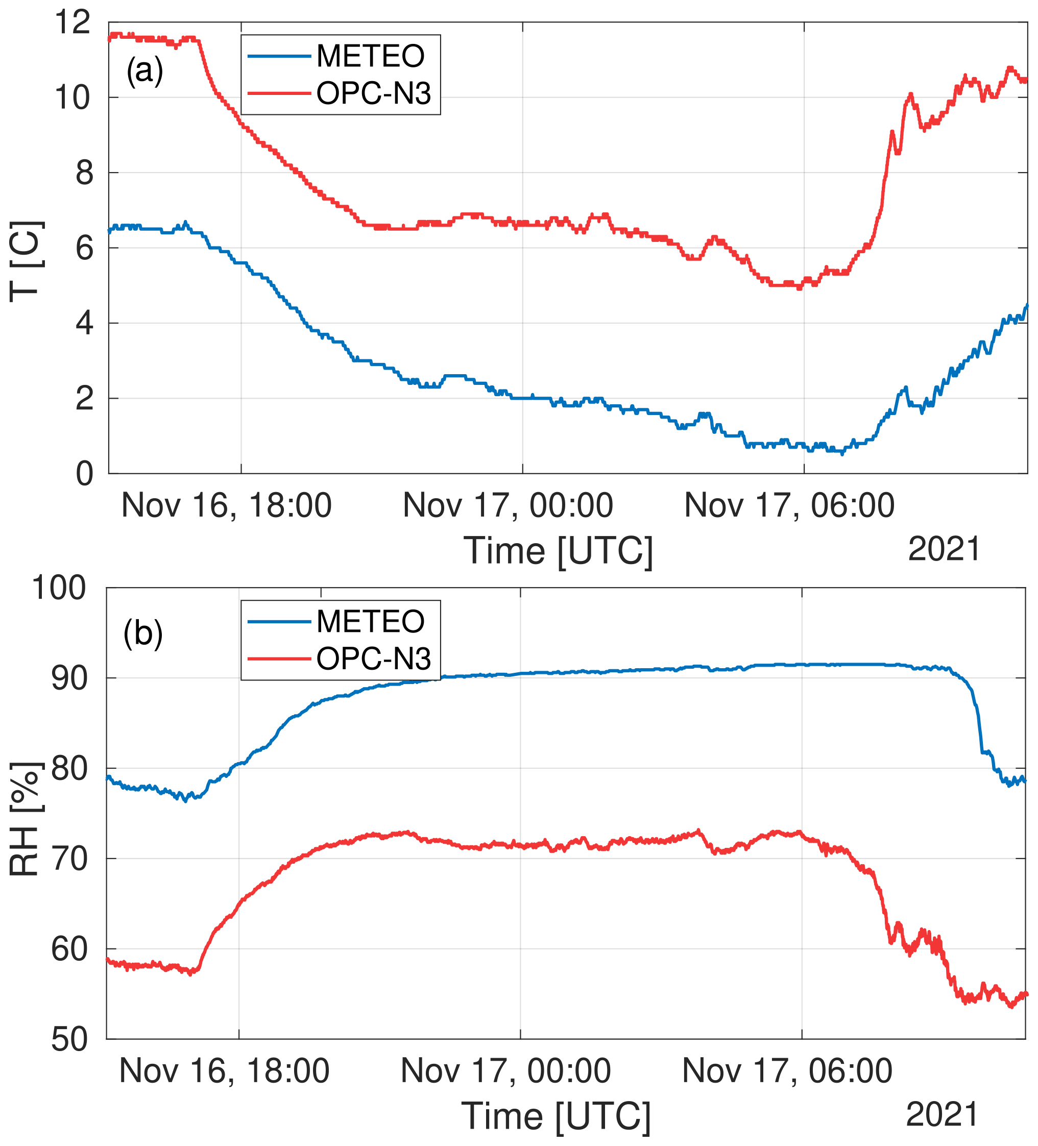
Figure 3 Comparison between OPC-N3 (red line) with Vaisala WXT520 (blue line) of (a) temperature (T) and (b) relative humidity (RH). Devices mounted on the roof of the Institute of Geophysics, with sunrise at 06:00 UTC.

4 Results

4.1 Microphysical properties of fog

The data obtained from all the dates of fog occurrence (listed in Table 1) were used for comparison of microphysical properties of fog between OPC-N3 and ShadowGraph.

4.1.1 Liquid water content

LWC results are shown in Fig. 4a. The LWC calculated from ShadowGraph ranges from 0 to 0.2 g m⁻³. The comparison between OPC-N3 and ShadowGraph shows a linear relationship between devices. The OPC-N3 values are almost 2 times lower than those from ShadowGraph. The Pearson correlation coefficient (PCC) is 0.92.

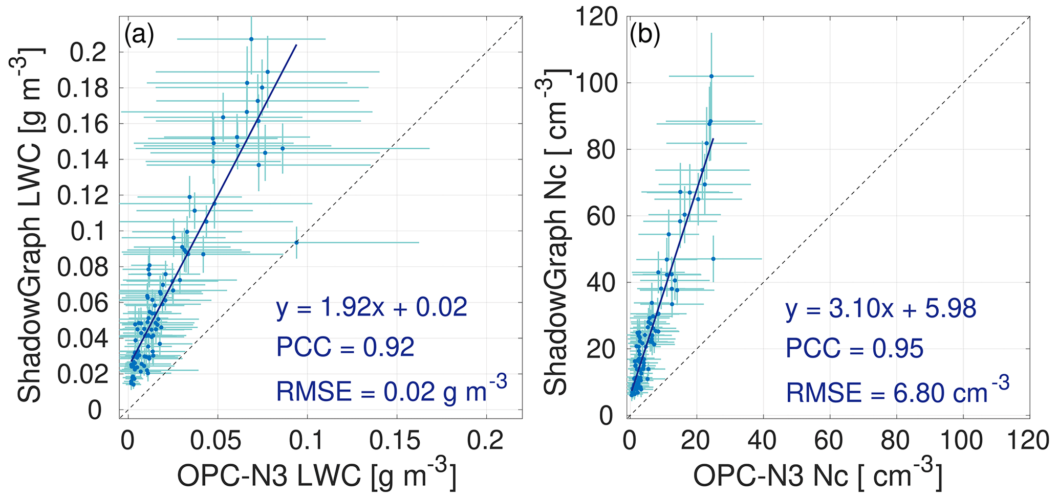
Figure 4 Comparison between ShadowGraph and OPC-N3 of (a) liquid water content (LWC) and (b) total droplet number concentration (N_c). Each point represents a value measured over a 10 min period. Blue points represent data retrieved from the devices, solid deep blue lines represent the linear fit to the data and bars represent the estimation of uncertainty.

Values such as LWC, N_c and droplet diameter statistics obtained from OPC-N3 can be corrected using a linear regression curve of the form $y=ax+b$, where x is the measured value from OPC-N3, a and b are calculated coefficients, and y is the measured value from ShadowGraph. The linear regression coefficients, PCC and RMSE, for LWC are presented in Appendix B Table B1.

4.1.2 Total number concentration

The droplet number concentration is shown in Fig. 4b; the values span from below 10 to around 100 cm⁻³ for ShadowGraph. There is a high Pearson correlation coefficient equal to 0.95 for the comparison with OPC-N3. The values obtained from OPC-N3 are lower than those obtained from ShadowGraph. The linear regression coefficients, PCC and RMSE, for N_c are presented in Appendix B Table B1.

4.1.3 Droplet diameter

Four different droplet diameter statistical moments were calculated: the arithmetic mean r, the surface mean r_S, the volume mean r_V and the effective radius r_eff. The values were calculated using a formula for statistical moments. To calculate r_eff, the following formula was used:

$$\begin{array}{}\text{(8)}& r_{\mathrm{eff}}=\left(\sum _{i=\mathrm{1}}^m{r}_i^{\mathrm{3}}\cdot N_i\right)\cdot {\left(\sum _{i=\mathrm{1}}^m{r}_i^{\mathrm{2}}\cdot N_i\right)}^{-\mathrm{1}},\end{array}$$

where N_i in the case of OPC-N3 is the concentration of droplets in the volume of the bin, and m denotes the number of bins. For ShadowGraph, m denotes the number of droplets and $N_i=(F{V}_i{)}^{-\mathrm{1}}$, where V_i is the volume in which the droplets were measured. To calculate the mean radius r, the following formula was used:

$$\begin{array}{}\text{(9)}& r=\left(\sum _{i=\mathrm{1}}^m{r}_i\cdot N_i\right)\cdot {\left(\sum _{i=\mathrm{1}}^m{N}_i\right)}^{-\mathrm{1}}.\end{array}$$

To calculate the mean surface radius r_S, the following formula was used:

$$\begin{array}{}\text{(10)}& r_{\mathrm{S}}={\left(\left(\sum _{i=\mathrm{1}}^m{r}_i^{\mathrm{2}}\cdot N_i\right)\cdot {\left(\sum _{i=\mathrm{1}}^m{N}_i\right)}^{-\mathrm{1}}\right)}^{\mathrm{1}/\mathrm{2}}.\end{array}$$

To calculate the mean volume radius r_V, the following formula was used:

$$\begin{array}{}\text{(11)}& r_{\mathrm{V}}={\left(\left(\sum _{i=\mathrm{1}}^m{r}_i^{\mathrm{3}}\cdot N_i\right)\cdot {\left(\sum _{i=\mathrm{1}}^m{N}_i\right)}^{-\mathrm{1}}\right)}^{\mathrm{1}/\mathrm{3}}.\end{array}$$

Figure 5 shows the r_eff and Fig. 6a the mean radius, Fig. 6b the mean surface radius and Fig. 6c the mean volume radius. The r_eff is between 8.05 and 11.71 µm for ShadowGraph. There is a modest correlation coefficient between the devices for all mean radiuses. The linear regression coefficients, PCC and RMSE, are presented in Appendix B Table B1.

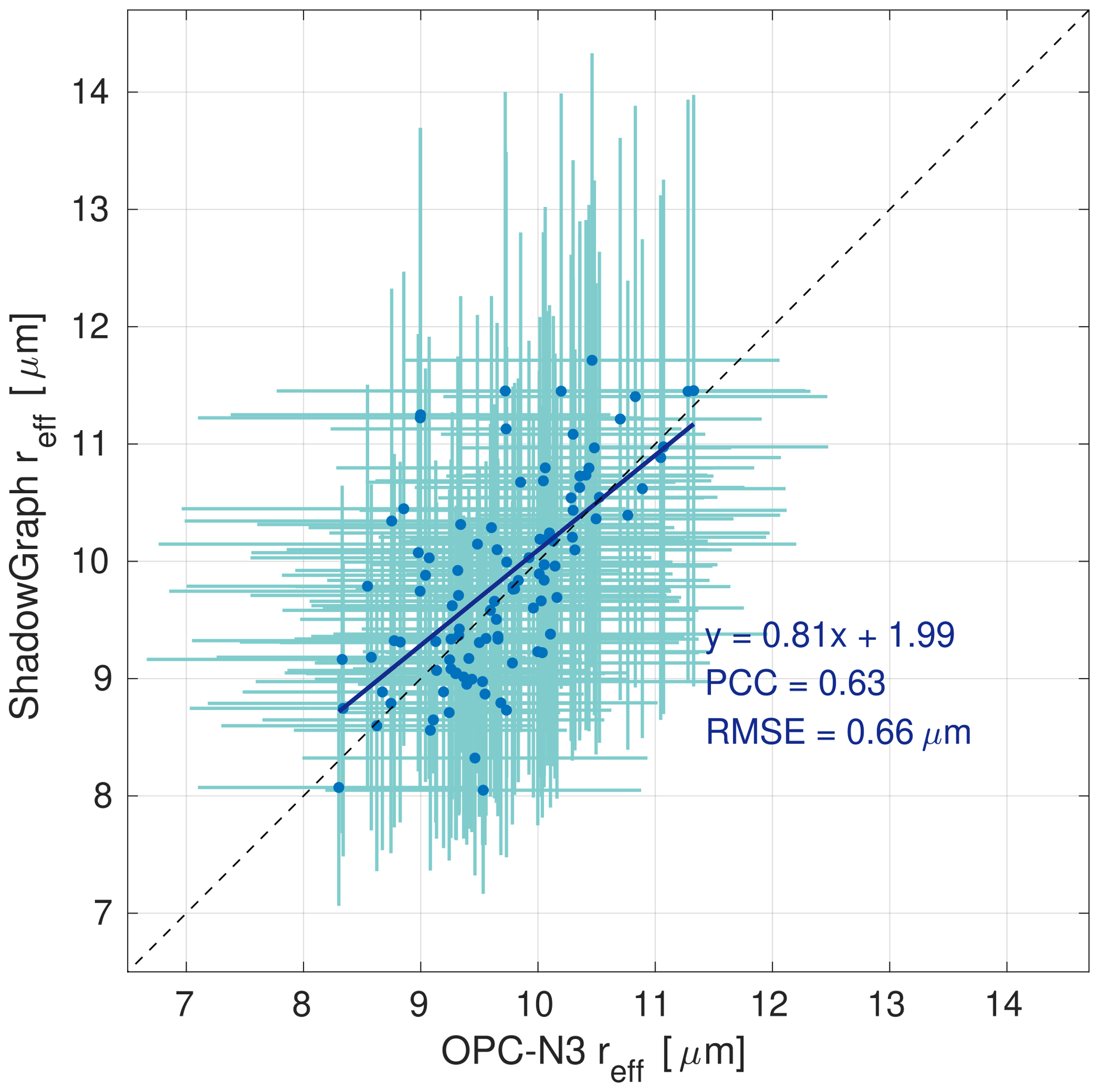
Figure 5 Comparison between ShadowGraph and OPC-N3 of r_eff (µm). Each point represents a value averaged over 10 min, and the bars represent the estimation of uncertainty. Blue points and lines represent data retrieved from the devices, and solid deep blue lines represent the linear fit to the data.

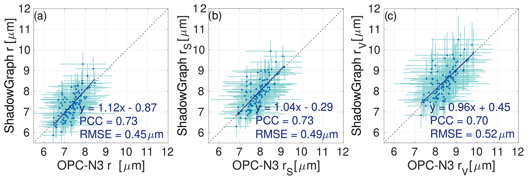
Figure 6 Comparison between ShadowGraph and OPC-N3 for (a) mean radius (µm), (b) mean surface radius (µm) and (c) mean volume radius (µm). Each point represents a value averaged over 10 min, and the bars represent the estimation of uncertainty. Blue points and lines represent data retrieved from the devices, and solid deep blue lines represent the linear fit to the data.

5 Case study

During the measurements, five fog events were registered. Most of them lasted less than 2.5 h. The longest event occurred at night from 16 to 17 November 2021. As this case of fog lasted for almost 8 h, it was chosen for the case study in this section.

5.1 Overview of weather conditions

On 16 November 2021, Poland was in the saddle region, between two highs over the North Atlantic and Ukraine. The anticyclone above Ukraine moved towards the Caspian Sea, causing the pressure to drop from 1008 hPa at 18:00 UTC to 1004 hPa around 07:00 UTC on 17 November 2021. Atmospheric conditions at the saddle point resulted in a decrease in wind speed during the measurements. The wind blowing from the direction of 150^∘ was on average 2.2 m s⁻¹, which favoured the formation of fog.

Fog started to form around 21:15 UTC. The sky was clear before fog occurrence (infrared incoming surface flux was around 250 W m² before 20:00 UTC). The infrared flux started to rise around 21:00 UTC and dropped around 22:16 UTC, suggesting a temporary disappearance of fog. At approximately 04:00 UTC, the infrared flux started to decrease, and after sunrise, the total flux increased – the line representing the total flux is jagged, which suggests that in the said morning, there was a layer of thin clouds above the fog.

From 18:00 UTC, on 16 November 2021, the air temperature decreased from 5.4 ^∘C to a minimum of 0.5 ^∘C just before 07:00 UTC the next day. The temperature then started to increase, and the process of fog dissipation started. Appendix C Fig. C1 shows the atmospheric situation on the measurement site in detail, and Appendix C Fig. C2 presents the radiosounding from 00:00 UTC 17 November 2021 from Legionowo, which is near the city of Warsaw.

In Appendix C, Fig. C1a shows the scattering coefficient at 525 nm measured by an Aurora 4000 nephelometer at dry conditions (the humidity inside Aurora 4000 during the measurements was below 30 %). The values increased from 178 Mm⁻¹ at 18:00 UTC to 250 at 19:30 UTC and then oscillated between 250–260 Mm⁻¹ until 23:15 UTC, and then they continuously decreased to 170 Mm⁻¹ at 07:00 UTC. Values above 200 Mm⁻¹ suggest moderate smog conditions. The increase in the scattering coefficient after 18:00 UTC was probably due to air pollution caused by the activation of the house heating system and traffic emissions.

The PM values obtained from OPC-N3 are presented in Fig. 7. The PM₁ was around 17 µg m⁻³ at 18:00 UTC and increased to 125 µg m⁻³ at 23:00 UTC, then the PM₁ value decreased. PM₁₀ data exhibit a different behaviour from PM1. Between 21:00 and 22:30, 22:45 and 04:00, and 04:20 and 06:10 UTC, episodes of significant increase and decay in PM₁₀ value were observed. For each episode, PM₁₀ reached, respectively, 14 960, 12 550 and 6897 µg m⁻³. A similar pattern was observed in PM_2.5 but less pronounced (1354, 1148 and 893 µg m⁻³). Such values are unrealistic for the city of Warsaw; the values are biased due to high humidity and fog droplet contamination. These episodes correspond to three periods of fog events. In Fig. 7b, the estimated values of LWC are presented for OPC-N3 and ShadowGraph.

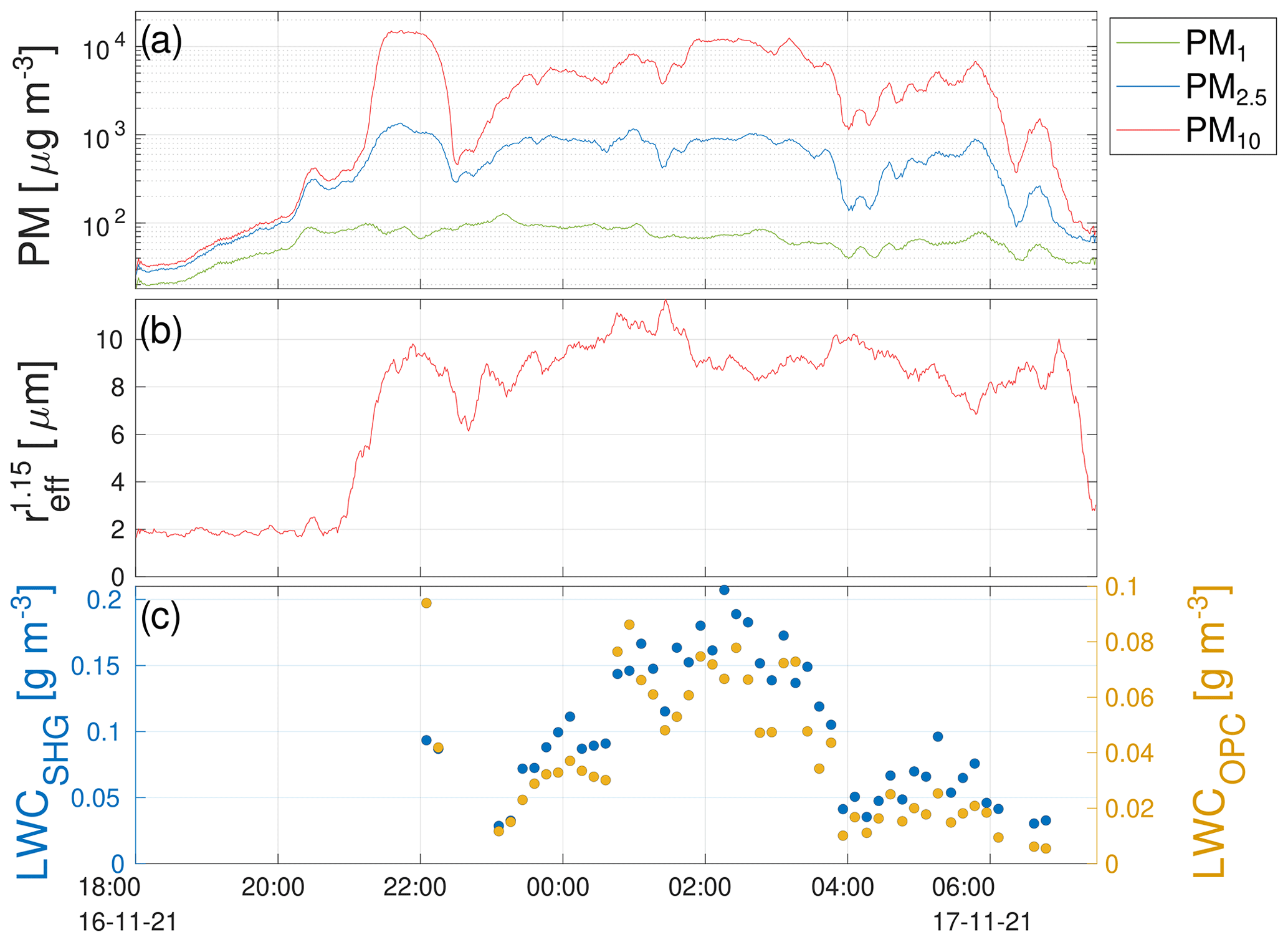
Figure 7 Situation during the night of 16 November 2021: (a) PM₁, PM_2.5 and PM₁₀ obtained from Alphasense OPC-N3. The data from this instrument were collected every 10 s, and later a running mean over a 10 min window was applied to smooth the data. (b) Effective radius calculated from OPC-N3 for droplets (radiuses from 1.15 µm were taken into account). (c) LWC obtained from ShadowGraph and OPC-N3. The values were calculated every 10 min. LWC was calculated only for fog occurrence (automatic fog detection was described in Sect. 3.1).

The data collected from OPC-N3 allow the effective radius to be calculated. Fig. 7b shows the effective radius calculated from the droplets that have a radius bigger than 1.15 µm ($r_{\mathrm{eff}}^{\mathrm{1.15}}$). The $r_{\mathrm{eff}}^{\mathrm{1.15}}$ rapidly increases after the fog onset. When there are high concentrations of PM, based on $r_{\mathrm{eff}}^{\mathrm{1.15}}$, it is possible to distinguish an episode of haze from an episode of fog.

5.2 Evolution of the droplet spectrum

In this subsection, the evolution of the droplet spectrum is shown for the period between 22:00 UTC on 16 November and 07:00 UTC on 17 November. Figure 8 shows the vDSD(r) for OPC-N3 and ShadowGraph. In one plot, the data for the average of 1 h are shown.

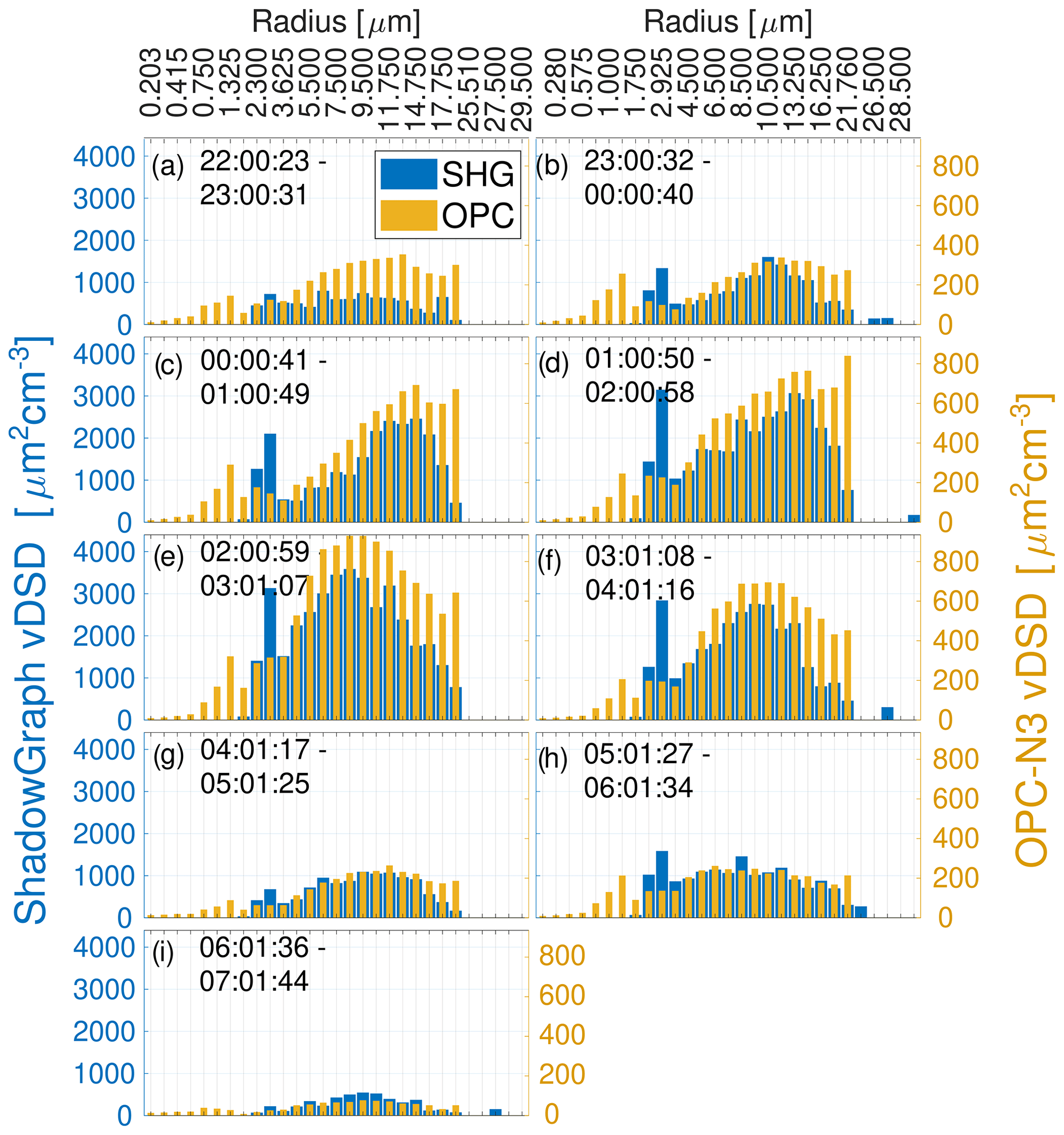
Figure 8 Volume droplet size distribution (vDSD(r)). Data obtained from ShadowGraph are shown in blue and from OPC-N3 in yellow. Panels from (a) to (i) represent consecutive hours between 22:00 UTC on 16 November and 07:00 UTC on 17 November.

Figure 8 shows a relatively good agreement between devices on the behaviour of the droplet spectrum. During the night of 16 November, the first fog event occurred from 21:00 to 22:20 UTC. Due to some connection errors, the ShadowGraph was set at 22:00 UTC. Moreover, during the first 10 min run, it did not recognise all the droplets that passed through it, probably due to the steamed lens.

The spectrum obtained from OPC-N3 consists of a two-mode distribution. The first mode has a maximum for bin mean radius 1.33 µm, and its location remains steady at night. The second-mode peak during hours 23:00–02:00 UTC moves from 11.75 to 14.75 µm. During this time, the fog evolved, and the value of the vDSD(r) increased. The maximum intensity of the fog was observed at 02:00–03:00 UTC, and the peak of the second mode rapidly changed to 8.50 µm. After 03:00 UTC, the second mode of droplet distribution flattened out, and the fog started to disappear. The data obtained from ShadowGraph followed the same pattern and the values obtained from ShadowGraph were greater. From 02:00 to 03:00 UTC, the maximum value of the vDSD(r) was 930 µm² cm⁻³ for OPC-N3 and 3586 µm² cm⁻³ for ShadowGraph.

6 Conclusions

The low-cost Alphasense OPC-N3 optical particle counter was tested for its application in the measurement of fog droplets and compared to Oxford Lasers VisiSize D30 ShadowGraph. The following results are obtained from the current work.

• In this article, we have shown that OPC-N3 registers fog droplets. Badura et al. (2018) showed that the previous version of Alphasense OPC overestimates PM values in high humidity. Our results are in line with this article; OPC-N3 in the case of high humidity (RH = 80 %–90 %) can overestimate PM values. During this study, the value of PM₁₀ reached above 15 mg m⁻³. Such high values cannot be explained only by the hygroscopic growth of aerosols. The high PM values are associated with fog occurrence and are a result of the count of fog droplets by OPC-N3. The main point of this article was to verify the hypothesis that the values are overestimated because OPC-N3 counts fog droplets.

• OPC-N3 can be used to automatically detect the fog. After fog onset, the effective radius for particles bigger than aerosol (only droplets from bins 7 and higher taken into account) drastically increases (from a value of 2 to around 6–10 µm) and stays high for the duration of the fog.

• The manual of OPC-N3 provides information that OPC-N3 counts droplets diameters up to 20 µm. However in this study we observed that the last bin (diameter 18.5–20 µm) of OPC-N3 counts not only drops to 20 µm but also larger. Because this instrument is mainly used for aerosol measurements, which are usually not present at this size, this problem has not been described before. This fact was possible to observe by presenting the results from ShadowGraph and OPC-N3 as the volume droplet size distribution vDSD(r). We estimated based on ShadowGraph data that the last bin of OPC-N3 for this analysis collects droplets from 18.5–25.02 µm.

• The minimal practical radius that can be measured by ShadowGraph is approximately 3.5–4 µm for lens magnification ×4. The manual provided by Oxford Lasers reports that the minimum radius resolution of ShadowGraph is 1.01 µm. However, during the measurements, ShadowGraph did not record droplets smaller than 1.73 µm. Interestingly, the results reveal that there were non-physical concentrations of droplets in bin (2.6–3.24 µm). As we stated in Sect. 3.4, this peak probably comes from noise and problems with the wrong diameter assignment of small defocused droplets. As there were some limitations in comparing the radius ranges of both devices, the range of radius taken for comparison in this article was from 4 µm to 18.5 or 25.02 µm.

• The LWC, N_c, r_eff and the statistical moments of radius were calculated based on the data obtained from OPC-N3. The values were compared with those retrieved from ShadowGraph. Overall, these results suggest that there is a high correlation between OPC-N3 and ShadowGraph. OPC-N3 can be used to measure fog microphysics; however, the values reported by OPC-N3 need to be corrected.

• We have shown that the measured T and RH by OPC-N3 are biased. As shown in Sect. 3.5 OPC-N3 T is higher by 6 ^∘C, and RH is lower by 20 % compared to ambient T and RH. After sunrise, those values change, probably because of device case heating by solar radiation, and because of this, it is not possible to propose a correction of the measured T and RH by OPC-N3.

• The OPC-N3 lowers the values compared to ShadowGraph; in the case of LWC, the values are 1.92 times lower and in the case of N_c 3.10 times lower. As OPC-N3 uses a default RI for radius calculations, it was investigated whether applying the correction of the RI would improve the compatibility of the instruments (this issue is addressed in Appendix A). After correction, an improvement in LWC was observed; OPC-N3 data were 0.88 times smaller than the ShadowGraph values. However, applying the RI correction caused a shifting of the assigned radius of droplets registered by OPC-N3 to higher values. This resulted in a better compliance between OPC-N3 and Shadowgraph in LWC; however it decreased compliance in the effective radius. Applying RI correction does not appear to improve the consistency of the results. It might be that Alphasense has a built-in processing of the data while assigning it to the bin size. The underestimated results from OPC-N3 appear to be due to the fact that OPC-N3 counts fewer droplets than the ShadowGraph and not from their wrong assignment to the correct bin size. The reason for fewer droplets may be their evaporation due to the fact that the inside of the OPC-N3 has a higher temperature and lower humidity than environmental values. The second possibility could be that the open path inside of OPC-N3 allows the flow to expand, and this changes the droplet number concentration. The third reason could be that when the fan speed, which drives the flow inside the OPC-N3, changes, the algorithm does not properly adjust the amount of sampled air.

OPC-N3, due to its dimensions and low weight, can be mounted on UAVs, cable cars or balloons. Such works have been performed with small OPCs by Posyniak et al. (2021), Habeck et al. (2022) and Girdwood et al. (2020). The main objective of that research was to investigate changes in PM in the vertical profile. Our work presents a new applicability of OPC-N3 within UAVs (unmanned aerial vehicles) to measure the vertical profiles of the microphysical properties of fog. Another application of our study could be to produce inexpensive fog detection systems in airports or automatic fog monitoring systems on roads. Taking the effective radius of droplets received from OPC-N3 into consideration, it is possible to differentiate the low-visibility situations between fog conditions (which are not hazardous for people) from haze events, when highly polluted air can cause health risks to people.

Appendix A

A1 Correction of OPC-N3 due to refractive index

Optical particulate matter devices operate by measuring the light scattered by a particle. The Mie theory allows one to relate the amount of light scattered by a particle to its size, assuming particle sphericity. OPC-N3 has an elliptical mirror that sums up the amount of light scattered between angles 32–88^∘ (Hagan and Kroll, 2020).

The proposed correction of the refractive index changes the bin edges of OPC-N3. First, the theoretical scattering cross section (C_scat) was calculated for two RIs, one assumed in the OPC-N3 and one for water. The theoretical values of Mie scattering were calculated for 6000 points of logarithmic spaced radiuses. The curve was then smoothed by running the mean function (the mean was taken over 100 points). Later, for each mean radius of an OPC-N3 bin (r_old), C_scat was found on the calibration curve derived for RI_OPC (brown line with red dots in Fig. A1). Then the obtained C_scat values were transferred on the curve for RI_water (deep blue line) and their corresponding radius (r_new) (blue points in Fig. A1). In the following figures, the microphysical properties were calculated for the uncorrected radiuses r_old and the corrected ones r_new.

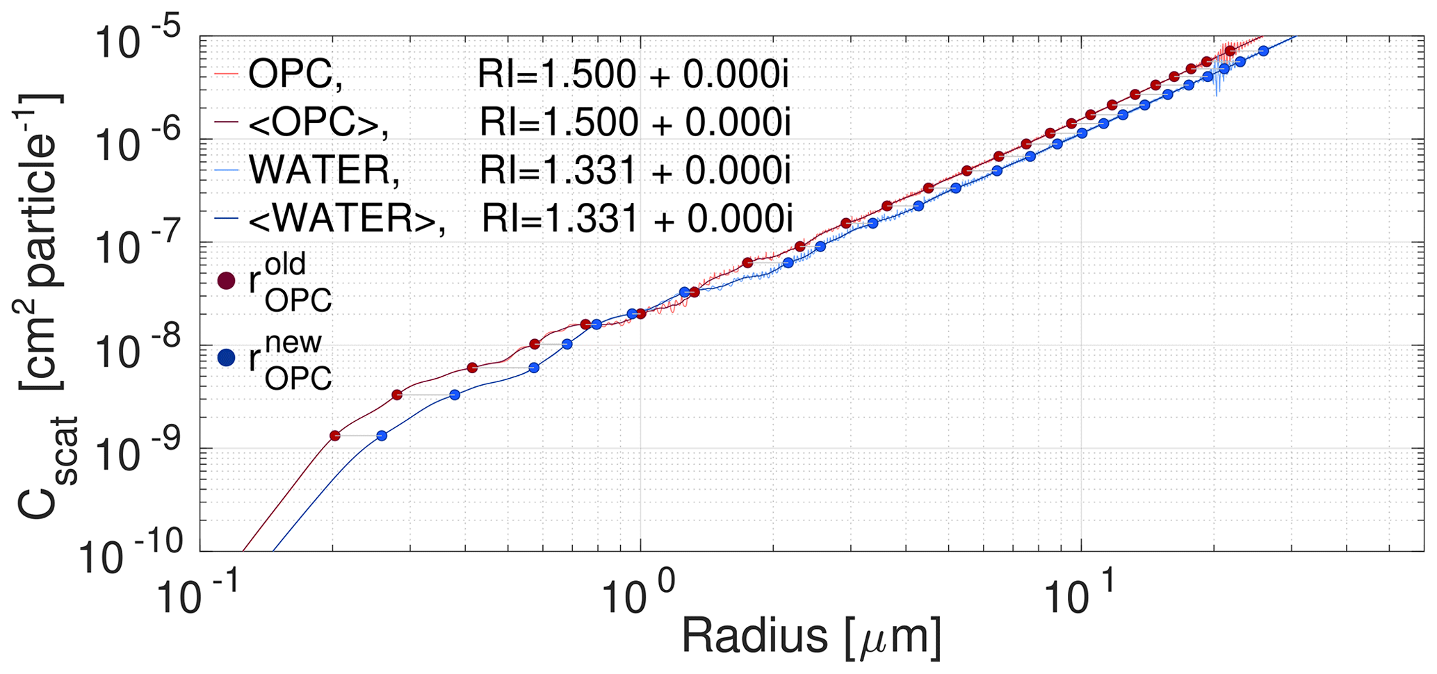
Figure A1 Theoretical scattering cross section C_scat calculated by the Mie theory for refractive index assumed by Alphasense in OPC-N3 (1.500+0.00i) and RI for pure water (1.331+0.000i) integrated for scattering angles 32–88^∘. Curves were smoothed by running mean (lines denoted as <OPC> and <WATER>). Points indicate the C_scat values at each middle radius of the bin (red dots) and blue dots the corrected radius values assuming the RI of water.

In the main text, droplets with radiuses from 4 to 18.5 µm (for r_eff, r, r_S, r_V) or 25.02 µm (for LWC, N_c) were taken into account. In this section, we show figures that compare the data not corrected (RI_OPC, represented in blue) to the data after the RI correction (RI_water, depicted in red). In the case of RI_water, the bin edges of OPC-N3 were shifted. The 18.5 µm edge was shifted to 22.03, and 25.02 µm was shifted to 28.31 µm. In the case of RI_water, the range of droplet radius taken into account for comparison between OPC-N3 and ShadowGraph was from 3.82 to 23.51 µm (for r_eff, r, r_S, r_V or 28.31 µm (for LWC, N_c); the appropriate ranges are listed in Table A1.

Table A1 The range of droplet radius which was taken into account for the calculation of microphysical properties of fog.

A2 Microphysical properties of fog

LWC results are shown in Fig. A2a. Applying the RI correction reduces the difference in LWC between devices; OPC-N3 shows values 0.88 smaller than those from ShadowGraph. The droplet number concentration is shown in Fig. A2b; the proposed RI correction does not make a significant improvement in the N_c data. In the case of LWC and N_c, PCC and RMSE are similar regardless of whether the correction was applied or not. The linear regression coefficients, PCC and RMSE, for LWC are presented in Appendix B Table B1.

Figure A2 Comparison between ShadowGraph and OPC-N3 of (a) liquid water content (LWC) and (b) total droplet number concentration (N_c). Each point represents a value measured over 10 min. Solid blue and red lines represent the linear fit to the data. Blue points and lines represent data retrieved from the devices, and red points and lines represent data after correction of the refractive index for OPC-N3.

The r_eff is shown in Fig. A3. The RI correction is only applied to OPC-N3; however, the RI correction affects the bin boundaries, which also has an impact on the data from ShadowGraph (the droplet radius range taken into account is wider after RI correction).

Applying the RI correction caused the shifting of the assigned radiuses of droplets registered by OPC-N3 compared to ShadowGraph (Fig. A3). The RMSE is higher between OPC and ShadowGraph than without correction. As the droplets are assumed to be larger, the LWC obtained is higher.

Figure A4 shows the evolution of the vDSD during D-16.11 fog case. The vDSD obtained from OPC-N3 is less consistent with the vDSD obtained from ShadowGraph than it was in the case without RI correction. The OPC-N3 vDSD consists of two modes, one with a peak around 0.8 µm and other around 14 µm. The second mode is shifted towards bigger droplet diameters compared to the distribution from ShadowGraph. Applying such a correction does not appear to improve the consistency of the results. It might be that Alphasense has a built-in processing of the data while assigning the bin size. The underestimated results from OPC-N3 appear to be due to the fact that OPC-N3 counts fewer droplets than the ShadowGraph and not from their wrong assignment to the correct bin size.

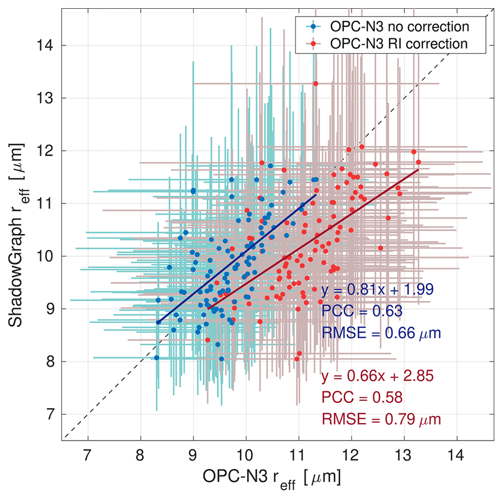
Figure A3 Comparison between ShadowGraph and OPC-N3 of $<r_{\mathrm{eff}}>$ (µm). Each point represents values averaged over 10 min, and the bars represent the estimation of uncertainty. Solid blue and red lines represent the linear fit to the data. Blue points and lines represent data retrieved from the devices, and red points and lines represent data after correction of the refractive index for OPC-N3.

Figure A4 Volume droplet size distribution (vDSD(r)) after applying RI correction to the data from OPC-N3. The bin mean radiuses are different in comparison to Fig. 8. The data obtained from ShadowGraph are shown in blue and from OPC-N3 in yellow. Panels from (a) to (i) represent consecutive hours between 22:00 UTC on 16 November and 07:00 UTC on 17 November. The bin value which is out of range has an assigned numerical value.

Appendix B

Table B1 The linear regression coefficients, Pearson's correlation coefficient (PCC) and the root mean square error (RMSE) for LWC, N_c, r_eff, r, r_S and r_V. The linear regression was obtained for data without RI correction and with RI correction applied. The linear regression curve of the form $y=ax+b$ was fitted to the respective quantity, where x is the measured value from OPC-N3, a and b are calculated coefficients, and y is the measured value from ShadowGraph.

Appendix C

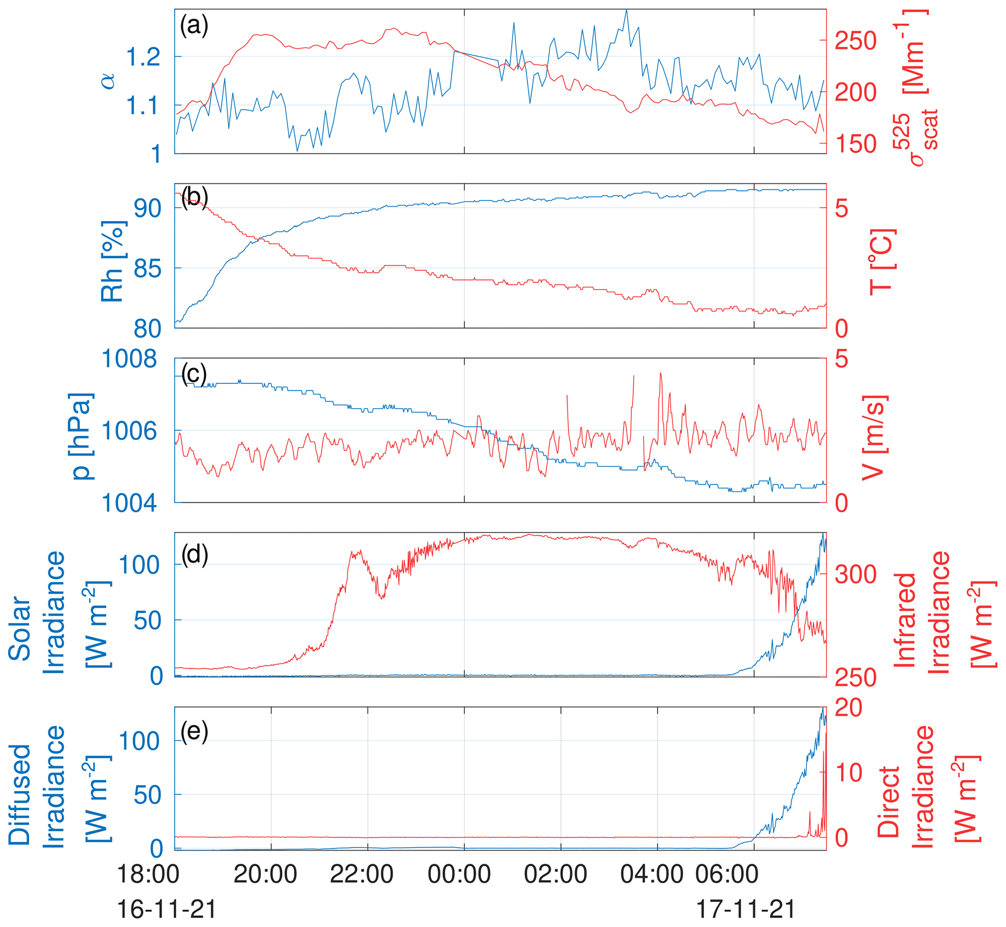
Figure C1 Situation during the night of 16 November 2021: (a) scattering coefficient $\left({\mathit{\sigma }}_{\mathrm{scat}}^{\mathrm{525}}\right)$ and Ångström exponent obtained from Ecotech Aurora 4000. The data from this instrument were collected every 5 min. (b) Temperature (T) and relative humidity (RH) obtained from Vaisala WXT520. The data from this instrument were collected every minute. (c) Local pressure (p) and mean wind velocity (V) obtained from Vaisala WXT520. (d) Total and infrared irradiance and (e) diffused and direct irradiance. The data came from apparatus mounted in the Radiation Transfer Laboratory, Faculty of Physics, University of Warsaw, Poland.

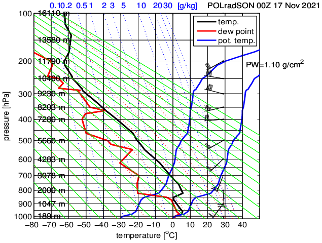
Figure C2 Radio sounding from 00:00 UTC 17 November 2021 from Legionowo (near Warsaw), Poland.