SAGE III/ISS aerosol/cloud categorization and its impact on GloSSAC

The Stratospheric Aerosol and Gas Experiment on the International Space Station (SAGE III/ISS) began its mission in June 2017. SAGE III/ISS is an updated version of the SAGE III on Meteor (SAGE III/M3M) instrument and makes observations of the stratospheric aerosol extinction coefficient at wavelengths that range from 385 to 1550 nm with a near-global coverage between 60^∘ S and 60^∘ N. While SAGE III/ISS makes reliable and robust solar occultation measurements in the stratosphere, similar to its predecessors, interpreting aerosol extinction measurements in the vicinity of the tropopause and in the troposphere has been a challenge for all SAGE instruments because of the potential for cloud interference. Herein, we discuss some of the challenges associated with discriminating between aerosols and clouds within the extinction measurements and describe the methods implemented to categorize clouds and aerosols using available SAGE III/ISS aerosol measurements. This cloud/aerosol categorization method is based on the results of Thomason and Vernier (2013), with some modifications that now incorporate the influence of recent volcanic/pyrocumulonimbus (PyroCb) events. Herein we describe this new cloud/aerosol categorization algorithm, demonstrate how it identifies enhanced aerosols and aerosol–cloud mixture in the lower stratospheric region, and discuss the impact of this cloud-filtering algorithm on the latest release of the Global Space-based Stratospheric Aerosol Climatology (GloSSAC) data set.

1 Introduction

The importance of stratospheric aerosol in determining the energy balance of the atmosphere has been well documented (e.g., Hofmann and Solomon, 1989; Fahey et al., 1993; Minnis et al., 1993; Kloss et al., 2021; Sellitto et al., 2022a, b). Recent years have witnessed frequent small to moderate volcanic eruptions as well as wildfire/pyrocumulonimbus (PyroCb) events that injected aerosols into the stratosphere, which resulted in radiative, chemical, and dynamical impact (Peterson et al., 2018; Yu et al., 2019; Kablick et al., 2020; Knepp et al., 2022; Sellitto et al., 2022b). Additionally, studies have shown that relatively smaller aerosol perturbations can also have radiative impact in the stratosphere (Vernier et al., 2011). Therefore, having accurate information of stratospheric aerosol extinction during and following such events and having the ability to distinguish between aerosols associated with these events and clouds is highly important. The objective of this study is to develop an aerosol–cloud separation algorithm that enables this distinction under perturbed conditions following events such as volcanic eruptions and PyroCb events.

Previous cloud/aerosol discrimination studies (e.g., Kent and McCormick, 1991; Kent et al., 1993; Wang et al., 1994; Kent et al., 1997a, b; Thomason and Vernier, 2013) relied on the use of multi-wavelength SAGE extinction coefficient measurements to infer information about particle size. Kent et al. (1993) developed a method to separate aerosol and clouds using an extinction coefficient distribution based on SAGE II measurements at 525 and 1020 nm. A key finding of Kent et al. (1993) was that optically thin clouds are aerosol–cloud mixtures, and they concluded that the transition from aerosol to aerosol/cloud occurs over a continuum. Wang et al. (1994) later investigated aerosol–cloud interaction of tropical high clouds using the same wavelength combination as Kent et al. (1993), but with additional information of temperature to identify the presence of high clouds in the tropical region. A different approach using three wavelength combinations (525, 1020, and 1550 nm) was later developed by Kent et al. (1997a) for SAGE III/M3M to identify cloud height.

Herein, we describe a cloud-screening algorithm for SAGE III/ISS to study the challenges in identifying pure aerosol and aerosol–cloud mixture from SAGE III/ISS observations and their impact on the development of the latest version of the Global Space-based Stratospheric Aerosol Climatology (GloSSAC v2.2). It is worthwhile to note here that the aerosol record post-2017 witnessed several volcanic eruptions and wildfire events that injected particles into the stratosphere, further complicating the separation of aerosol and clouds near the tropopause. Thomason and Vernier (2013) (hereafter TV13) used SAGE II observations from a volcanically quiescent period (1999–2005) to study the challenges in separating aerosol and cloud within the tropical upper troposphere and lower stratosphere (UTLS) region. This discrimination becomes more challenging when the UTLS is perturbed by volcanic and/or PyroCb activity, such as during the SAGE III/ISS data record. Herein, we describe a modified TV13 (hereafter TV13^*) to accommodate SAGE III/ISS measurements and to facilitate comparisons with a new method developed specially for the complex environment observed during the SAGE III/ISS mission (SAGE III/ISS Operational Aerosol Type Classification Method, hereafter SOATCM), which is based on TV13^* that is applicable at all latitudes (i.e., not just the tropics as in TV13) and does not rely on quiescent conditions.

2 Data

The Stratospheric Aerosol and Gas Experiment on the International Space Station (SAGE III/ISS) began collecting data in June 2017 and is an updated version of the SAGE III on Meteor (SAGE III/M3M) instrument. SAGE III/ISS works similar to its predecessors (e.g., Mauldin et al., 1985; Thomason et al., 2010), retrieving vertical profiles of the multi-wavelength aerosol extinction coefficient (384, 449, 521, 602, 676, 756, 869, 1022, and 1544 nm) in addition to gas-phase species. The SAGE family of instruments have a heritage of providing high-precision (<5 %) vertical profiles of global stratospheric aerosol that has been used by various correlative measurements for comparison and validation purposes (e.g., Hervig and Deshler, 2002; Deshler et al., 2003, 2019; Rieger et al., 2019; Bourassa et al., 2019). Further, the SAGE series of measurements have been used for providing a global space-based stratospheric aerosol climatology (GloSSAC) with other space-based measurements (Thomason et al., 2018; Kovilakam et al., 2020).

We use SAGE III/ISS (version 5.2) data for all the analyses described in this paper. The changes introduced in version 5.2 are described in the version 5.2 release notes (https://sage.nasa.gov/wp/wp-content/uploads/2021/07/SAGEIII_Release_Notes_v5.2.pdf, last access: 4 March 2023). Some of the broad changes in the solar product in version 5.2 include non-smoothing of solar data products, altitude registration correction, and an automated “QA” process. While SAGE III/ISS aerosol extinction measurements have been used for validation, comparison, and long-term climatology purposes (e.g., Bourassa et al., 2019; Rieger et al., 2019; Kar et al., 2019; Kovilakam et al., 2020), a negative bias in the aerosol channels (521, 602, and 676 nm) close to the Chappuis ozone absorption band is present in the v5.2 aerosol data (Wang et al., 2020), and caution must be used in using those aerosol extinction coefficient measurements. This reported bias is currently being investigated.

3 Methods

3.1 Screening of SAGE III/ISS negative extinction coefficients

SAGE III/ISS makes measurement similar to SAGE II up to a line-of-sight (LOS) optical depth close to 7. We therefore follow the TV13 method to first terminate each profile at the highest altitude, where aerosol extinction exceeds $\mathrm{2}\times {\mathrm{10}}^{-\mathrm{2}}$ km⁻¹ or the LOS optical depth (LOS OD) exceeds 7. For SAGE III/ISS version 5.2, we notice that some profiles report negative extinction coefficients in the UTLS. Normally, these negative values occur at higher altitudes, which is not unexpected, or have uncertainties that are large enough to make the extinction coefficients effectively indistinguishable from zero. For higher altitudes (≥25 km), negative values mostly occur due to noise and errors in the removal of ozone and molecular scattering, and therefore all data above 25 km were retained. Below 25 km, negative values in the extinction coefficient most commonly occur below very dense layers like clouds, and uncertainties reflect that these data are of low quality. However, we observe some situations where negative values occur with uncertainties that suggest that they are reasonable. Figure 1a demonstrates this phenomenon in the UTLS with the color-coded dots indicating the relative uncertainty (extinction coefficients were plotted as absolute values to accommodate the log scale). This negative extinction coefficient issue occurs between 12 and 14 km in Fig. 1a with a large aerosol extinction ($\mathrm{1.37}\times {\mathrm{10}}^{-\mathrm{2}}$ km⁻¹) at 13 km and a negative aerosol extinction ($-\mathrm{2.94}\times {\mathrm{10}}^{-\mathrm{3}}$ km⁻¹) at 12 km with an uncertainty of less than 50 %. For SAGE-like solar occultation measurements, it is likely that a negative extinction value is reported below a large positive one because of the retrieval assumption of atmospheric homogeneity. SAGE measurements of transmission at a given altitude are the average of multiple line-of-sight (LOS) measurements, and the average value of these samples' transmission is used in the retrieval of all science products, and strict homogeneity is assumed (Thomason et al., 2003). It is likely that these apparently significant negative extinction coefficient values are due to a breakdown of the horizontal homogeneity assumed by the data processing. In this case, it is likely that the LOS optical depth at 13 km is comprised of at least some observations of a dense layer at 13 km that produces a high average optical depth for this altitude. Conversely, at the altitudes immediately below the 13 km layer, the LOS observations must miss the layer at 13 km entirely, see it less frequently, or see much less dense parts of it and thus produce a relatively low average LOS optical depth. To the retrieval algorithm, the only solution is to produce a big negative extinction value at 12 km to compensate for the large value at 13 km. Since these values are particularly difficult to handle, given the negative extinction but low uncertainty, we have developed a filtering process to identify and eliminate these data, which is outlined in Fig. 2 and is described below.

• We use SAGE III/ISS level 2 version 5.2 aerosol extinction coefficient data (k(z), where k is the extinction coefficient at altitude z) as shown in Fig. 2a.

• As a first step, the algorithm searches for the altitude (z), where k(z) exceeds $\mathrm{2}\times {\mathrm{10}}^{-\mathrm{2}}$ km⁻¹ or the LOS optical depth (LOS OD) exceeds 7 (see Fig. 2b).

• If the criterion shown in Fig. 2b is “true” (Fig. 2c), then we set all extinction (k(z)) values below the altitude z to missing as shown in Fig. 2d.

• As a next step, we identify tropopause altitude (trp_(z)) (Fig. 2e).

• The filtering algorithm then scans for negative values (k_n(z)) from the top of the profile downward, starting at an altitude of 25 km down to where the profile terminates based on tropopause altitude (Fig. 2f).

• In the next step (Fig. 2g), the extinction profile is divided based on tropopause height (trp_(z)).

• If the negative extinction value (k_n(z)) is above trp_(z), then the algorithm set the data points at adjacent altitudes (i.e., the altitude immediately above (k_n(z−1)) and below (k_n(z+1)) the negative value) including the negative extinction value (k_n(z)) to missing values (Fig. 2h). The screening of these values can be seen in the sample extinction profile (between 12 and 14 km) in Fig. 1b.

• If the negative extinction value (k_n(z)) is observed below trp_(z), then the algorithm set all data below k_n(z+1) to missing values (Fig. 2i). This filtering mechanism can be seen at work in Fig. 1b, where all data below 6.5 km were removed.

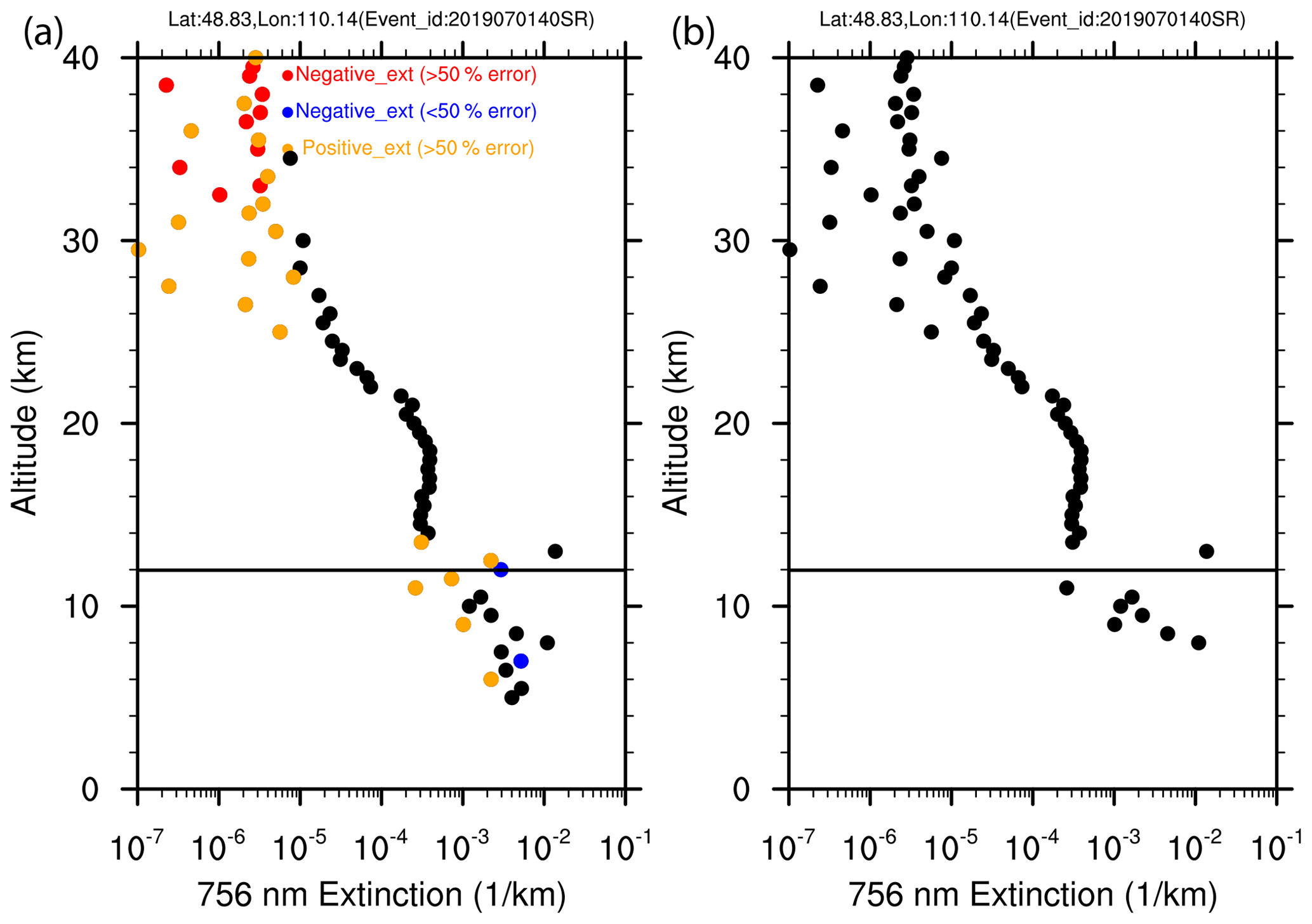
Figure 1 A sample extinction profile at 756 nm that shows negative extinction values in the lower stratosphere as well as in the troposphere (a). All extinction values are plotted as absolute values, and negative extinction values are color coded using red (blue) filled circles with >50 % (<50 %) error, whereas orange symbols represent positive extinction with >50 % error. The black dots represent positive extinction coefficients with <50 %. Panel (b) shows the absolute extinction profile after filtering negative values. The absolute values of the negative extinction coefficients (blue and red dots) are plotted to accommodate the log scale. The horizontal line represents the tropopause height.

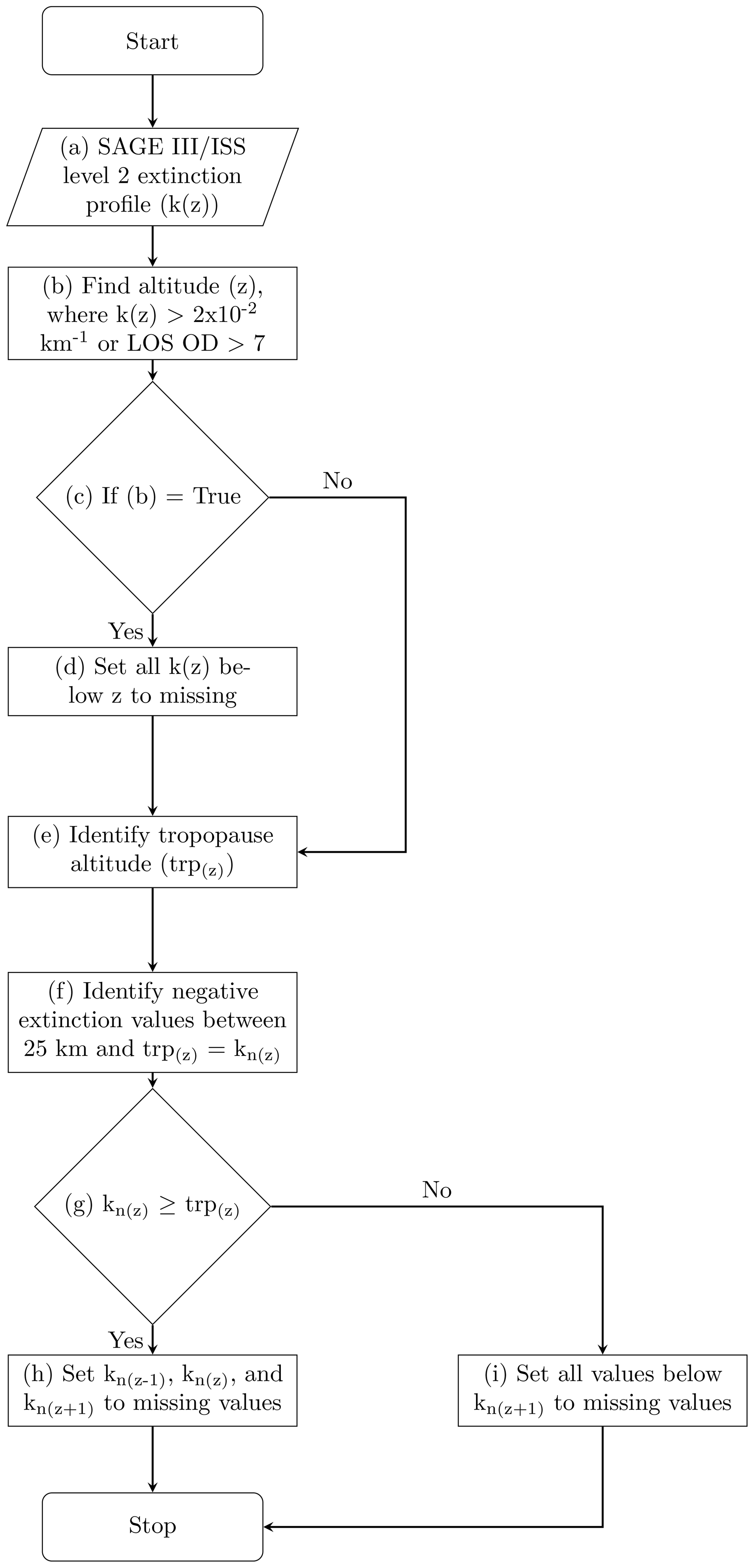
Figure 2 Flowchart of the negative extinction coefficient filtering method. k_(z) in the flowchart represents the extinction coefficient at altitude z, and panels (a) through (i) represent steps involved in the filtering algorithm.

3.2 TV13^* method

The TV13^* method uses the 525 to 1020 nm extinction ratio to separate between aerosol and aerosol–cloud mixtures. This is possible because the 525 and 1020 nm extinction efficiency kernels (Q_(λ,r), where Q is extinction efficiency, λ is the wavelength, and r is the radii) and resulting extinction coefficients show significant variations across particle sizes normally observed in the stratosphere. Extinction ratio was computed theoretically from aerosol extinction efficiency using Mie theory (assuming a lognormal distribution and 75 % sulfuric acid composition; Rosen, 1971; Steele and Hamill, 1981; Palmer and Williams, 1975). Figure 3a shows the extinction efficiency for SAGE II and III aerosol channels with the ratios of 521 to 1020 nm and 756 to 1544 nm shown in Fig. 3b. The variations with particle radius in Fig. 3b show that at larger particle sizes, the dependence on radius becomes invariant so that above a particle size of about 0.5 µm, all particles have essentially the same 525:1020 extinction ratio. Under most circumstances, particles of this size, or extinction ratios close to 1, are due to the presence of cloud. However, material from intense volcanic eruptions like Mt. Pinatubo or ash can produce similar ratios (e.g., SPARC, 2006; Legras et al., 2022). Furthermore, smoke, which often has a roughly gray spectral dependence, can also produce low extinction ratios in the measurements. In TV13, this was applied to a period of low extinction levels observed between 1999 and 2005. For our modified TV13^* approach, we use SAGE III/ISS data collected that include numerous aerosol perturbations. We also use the anomalous negative value process described above in Sect. 3.1. In addition, we divide the SAGE III/ISS data by month rather than season to facilitate comparisons with the SOATCM (see Sect. 3.4) that will be monthly based due to implementation issues associated with the SAGE III mission.

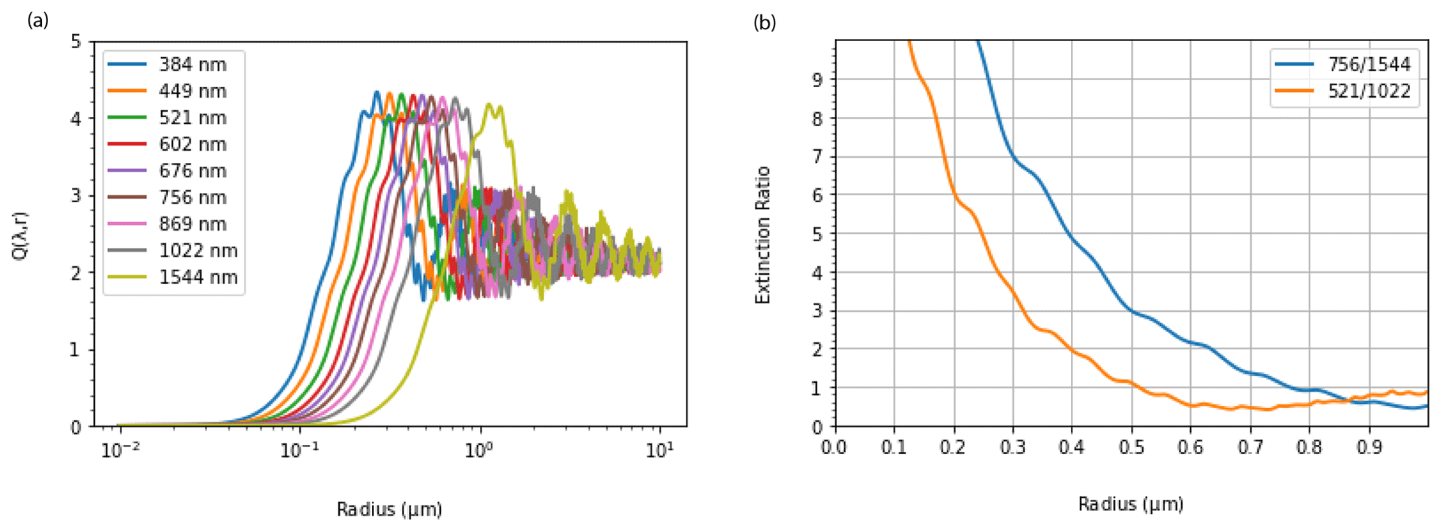
Figure 3 Panel (a) shows Mie extinction efficiency kernel (Q_(λ,r), where Q is extinction efficiency, λ is the wavelength, and r is the radii) as a function radius for all SAGE III/ISS wavelengths. Panel (b) shows extinction ratios of $\mathrm{521}/\mathrm{1022}$ and $\mathrm{756}/\mathrm{1544}$ computed using extinction kernels from panel (a) as a function of radii.

Figure 4 shows a scatter plot of the 525:1020 nm extinction ratio (r_525:1020) as a function of 1020 nm extinction for February during the period 2017 through 2021 at an altitude of 15 km. Figure 4 shows a long arm of data that stretch from the aerosol centroid with an extinction ratio of 3.5 and an extinction coefficient of $\mathrm{2.24}\times {\mathrm{10}}^{-\mathrm{4}}$ toward an extinction ratio of 1 (aerosol centroid is computed using median of the data and is described in detail in Sect. S1 in the Supplement). While a theoretical $r_{\mathrm{525}:\mathrm{1020}}=\mathrm{1.0}$ is used to filter out clouds based on Fig. 3b, an offset of 0.4 is used, following TV13, to account for the spread we observe in the tail of the scatter plot as the extinction ratio approaches unity. We therefore use $r_{\mathrm{525}:\mathrm{1020}}=\mathrm{1.4}$ as the threshold for separating pure aerosol and aerosol–cloud mixture. The rationale for using $r_{\mathrm{525}:\mathrm{1020}}=\mathrm{1.4}$ is further discussed in the Supplement (Sect. S1).

Figure 4 Scatter plot of extinction ratio ($\mathrm{525}/\mathrm{1020}$) as a function of the 1020 nm extinction coefficient for February at 15 km altitude. Global data between 2017 and 2021 are used for the plot. Vertical and horizontal red lines show k_0TV13 and $r_{\mathrm{525}:\mathrm{1020}}=\mathrm{1.4}$ respectively.

The TV13^* classification process is shown in Fig. 5 and described below.

• We use SAGE III/ISS extinction coefficient data (after screening negative values) as input (box a in Fig. 5).

• As a next step toward aerosol and aerosol–cloud mixture classification for the TV13^* method, we compute the 525:1020 nm extinction ratios (r_525:1020) (see box b, Fig. 5).

• The next step is to compute an absolute-deviation-based statistic k_0TV13 (defined as $k_a+{\mathrm{3.0}}^{*}\text{MAD}$, where k_a is the median extinction coefficient and MAD is the median absolute deviation). This is shown in Fig. 5c and plotted as a red vertical line in Fig. 4 (k_0TV13 is computed following TV13 by using extinction measurements with $r_{\mathrm{525}:\mathrm{1020}}>\mathrm{2}$).

• The next step is to isolate extinction coefficients (k_(z,λ), where k is the extinction coefficient at altitude z and wavelength λ) with $r_{\mathrm{525}:\mathrm{1020}}>\mathrm{1.4}$ (box d, Fig. 5).

• We then use k_(z,λ) and k_0TV13 to identify perturbed aerosol. If $k_{(z,\mathit{\lambda })}>k_{\mathrm{0}\text{TV13}}$ (Fig. 5e), then k_(z,λ) is flagged as “perturbed aerosol” as shown in Fig. 5f. This is also shown in Fig. 4 as data to the right of the red vertical line in the upper-right quadrant.

• The next step is to isolate the extinction coefficients k_(z,λ) with $r_{\mathrm{525}:\mathrm{1020}}<\mathrm{1.4}$. If $k_{(z,\mathit{\lambda })}>k_{\mathrm{0}\text{TV13}}$ with $r_{\mathrm{525}:\mathrm{1020}}<\mathrm{1.4}$ (Fig. 5g), then k_(z,λ) is flagged as an “aerosol–cloud mixture” as shown in Fig. 5h. This is also shown as data in the lower-right quadrant in Fig. 4.

• We then use k_(z,λ) with $r_{\mathrm{525}:\mathrm{1020}}>\mathrm{1.4}$ to classify standard aerosol. If $k_{(z,\mathit{\lambda })}<k_{\mathrm{0}\text{TV13}}$, then k_(z,λ) is flagged as “standard aerosol” as shown in Fig. 5i. This is also shown in Fig. 4 as data to the left of the red vertical line in the upper-left quadrant.

• The next step is to use extinction coefficient k_(z,λ) with $r_{\mathrm{525}:\mathrm{1020}}<\mathrm{1.4}$ to identify standard aerosol. If $k_{(z,\mathit{\lambda })}<k_{\mathrm{0}\text{TV13}}$, then k_(z,λ) is flagged as standard aerosol as shown in Fig. 5j. This is also shown in Fig. 4 as data to the left of the red vertical line in the lower-left quadrant.

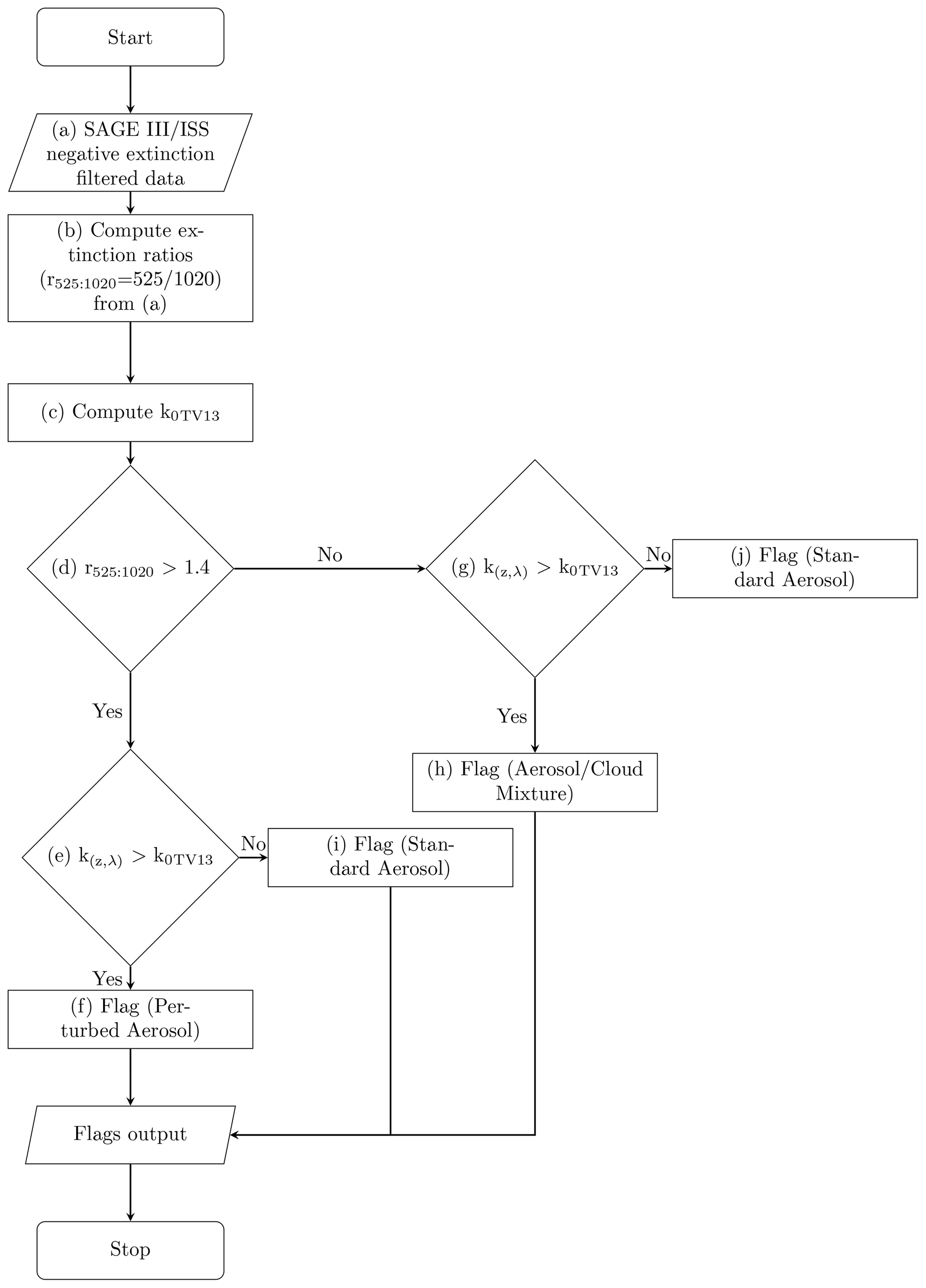
Figure 5 Flowchart of the TV13^* method. k_(z,λ) in the flowchart represents the extinction coefficient at altitude z and wavelength λ, whereas $k_{\mathrm{0}\text{TV13}}=k_a+{\mathrm{3.0}}^{*}\text{MAD}$. k_0TV13 is computed following TV13 by using extinction measurements with $r_{\mathrm{525}:\mathrm{1020}}>\mathrm{2}$. It should be noted that the steps involved (panels b through j) in the flowchart are the same as TV13 method, except that the seasonal data between 1999 and 2005 were used for the method presented in TV13. For our analyses, instead of seasonal data, we use monthly data collected between 2017 and 2021.

TV13 had also used an empirical model based on aerosol centroid, as well as an artificial cloud centroid with extinction ratio of 1.4 and an extinction coefficient of 10⁻¹ km⁻¹ to fit the data. A detailed description of the empirical TV13^* model is available in Sect. S1.

3.3 Perturbed stratosphere and the SOATCM

The SOATCM is similar to the TV13^* method above. However there are several changes which are outlined below and summarized in Fig. 7. The first change is the aerosol extinction coefficient wavelengths used in the process. While the approach used by the TV13^* method was based on the 525:1020 nm extinction ratio, we used the 756:1544 nm extinction ratio for the SOATCM. The rationale for using the 756:1544 nm wavelength combination is threefold: (1) the SAGE III/ISS 521 nm aerosol extinction measurement is subject to known artifacts; (2) the 756 and 1544 nm wavelength pair are about a factor of 2 different (comparable to the 525:1020 nm ratio used in TV13 for SAGE II); and (3) unlike the 525:1020 nm extinction ratio, the 756:1544 nm extinction ratio extends particle size differentiation to large sizes. Figure 3b shows the theoretical 756:1544 ratio as a function of particle size and demonstrates that the ratio retained sensitivity to particle size changes up to ≈0.8 µm rather than 0.5 µm for the 525:1020 nm ratio. Therefore, the 756:1544 wavelength combination allows size discrimination at lower altitudes in the lower troposphere where larger aerosol particles can be observed following volcanic eruptions (e.g., ash), and we used the 756:1544 extinction ratio for the SOATCM proposed here.

SAGE III/ISS has borne witness to a number of moderate eruptions and several PyroCb events that reached the stratosphere (see Table 1). Given the frequency of events that enhance the aerosol extinction, it is challenging to employ a cloud-screening algorithm for SAGE III/ISS based solely on the presence of outliers without a substantial risk of denoting volcanic or smoke-related enhancements as “cloud”. In developing the SOATCM, we found it critical to identify instances of enhanced aerosol within the observations and track that enhancement as it dissipates. Median absolute deviation statistics are computed on a monthly basis with a 20^∘ latitude band that is centered at the volcanic/fire event latitude. We then define an outlier extinction coefficient from the monthly probability density function distribution. Following Iglewicz and Hoaglin (1993), we define an outlier extinction coefficient, k₀, as $k_a+{\mathrm{3.5}}^{*}\text{MAD}$, where k_a is the median extinction coefficient and MAD is the median absolute deviation. Figure 6 shows a time series of k₀ for 1544 nm for various latitude bands for all events shown in Table 1, with points we consider enhanced denoted in red. Based on the k₀ time series, the time frame of the volcanic/fire event is determined. k₀ is an estimate of the extreme value that represents the enhancement of the extinction coefficient due to any volcanic/fire event. The altitudes are chosen in such a way that they represent average tropopause altitude for each latitude band. The computation of time series step is shown as box (b) in the flowchart (Fig. 7).

Table 1 Volcanic and PyroCb events used in this study.

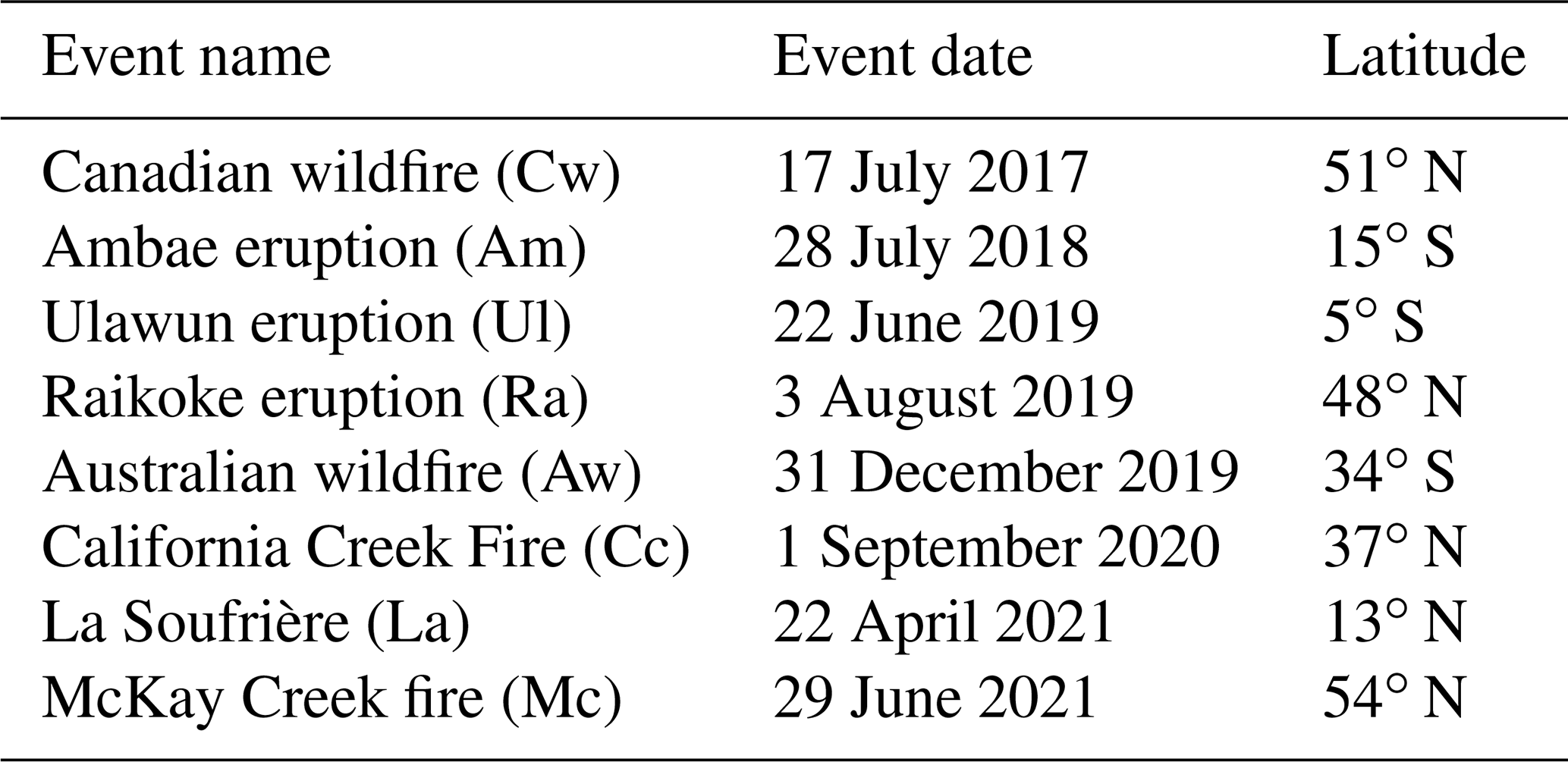
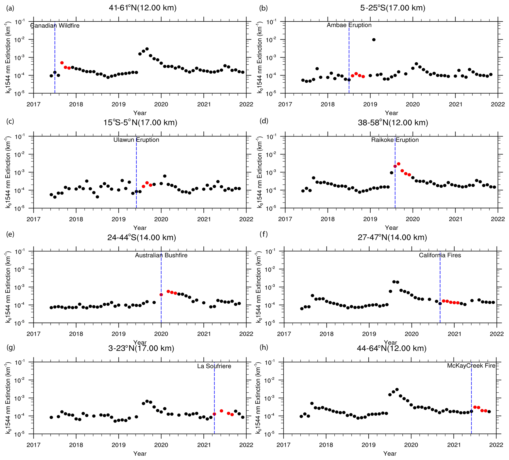
Figure 6 Time series of k₀ 1544 nm extinction for different latitude bands. Red symbols show the time line of the enhanced aerosol extinction coefficient and the time it takes to get back to the standard aerosol level following each event. The panels show events listed in Table 1: (a) Canadian wildfire, (b) Ambae eruption, (c) Ulawun eruption, (d) Raikoke eruption, (e) Australian wildfire, (f) California Creek Fire, (g) La Soufrière, and (h) McKay Creek fire. The altitudes shown in figure are the averaged tropopause altitude for the respective latitude band.

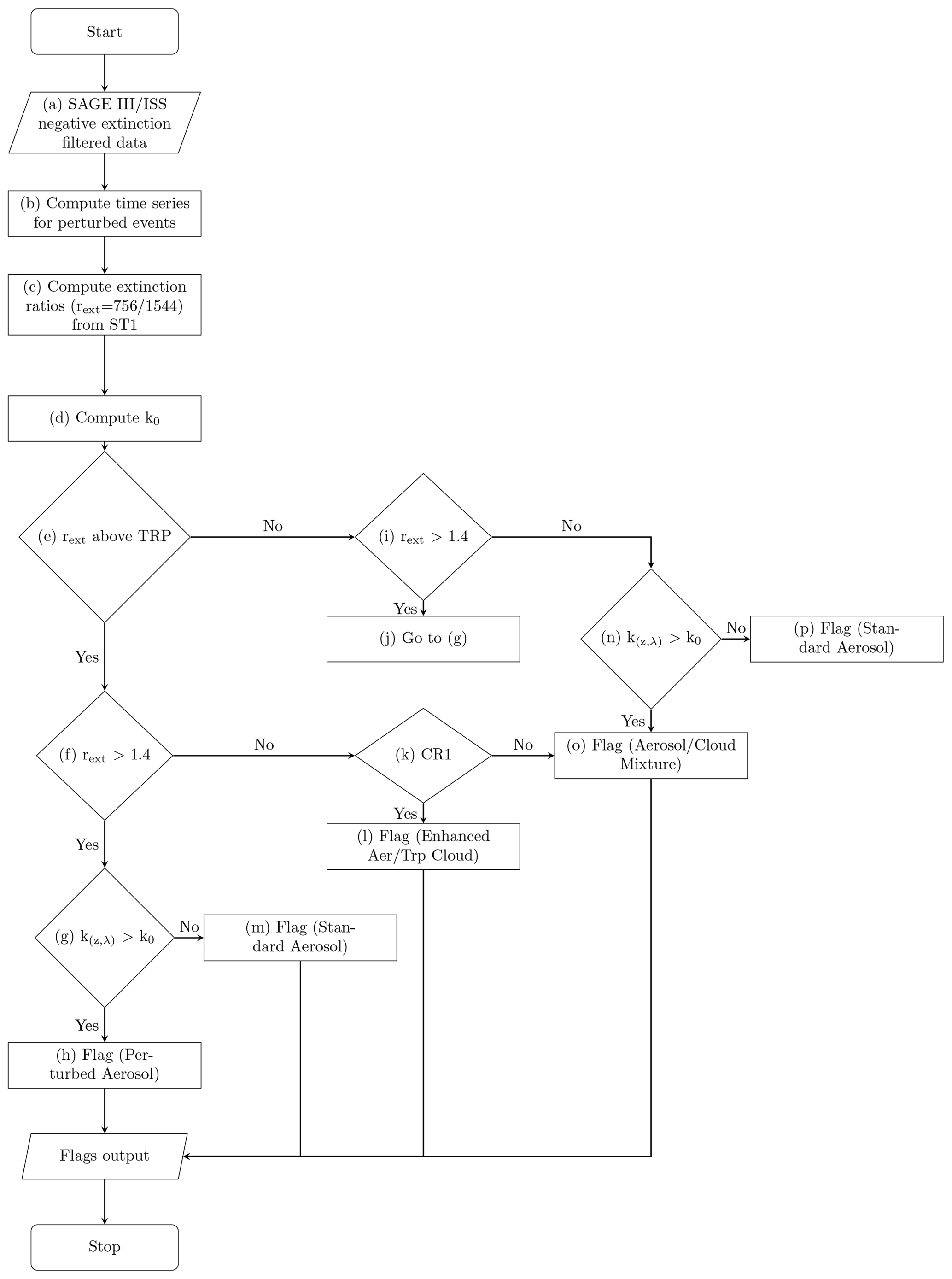
Figure 7 Flowchart of the SAGE III/ISS Operational Aerosol Type Classification Method. k_(z,λ) in the flowchart represents the extinction coefficient at altitude z and wavelength λ, whereas $k_{\mathrm{0}}=k_a+{\mathrm{3.5}}^{*}\text{MAD}$. TRP in the flowchart represents tropopause altitude, and panels (a) through (p) represent steps involved in the algorithm. The influence of the perturbed event on extinction is decided based on whether an extinction coefficient data point falls within the prescribed latitude band which is based on a perturbed event (Fig. 6) and whether the extinction ratio falls below 1.4. This is shown as CR1 in the flowchart.

Another difference between the TV13^* method and the SOATCM is that statistics for TV13^* are accumulated based on the global data set. However, for SAGE III/ISS, we noticed that the perturbed events cause inter-hemispheric differences in the data, leading to more than one cluster in the data. Figure 8 shows scatter plots of the extinction ratio versus extinction for two of the perturbed events. The upper panel of the figure shows how extinction ratios ($\mathrm{756}/\mathrm{1544}$) change with respect to 1544 nm extinction, following the Canadian wildfire event (∼ 51^∘ N) that occurred in August 2017, whereas the lower panel shows the same but for the Ambae eruption (∼ 15^∘S) in July 2018. While all of the data are plotted, we use different colors for different latitude bands to show the influence of any such event in the data. The data presented in Fig. 8 were plotted at two altitudes: 11 km (panels a–d) and 17 km (panels e–h). The 11 km altitude was chosen because it is approximately representative of the average tropopause height for this latitude band, and the 17 km altitude was chosen because it represents approximate tropopause altitude for the tropics. It is evident from the figure (panels a–d) that there is a distinct enhancement of the extinction coefficient in the northern latitude band (20–80^∘ N) following the Canadian wildfire event (Fig. 8b–d). Similarly, the lower panel shows data following the Ambae eruption in July 2018 and demonstrates distinctly enhanced extinction (Fig. 8f–h) from the southern latitude band (80–20^∘ S). Additionally, these global monthly data plots suggest there are inter-hemispheric differences in extinction ratios. Therefore, we divided monthly data into two latitude bands: (1) 80^∘ S–20^∘ N and (2) 20–80^∘ N. Initially, the tropical latitude band (20^∘ S–20^∘ N) was used as a separate band, but paucity of tropical data for statistical analysis forced us to combine the tropical latitude band with the southern latitude band (80–20^∘ S). Therefore, we perform aerosol categorization based on these two latitude bands (80^∘ S–20^∘ N and 20–80^∘ N), which is described in the following section.

Figure 8 Scatter plots of the 756 to 1544 nm extinction ratio versus 1544 nm extinction following the Canadian wildfire event in August 2017 (a–d) and the Ambae eruption in July 2018 (e–h). The upper panel shows scatter plots of the extinction ratio versus extinction at 1544 nm for August 2017 through November 2017 for an altitude of 11 km (a–d), whereas the lower panel shows the same but for August 2018 through November 2018 at 17 km.

Categorizing aerosols and aerosol–cloud mixtures

Figure 7 shows the flowchart for the SOATCM. The steps involved in categorizing aerosols/clouds using the SOATCM are described below.

• We use the SAGE III/ISS extinction coefficient data (after screening negative values) as input (Fig. 7a).

• The next step is to compute the time series (Fig. 6) to determine the influence of any perturbed event (Fig. 7b).

• We then compute the extinction ratios between 756 and 1544 nm (Fig. 7c).

• The next step is to compute monthly median absolute statistics (k₀) to estimate the outlier extinction coefficient. This is shown as Fig. 7d and as a vertical solid line in Fig. 9. It should be noted that k₀ is computed at each altitude.

• We then used r_ext and the tropopause height (TRP in Fig. 7) to separate data below and above the tropopause (Fig. 7e).

• An extinction ratio (r_ext) of 1.4 is then used as the threshold for separating aerosol and aerosol–cloud mixture due to the reasons mentioned above in the TV13^* method (while clouds nominally are expected to produce ratios of close to 1 in these measurements, many cloud observations are mixtures of aerosol and cloud, and thus ratios greater than 1 for observations that are inferred as cloud are common; the value of 1.4 is based on observations of the behavior of both SAGE II and SAGE III data sets). Data are treated differently whether they are above or below the tropopause. As a next step, we use data above the TRP and use extinction coefficients with r_ext>1.4 (Fig. 7f).

• If r_ext>1.4 and the extinction coefficient (k_(z,λ), where z is the altitude and λ is the wavelength) is greater than k₀ (Fig. 7g), then k_(z,λ) is flagged as perturbed aerosol (Fig. 7h). Figure 9 shows how the aerosol/cloud categorization is done by showing examples of two perturbed events: (a) the 2017 Canadian wildfire and (b) the 2018 Ambae eruption that occurred at ∼51^∘ N and ∼15^∘ S respectively. The perturbed aerosols are shown as pink filled circles in Fig. 9. The vertical red line in Fig. 9 represents k₀.

• We then look at the data below the tropopause and check if r_ext>1.4. If r_ext>1.4 is true, then the data are treated as stratospheric and the algorithm goes to step (g) as shown in Fig. 7j.

• If r_ext<1.4 and the data are above the TRP, then we use a different criterion (CR1). CR1 in Fig. 7k is dependent on the time series results from Fig. 6. We use enhanced extinction values (red filled circles) shown in Fig. 6 for each event and for a latitude band of 20^∘, centered at the latitude of occurrence. The influence of the perturbed event on extinction is decided based on whether an extinction coefficient data point falls within the prescribed latitude band which is based on a perturbed event and whether the extinction ratio falls below 1.4 based on Fig. 6. If the data fall within the time frame and latitude band of the perturbed event based on time series analysis (CR1 = true in Fig. 7), then we flag them as “enhanced aerosols/tropopause cloud” (Fig. 7l). These data points are shown as orange filled circles in Fig. 9. In contrast, these large particles (≥0.8 µm) with r_ext<1.4 and under background conditions are identified as an aerosol–cloud mixture, which may not be true under perturbed conditions (Fig. 9) where large particles could be enhanced aerosols, which could be misidentified as an aerosol–cloud mixture. While we use the time frame and latitude band of the perturbed event based on Fig. 6, a caveat on the enhanced aerosols/tropopause cloud flag is that these enhanced aerosols could be mixed with clouds or could just be clouds, particularly in the vicinity of the tropopause. We therefore use the enhanced aerosols/tropopause cloud flag rather than just enhanced aerosols so that the possibility of cloud is not completely overruled, particularly when the data fall in the region just above the tropopause.

• If r_ext>1.4 and the data are above the TRP with $k_{(z,\mathit{\lambda })}<k_{\mathrm{0}}$, the algorithm flags those data points as standard aerosol as shown in Fig. 7m. These data points can also be seen in Fig. 9 as green filled circles.

• If r_ext<1.4 and the data are below the TRP, then the algorithm checks if the extinction coefficient k_(z,λ) is greater than k₀ as shown in Fig. 7n. If $k_{(z,\mathit{\lambda })}>k_{\mathrm{0}}$, then k_(z,λ) is flagged as an aerosol–cloud mixture (Fig. 7o). This can also be seen in Fig. 9 as blue filled circles.

• Finally, if r_ext<1.4 and extinction coefficient k_(z,λ) (below the TRP) is less than k₀, then k_(z,λ) is flagged as standard aerosols (Fig. 7p). This can also be seen in Fig. 9 as green filled circles.

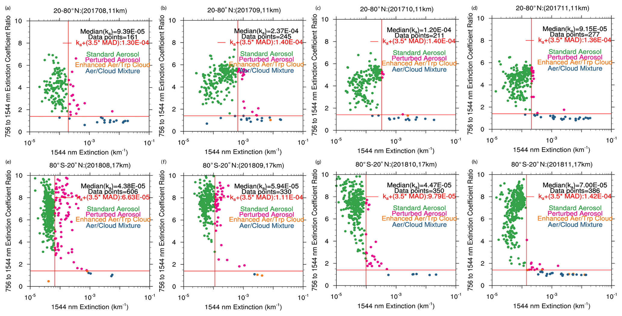
Figure 9 Scatter plots of the 756 to 1544 nm extinction ratio versus 1544 nm extinction following the Canadian wildfire event in August 2017 (a–d) and the Ambae eruption in July 2018 (e–h). The upper panels show scatter plots of the extinction ratio versus extinction at 1544 nm with aerosol/cloud categorization for August 2017 through November 2017 for an altitude of 11 km (a–d), whereas the lower panels show the same but for August 2018 through November 2018 at 17 km.

Additionally, we used an empirical model to fit the observed data, following the TV13^* method, which is also discussed in detail in Sect. S2.

3.4 Comparison between the TV13^* method and the SOATCM

Due to the limitations of the wavelength combinations (525:1020 nm) used in the TV13^* method as outlined in Sect. 3.2, there is a possibility that some of the larger aerosols (>0.5 µm) in the TV13^* method could be classified as aerosol–cloud mixture, particularly following a perturbed event. For the comparison between the TV13^* method and the SOATCM, we show profiles of the extinction coefficient at 1544 nm following two perturbed events. Figure 10 shows extinction coefficient profile plots at 1544 nm for two cases following the Canadian wildfire (upper panel) event and the Ambae eruption (lower panel) respectively.

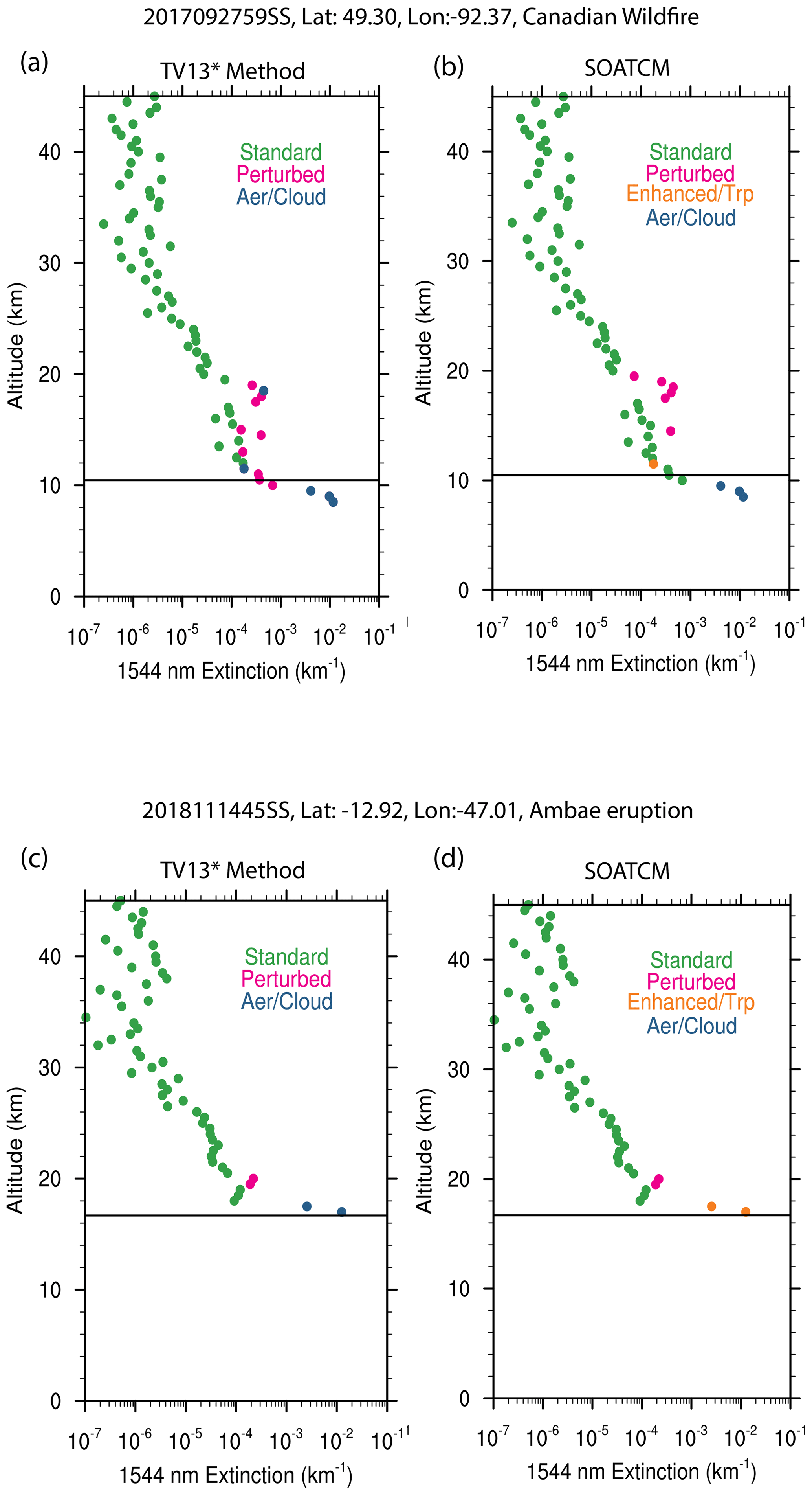
Figure 10 Aerosol/cloud categorization of extinction profiles at 1544 nm for the Canadian wildfire and the Ambae eruption. The upper panels show extinction profile comparison between the TV13^* method (a) and the SOATCM (b), following the Canadian wildfire, while the lower panel shows the same comparison but for a profile following the Ambae eruption. The event date for the profile for panels (a) and (b) is 27 September 2017 (latitude 49.30^∘ and longitude −92.37^∘), and for panels (c) and (d) it is 14 November 2018 (latitude −12.92^∘ and longitude −47.01^∘).

While there are some similarities between the two methods in categorizing standard and perturbed aerosols, there are differences that arise from the differing statistical methods and the differing wavelength combinations used in each method. While the TV13^* method works reasonably well in categorizing standard and perturbed aerosols based on long-term monthly statistics (all data collected between 2017 and 2021 for each month), the SOATCM uses month-to-month data to compute statistics and therefore is a better representation of categorization based on monthly statistics.

The important difference between the TV13^* method and the SOATCM is in categorization of enhanced aerosols/tropopause cloud. For the SOATCM, we use the influence of any perturbed event based on a time series as shown in Fig. 6 and use r_ext≤1.4 and $k_{(z,\mathit{\lambda })}>k_{\mathrm{0}}$ to identify enhanced aerosols/tropopause cloud. This categorization is made only above the tropopause altitude where the enhanced extinction coefficient with r_ext≤1.4 could occur as a result of a perturbed event. However, there could be a possibility of confusing with aerosols and clouds or just clouds at these altitudes. We do apply this category only when the above-mentioned criteria are met in the stratosphere. As a result, we retain these data points as enhanced aerosols/tropopause cloud. This can be seen in Fig. 10b for a profile that is influenced by the Canadian wildfire, and the enhanced aerosols/tropopause cloud categorization is made at 11.5 km (orange filled circle), whereas Fig. 10d shows the same but for the Ambae eruption at 17 and 17.5 km. It should be noted that for these two cases the TV13^* method flagged these data points as an aerosol–cloud mixture (Fig. 10a and c). Therefore, the important difference between the TV13^* method and the SOATCM is the way enhanced aerosols/tropopause cloud is treated. Additionally, for the TV13^* method an extinction ratio of 525:1020 nm (r_525:1020) was used, and therefore it is possible that larger particles with radii roughly >0.5 µm could be flagged as an aerosol–cloud mixture (based on Fig. 3b). Figure 10a shows one such case at 18 km, where the data are flagged as an aerosol–cloud mixture, whereas Fig. 10b flags that data point as perturbed aerosol. We provide several other cases of comparison between the TV13^* method and the SOATCM in the Supplement (Sect. S3), which shows similar results. Eventually, the SOATCM will be used to produce a level 3 SAGE III/ISS aerosol product.

For the SOATCM, in addition to the listed categorization, we make an effort to identify polar stratospheric clouds (PSCs) for the latitudes >55^∘ using a temperature-based filter. The PSCs are filtered out when the ambient temperature falls below 200 K (not shown here).

3.5 Application of the SOATCM to the Global Space-based Stratospheric Aerosol Climatology (GloSSAC)

Stratospheric aerosol is an important component in determining the radiative and chemical balance of the atmosphere. Many global climate models (GCMs) do not have an interactive aerosol module to treat stratospheric aerosol and therefore depend on global measurements on a long-term basis. Therefore, the Global Space-based Stratospheric Aerosol Climatology (GloSSAC) was created first in 2018 (Thomason et al., 2018) to support the climate modeling community for the Coupled Model Intercomparison Project Phase 6 (CMIP6) (Eyring et al., 2016). For GloSSAC, the SAGE series of measurements play a vital role in the long-term data starting from 1979 through present, excluding the post-SAGE II era (August 2005–May 2017) during which other space-based measurements were used to fill the gap (e.g., Thomason et al., 2018; Kovilakam et al., 2020). An important factor missing in those measurements was measurements of the extinction coefficient at multiple wavelengths. For GloSSAC version 2.0 (Kovilakam et al., 2020), we extended the data set to December 2018 with the inclusion of the SAGE III/ISS multiple wavelength data from June 2017. Recent changes in the stratospheric aerosol loading in the UTLS region have received significant attention in the scientific community (e.g., Bourassa et al., 2012; Vernier et al., 2015) as increased aerosol loading in this region can have a larger impact on radiative and chemical balance. Therefore, it is important to identify aerosols more accurately in the vicinity of the tropopause particularly following events that perturb the stratosphere.

For GloSSAC version 2.0 (v 2.0) (data product released in 2020 with data extended until 2018; Kovilakam et al., 2020), SAGE III/ISS aerosol extinction coefficient data have been incorporated with a simple extinction-ratio-based cloud filter approach (data with extinction ratio ($\mathrm{525}/\mathrm{1020}$ nm) >2.0 are only used as aerosols) to avoid any possible cloud contamination in the aerosol extinction data. By using this simple method, some enhanced aerosols from any perturbed event (e.g., volcanic eruptions, PyroCb events) may have been mistakenly flagged as clouds during SAGE III/ISS measurements, particularly in the vicinity of the tropopause and lower stratosphere. It is therefore important to address this issue in the aerosol data, particularly when it is used for a long-term climatology such as GloSSAC. Therefore, we incorporate the revised cloud-screening method described in Sect. 3.3 into the latest GloSSAC version 2.2 (v 2.2).

A detailed description of the various measurements used in constructing GloSSAC (v 2.0) is shown in Fig. 1 of Kovilakam et al. (2020). An interim version of GloSSAC was recently released (v 2.1) for which the new aerosol/cloud categorization described in Sect. 3.3 was implemented, without initial filtering of spurious negative values in the events as described in Sect. 3.1. In version 2.1 of GloSSAC, the data were extended to through 2020. We now extend data through 2021 as data from individual measurements became available for the year 2021. However, for the current version (v 2.2), there is no change in the individual measurements used, but there are version changes in each data set in addition to the cloud screening of SAGE III/ISS data as described above. The version changes of individual data sets are applicable only for the post-SAGE II era (September 2005–present) that now includes a version change in SAGE III/ISS data as described in Sect. 2, with version changes in Optical Spectrograph and InfraRed Imaging System (OSIRIS) and Cloud-Aerosol Lidar and Infrared Pathfinder Satellite Observation (CALIPSO) as described below.

We now use OSIRIS version 7.2 data compared to version 7.0 used in GloSSAC (v 2.0). For OSIRIS version 7.2, the background atmosphere was changed from ERA-Interim to MERRA2 re-analysis for consistency, and failures and missing data were also fixed so that there are now more scans in general. Overall, there are no significant differences between version 7.0 and 7.2, particularly above the UTLS region. Due to a decline in the coverage of the instrument, data for the month of June of 2018 through 2021 are now absent from the entire data set. Please note that due to inclusion of additional scans, the version 7.2 data now include an increased number of profiles compared to version 7.0, which also results in differences between version 7.0 and 7.2. These differences are apparent, particularly in the high-latitude bands. Additionally, in version 7.2, NO₂ regularization and ozone cross section have been changed (Adam Bourassa, personal communication, 2023).

CALIPSO aerosol backscatter measurements have been valuable for GloSSAC, particularly in filling the gaps in the measurements, mostly in the polar latitudes. We use CALIPSO's Cloud-Aerosol Lidar with Orthogonal Polarization (CALIOP) aerosol backscatter coefficient data, which have also undergone a minor change to version 1.01 from July 2020, which is due to a required upgrade to the operating system on the production cluster (https://www-calipso.larc.nasa.gov/resources/calipso_users_guide/data_quality/level_all_v001_20201002.php, last access: 4 March 2023). CALIOP data were available only until October 2021. We therefore used only the data that were available at the time of the analysis.

Here, we follow the methods described in Kovilakam et al. (2020) for merging OSIRIS, CALIOP, and SAGE III/ISS into the GloSSAC data set. For this version (v2.2) of GloSSAC, we update the data set post-2005, for which there are version changes on all three individual data sets that are used (i.e., OSIRIS, CALIOP, and SAGE III/ISS). While the measurements of OSIRIS and CALIOP provide most of the data in GloSSAC for the period from 2005 through mid-2017, it should also be noted that there are changes in instruments and fundamental changes in the measurements as noted previously (e.g., Thomason et al., 2018; Kovilakam et al., 2020). While OSIRIS and CALIOP instruments use a less direct technique compared to solar occultation, these instruments provide the greatest density of measurements. However, OSIRIS and CALIOP have challenges in retrieving aerosol properties. For OSIRIS, the retrieved aerosol extinction at 750 nm depends on an estimation of the aerosol scattering phase function, which is related to aerosol size distribution and composition. CALIOP's primary measurement is the backscatter coefficient which is measured at 532 nm. While CALIOP provides high-density measurements even in the polar latitudes, it appears to have poor precision on individual measurements in the stratosphere. Therefore, we use averaging of individual measurements to provide a precise product comparable to those provided by OSIRIS or SAGE when incorporating the data set into GloSSAC. Further, since the GloSSAC aerosol extinction coefficients are provided at 525 and 1020 nm, the conversion from the CALIOP backscatter coefficient to the extinction coefficient is another source of bias. A detailed description on biases related to individual instruments and their possible corrections is provided in Kovilakam et al. (2020).

3.5.1 Comparison of SAGE III/ISS data with OSIRIS

The primary wavelength at which the OSIRIS extinction coefficient is retrieved is 750 nm. Therefore, we need to convert the 750 nm extinction to the GloSSAC wavelengths which are at 525 and 1020 nm. Generally, the conversion to 525 nm is made using a constant Ångström exponent of 2.33 as noted in Rieger et al. (2015). While the comparison between OSIRIS and SAGE measurements is broadly in agreement, there appears to have been an overestimation of the OSIRIS extinction in the lower stratosphere when compared against SAGE II and SAGE III/ISS (e.g., Rieger et al., 2015; Thomason et al., 2018; Kovilakam et al., 2020). Figure 11 shows the zonally averaged monthly extinction coefficient percentage difference between OSIRIS and SAGE III/ISS for June 2017. For Fig. 11a, the OSIRIS extinction at 525 nm is computed using a constant Ångström exponent of 2.33, whereas in Fig. 11b the measurement is compared for 750 nm SAGE III/ISS measurement. Figure 11a and b show a reasonable agreement between OSIRIS and SAGE III/ISS except in the lower stratosphere and in the tropics where the percent difference exceeds 40 %. While Fig. 11a shows the same patterns as in Fig. 11b, the differences are significantly larger, which suggests either a deficiency in the conversion process of the OSIRIS extinction from 750 to 525 nm or SAGE III/ISS is biased low in the lower and middle stratosphere. Therefore, to maintain long-term consistency between data sets, it effectively requires that we bring OSIRIS in agreement with SAGE measurements. Following Kovilakam et al. (2020), a conformance process is performed to mitigate the differences between OSIRIS and SAGE measurements using a monthly climatology of the pseudo-Ångström exponent (the pseudo-Ångström exponent is derived using the monthly meanÅngström exponent as described in Kovilakam et al., 2020).

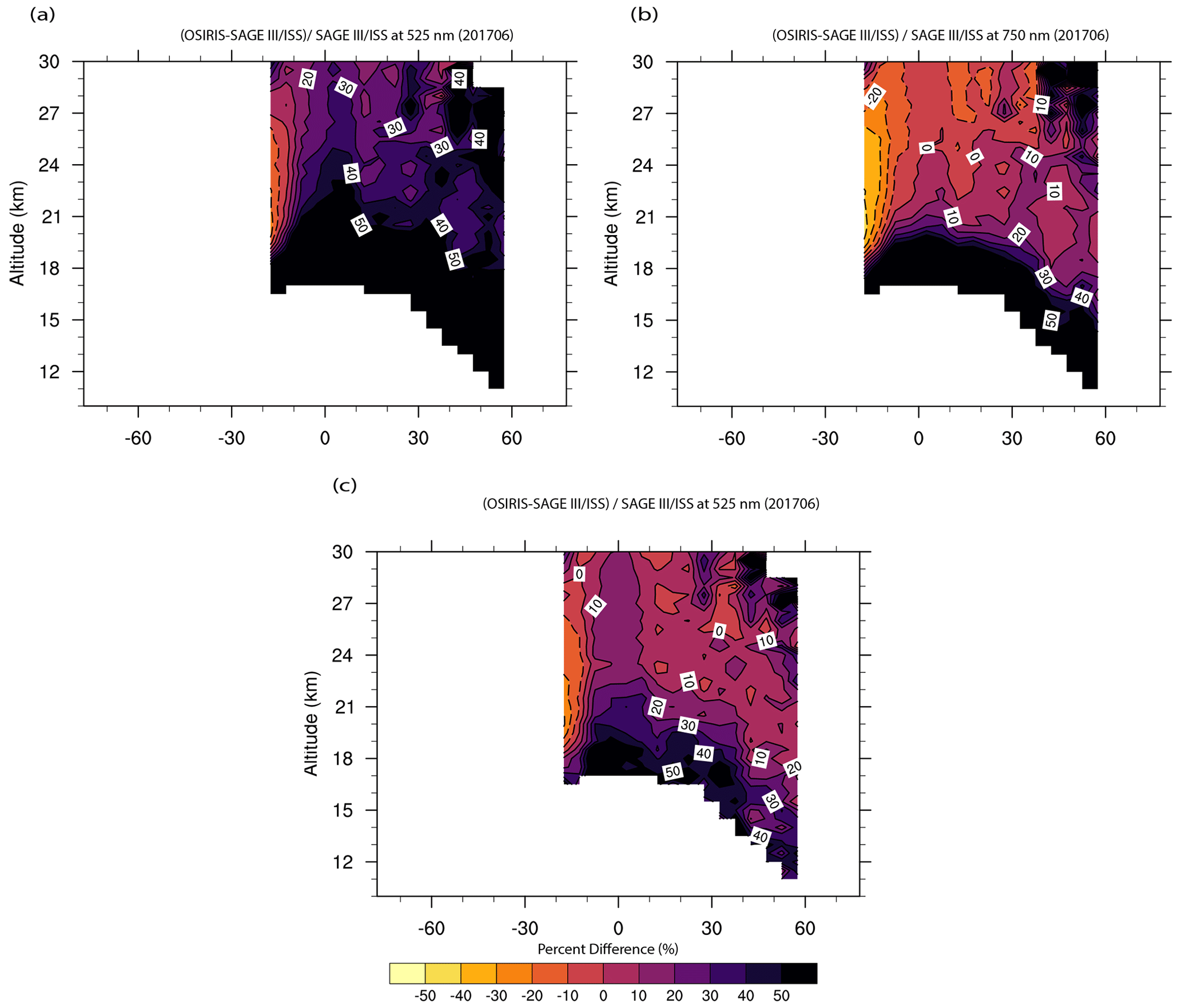
Figure 11 Percent difference between OSIRIS and SAGE III/ISS altitude versus latitude for June 2017 at (a) 525 nm and (b) 750 nm. An Ångström exponent of 2.33 is used to convert the OSIRIS extinction to 525 nm in panel (a) while a monthly climatology of the Ångström exponent from Fig. 12 is used to convert the OSIRIS extinction in panel (c).

While we follow the method provided in Kovilakam et al. (2020) for conforming OSIRIS data using pseudo-Ångström monthly climatology, it should be noted that we now include additional measurements available from OSIRIS and SAGE III/ISS from 2018 through 2021 to compute the monthly Ångström climatology. As noted in Sect. 3.5, there are version changes in both data sets that now introduce differences in the Ångström climatology, which is used for the conformance process. Figure 12 shows the pseudo-Ångström exponent monthly climatology on an altitude-versus-latitude basis, which was computed using 750 nm OSIRIS and 525 nm SAGE II and SAGE III/ISS data. The difference between Fig. 12 and Fig. 7 of Kovilakam et al. (2020) arises mostly due to the relatively less comparable data between OSIRIS and SAGE III/ISS for GloSSAC version 2.0, where OSIRIS did not have data processed for the year 2018. Here, we now have additional data available from January 2018 through December 2021 from both OSIRIS and SAGE III/ISS, and it should also be noted that both data sets have undergone small version changes, which may have also contributed toward the differences in Fig. 12 in comparison with Fig. 7 of Kovilakam et al. (2020). While the standard conversion of OSIRIS 750 to 525 nm uses a constant Ångström exponent of 2.33, Fig. 12 shows values range from 1 through 4 for much of the stratosphere with exceptions in the tropical lower stratosphere. It should be noted that the pseudo-Ångström exponent shown in Fig. 12 does not have any physical meaning as it accounts for potential deficiencies in both data sets, and it is simply a means to push the OSIRIS extinction measurements toward the measurements produced by SAGE. We therefore use pseudo-Ångström exponent data shown in Fig. 12 to convert the zonally averaged monthly extinction of 750 nm OSIRIS to 525 nm as shown in Fig. 11c.

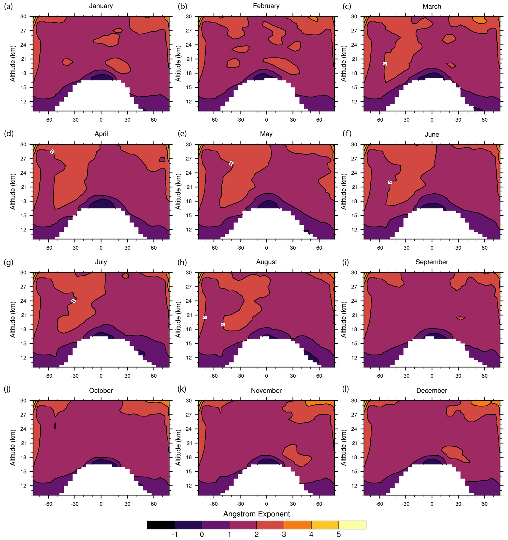
Figure 12 Altitude versus latitude of the Ångström exponent monthly climatology derived using OSIRIS 750 nm and the SAGE II and SAGE III/ISS 525 nm extinction. Outliers are removed using 3×3 median smoothing. Please note that we apply linear interpolation to fill in missing data that are mostly applicable for the polar latitude (poleward of 55).

Figure 11c shows the comparison between the bias-corrected OSIRIS and SAGE III/ISS measurements. Figure 11c shows a significant improvement of the OSIRIS extinction coefficient in the lower stratosphere where the differences are significantly reduced in comparison with Fig. 11a. While this agreement looks better in Fig. 11c for which the stratosphere is relatively less perturbed, there are some caveats as the usage of monthly climatology of the pseudo-Ångström exponent will be significantly different than the observed Ångström exponents, particularly following a perturbed event such as volcanic eruption or wildfire events. This becomes an issue for the period between SAGE II and SAGE III/ISS (August 2005 and June 2017) where we do not have any multi-wavelength measurements during which many small to moderate volcanic eruptions occurred.

Recently, it has been shown that many small to moderate eruptions were manifest during the SAGE II and III/ISS data record (Thomason et al., 2021). The size information inferred from the 525 to 1020 nm extinction ratios shows a decrease in the extinction ratio (increase in aerosol size) following large volcanic eruptions, whereas for small to moderate eruptions, extinction ratios are apparently slightly higher (smaller aerosol size) (Thomason et al., 2021). Therefore, we note that inferring aerosol size information for the post-SAGE II period (September 2005 through May 2017) is deficient, particularly following several small to moderate volcanic eruptions. We use monthly climatology of the pseudo-Ångström exponent for converting the OSIRIS extinction coefficient at 750 nm to 525 and 1020 nm as described in Sect. 2.4 of Kovilakam et al. (2020). While this conversion process is a better step forward in combining data sets into a uniform data set, the conversion process may be deficient in addressing evolving size changes that affect extinction measurements following any perturbed event (Kovilakam et al., 2020).

3.5.2 Comparison of SAGE III/ISS data with CALIOP and OSIRIS

Here, we follow the same method used in Kovilakam et al. (2020) to incorporate CALIOP data into the GloSSAC data set. While CALIOP uses lidar to measure the aerosol backscatter coefficient at 532 nm, a source of bias occurs when the backscatter coefficient is converted to the extinction coefficient as the conversion process requires information of unknown aerosol composition and size distribution (Kar et al., 2019). Here, we use the CALIOP standard stratospheric aerosol data product (Kar et al., 2019), with a minor version change from June 2020. For CALIOP data processing, a constant aerosol extinction-to-backscatter ratio of 50 sr is used (Kar et al., 2019) and the standard aerosol extinction is reported at 532 nm. Therefore, a constant Ångström exponent of 2.33 is used to convert the extinction coefficient to 525 nm. Figure 13a and b show percent differences between the standard CALIOP extinction coefficient and the bias-corrected OSIRIS and SAGE III/ISS extinction coefficient at 525 nm for November 2017. The CALIOP extinction in Fig. 13a and b is computed using a constant extinction-to-backscatter ratio of 50. CALIOP is in reasonable agreement with OSIRIS and SAGE III/ISS except in the lower stratosphere and at higher latitudes (>50^∘), where the differences are larger than 50 %. While we can attribute some of these differences in the northern higher latitudes to the PyroCb event associated with Canadian wildfire (Peterson et al., 2018), we note that similar differences persist even when the stratosphere is in the quiescent state. We therefore use a conformance method described in Kovilakam et al. (2020) to reduce the bias between measurements. Following Kovilakam et al. (2020), we implement an empirical scale factor (SF) which is computed as the ratio of the bias-corrected OSIRIS extinction at 525 nm to the CALIOP backscatter coefficient at 532 nm. As noted in Kovilakam et al. (2020), we re-derive the backscatter using the attenuated scattering ratio and molecular backscatter due to the fact that the standard aerosol backscatter coefficient is retrieved using a lidar ratio of 50 sr (Kar et al., 2019). For GloSSAC (v2.2), we use this alternate backscatter coefficient the same way as in Kovilakam et al. (2020).

Figure 13 Percent difference between the CALIOP, bias-corrected OSIRIS, and cloud-screened SAGE III/ISS extinction coefficients for November 2017. CALIOP data used in panels (a) and (b) are for 532 nm available in CALIOP stratospheric aerosol product, whereas CALIOP data in panels (c) and (d) are bias corrected using the scale factor (SF) shown in Fig.  14a.

Figure 14a depicts the annual median SF on an altitude-versus-latitude basis. Figure 14a suggests that the SF values range from 10 at polar latitudes to about 65 in the tropical high altitudes. While SF in Fig. 14a is in reasonable agreement with Fig. 9 of Kovilakam et al. (2020), the differences in Fig. 14 can be attributed to version changes and the additional measurements available from 2018 through 2021. Figure 14b shows the relative standard deviation for the SF in Fig. 14a and demonstrates that the SF is reasonably consistent except at polar latitudes where relative standard deviations are larger than 50 %. To compute the annual median SF, we use data from 2006 through 2021 when both measurements are available on a monthly basis. We then apply the conversion factors shown in Fig. 14a to the entire CALIOP data set on an altitude-versus-latitude basis. These empirically scaled CALIOP 525 nm data are used for computing the percent difference plots shown in Fig. 13c and d. It is evident from these plots that the differences between the data sets are reduced and are mostly within ±20 % when compared against Fig. 13a and b, for which the difference was ≥50 %. While the discrepancies between the data sets are reduced, they are not completely eliminated. We follow the same approach for converting CALIOP backscatter from 532 to 1020 nm extinction (not shown here). We plan to revise this method in a future version of GloSSAC as a time-dependent SF can possibly be introduced after filling in missing values of OSIRIS and CALIOP monthly data using equivalent latitude.

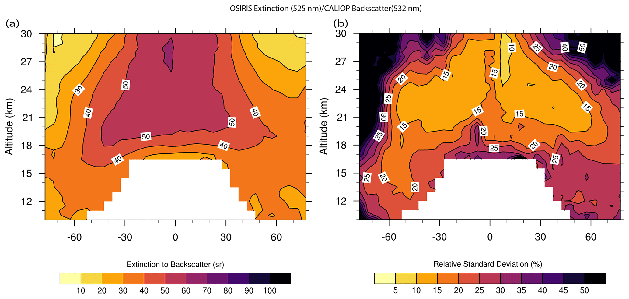
Figure 14 (a) Altitude-versus-latitude dependence of the 525 nm bias-corrected OSIRIS extinction to 532 nm CALIOP backscatter ratio (SF) for the overlap period between 2006 and 2021. (b) The relative standard deviation of panel (a) is computed at each grid point with respect to the median value in percent.

4 Implications of cloud screening on GloSSAC

For GloSSAC, SAGE III/ISS data are zonally averaged into 5^∘ latitude bins and 0.5 km altitude resolution on a monthly basis and incorporated into GloSSAC. Additionally, for version (v2.2), we perform a linear interpolation along the time axis to fill in missing values at higher latitudes. For a future release, we plan to implement a reconstruction method for SAGE III/ISS to fill in missing data – a method similar to the one used for SAGE II in GloSSAC version 1.0 (Thomason et al., 2018). It should also be noted that we now use version 5.2 SAGE III/ISS products in GloSSAC v2.2 with the revised cloud-screening algorithm, whereas SAGE III/ISS version 5.1 was used in GloSSAC v2.0 (Kovilakam et al., 2020). Figure 15 shows the impact of the revised cloud-screening algorithm on SAGE III/ISS aerosol data. For the cloud-screened product, we use three flags from the cloud-screening algorithm, which are standard aerosol, perturbed aerosol, and enhanced aerosol/tropopause cloud respectively as shown in Sect. 3.3.1. It should also be noted that, while we use the 756 and 1544 nm wavelength extinction ratio for the aerosol/cloud categorizations, the categorizations mentioned in Sect. 3.3.1 are applied to all aerosol channels from 384 through 1544 nm on the basis of the $\mathrm{756}/\mathrm{1544}$ nm extinction ratio. GloSSAC provides zonally averaged extinction coefficients at 525 and 1020 nm wavelengths for historical reasons. We therefore continue the same historical measurement wavelengths in the latest version of GloSSAC v2.2. While we note the negative bias in the 525 nm channel, a correction has been made to the 525 nm channel by spectrally interpolating extinction between the 450 and 756 nm channel using the Ångström exponent (Knepp et al., 2022). It should also be noted that the bias between measured and Ångström exponent interpolated values due to the curvature in the spectra is generally within ±10 % (Thomason et al., 2010).

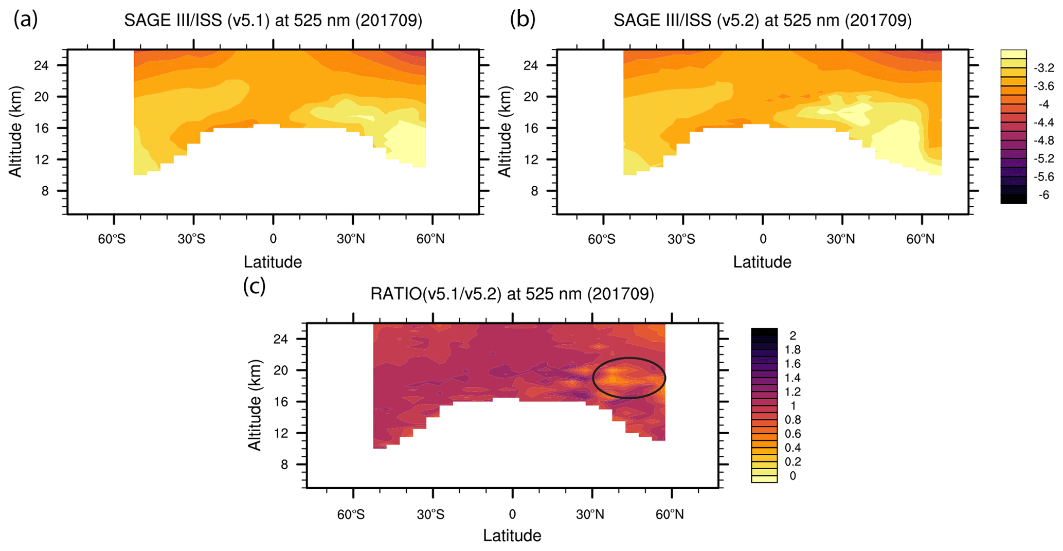
Figure 15 Zonally averaged SAGE III/ISS altitude-versus-latitude extinction coefficients for September 2017 following the Canadian wildfire event. (a) Version 5.1, (b) version 5.2, and (c) ratio between version 5.2 and 5.1. Extinction coefficient values are shown in the log to base 10.

Figure 15a and b show zonally averaged altitude-versus-latitude plots of extinction coefficients at 525 nm for version 5.1 and 5.2 respectively. The impact of cloud screening is evident from Fig. 15b, with a clear enhancement in the extinction coefficient in the latitudes >30^∘ N, particularly in the lower stratosphere. The enhanced extinction in version 5.2 is further evident from Fig. 15c, which shows the ratio of the extinction coefficient between version 5.1 and 5.2. Figure 15c shows lower range of ratios from 0.40 to 0.6, between 37.5 and 57.5^∘ N latitudes and at altitudes between 17 and 19 km (marked with a black oval in Fig. 15c). Lower ratios suggest an enhanced extinction coefficient in version 5.2, which occurs due to the removal of extinction coefficient data points with extinction ratios ≤2.0 in version 2.0. Additionally, for version 5.2, we perform a linear interpolation along the time axis to fill in missing values at higher latitudes, which can be seen in Fig. 15b.

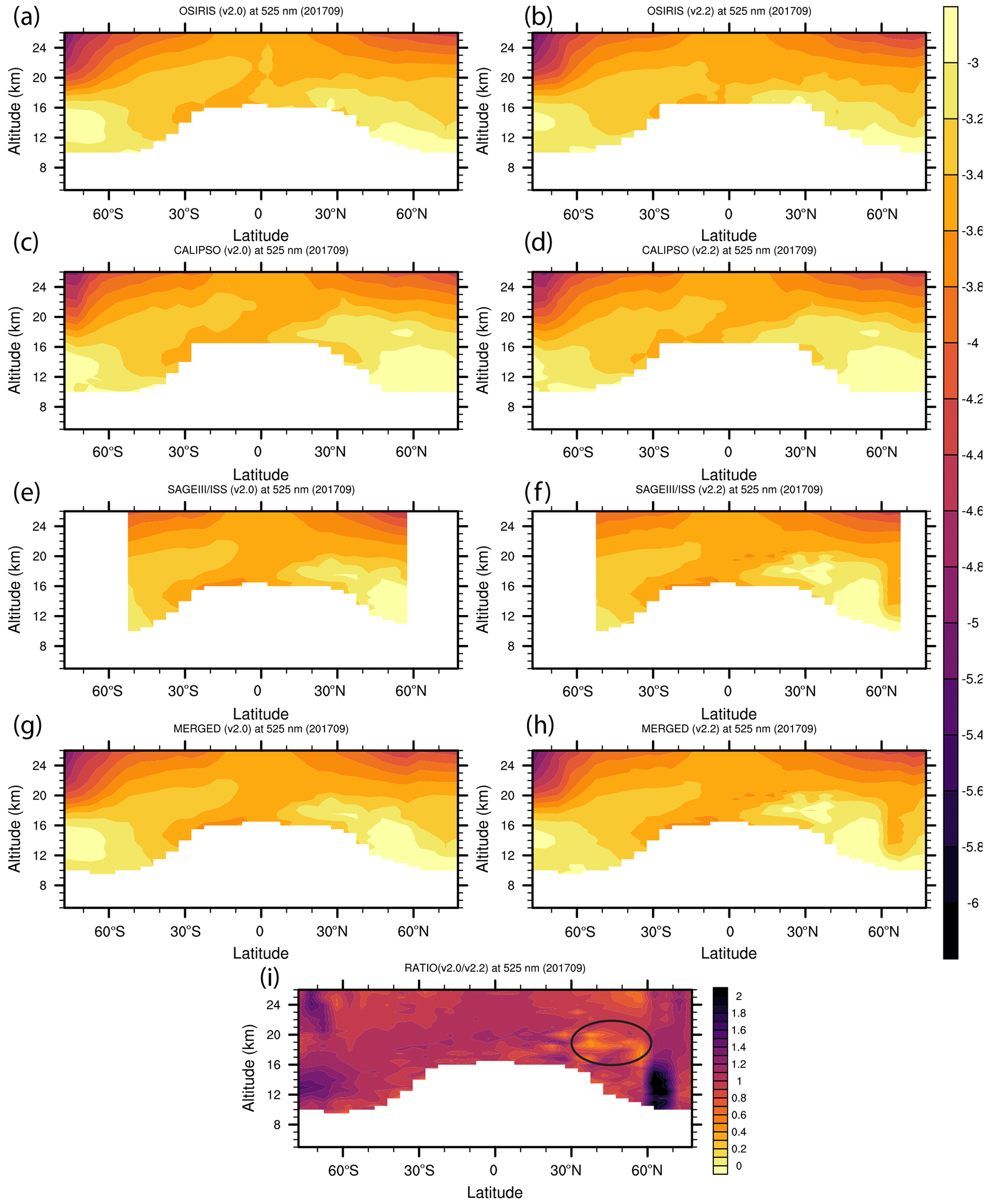
Figure 16 Altitude-versus-latitude dependence of 525 nm extinction for September 2017. Panels (a), (c), (e), and (g) are for OSIRIS, CALIOP, SAGE III/ISS, and merged extinction for version 2.0 respectively, whereas panels (b), (d), (f), and (h) are for version 2.2. Panel (i) shows the ratio between merged version 2.2 (h) and 2.0 (g).

4.1 Comparison of GloSSAC version 2.2 with version 2.0

To construct the GloSSAC data set, all individual measurements are gridded to the GloSSAC resolution (monthly, 0.5 km altitude and 5^∘ latitude resolution). As previously done for GloSSAC v2.0, from June 2017, we prioritize SAGE III/ISS data over OSIRIS and CALIOP. For the post-2017 data, several small to moderate volcanic events and a few large wildfire events have been reported (Table 1). It is therefore important to compare the differences between version 2.2 and version 2.0 of the GloSSAC data set. Figure 16 shows the extinction coefficient for September 2017, following the Canadian wildfire, for version 2.0 and 2.2, as well as the ratios. It is evident from Fig. 16i that the revised cloud-screening method used in v2.2 retains extinction data in the lower stratosphere that were otherwise removed in version 2.0 because of a simple extinction ratio filter – thereby enhancing aerosol extinction in version 2.2 for the latitude band between 35 and 50^∘ N for altitudes between 17 and 19 km (marked with a black oval in Fig. 16i). Lower ratios in Fig. 16i suggest an enhanced extinction coefficient in version 2.2, which occurs due to the removal of extinction coefficient data points with extinction ratios ≤2.0 in version 2.0. The differences we see in Fig. 16i are the same as in Fig. 15c for the latitudes between 50^∘ S and 50^∘ N, for which SAGE III/ISS data are used. The differences in the polar latitudes (>60^∘) in version 2.2 could be attributed to changes that occurred in individual data sets in version 2.2 as shown in Fig. 16a–f. For the southern polar latitudes (poleward of 60^∘ S), the differences are mainly due to the version changes in the individual data sets, particularly from OSIRIS and CALIOP as shown in Fig. 16a–d. However, for the northern polar latitudes (poleward of 60^∘ N), the difference could be attributed to both version changes in the individual sets and a linear interpolation scheme performed for SAGE III/ISS data in GloSSAC v2.2 to fill in missing values.

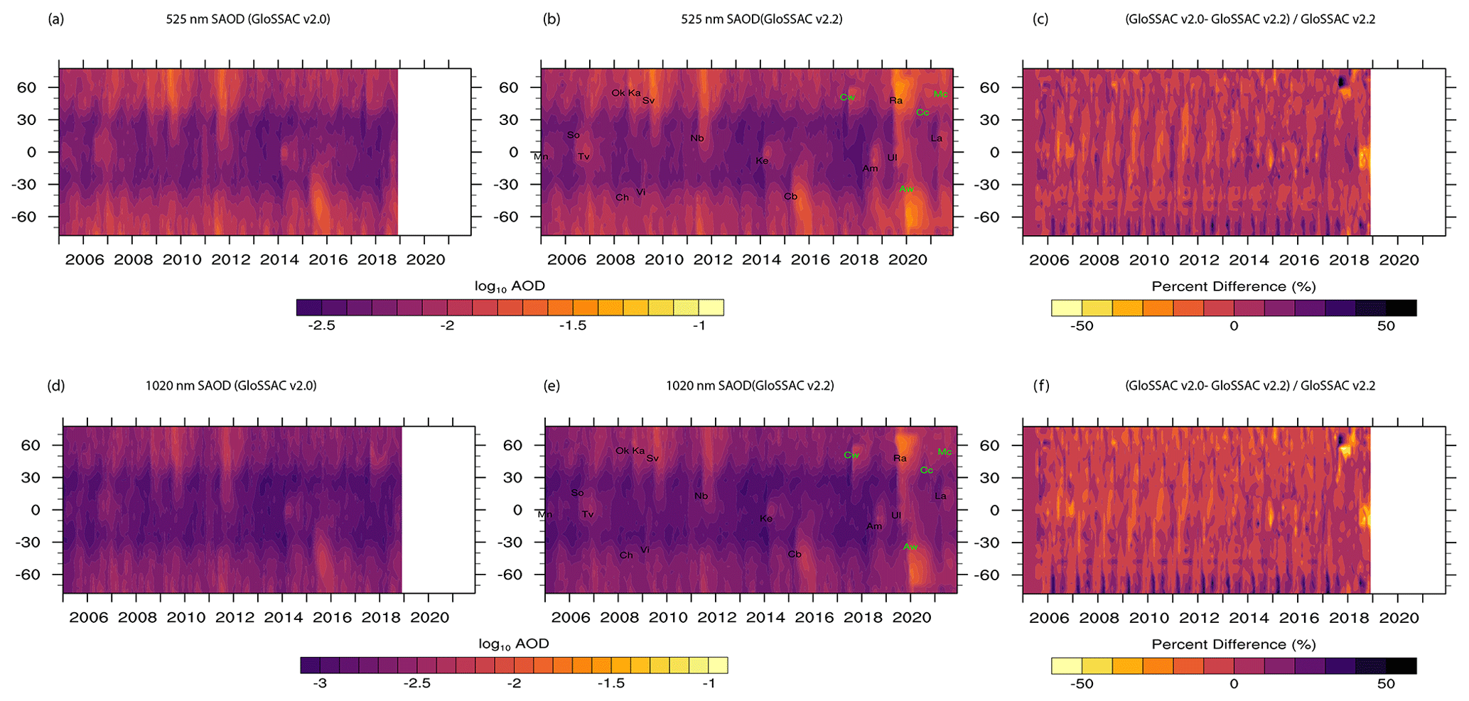
Figure 17 Latitude versus time dependence of stratospheric aerosol optical depth (SAOD) for 525 and 1020 nm. (a, b, c) SAOD for 525 nm for GloSSAC version 2.0, version 2.2, and percent difference between panels (a) and (b). (d, e, f) Same as in panels (a), (b), and (c) but for 1020 nm. (b, e) Major volcanic eruptions (black) and wild fire events (green) with abbreviated two-letter code with their respective latitude and time of occurrence that are listed here. The event names shown are Manam (Mn), Soufrière Hills (So), Tavurvur (Tv), Chaiten (Ch), Okmok (Ok), Kasatochi (Ka), Sarychev (Sv), Nabro (Nb), Kelut (Ke), Calbuco (Cb), Canadian wildfire (Cw), Ambae (Am), Ulawun (Ul), Australian wildfire (Aw), California Creek Fire (Cc), La Soufrière (La), and McKay Creek fire (Mc).

4.2 Stratospheric aerosol optical depth

Stratospheric aerosol optical depth (SAOD) was incorporated as a separate variable in all previous versions of GloSSAC, and therefore we incorporate SAOD into GloSSAC version 2.2. Figure 17 shows zonally averaged monthly latitude versus time of SAOD for GloSSAC version 2.0 and version 2.2. While the data in version 2.0 and 2.2 remain the same for the period prior to 2005, there are differences between the versions for the post-2005 time period. Therefore, we only show aerosol optical depth (AOD) changes post-2005 in Fig. 17. While the differences in SAOD at 525 and 1020 nm between version 2.0 and 2.2 are generally within ±20 % for latitudes between 60^∘ S and 60^∘ N, larger differences are noticeable in the high latitudes and the tropics, following the Canadian wildfire event in 2017 and the Ambae volcanic eruption in 2018 (Fig. 17c, f). The lower extinction coefficients in GloSSAC v2.2 in the polar latitudes could be attributable to the changes that occurred to individual data sets due to version changes. However, the enhanced extinction in GloSSAC (v2.2) followed by the Canadian wildfire event in July 2017 and Ambae volcanic eruption in 2018 is attributable to the new aerosol/cloud categorization in version 2.2 that retains lower stratospheric data, while GloSSAC version 2.0 used a simple extinction-ratio-based cloud filter that could have removed more aerosol data that have extinction ratios ≤2.0. While larger percent differences are observed following the Canadian wildfire in July 2017 for 1020 nm (percent difference as large as −52 % for the latitudes between 50 and 57.5^∘ N), a relatively smaller percent difference is observed for 525 nm (percent difference as large as −31 % for the latitudes between 50 and 57.5^∘ N). As far as the differences in the extinction coefficient following the Ambae volcanic eruption in July 2018 are concerned, both 525 and 1020 nm wavelengths show a larger percent difference in the tropical latitudes (percent difference is as large as −37 % (−47 %) for 525 nm (1020 nm), for the latitudes between 20^∘ S and 10^∘ N). However, these differences between version 2.0 and 2.2 are much lower (within 10 %) for globally averaged SAOD (Fig. 18). While the difference is much smaller in the globally averaged SAOD time series, Fig. 18b and d clearly show decreases in percent difference of SAOD following the Canadian wildfire event in July 2017 and the Ambae volcanic eruption in July 2018, suggesting higher extinction coefficients in version 2.2.

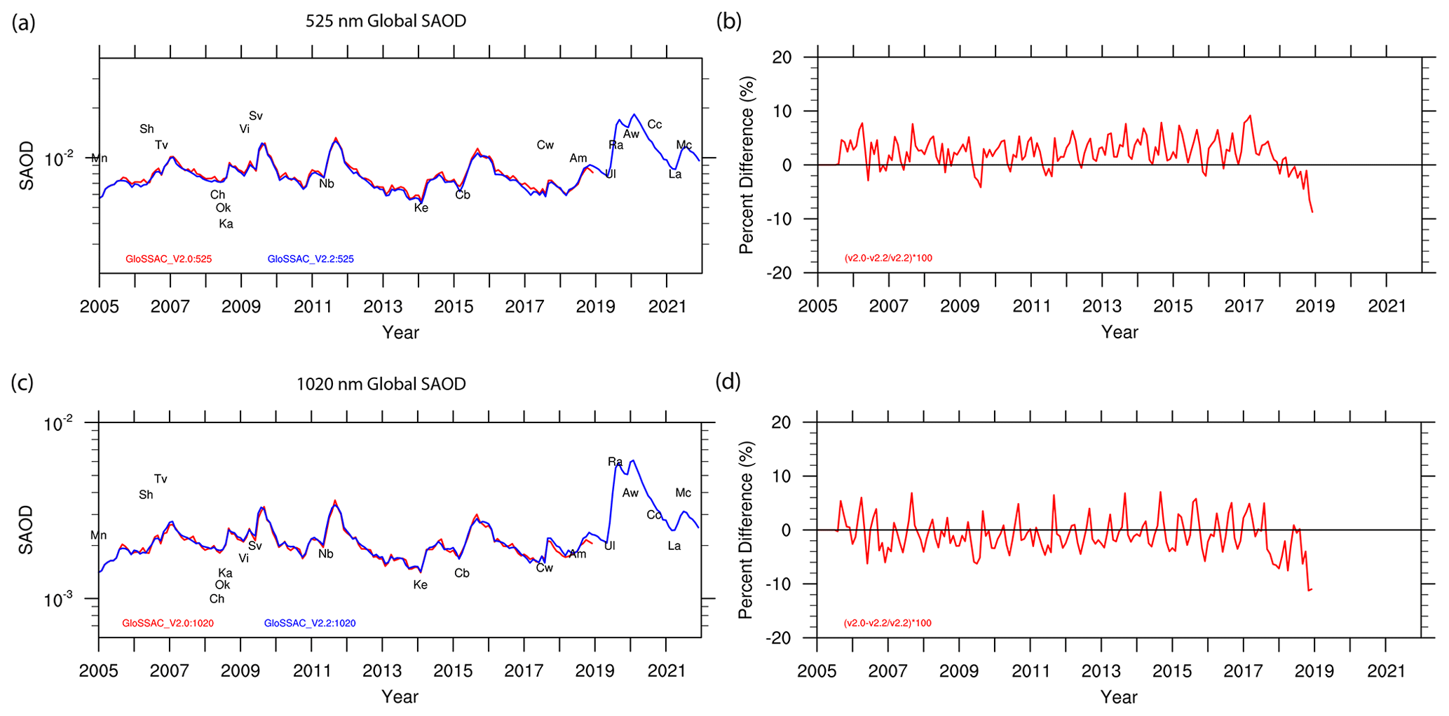
Figure 18 Time series of globally averaged SAOD for (a) 525 and (c) 1020 nm. The percent difference between version 2.0 and 2.2 is shown in panel (b) for 525 and panel (d) for 1020 nm.

5 Conclusions

We developed the SOATCM to categorize aerosol and clouds using SAGE III/ISS measurements. The primary goal behind the SOATCM was to account for the influence of recent volcanic eruptions and PyroCb events on stratospheric aerosol loading in SAGE III/ISS measurements. Eventually, the SOATCM will be used to produce a level 3 SAGE III/ISS aerosol product. The SOATCM works reasonably well for the periods during and following perturbed events such as volcanic/PyroCb. The influence of any perturbed activity in the stratosphere is estimated from the monthly time series of k₀, which is computed using median absolute deviation statistics and is now incorporated in the algorithm so that analyses that fall in this time frame are considered perturbed due to enhancement in k₀ value when compared against the standard aerosol. Additionally, we use temperature-based tropopause to classify the aerosols that are present in the vicinity of the tropopause which are otherwise flagged as an aerosol–cloud mixture.

The implications of the revised cloud-screening algorithm on GloSSAC data are also described. While there is no difference in the data prior to September 2005, the post-SAGE II era (September 2005–May 2017) clearly suggests differences between GloSSAC v 2.0 and this version (v 2.2). The differences between v2.0 and 2.2 are mostly attributable to version changes in the individual data sets, as well as the revised cloud-screening method used for SAGE III/ISS in v2.2 of GloSSAC. While all individual data sets for the post-SAGE II era underwent version changes, the changes to OSIRIS are perceptible due to the increased number of measurements in the latest version of OSIRIS (v7.1), which causes differences in the zonally averaged data for GloSSAC v2.2. While the differences are relatively low (≤20 %) except for the polar latitude for the period between the post-SAGE II era and the SAGE III/ISS era (June 2017–present), the difference between v2.0 and 2.2 of GloSSAC is relatively larger, particularly in the lower stratosphere following any perturbed events for the SAGE III/ISS time period (June 2017–present), which is attributable to the revised cloud-screening algorithm that now retains data in the lower stratosphere that were otherwise omitted with a simple extinction-ratio-based cloud screening in GloSSAC v2.0. The differences at the polar latitudes could be attributed to both version changes in individual data sets and the time interpolation of SAGE III/ISS data that is now implemented in version 2.2 due to discrepancies between data sets at the polar latitudes. While the same is true for SAOD where the time series of SAOD clearly shows the enhancement of SAOD following perturbed events, it is also noticeable that the enhancement of SAOD in the southern polar latitude that was present in all previous versions of GloSSAC is now diminished, although not completely. The improvements in SAOD in the polar latitudes could be attributable to increased number of measurements available in the latest version of OSIRIS (v7.2) and thereby improved zonal averaging for those latitude bands. Additionally, in GloSSAC v2.2, a time interpolation of SAGE III/ISS data is now implemented which may have caused some differences at the higher latitude as well. We also note that there are slight differences between the interim version 2.1 and this version (v 2.2) of GloSSAC (not shown here), as our aerosol/cloud categorization in both versions remains the same except that in version 2.2 an initial filtering of spurious negative values in the SAGE III/ISS events is implemented as described in Sect. 3.1. Additionally, in GloSSAC 2.2, the OSIRIS version changes from 7.1 to 7.2.

While there are noticeable improvements in GloSSAC v2.2, we plan to implement some changes in the future that are listed below.

• We plan to revisit the way smoke events are represented in GloSSAC during the SAGE II era. We plan to consider the possibility of not using any cloud clearing for SAGE II data sets just above the tropopause except in seasons with PSCs. It is likely that the current method is removing smoke aerosol data from SAGE II in the lower stratosphere due to a mix-up with clouds particularly in the vicinity of the tropopause. We are currently revisiting this method to identify smoke events for SAGE II. In light of the new insights in the development of this new technique, we will likely revisit cloud detection used for the SAGE II in the production of the GloSSAC data set.

• We plan to include an improved scale factor for OSIRIS extinction to CALIOP backscatter ratios, as well as estimation of the Ångström exponent from OSIRIS and SAGE III/ISS to convert OSIRIS 750 nm extinction to 525 and 1020 nm. Despite improvements in the data for the post-SAGE II era in GloSSAC across the versions, we understand the limitations of the conversion method used particularly during periods when the stratosphere is perturbed due to volcanic and PyroCb activities. For CALIOP extinction estimation at 525 and 1020 nm from backscatter coefficient at 532 nm, we plan to implement a time-dependent scale factor that will be computed after filling in OSIRIS and CALIOP missing values at higher latitudes with the equivalent latitude approach which was implemented for the SAGE II data in GloSSAC. A similar equivalent latitude approach can be implemented for SAGE III/ISS data that will improve the estimation of the Ångström exponent on a monthly basis, which could then be used to convert OSIRIS 750 nm extinction to 525 and 1020 nm for the post-2017 data set.