Understanding the variations and sources of CO, C₂H₂, C₂H₆, H₂CO, and HCN columns based on 3 years of new ground-based Fourier transform infrared measurements at Xianghe, China

Carbon monoxide (CO), acetylene (C₂H₂), ethane (C₂H₆), formaldehyde (H₂CO), and hydrogen cyanide (HCN) are important trace gases in the atmosphere. They are highly related to biomass burning, fossil fuel combustion, and biogenic emissions globally, affecting air quality and climate change. However, the variations and correlations among these species are not well known in northern China due to limited measurements. In June 2018, we installed a new ground-based Fourier transform infrared (FTIR) spectrometer (Bruker IFS 125HR) recording mid-infrared high spectral resolution solar-absorption spectra at Xianghe (39.75^∘ N, 116.96^∘ E), China. In this study, we use the latest SFIT4 code, together with advanced a priori profiling and spectroscopy, to retrieve these five species from the FTIR spectra measured between June 2018 and November 2021. The retrieval strategies, retrieval information and retrieval uncertainties are presented and discussed. For the first time, the time series, variations, and correlations of these five species are analyzed at a typical polluted site in northern China. The seasonal variations in C₂H₂ and C₂H₆ total columns show a maximum in winter–spring and a minimum in autumn, whereas the seasonal variations in H₂CO and HCN show a maximum in summer and a minimum in winter. Unlike the other four species, the FTIR measurements show that there is almost no seasonal variation in the CO column. The correlation coefficients (R) between the synoptic variations in CO and the other four species (C₂H₂, C₂H₆, H₂CO, and HCN) are between 0.68 and 0.80, indicating that they are affected by common sources. Using the FLEXPART model backward simulations and satellite fire measurements, we find that the variations in CO, C₂H₂, C₂H₆, and H₂CO columns are mainly dominated by the local anthropogenic emissions, while HCN column observed at Xianghe is a good tracer to identify fire emissions.

1 Introduction

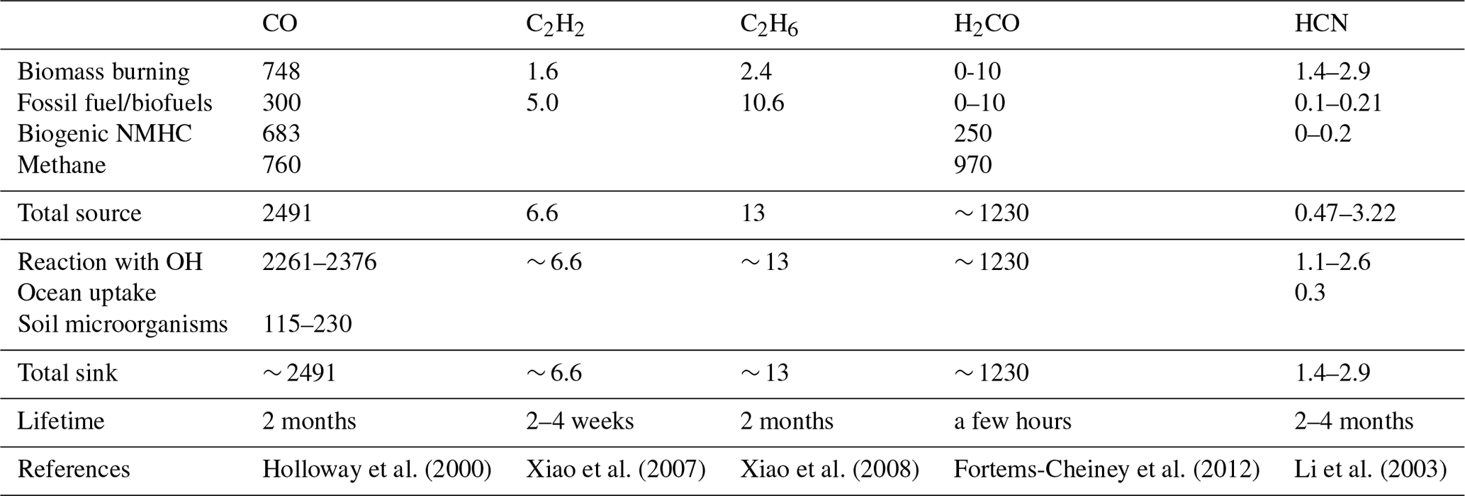
Carbon monoxide (CO) is an important atmospheric trace gas, which affects air quality and the radiative balance of the Earth (IPCC, 2013). CO reacts with hydroxyl radicals (OH) and changes the atmospheric oxidizing capacity. CO is also a good trace gas to study long-distance transport of fire and biomass burning emissions (Duflot et al., 2010; Zhou et al., 2018), as it has a relatively long lifetime of about 2 months (Khalil and Rasmussen, 1990). Atmospheric CO is mainly emitted from biomass burning, fossil fuel combustion, and oxidation from methane (CH₄) and other biogenic non-methane hydrocarbons (NMHCs) and is removed mainly by the reaction with OH and partly by uptake by soil microorganisms (Holloway et al., 2000). Ethane (C₂H₆) and acetylene (C₂H₂) are two major NMHCs. The sources of C₂H₂ and C₂H₆ are combustions from fossil fuel, biofuels, and biomass burning, and the sink of C₂H₂ and C₂H₆ is the reaction with OH (Xiao et al., 2007, 2008). C₂H₆ is a strong source of peroxyacetyl nitrate (PAN), a reservoir for nitrogen dioxide (NO₂). NO₂ normally has a short lifetime, but in the form of PAN it can be transported over long distances to a remote place, leading to an important impact on the tropospheric ozone formation. The C₂H₂ oxidation by OH can form secondary organic aerosols, affecting the atmospheric chemistry (Volkamer et al., 2009). C₂H₆ has a similar lifetime to CO of about 2 months (Rudolph, 1995). C₂H₂ has a relatively short lifetime of 2 to 4 weeks (Xiao et al., 2007). Hydrogen cyanide (HCN) is a colorless and highly poisonous gas that is less reactive than CO and has a lifetime of 2–4 months. Atmospheric HCN's main sources are biomass burning, biogenic emissions, and biofuels combustion, and it is mainly removed by the reaction with OH and ocean uptake (Li et al., 2000, 2003). Formaldehyde (H₂CO) is another important trace gas, mainly produced by methane and NMHCs oxidation in the atmosphere (Fortems-Cheiney et al., 2012). H₂CO in the atmosphere reacts quickly with OH, NO₃, Cl, and Br, leading to a typical lifetime of a few hours (Anderson et al., 2017). H₂CO is a major intermediate product in the degradation of isoprene in the atmosphere, and it strongly affects the tropospheric ozone formation (Finlayson-Pitts and Pitts, 1993). The main sources and sinks of global CO, C₂H₂, C₂H₆, H₂CO, and HCN are summarized in Table 1.

Holloway et al. (2000)Xiao et al. (2007)Xiao et al. (2008)Fortems-Cheiney et al. (2012)Li et al. (2003)

Table 1 Global sources and sinks of atmospheric CO, C₂H₂, C₂H₆, H₂CO, and HCN (Tg yr⁻¹). Blank spaces indicate when the source or sink from that component is negligible.

Because of the common sources and sinks (Table 1), a number of studies have used the ratio of C₂H₂ to CO as a tracer of the age of air to investigate the relative importance of dilution and chemistry (Xiao et al., 2007; Parker et al., 2011). In addition, the emission factors of biomass burning or forest fire were calculated and evaluated based on available aircraft observations (Goode et al., 2000; Xiao et al., 2007; Wetzel et al., 2021) and ground-based measurements (Zhao et al., 2002; Vigouroux et al., 2012; Lutsch et al., 2016). However, the variations and correlations of CO, C₂H₂, C₂H₆, H₂CO, and HCN in polluted area in northern China are not well known due to limited measurements. It is expected that these species are strongly affected by the anthropogenic emission there, but can we also capture the fire emissions?

In June 2018, we started measuring mid-infrared high spectral resolution solar absorption spectra using a new ground-based Fourier transform infrared (FTIR) spectrometer (Bruker IFS 125HR) at Xianghe (39.75^∘ N, 116.96^∘ E; 36 m a.s.l.), China. Such FTIR measurements are compliant with the Network for Detection of Atmospheric Composition Change – InfraRed Working Group (NDACC-IRWG) (De Mazière et al., 2018) protocols. In contrast to most NDACC FTIR sites, which are located in remote areas, the Xianghe site is located in a highly populated area with strong anthropogenic emissions from fossil fuel and biofuels combustion among other sources (Yang et al., 2020; Zhou et al., 2021). In this study, we present the first time series of FTIR retrievals of CO, C₂H₂, C₂H₆, H₂CO, and HCN at Xianghe, covering 3 years of measurements, and their use to investigate the variations in CO, C₂H₂, C₂H₆, H₂CO, and HCN columns on both seasonal and synoptic scales, as well as their correlations. Moreover, the FTIR measurements, atmospheric model, and satellite measurements are used to understand the sources of CO, C₂H₂, C₂H₆, H₂CO, and HCN columns in this region. Section 2 gives a brief introduction to the FTIR instrument and discusses the retrieval strategies, retrieval information, and uncertainties. The time series, variations, and correlations of CO, C₂H₂, C₂H₆, H₂CO, and HCN total columns are analyzed in Sect. 3. the FLEXible PARTicle dispersion (FLEXPART) model is used to understand the sources of the observed air masses at Xianghe. The VIIRS satellite observations are applied to locate the fire emission in the boreal forest. Based on the CO anthropogenic emissions and the ratios of C₂H₂ and C₂H₆ to CO derived from the FTIR measurements, we derive the C₂H₂ and C₂H₆ emissions in northern China and compare them to the inventories. Finally, the conclusions are drawn in Sect. 4.

2 FTIR measurements

2.1 Instrument

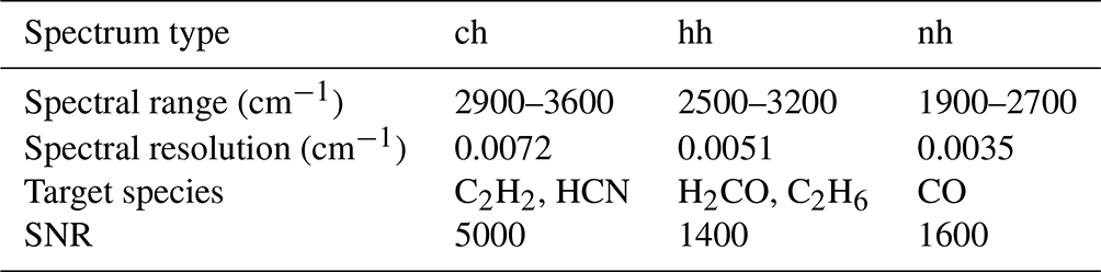
A Bruker IFS 125HR spectrometer was installed at Xianghe in 2016 and started recording solar absorption spectra in June 2018 (Zhou et al., 2020, 2021). The mid-infrared spectra covering the spectral range from 1800 to 5500 cm⁻¹ are recorded with an Indium antimonide (InSb) detector, cooled with liquid nitrogen. To increase the signal-to-noise ratio (SNR) of the spectrum used for specific target species, 6 NDACC-IRWG recommended optical filters (Blumenstock et al., 2021) are mounted in the wheel in front of the detector. Figure 1 shows three types of spectra (ch, hh, and nh) used in this study, and the main characters of these spectra are listed in Table 2.

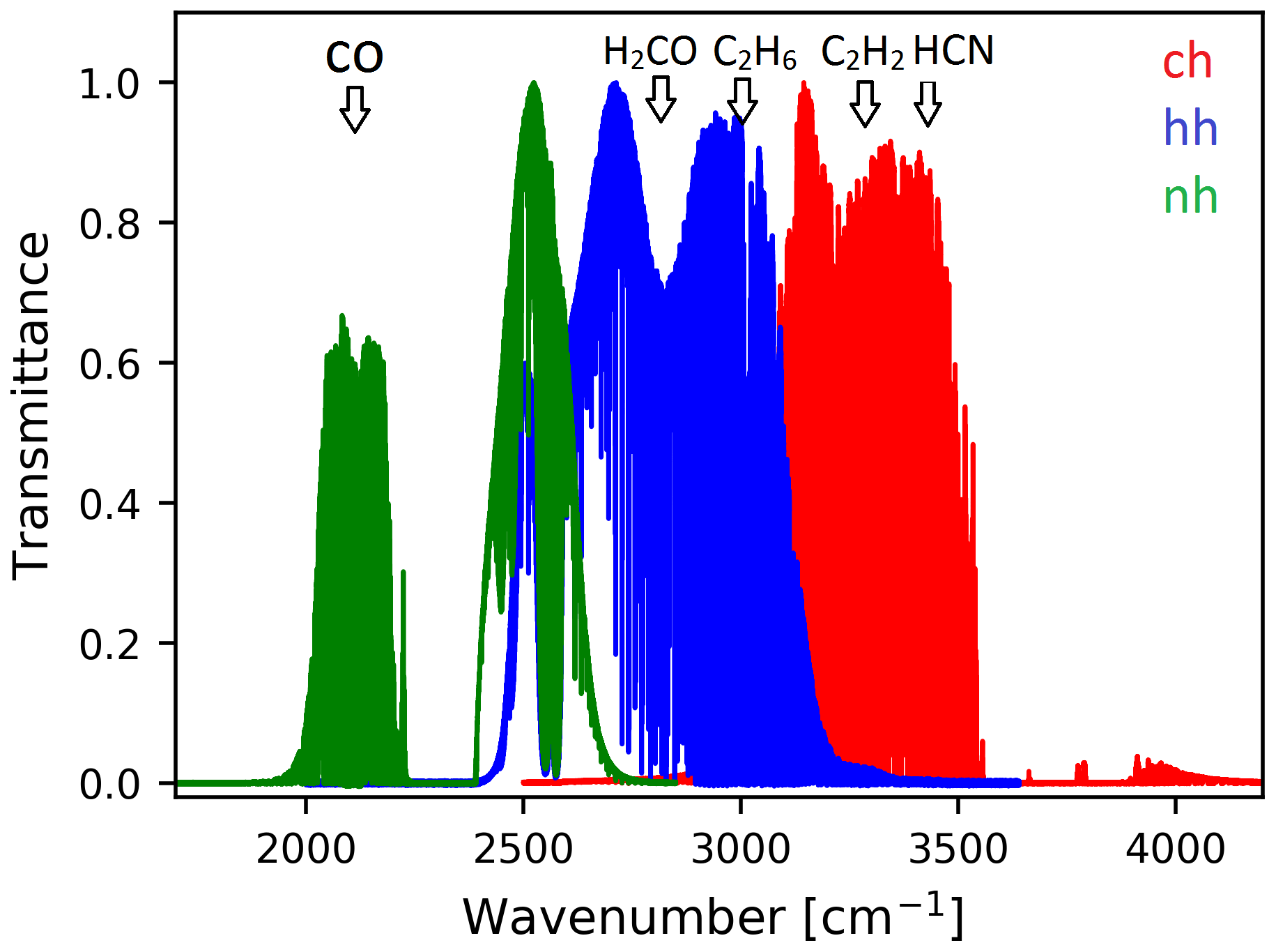
Figure 1 Normalized spectra (ch, hh, and nh) with three different filters used for CO, C₂H₂, C₂H₆, H₂CO, and HCN retrievals at Xianghe.

Table 2 The characters of the three types of spectra observed at Xianghe used to retrieve CO, C₂H₂, C₂H₆, H₂CO, and HCN.

To understand the optical status of the FTIR instrument, HBr cell spectra were recorded on 7 June 2018, 9 September 2018, 18 July 2019, 20 December 2019, and 13 September 2021. The instrument line shape (ILS) parameters, modulation efficiency (ME) and phase error (PE), are retrieved by the LINEFIT14.5 algorithm (Hase et al., 1999). Figure 2 shows that the ME is relatively stable, with about 0.86 at the maximum optical path difference (250 cm), and that the PE is more variable with time. To reduce the retrieval uncertainty from the ILS, the LINEFIT outputs are used to represent the real ILS in the retrieval algorithm.

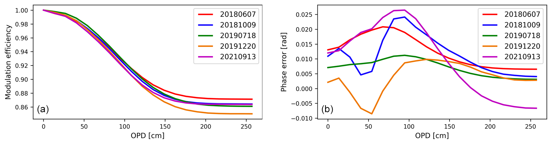
Figure 2 The retrieved modulation efficiency (a) and phase error (b) from the HBr cell measurements on 7 June 2018, 9 September 2018, 18 July 2019, and 13 September 2021 by the LINEFIT14.5 algorithm.

2.2 Retrieval strategies

The SFIT4 retrieval code (version 1.0.18), updated from SFIT2 (Pougatchev et al., 1995), is applied to retrieve CO, C₂H₂, C₂H₆, H₂CO, and HCN profiles from the FTIR spectra at Xianghe. The SFIT4 code is well established and widely used in the NDACC-IRWG. The retrieval algorithm includes a line-by-line model F(x,b) with the state vector x (retrieved parameters) and non-retrieved parameters b inputs to calculate the transmittance Y at a given spectral range:

$$\begin{array}{}\text{(1)}& \mathit{Y}=\mathit{F}(\mathit{x},\mathit{b})+\mathit{ϵ},\end{array}$$

where ϵ denotes the error. There are 47 layers between the surface and the top of the atmosphere (100 km) included in the forward model. The retrieval windows for these species are listed in Table 3, and the absorption lines within each window are shown in Fig. 3. The retrieval windows are followed the NDACC-IRWG recommendation and several previous FTIR studies (Zhao et al., 2002; Vigouroux et al., 2012; Viatte et al., 2014; Zhou et al., 2018; Vigouroux et al., 2018). Interfering species are retrieved along with the target species to reduce their impacts. The important interfering species are performed as a profile retrieval due to their strong absorption lines, and the other species are performed as a column retrieval (see Table 3). The atmospheric line list (ATM20), provided by Geoff Toon (JPL, NASA), is used for the CO, C₂H₂, and HCN retrievals, the ATM18 is used for the H₂CO retrieval, and the pseudo line list, also provided by Geoff Toon (https://mark4sun.jpl.nasa.gov/pseudo.html; last access: 15 April 2022), based on the cross section made by Harrison et al. (2010), is used to retrieve C₂H₆. Note that the current NDACC-IRWG retrieval strategies for CO, C₂H₂, and HCN still use HITRAN08 spectroscopy (Rothman et al., 2009). We have tested both HITRAN08 and ATM20 for these three targets and their interfering species, and it is found that the fitting using ATM20 is improved, especially for CO, HCN, and H₂O (interfering). Therefore, we recommend the ATM20 for these species. As mentioned above, to minimize the impact of the instrument, the LINEFIT results are used for the ILS inputs to represent the real instrument status. In addition, wavenumber shift, phase, and slope are included in the state vector for all five species. The solar intensity and solar shift are also retrieved for CO, H₂CO and HCN because of relatively strong solar lines existed in their retrieval windows (see Fig. 3). The vertical profiles of the temperature and water vapor are interpolated to the measurement time from the National Centers for Environmental Prediction (NCEP) 6-hourly reanalysis data. Regarding H₂CO, we apply the harmonized retrieval strategy established by Vigouroux et al. (2018) for the NDACC-IRWG FTIR sites, where the average of the Whole Atmosphere Community Climate Model (WACCM) v6 monthly means between 1980 and 2020 is applied for the a priori profile. Regarding the other four species, the average of the WACCM v7 monthly means between 1980 and 2040 are applied for the a priori profiles of the target species and other interfering species, except for H₂O, HDO, H${}_{\mathrm{2}}^{\mathrm{17}}$O, and H${}_{\mathrm{2}}^{\mathrm{18}}$O, where we use NCEP reanalysis to set the a priori profiles of H₂O and its isotopes.

Table 3 The retrieval window, interfering species, spectroscopy, and fitting parameters for these five species. Note that the isotopes of H₂O (HDO, H${}_{\mathrm{2}}^{\mathrm{17}}$O, and H${}_{\mathrm{2}}^{\mathrm{18}}$O) are treated as independent species in our retrieval.

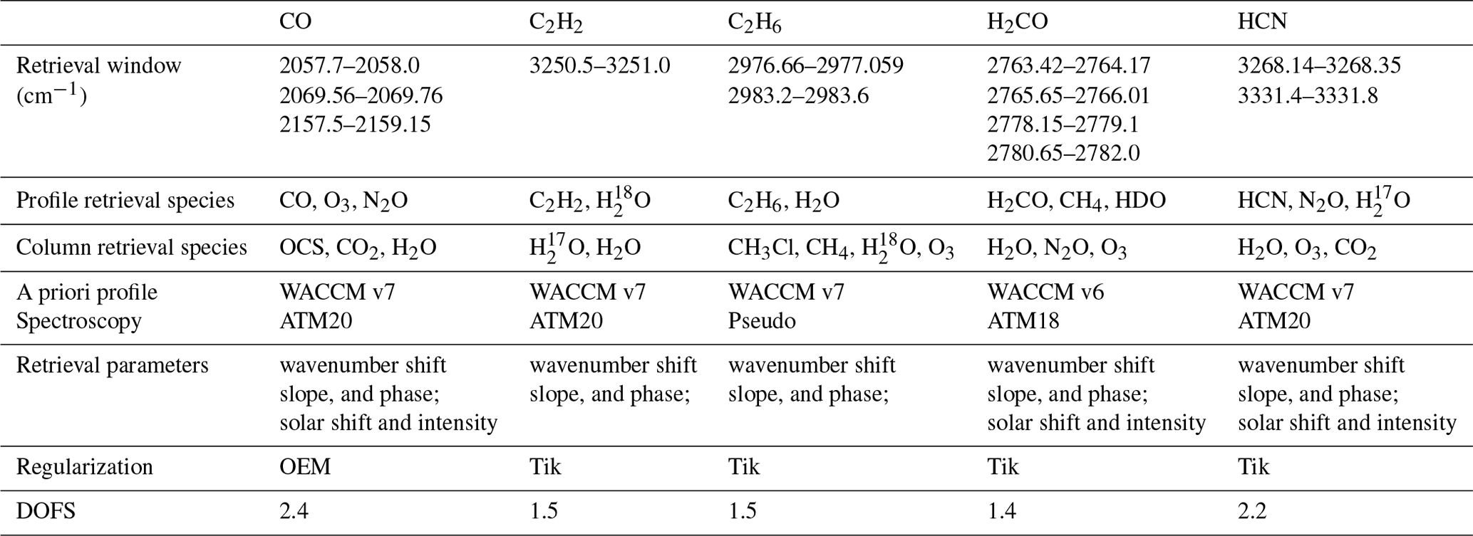
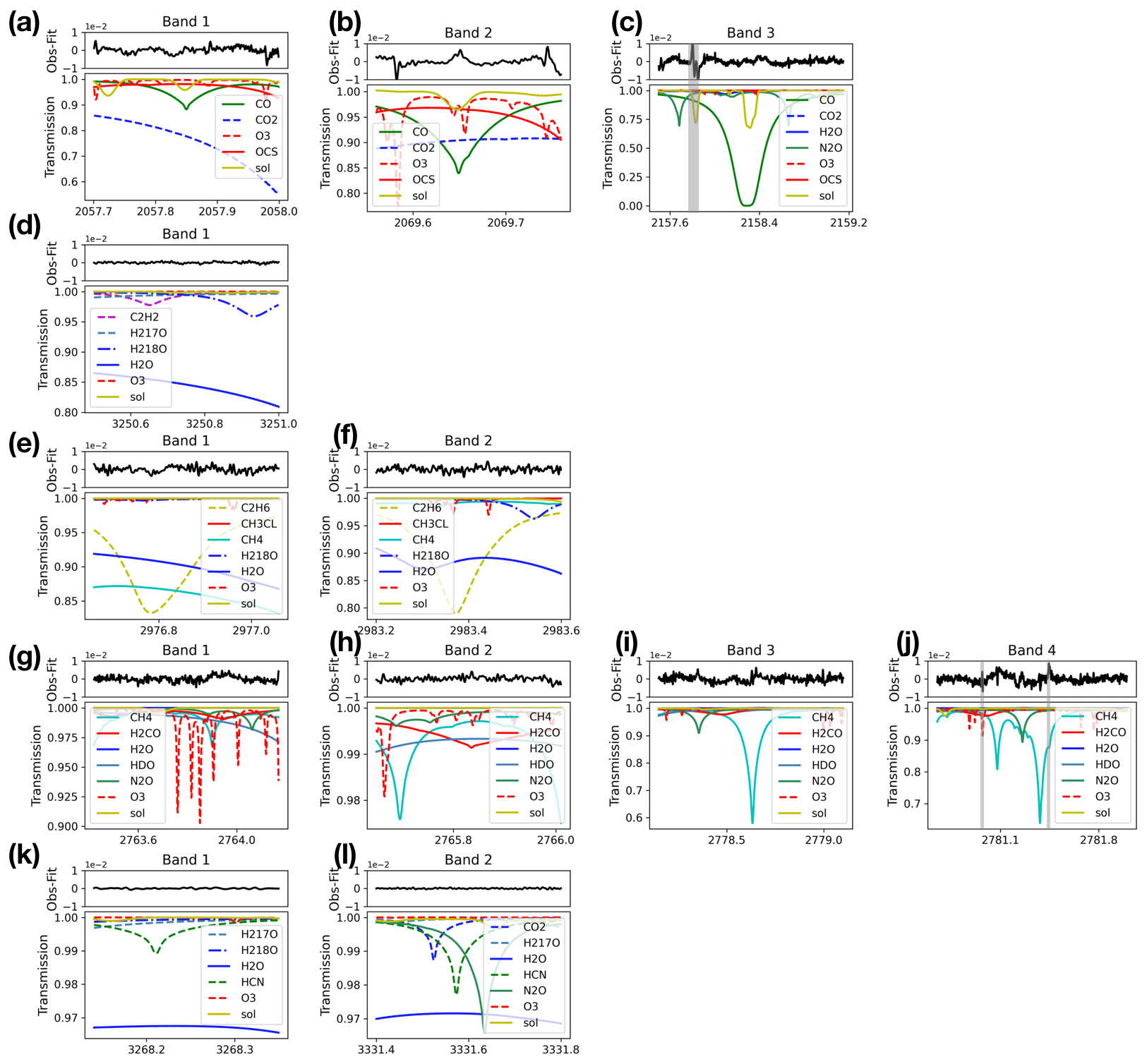
Figure 3 The retrieval windows for CO (a, b, c), C₂H₂ (d), C₂H₆ (e, f), H₂CO (g, h, i, j) and HCN (k, l). For each window, the bottom panel is the normalized transmittance from atmospheric species and the solar line, which the upper panel is the residual between the fitted and observed spectra. Note that there is one de-weighting window (2157.775–2157.905 cm⁻¹) in CO band 3 and two de-weighting windows (2780.967–2780.993; 2781.42–2781.48 cm⁻¹) in H₂CO band 4, where we set the SNR as zero due to bad fittings.

To solve this ill-posed problem (Eq. 1) and to look for the optimal x to make the simulated spectrum F(x,b) close to the measured absorption spectrum Y, a cost function J(x) is set up as follows:

$$\begin{array}{}\text{(2)}& \begin{array}{rl}\mathit{J}\mathbf{\left(}\mathit{x}\mathbf{\right)}& =[\mathit{y}-\mathit{F}\mathbf{(}\mathit{x}\mathbf{\left)}{]}^T{\mathbf{S}}_{\mathit{ϵ}}^{-\mathrm{1}}\right[\mathit{y}-\mathit{F}\mathbf{\left(}\mathit{x}\mathbf{\right)}]\\ & +[\mathit{x}-{\mathit{x}}_{\mathrm{a}}{]}^T{\mathbf{S}}_{\mathrm{R}}[\mathit{x}-{\mathit{x}}_{\mathrm{a}}].\end{array}\end{array}$$

The cost function is determined from the measurement's error covariance S_ϵ, the a priori state x_a and a regularization matrix S_R. The SNR is applied to calculate the measurement covariance S_ϵ, with the diagonal values equal to $\mathrm{1}/{\mathrm{SNR}}^{\mathrm{2}}$ and non-diagonal values equal to zero. Regarding the regularization matrix ${\mathbf{S}}_{\mathrm{R}}={\mathbf{S}}_{\mathrm{a}}^{-\mathrm{1}}$, we use the optimal estimation method (OEM) and derive the covariance matrix from the WACCM monthly means as S_a for CO. For the other four species, we use the Tikhonov L₁ method (${\mathbf{S}}_{\mathrm{R}}=\mathit{\alpha }{\mathbf{L}}_{\mathrm{1}}^T{\mathbf{L}}_{\mathrm{1}}$). To determine the value of α, we first use the WACCM monthly means to generate a covariance matrix, apply the retrieval using OEM, and then apply the retrieval using the Tikhonov method by tuning the α values to make the degree of freedom for the signal (DOFS) close to the OEM results (Steck, 2002). As a result, α values are set as 10, 100, 100, and 30 for C₂H₂, C₂H₆, H₂CO, and HCN, respectively. After that, the retrieved state vector x_r can be calculated with the Levenberg–Marquardt iteration algorithm. Note that the OEM or Tikhonov regularization is selected based on the a priori knowledge. For CO, we have surface in situ measurements at Xianghe, which agree well with WACCM model simulations. The reason is probably that there are many surface in situ and aircraft profile measurements around the world (e.g., NOAA networks, HIPPO campaign). As the WACCM CO simulations perform well at Xianghe, we use the OEM method for CO, and the a priori covariation matrix is derived from the WACCM model. However, for the remaining four species, we have no surface measurement at Xianghe and it is hard to evaluate the performance of the WACCM model simulations. Therefore, we apply the Tikhonov L1 method for these targets so that the retrievals are less affected by the a priori profiles.

2.3 Retrieval information

According to the optimal estimation method (Rodgers, 2000), the retrieved parameters can be written as

$$\begin{array}{}\text{(3)}& {\mathit{x}}_{\mathrm{r}}={\mathit{x}}_{\mathrm{a}}+\mathbf{A}\left({\mathit{x}}_{\mathrm{t}}-{\mathit{x}}_{\mathrm{a}}\right)+\mathit{ϵ},\end{array}$$

where x_r, x_a, and x_t are the retrieved, a priori, and true state vector, respectively; A is the averaging kernel (AVK), representing the sensitivity of the retrieved parameters to the true statuses; and ϵ is the retrieval uncertainty, which will be discussed in Sect. 2.4. The a priori and retrieved profiles, together with the averaging kernels, are shown in Fig. 4. For all these species, the retrieved profiles are mainly sensitive to the troposphere and lower stratosphere. There is a discontinuity found in the AVK of C₂H₂ and C₂H₆ because the mole fractions of C₂H₂ and C₂H₆ a priori profile (WACCM) become very low above 20 and 22 km, respectively. The pressure and temperature dependences of the absorption lines allow us to get some vertical information, but the vertical resolution is limited. The trace of the averaging kernel is the DOFS, indicating the number of independent pieces of the information. The DOFS for these species are listed in Table 3. The DOFS of C₂H₂, C₂H₆, and H₂CO are close to 1.5, and the DOFS of CO and HCN are close to 2.3, which indicates that we can derive two partial columns for CO and HCN at Xianghe. Based on the retrieved profile, we can obtain the total column (C_r)​​​​​​​:

$$\begin{array}{}\text{(4)}& C_{\mathrm{r}}={\mathbf{PC}}_{\mathrm{air}}\cdot {\mathit{x}}_{\mathrm{r}}={\mathbf{TC}}_{\mathrm{a}}+{\mathbf{A}}_{\mathrm{c}}\cdot \left({\mathbf{PC}}_{\mathrm{t}}-{\mathbf{PC}}_{\mathrm{a}}\right)+{\mathit{ϵ}}_{\mathrm{c}},\end{array}$$

where PC_air is the dry air partial column profile, PC_a and PC_t are the a priori and true partial columns of the target species, A_c is the column averaging kernel, representing the sensitivity of the retrieved total column to the true partial column profiles, and ϵ_c is the retrieval uncertainty of the total column. If A_c=1 at one layer, the C_r can capture the deviation of the partial column well from the a priori partial column (PC_t−PC_a) in that layer. If A_c<1 at one layer, the C_r underestimates the deviation of the partial column from the a priori partial column in that layer and vice versa.

Figure 4 The upper row shows the a priori profiles (black) and retrieved profiles (solid red line: mean; dashed red area: standard deviation) for CO, C₂H₂, C₂H₆, H₂CO, and HCN. The lower row shows the averaging kernels and the column averaging kernels (divided by 10) for these species.

The a priori profiles and retrieved profiles (Fig. 4) show that the mole fractions in the lower troposphere are larger than those at higher altitudes for all of these species. Note that the CO mole fraction in the mesosphere is even larger than that in the lower troposphere due to the photolysis of carbon dioxide (Garcia et al., 2014), but it accounts for less than 1.0 % of the total column. Based on the mean retrieved profile, the partial column between surface and 10 km accounts for 91.4 %, 97.6 %, 95.2 %, 97.9 %, and 80.1 % in the total column of CO, C₂H₂, C₂H₆, H₂CO, and HCN, respectively. The retrieved CO total column has good sensitivity to the lower troposphere and stratosphere. The retrieved C₂H₂ and C₂H₆ total columns are mainly sensitive to the vertical range between the surface and 20 km, but they underestimate the deviation from the a priori partial column in the lower troposphere and overestimate the deviation from the a priori partial column in the upper troposphere and stratosphere. The retrieved H₂CO total column has good sensitivity in the lower stratosphere, but overestimates the deviation from the a priori partial column above. The retrieved HCN total column is sensitive to the vertical range between the surface to about 40 km, where it underestimates the deviation from the a priori partial column in the lower troposphere and upper stratosphere but overestimates the deviation from the a priori partial column in the upper troposphere and the lower stratosphere.

2.4 Retrieval uncertainty

The retrieval uncertainty on profile can be expanded as (Rodgers, 2000) follows:

$$\begin{array}{}\text{(5)}& {\mathit{ϵ}}_{\mathrm{r}}=\left(\mathbf{A}-\mathbf{I}\right)\left({\mathit{x}}_{\mathrm{t}}-{\mathit{x}}_{\mathrm{a}}\right)+{\mathbf{GK}}_b\left({\mathit{b}}_{\mathrm{t}}-\mathit{b}\right)+\mathbf{G}{\mathit{ϵ}}_y,\end{array}$$

where A is the averaging kernel of the state vector; x_t and x_a are the true and a priori state vector, respectively; G is the contribution function; b_t and b are the true and used model parameters, which affect the forward model but are not included in the state vector, such as spectroscopy, temperature, solar zenith angle (SZA), and zero offset (zshift); ${\mathbf{K}}_b=\frac{\partial \mathit{F}(\mathit{x},\mathit{b})}{\partial \mathit{b}}$ is the weighting function of the model parameters, representing the sensitivity of the parameter b to the forward model (F(x,b)); and ϵ_y is the measurement noise.

The covariance of the retrieval uncertainty S_r can be written as follows:

$$\begin{array}{}\text{(6)}& {\mathbf{S}}_{\mathrm{r}}=(\mathbf{A}-\mathbf{I}){\mathbf{S}}_{\mathit{a}}(\mathbf{A}-\mathbf{I}{)}^T+{\mathbf{GK}}_b{\mathbf{S}}_{\mathit{b}}{\mathbf{K}}_b^T{\mathbf{G}}^T+{\mathbf{GS}}_{{\mathit{ϵ}}_y}{\mathbf{G}}^T.\end{array}$$

Table 4 The systematic and random (sys/ran) retrieval uncertainties for the total columns of five target species. The “–” means that the uncertainty is less than 0.1 %. The SD of each species within ±1 h around local noon are shown in the bottom row to represent the variability of the retrieval.

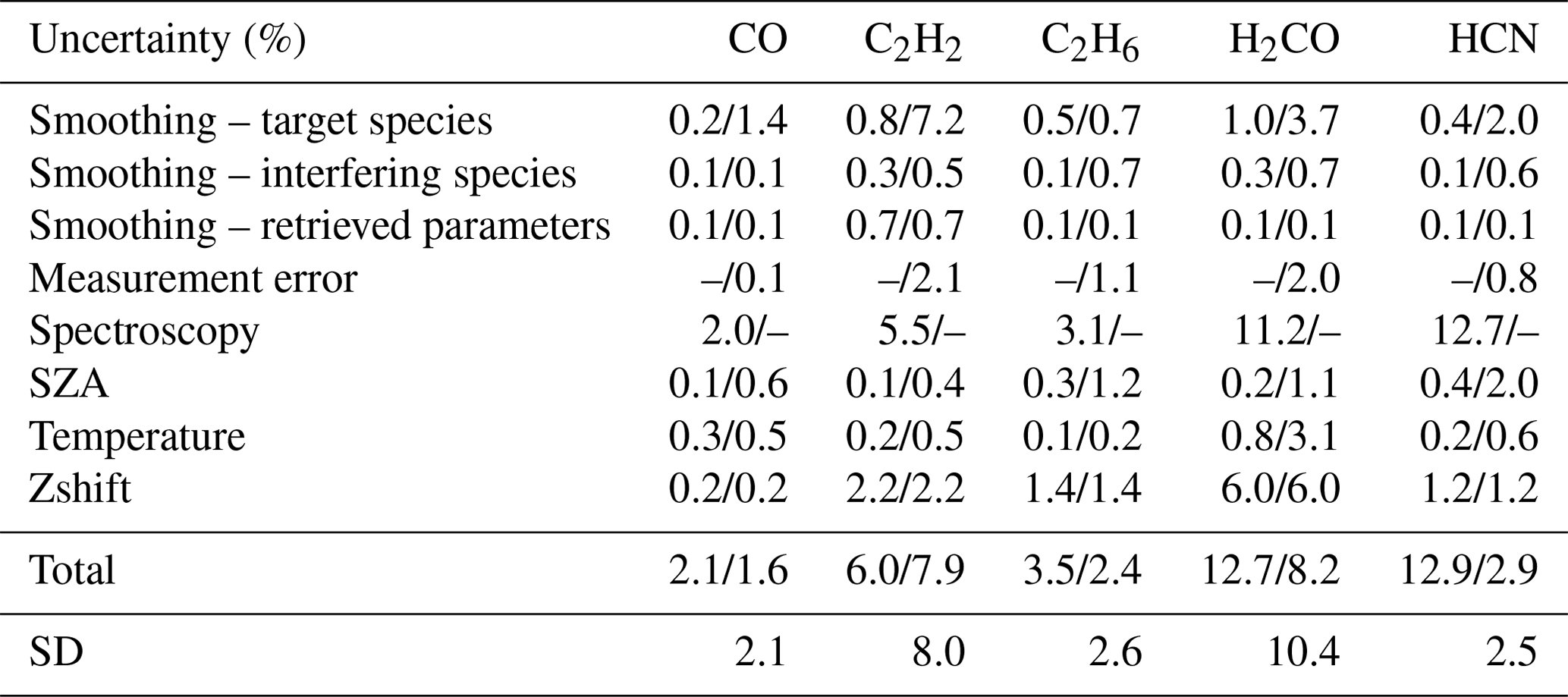
On the right side of Eq. (6), the three items are the smoothing error, the model parameter error, and the measurement noise error, respectively. Here, we assume the forward model error is negligible. Note that the state vector (x) contains not only the profile of the target species but also the interfering species and other retrieved parameters (see Table 3). Therefore, we separate $(\mathbf{A}-\mathbf{I})({\mathit{x}}_{\mathrm{t}}-{\mathit{x}}_{\mathrm{a}})$ into three parts (Zhou et al., 2016): the smoothing error from the target gas uncertainty, the interfering species uncertainty, and other retrieved parameter uncertainties (slope, wavenumber shift, etc.). For the model parameter error, we list the important parameters (spectroscopy, SZA, temperature and zshift) in Table 4. The SNR is applied to calculate the measurement noise (${\mathit{ϵ}}_y=\mathrm{1}/\mathrm{SNR}$). It is assumed that the measurement noise is purely random uncertainty. We need to set the uncertainties for other components based on a priori knowledge or other datasets because x_t and b_t are not known. For the smoothing error estimation, we set 20 % as the systematic uncertainty, and the random uncertainties are derived from the variations in WACCM model monthly means between 1980 and 2040. For the temperature profile, the systematic and random uncertainties are calculated from the mean and standard deviation (SD) of the differences between the NCEP and the European Centre for Medium-Range Weather Forecasts (ECMWF) ERA5 reanalysis data at Xianghe in the time period of 2016–2019. In general, the systematic uncertainty is about 1.0 K in the whole atmosphere and random uncertainty is about 2 K in the lower troposphere and about 1 K above. We estimate 0.1 % and 0.5 % for the systematic and random uncertainties of SZA, 1.0 % for both systematic and random uncertainties of zshift. The uncertainty of the spectroscopy is set as 2.0  %, 5.0 %, 10.0 %, and 10.0 % for CO, C₂H₂, H₂CO, and HCN, respectively, based on the HITRAN2016 (Gordon et al., 2017). The uncertainty of the spectroscopy of C₂H₆ is set as 3 %, according to the pseudo line list (https://mark4sun.jpl.nasa.gov/pseudo.html). The total retrieval uncertainties of these species are also shown in Table 4. The systematic uncertainty is mainly from the spectroscopy, while the random uncertainty is mainly from smoothing error, SZA, temperature, and zshift. The mean of the SD of all measurements within ±1 h around local noon (with at least two measurements) is calculated to represent the variability of the retrieval. In general, the SDs are close to the estimated random uncertainties for all species.

3 Results and discussion

3.1 Time series and seasonality

The time series of the FTIR CO, C₂H₂, C₂H₆, H₂CO, and HCN total columns at Xianghe between June 2018 and November 2021 are shown in Fig. 5. Due to the COVID-19 lockdown, liquid nitrogen could not be delivered to the site. Therefore, there is a 3-month gap between 18 February and 23 May 2020. To better visualize the seasonal variation, the total columns are fitted by a periodic function y(t):

$$\begin{array}{}\text{(7)}& y\left(t\right)=A_{\mathrm{0}}+\sum _{k=\mathrm{1}}^{\mathrm{3}}\left(A_{\mathrm{2}k-\mathrm{1}}\cos \left(\mathrm{2}k\mathit{\pi }t\right)+A_{\mathrm{2}k}\sin \left(\mathrm{2}k\mathit{\pi }t\right)\right)+\mathit{ϵ},\end{array}$$

where A₀ is the offset and A₁ to A₆ are the periodic amplitudes, representing the seasonal variation; ϵ is the uncertainty.

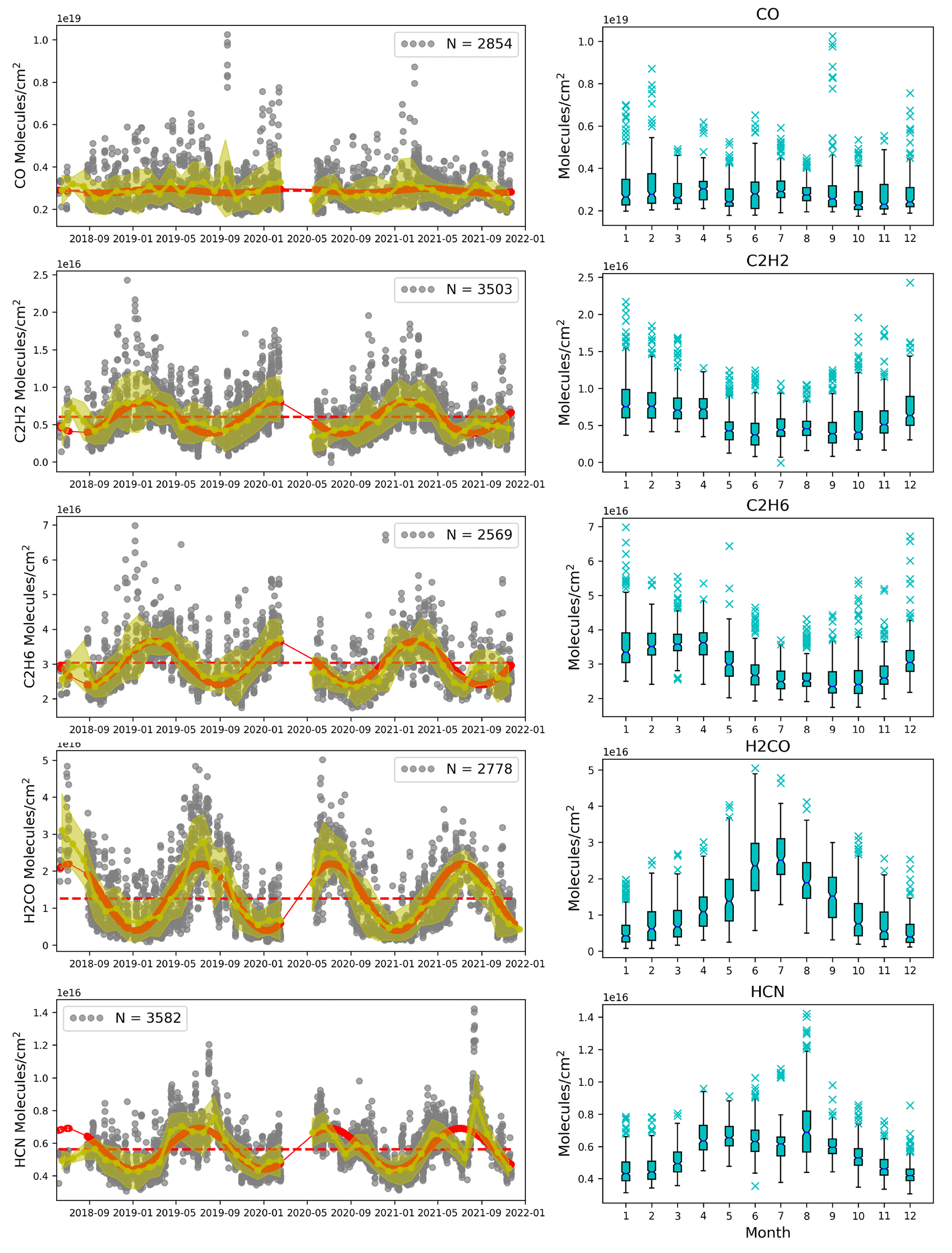
Figure 5 The left column shows the time series of CO, C₂H₂, C₂H₆, H₂CO, and HCN FTIR retrieved total columns between June 2018 and November 2021 at Xianghe. Gray dots are each individual retrievals with the total number indicated by N, the dotted yellow line is the monthly mean together with the yellow shaded area as the monthly standard deviation, the dashed red line is the offset A₀, and the solid red line is the fitted time series y(t). The right column shows the monthly box plot of the total columns. The bottom and upper boundaries of the box represent the 25 % (Q1) and 75 % (Q3) percentile of the data points around the median value, the error bars extend no more than 1.5 times the interquartile range (IQR = Q3 − Q1) from the edges of the box, and the blue crosses are the extremely high values.​​​​​​​

3.1.1 CO

The mean and SD of CO total column are 2.86 ± 0.87 × 10¹⁸ molec. cm⁻². There is no clear seasonal variation, with a peak-to-peak amplitude of seasonal variation of less than 5 %. A similar seasonal variation in CO total column is observed by the TROPOspheric Monitoring Instrument (TROPOMI) onboard the S5P satellite measurements and Total Carbon Column Observing Network (TCCON) measurements at Xianghe (Appendix A).

CO in the atmosphere is mainly emitted from biomass burning and biogenic and anthropogenic emissions and removed by reaction with OH (Duncan et al., 2007). Significant seasonal variations in CO columns are observed at other FTIR sites (Zeng et al., 2012; Viatte et al., 2014; Té et al., 2016; Sun et al., 2020). For example, high values in spring and low values in autumn are observed by FTIR measurements in Paris, a megacity in western Europe. Té et al. (2016) used the GEOS-Chem model to understand the seasonal variation in CO columns in Paris, and they found that the dominant factor is the anthropogenic emission and that more emissions are observed in spring. According to the anthropogenic emission datasets, such as the Regional Emission inventory in ASia (REAS) v3.2 (Kurokawa and Ohara, 2020) and the Emissions Database for Global Atmospheric Research (EDGAR) v5.0 (Crippa et al., 2018), the CO emissions in northern China are high in winter and low in summer, with a relative difference of about 30 %. Regarding the sink, more UV intensity in summer in northern China (Hu et al., 2010) can generate a high OH level (Canty and Minschwaner, 2002). As a result, more OH in summer as compared to winter could also lead to a high CO column in winter. However, such a phase of the seasonal variation is hardly observed by the FTIR total columns. One possible reason is that the CH₄ mole faction is high in summer in northern China, which is very different from other sites with a similar latitude (Karlsruhe, Germany, and Lamont, USA) (Yang et al., 2020). CH₄ is also an important source of CO, and a high CH₄ level in summer at Xianghe will probably compensate for the impact of the lower anthropogenic CO emission and the stronger OH sink in summer. Another possible reason is that the Xianghe site is very close to the anthropogenic sources, so the seasonal variation in OH has a weak effect on CO. To conclude, the small month-to-month variation in CO columns observed at Xianghe shows that the synoptic variation in CO columns is much stronger than the seasonal variation in northern China.

3.1.2 C₂H₂ and C₂H₆

C₂H₂ and C₂H₆ belong to the non-methane hydrocarbons (NMHCs) category. The mean and SD of C₂H₂ and C₂H₆ total columns are 0.60 ± 0.29 × 10¹⁶ and 3.02 ± 0.70 × 10¹⁶ molec. cm⁻², respectively. There is a clear seasonal variation in both species, with a high value in January–April and a low value in June–September. The peak-to-peak amplitudes of the fitted seasonal variations are 0.38 × 10¹⁶ and 1.16 × 10¹⁶ molec. cm⁻² for C₂H₂ and C₂H₆, respectively, corresponding to 62 % and 38 % of their mean values. The major sources of C₂H₂ and C₂H₆ are biofuels and fossil fuel, and the main sink is the reaction with OH. A slightly larger seasonal variation found in C₂H₂ as compared to C₂H₆ is consistent with the fact that C₂H₂ is removed more quickly by OH as compared to C₂H₆ (Xiao et al., 2007, 2008). According to the REAS v3.2 inventory, more C₂H₂ and C₂H₆ are emitted in winter as compared to summer, and the relative difference can reach 100 %. The seasonal variations in C₂H₂ and C₂H₆ at Xianghe are in agreement with the measurements at two Japanese sites (Moshiri and Rikubetsu) (Zhao et al., 2002).

3.1.3 H₂CO and HCN

The mean and SD of H₂CO and HCN total column are 1.26 ± 0.91 × 10¹⁶ and 0.57 ± 0.14 × 10¹⁶ molec. cm⁻², respectively. In contrast to the seasonal variation in C₂H₂ and C₂H₆, the seasonal variations in H₂CO and HCN show a high value in summer and low value in winter. H₂CO is mainly formed by the oxidation from methane and other hydrocarbons, which are emitted into the atmosphere by plants, animals, human activities, and biomass burning. Shen et al. (2019) used the GEOS-Chem model to quantify the H₂CO contributions in China, and they pointed out that H₂CO is mainly generated from anthropogenic and biogenic sources. Based on the FTIR measurements at Xianghe, Ji et al. (2020) found that the CH₄ tropospheric column reaches its maximum in summer, and the carbon tracker model shows that there are large natural emissions (wetlands, soil, oceans, and insects or wild animals) in summer. HCN is a good tracer of biomass burning, and its lifetime is about 2–4 months (Li et al., 2000). The seasonal variation in HCN at Xianghe is similar to those observed at Kiruna, Toronto, Rikubetsu, and Hefei (Sun et al., 2020), with two peaks around May and September. Sun et al. (2020) applied GEOS-Chem tagged CO simulation to understand that the peaks in May and September at Hefei are mainly from the biomass burning emissions at surrounding regions. FTIR measurements at Xianghe show that there is a low value of the HCN column in July 2021 followed by a high peak in August 2021, which will be further discussed in Sect. 3.4.

3.2 Correlation

According to EDGAR v5.0 and REAS v3.2 anthropogenic emission datasets, the spatial distributions of CO, C₂H₂, C₂H₆, and H₂CO are very similar, with a large emission around Xianghe in northern China. In this section, the correlations between CO and the other four species are investigated. CO is treated as a tracer gas here because the FTIR CO retrieval has the lowest random uncertainty as compared to other species (Table 4). To reduce the impact of the atmospheric background and capture the day-to-day variation, the monthly median are removed from the total column (Δgas = gas − monthly median). High correlations are found between ΔCO and the other four species with the Pearson correlation coefficients (R) of 0.80, 0.70, 0.70, and 0.68 for ΔC₂H₂, ΔC₂H₆, ΔH₂CO, and ΔHCN, respectively (Fig. 6). The intercepts of the four fitting lines are very close to zero, confirming that subtracting the monthly means can remove the atmospheric background signal well. The slope of the fitting represents the enhanced ratio of the target gas column to the CO column.

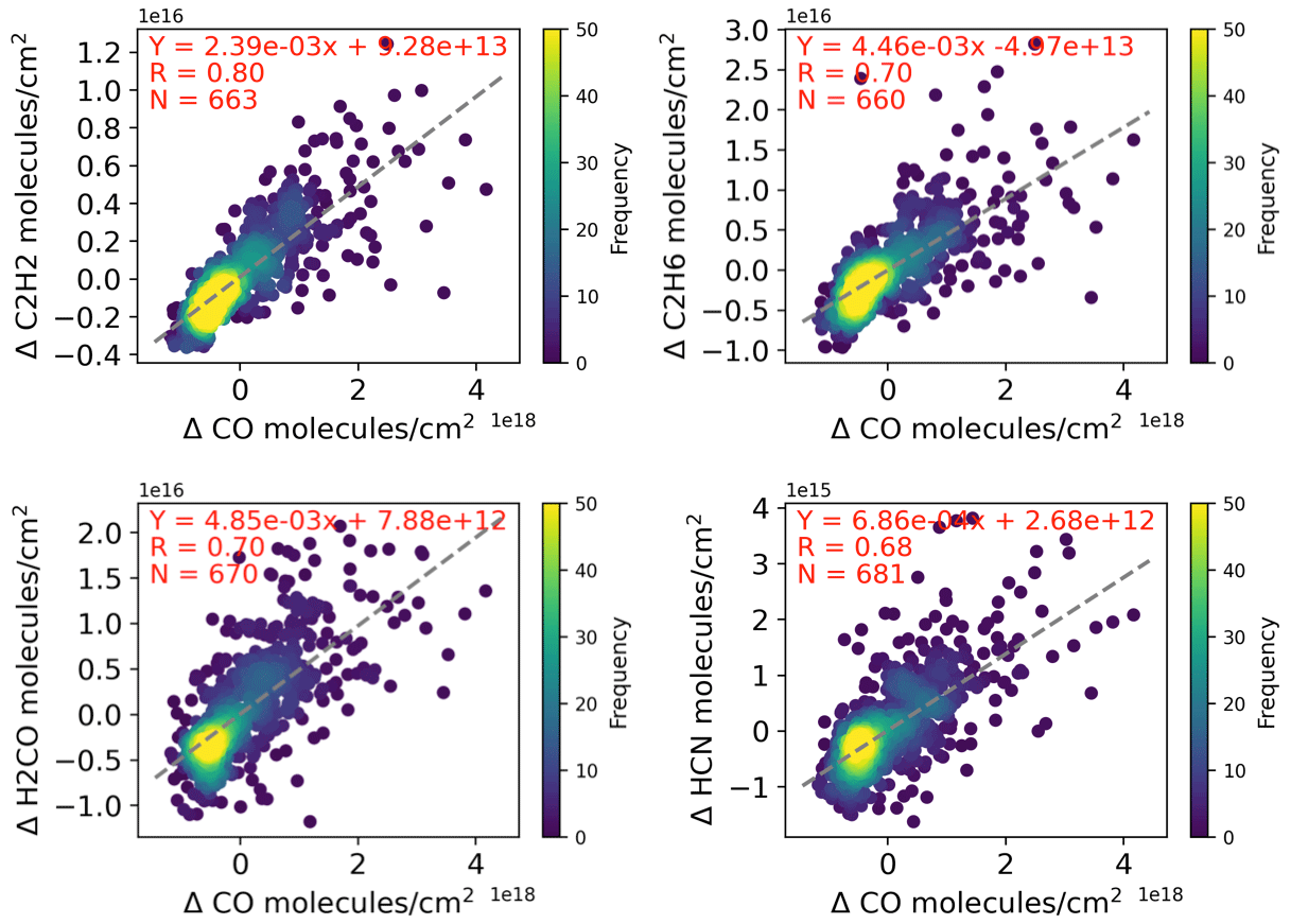
Figure 6 The correlation plot between ΔCO (CO minus monthly mean) and ΔC₂H₂, ΔC₂H₆, ΔH₂CO, and ΔHCN daily means. The dots are colored according to their frequency. The dashed gray line is the linear fit. R is the Pearson correlation coefficient. N is the co-located number.

Figure 7 Similar to Fig. 6 but for the four seasons.

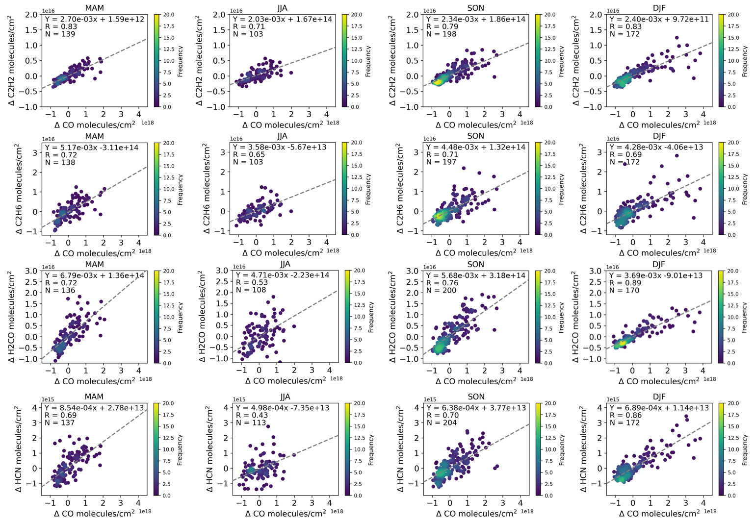
To check whether there is a seasonal dependence in their correlations, the correlation plots in four seasons are shown in Fig. 7. It is noticed that we have fewer measurements in summer because summer is the rainy season at Xianghe, and the FTIR measurements are only performed under good weather conditions. R values are relatively high in spring, autumn, and winter. Relatively low R values are found in summer for all species, which is due to the fact that there are smaller anthropogenic emissions and more oxidation production in summer (Sun et al., 2020). Regarding the fitting slope, it is found that the slopes in summer are relatively lower than those in the other three seasons for C₂H₂, C₂H₆, and HCN. The REAS v3.2 inventory provides CO, C₂H₂, and C₂H₆ monthly emissions, meaning that we can calculate the monthly ratios of the C₂H₂ and C₂H₆ emissions to the CO emission in northern China. The monthly emission ratios have a minimum in summer for both C₂H₂ and C₂H₆, which is generally in good agreement with our FTIR measurements. Different from the other three species, the lowest slope between CO and H₂CO is observed not in summer but in winter. H₂CO has a short lifetime, and the formation of H₂CO does not mainly come from the direct emissions but from the oxidation reaction.

3.3 Air mass source

In this section, the Lagrangian particle dispersion model FLEXPART v10.4 model is used to understand the air mass sources observed by the FTIR measurements at Xianghe. The backward running of the FLEXPART model releases the air particles at the Xianghe site and traces back to where the air mass comes from, providing source–receptor relationships. For more details about the FLEXPART v10.4 model, we refer readers to Pisso et al. (2019) and references therein. As the high mole fractions of these five species are located in the boundary height (see Fig. 4), we release particles in the vertical range between the surface and 2 km. In addition, as the FTIR only does measurement during the daytime, we set the releasing temporal window as ±1 h around local noon for all FTIR measurement days between 1 June 2018 and 30 November 2021. The CO molecule is used as the trace gas. The main settings of FLEXPART are listed in Table 5. The model is driven by the National Centers for Environmental Prediction (NCEP) Climate Forecast System Version 2 (CFSv2) global dataset with a horizontal resolution of 0.5^∘ × 0.5^∘ and 64 vertical levels from the surface to 0.266 hPa (Saha et al., 2014). We set the output layer between the surface and 500 m a.g.l., as it is related to the direct emission.

Table 5 The settings of FLEXPART v10.4 backward simulation used in this study.

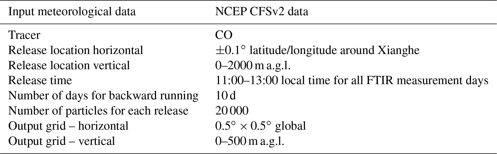
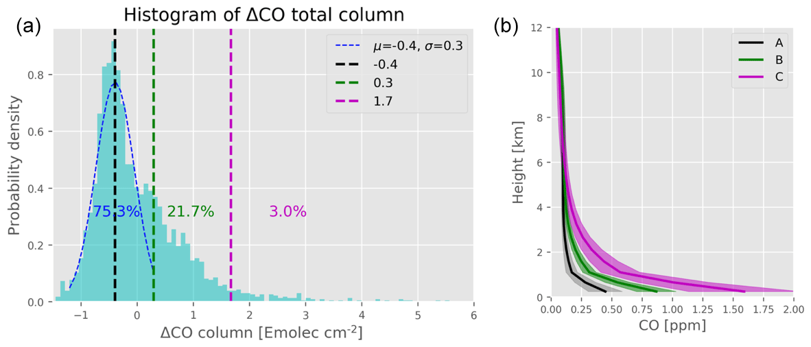
Figure 8 (a) The frequency density of the FTIR ΔCO distribution. Based on the highest density, we apply a normal distribution fitting ($\mathit{\mu }=-\mathrm{0.4}$ and σ=0.3). The ΔCO values that are less than μ+2σ, between μ+2σ and μ+6σ, and larger than μ+6σ are labeled as categories A (background), B, and C, respectively. The percentages of the categories A, B, and C are also indicated in the figure. (b) The vertical profiles of CO mole fraction within the three categories.

To better understand the air mass observed at Xianghe, the FTIR measurement days are classified into three categories (A, B, and C) according to different ΔCO levels. The background category A is selected as the following statistical method. Figure 8 shows the histogram of the ΔCO total column daily means at Xianghe. The dashed blue line is a Gaussian distribution ($\mathit{\mu }=-\mathrm{0.4}$ and σ=0.3) fitted to the left side of the highest probability density (dashed black line). The dashed green line denotes μ+2σ. The ΔCO on the left side together with the ΔCO on the right side of the black line with values that are less than μ+2σ generally follow the fitted Gaussian distribution, meaning that the ΔCO values below the dashed green line are selected as category A. The ΔCO distribution does not follow the Gaussian distribution when ΔCO is above the dashed green line. We use 4σ as the width (dashed purple line: μ+6σ) to divide high ΔCO values into categories B (between the dashed green and dashed purple lines) and C (on the right side of the dashed purple line). The percentages of categories A, B, and C are 75.3 %, 21.7 %, and 3.0 %, respectively. The mean and SD of the CO vertical profiles of the three categories are also shown in Fig. 8. As expected, a high variation in the CO mole fraction is observed in the lower troposphere. The CO mole fractions near the surface are about 0.4, 0.8, and 1.6 ppm in categories A, B, and C, respectively.

Figure 9 Spatial distributions of the air mass response sensitivity in 10 d backward simulations at Xianghe using the FLEXPART v10.4 model for all FTIR measurement days (All) and categories A, B, and C. Sensitivity is given in units of sm³ kg⁻¹. The Xianghe site is marked with a black dot. The values indicate the percentages of the emission response sensitivity larger than 50 (deep blue edge), 300 (cyan circle), and 1000 sm³ kg⁻¹ (red circle) .

Figure 9 shows the backward mean sensitivities for all the FTIR measurement days (701) and categories A (528 d), B (152 d), and C (21 d). In general, the air mass observed in the 0–2 km vertical range above Xianghe is mainly coming from the northwest direction, with about 66 % of the air mass sources in northern China and Mongolia. The high emission response sensitivity (cyan circle) for 300 km around Xianghe accounts for 28 % of the whole sensitivity dataset. Regarding category A, the major wind has a strong northwestern direction. In addition, less air mass comes from the region surrounding Xianghe. The air mass source inside the cyan circle takes up 26 %, and the air mass sources in northern China and Mongolia account for 60 %. The remaining 40 % of the air mass comes from northeastern China, Russia, Korea, Japan, central Asia, and Europe (not shown). For category B, the high emission response sensitivity area (cyan and red lines) is generally like a circle around Xianghe, with 40 % of the air mass coming from the cyan circle. The air mass sources in northern China and Mongolia account for 75 %. For category C, the air mass sources in northern China and Mongolia account for 89 %. The high emission response sensitivity area (cyan and red lines) has a northeast to southwest direction. The area inside the red circle has a high human activity level (Zhang et al., 2019), corresponding to large anthropogenic emissions.

In addition to the backward mean sensitivities, we also calculate the mean trajectory of all releasing particles of each model simulation. The mean and SD of the air mass height, distance away from the releasing site, and the wind speed and direction of the categories A, B, and C are shown in Fig. 10. The wind speed is much larger in category A compared to those in categories B and C, especially in the first 2 backward days. The major wind direction is northwest in category A, while the major wind directions are the west and southwest during the first 2 d in categories B and C, respectively. After the first 2 backward days, the wind directions for the three categories are generally the same: wind coming from the northwest. Due to the different wind conditions during the first 2 backward days, the air mass between 0 and 2 km observed at Xianghe is coming from the air mass about 500, 190, and 130 km away from the site at 1 d ago and about 1300, 520, and 410 km away from the site at 2 d ago for categories A, B, and C, respectively. In terms of the air mass height, large differences are found during the first 3 backward days where the air mass height is lower in category C and higher in category A. Our results show that the FTIR ΔCO total column level is strongly impacted by the local meteorological conditions. A high CO concentration is generally observed with a southwesterly wind direction, a wind speed below 10 km h⁻¹, and a more stable atmospheric condition.

Figure 10 The mean (solid line) and SD (shaded area) of the air mass height (a), the distance to the Xianghe site (b), and the wind direction and speed (c) of categories A, B, and C simulated by the FLEXPART 10 d backward running.

3.4 Fire emission observed by FTIR HCN measurements

The FTIR measurements observe a very strong HCN enhancement in August 2021, with the highest total column being 1.41 × 10¹⁶ molec. cm⁻² on 11 August (Figs. 5 and 11). Since HCN is a good tracer of fire emission, such enhancement might be related to a fire activity captured by the FTIR measurements at Xianghe. In this section, the Visible Infrared Imaging Radiometer Suite (VIIRS) data onboard the Suomi National Polar-orbiting Partnership (Suomi NPP) satellite (Schroeder et al., 2014) are applied to understand the fire spatial distribution during this period. The VIIRS/Suomi NPP satellite is capable of offering a complete coverage of the Earth during 1 d due to its large swath width of 3060 km. There are 22 spectral bands from 412 nm to 12 µm, among them five channels are imaging resolution bands (I-bands), which have a spatial resolution of 375 m at the nadir (Cao et al., 2014). In this study, we use the VIIRS 375 m fire datasets, which are downloaded from https://firms.modaps.eosdis.nasa.gov/ (last access: 13 January 2023). Note that we only select the fire pixels with confidence values equalling to normal and high. The fire data are then binned into 0.5^∘ × 0.5^∘ global grids, and the number of the individual fire pixels in each bin indicates the fire intensity.

Figure 11 Time series of the FTIR HCN total column measurements at Xianghe between 22 July and 25 August 2021. A total of 4 d of data (27 July, 4 August, 11 August and 18 August) are used to understand the air mass sources (see Fig. 12) and are marked with the dashed black lines.

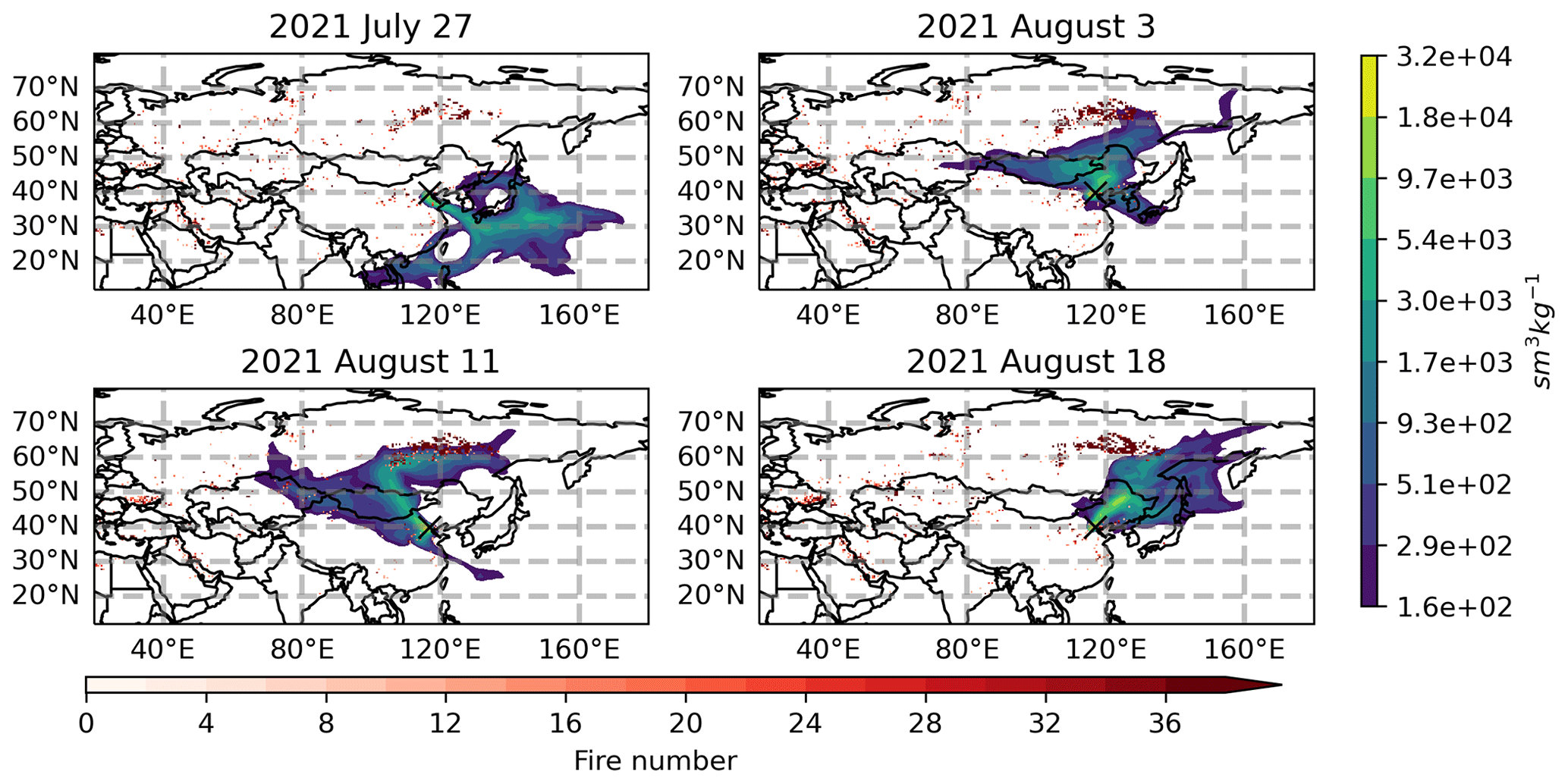
Figure 12 Spatial distributions of the air mass response sensitivity in 10 d backward simulations at Xianghe using the FLEXPART v10.4 model on 27 July, 4 August, 11 August, and 18 August 2021. The air is treated as a trace gas, and 20 000 particles are released at 0–2 km above Xianghe in the temporal window of ±1 h around the local noon. Xianghe site is remarked as the black cross. The fire counts are observed by the VIIRS/Suomi NPP satellite, and all individual fires within 1 to 10 d before each air mass release day are summed up and binned into 0.5^∘ × 0.5^∘ global grids.

Figure 12 shows the air mass response sensitivity from the FLEXPART backward simulations on four HCN measurement days (27 July: low HCN column about 2 weeks before the peak; 3 August: 1 week before the peak; 11 August: the peak; 18 August: 1 weak after the peak), together with the fire counts observed by the VIIRS satellite. Similar to Sect. 3.3, the air mass is released at 0–2 km above Xianghe in the temporal window of ±1 h around local noon. Note that in this section we use the air as the trace gas instead of CO, and the vertical output grid is set to 0–5 km a.g.l. instead of 0–500 m a.g.l. All the individual fires within 1 and 10 d are summed up before each air mass releasing day. For example, the fire number map on 27 July 2021 is derived from all the fires between 18 and 26 July 2021. Figure 12 shows that the area burned in the boreal forest of Russia (Siberia) between the end of July and August 2021 is related to the FTIR HCN peak. On 27 July, the air mass observed at Xianghe is coming from the southeast (Pacific Ocean). Since the air in the Pacific Ocean is clean, the HCN total column on that day is very low at 0.52 × 10¹⁶ molec. cm⁻². In the boreal forest region of Russia (Siberian and Far Eastern districts), we notice that there are several fire counts. On 3 August, the fire area in Siberia became large, and the air mass observed at Xianghe changed its main direction from southeast to northeast. However, only a small portion of the fire emission was transported and observed by the FTIR measurements at Xianghe, with an HCN total column of 0.69 × 10¹⁶ molec. cm⁻². On 11 August, the fire area in Siberia remained large but moved slightly to the south, and the air mass observed at Xianghe captured the fire emission well. As a result, the FTIR measurements observe the HCN total column peak. On 18 August, the boreal forest fire area got smaller and moved towards the north. The air mass observed at Xianghe is coming from the northeast, which only covers a part of the fire region. The HCN total column observed by the FTIR measurements decreases to 0.87 × 10¹⁶ molec. cm⁻². Based on the satellite fire measurements and FLEXPART back simulations, we understand that the drop in HCN columns in July 2021 is due to the air mass coming from the Pacific Ocean, and the peak in HCN columns in August 2021 is due to the boreal forest fire emission in the Siberia.

In fact, we can also observe enhancements in CO, C₂H₂, and C₂H₆ columns in August 2021 (Fig. 5), although their amplitudes are not as significant as HCN. We do not observe any increase in H₂CO columns at Xianghe on 11 August, which is due to the fire emissions being less important for H₂CO and as the lifetime of H₂CO is only a few hours (Table 1). The enhanced amplitudes in August 2021 are 1.65 × 10¹⁸ molec. cm⁻² for CO, 5.57 × 10¹⁵ molec. cm⁻² for C₂H₂, and 1.91 × 10¹⁶ molec. cm⁻² for C₂H₆, respectively, which account for 39 %, 42 %, and 66 % of their largest enhancements caused by the local anthropogenic emissions, respectively. To conclude, the enhancements of CO, C₂H₂, and C₂H₆ at Xianghe, resulting from the fire emissions being less significant compared to the local anthropogenic emissions, and the enhancements in CO, C₂H₂, and C₂H₆ caused by the fire emissions are less significant compared to HCN. This indicates that HCN (but not the other three species) is a good trace gas for fire emissions in northern China. The major emissions of CO, C₂H₂, and C₂H₆ at Xianghe do not come from fire emissions but come from local anthropogenic emissions.

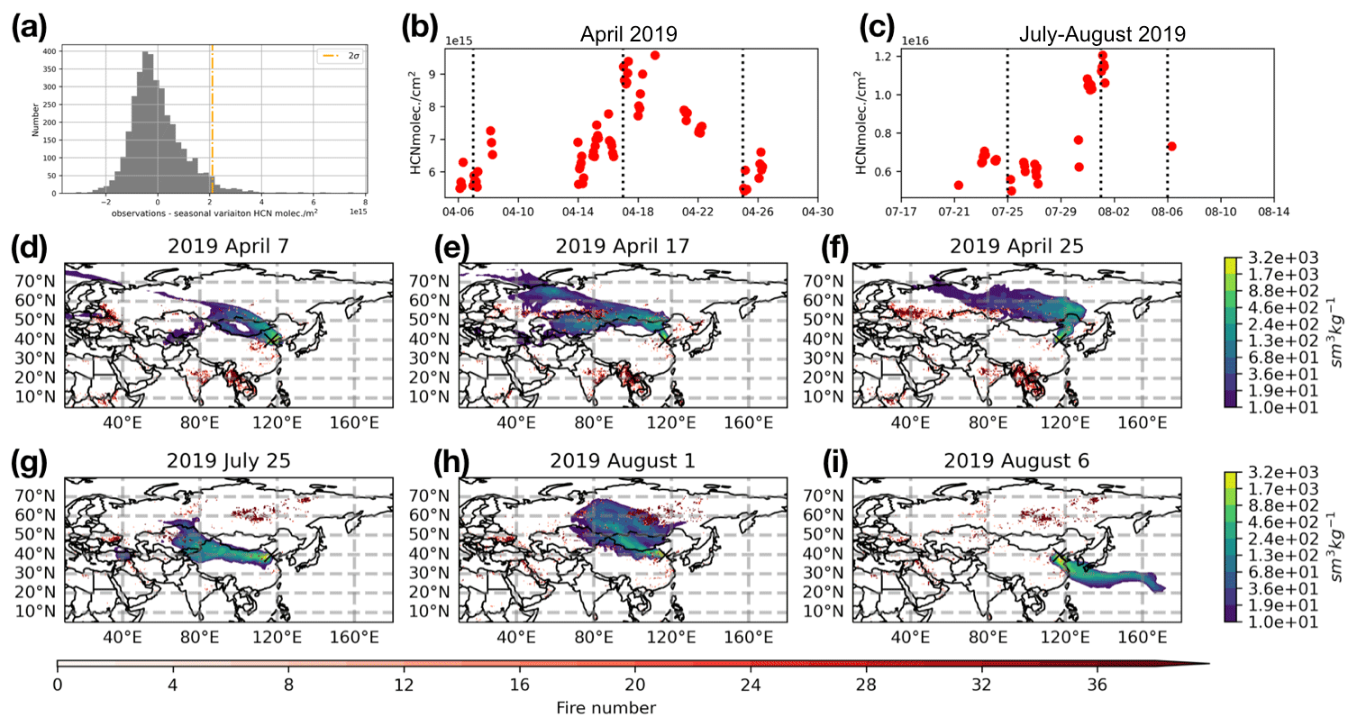
Figure 13 The frequency density of the FTIR HCN column variation (observations minus seasonal variation) (a). The time series of the FTIR HCN total column measurements at Xianghe between 6 and 30 April 2019 (b) and between 17 July and 14 August 2019 (c). For each period, 3 d (approximately 1 week before the peak, the peak, and 1 week after the peak) are used to understand the air mass sources for each HCN enhancement period and shown as dashed black lines. The spatial distributions of the air mass response sensitivity in 10 d backward simulations at Xianghe using the FLEXPART v10.4 model (similar to Fig. 10) on 7 April (d), 17 April (e), 25 April (f), 25 July (h), 1 August (i), and 6 August 2019 (j).

Apart from August 2021, can we also see the fire emission in other years? Figure 13a shows the histogram distribution of the FTIR HCN column deviations (observations minus seasonal variation). To identify the fire emission periods, we select all the HCN deviation larger than 2σ (on the right side of the vertical orange line). To further reduce the measurement uncertainty, we take the HCN-enhanced day with at least three individual measurements. As a result, we find another two periods (17 to 19 April and 31 July to 1 August 2019) to investigate the fire emissions (Fig. 13b and c). The enhancements of HCN in these two periods are less than that in August 2021. With the same method, the FLEXPART simulations and VIIRS satellite fire measurements are able to identify the fire emission sources (Fig. 13d–i). It is found that the enhancement of HCN in April 2019 is related to the nearby fire emissions in Kazakhstan and Russia, and the enhancement of HCN in July and August 2019 is related to the fire emissions in Siberia, Russia.

3.5 Emission estimation for C₂H₂ and C₂H₆

The relationship of CO with NMHCs can provide useful information on the anthropogenic emissions (Wang et al., 2004; Liu et al., 2014). The high correlations among ΔCO, ΔC₂H₂, and ΔC₂H₆ at Xianghe indicate that these species are commonly emitted from the surrounding sources. The FLEXPART model simulations show that the day-to-day variation in CO, C₂H₂, and C₂H₆ (Δgas) is insensitive to atmospheric transport, as the emissions are dispersed in a similar manner by the wind. Therefore, the impact of transport cancels out in the ratio. The change in meteorological conditions is typically within 3–5 d, which is much shorter compared to the lifetime of CO, C₂H₂, and C₂H₆. Moreover, as Xianghe site is inside the anthropogenic emission region, the large enhancements of ΔCO, ΔC₂H₂, and ΔC₂H₆ are directly coming from the local emissions, and the effect of OH sink is limited. Consequently, FTIR-observed ratios of ΔCO to ΔC₂H₂ (or ΔC₂H₆) at Xianghe (Fig. 6) can directly link to emission ratios

$$\begin{array}{}\text{(8)}& {\displaystyle \frac{E_g}{E_{\mathrm{CO}}}}={\displaystyle \frac{\mathrm{\Delta }{\mathrm{FTIR}}_g{M}_g}{\mathrm{\Delta }{\mathrm{FTIR}}_{\mathrm{CO}}{M}_{\mathrm{CO}}}},\end{array}$$

where E_CO is the emission of CO, M_CO is the molecular mass of CO, and subscript g represents C₂H₂ or C₂H₆. Note that H₂CO and HCN are not discussed here because H₂CO is mainly generated from chemical reactions from CH₄ instead of the direct anthropogenic emission, and HCN is strongly affected by the fire emissions apart from anthropogenic emission.

Once we know the emission of CO, the emission of C₂H₂ or C₂H₆ can then be estimated based on Eq. (8). According to the FLEXPART backward simulation, we understand that the air mass observed by the FTIR measurements at Xianghe is mainly from northern China and Mongolia (Fig. 9). Here, we use the 66 % of air mass response sensitivity for all FTIR measurement days (all in Fig. 9) as the FTIR sensitive emission area (FSEA). Four global and regional inventories (EDGAR v5.0, REAS v3.2, Peking University emission inventory (PKU; Zhong et al., 2017), and Multi-resolution Emission Inventory for China (MEIC) v1.3; Li et al., 2017) are applied to calculate the CO emission in the FSEA. Since these inventories have no data in 2018–2021, we use the latest available year for each dataset (EDGAR v5.0 and REAS v3.2 are 2015 annual means, PKU is the 2014 annual mean, and MEIC v1.3 is the 2017 annual mean). Apart from the CO emission, the C₂H₂ and C₂H₆ emissions are also provided by the EDGAR v4.3.2 for 2012 annual mean and the REAS v3.2 for the 2015 annual mean.

Table 6 The anthropogenic emissions of CO in the FSEA from EDGAR v5.0 and REAS v3.2 in 2015, PKU in 2014, and MEIC v1.3 in 2017. C₂H₂ and C₂H₆ emissions are derived from the FTIR measurements at Xianghe together with the CO emissions.

^a C₂H₂ and C₂H₆ emissions are from EDGAR v4.3.2 in 2012. ^b C₂H₂ and C₂H₆ emissions are from REAS v3.2 in 2015.

Table 6 lists the CO emissions in the FSEA from the four inventories, and the corresponding C₂H₂ and C₂H₆ emissions calculated from the FTIR measurements using Eq. (8) for these inventories. It is noted that the CO emissions in the FSEA from these four inventories, particularly in northern China, have a wide range from 36.8 to 80.6 Mt yr⁻¹, which agrees well with the previous study (Zheng et al., 2018). As a result, the C₂H₂ and C₂H₆ anthropogenic emissions are estimated to be 0.08–0.17 and 0.18–0.39 Mt yr⁻¹, respectively. The C₂H₂ and C₂H₆ anthropogenic emissions from EDGAR v4.3.2 are both 0.24 Mt yr⁻¹, meaning that the C₂H₂ emission is larger than the result derived from the FTIR measurements and the C₂H₆ emission is close to the result derived from the FTIR measurements. The C₂H₂ and C₂H₆ anthropogenic emissions from REAS v3.2 are 0.11 and 0.12 Mt yr⁻¹, respectively. In contrast to EDGAR v4.3.2, the REAS v3.2 C₂H₂ emission is close to the result derived from the FTIR measurements, but the REAS v3.2 C₂H₆ emission is underestimated as compared to the result derived from the FTIR measurements.

4 Conclusions

The variations and correlations of CO, C₂H₂, C₂H₆, H₂CO, and HCN columns in a polluted region in northern China are investigated based on the new FTIR measurements at Xianghe between June 2018 and November 2021. CO, C₂H₂, C₂H₆, H₂CO, and HCN columns are retrieved by the SFIT4 code followed by the NDACC-IRWG protocols. The retrieval strategies, retrieval information, and retrieval uncertainties of these species are also discussed. For all of these species, the retrieved profile has good sensitivity in the troposphere. According to the DOFS, there are more than two pieces of independent information in CO and HCN, mainly the column information in C₂H₂, C₂H₆, and H₂CO. In this study, we mainly focus on the total columns, and the systematic and random uncertainties of CO, C₂H₂, C₂H₆, H₂CO, and HCN columns are 2.1 ± 1.6 %, 6.0 ± 7.9 %, 3.5 ± 2.4 %, 6.0 ± 6.0 %, and 12.9 ± 2.9 %, respectively.

The mean and SD are 2.86 ± 0.87 × 10¹⁸, 0.60 ± 0.29 × 10¹⁶, 3.02 ± 0.70 × 10¹⁶, 1.26 ± 0.91 × 10¹⁶, and 0.57 ± 0.14 × 10¹⁶ molec. cm⁻² for CO, C₂H₂, C₂H₆, H₂CO, and HCN columns, respectively. The seasonal variations in C₂H₂ and C₂H₆ total columns show a maximum in winter–spring and a minimum in autumn, and the seasonal variations in H₂CO and HCN show a maximum in summer and a minimum in winter. We find that there is no clear seasonal variation in the CO total column, with a month-to-month variation of less than 5 % (consistent with TROPOMI satellite measurements and TCCON measurements). The weak seasonal variation in the CO column at Xianghe is very different from other FTIR sites, such as Paris and Hefei, which is probably due to a large CH₄ value in summer at Xianghe (Ji et al., 2020; Yang et al., 2020) and a short distance between the Xianghe FTIR site and the local anthropogenic sources.

The FLEXPART model is applied to understand the air mass sources observed by the FTIR measurements at Xianghe. It is found that the high values of these species are mainly coming from the local anthropogenic emissions in northern China. With a strong wind speed (typically larger than 20 km h⁻¹ at 1 km a.g.l) and northwesterly wind direction, the FTIR measurements show lower values. Together with the VIIRS satellite fire measurements, we found that the fire emissions in boreal forest (Kazakhstan and Russia) can transport to Xianghe and be captured well by our FTIR measurements, leading to a strong enhancement in FTIR HCN columns. The FTIR HCN column is a good tracer for fire emissions in northern China, but the other four species do not show the same relationship. The major emissions of CO, C₂H₂, and C₂H₆ at Xianghe come from local anthropogenic emissions. The high correlations between CO, C₂H₂, and C₂H₆, with R between 0.70 and 0.80, indicate that they are affected by the common sources. We use the slopes observed by the FTIR measurements to estimate their emissions. Based on four global and regional CO emission inventories (EDGAR v5.0, REAS v3.2, PKU, and MEIC v1.3), the CO emission in the FSEA (northern China and Mongolia) is between 36.8 and 80.6 Mt yr⁻¹. The C₂H₂ and C₂H₆ anthropogenic emissions in the FSEA are estimated to be 0.08–0.17 and 0.18–0.39 Mt yr⁻¹, respectively.

The CO, C₂H₂, C₂H₆, H₂CO, and HCN FTIR column measurements at Xianghe are helpful to investigate the air quality in northern China. Although at the moment the time coverage is still too short to understand their long-term trend, the ongoing FTIR measurements at Xianghe can help us to study Chinese air pollution improvements, long-distance fire emissions transportation, satellite calibration and validation, and model verification.

Appendix A: TCCON and TROPOMI CO measurements at Xianghe

The FTIR NDACC-type measurements at Xianghe show that the seasonal variation in the CO total column is very weak, which is very different from other FTIR sites. The TCCON measurements are also operated at Xianghe using the same Bruker IFS 125HR spectrometer (Yang et al., 2020). Here, we check the dry air column average mole fraction of CO (XCO) time series and seasonal variation from the TCCON measurements (GGG2020) at Xianghe. Moreover, we also select the TROPOMI overpass offline CO column data (Borsdorff et al., 2019) within 50 km around the Xianghe site between June 2018 and November 2021 (https://scihub.copernicus.eu/, last access: 13 January 2023). The spatial resolution of the TROPOMI measurement is 7.0 × 7.0 km² before 6 August 2019 and 7.0 × 5.5 km² afterwards. Figure A1 shows the time series and seasonal variation in the CO column observed by the TCCON and TROPOMI satellite at Xianghe. Both TCCON and TROPOMI measurements show that the seasonal variation in the CO column at Xianghe is hardly observed. The amplitudes of the fitted seasonal variation derived from the TCCON and TROPOMI measurements at Xianghe are within 6 %, which is similar to the ground-based FTIR NDACC-type measurements.

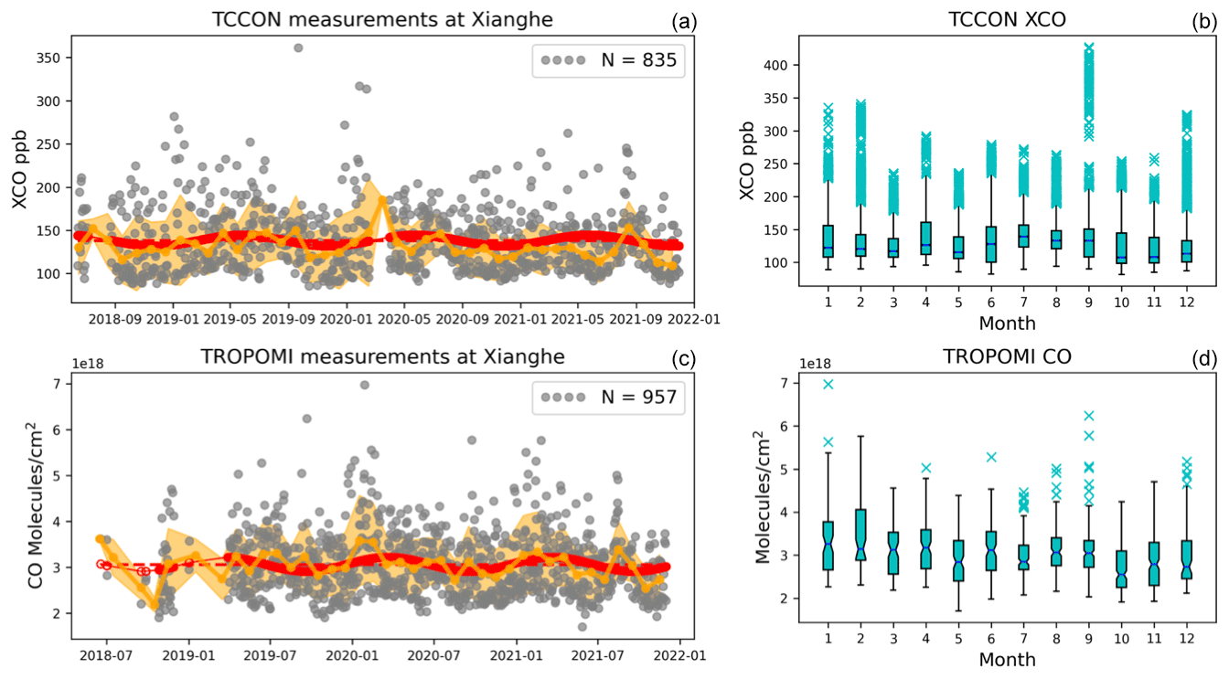
Figure A1 (a, c) Time series of XCO and CO columns observed by TCCON at Xianghe (a) and TROPOMI overpass within 50 km around Xianghe (c) between June 2018 and November 2021. Gray dots are daily means with the total number indicated by N, the dotted orange line is the monthly mean, the shaded yellow area is the monthly standard deviation, the dashed red line is the offset A₀ (almost overlapping with the solid red line), and the solid red line is the fitted time series y(t). (b, d) The monthly box plot of the CO columns in each month. The bottom and upper boundaries of the box represent the 25 % (Q1) and 75 % (Q3) percentile of the data points around the median value, the error bars extend no more than 1.5 × IQR (IQR = Q3 − Q1) from the edges of the box, and the blue crosses are the extremely low and high values.