A novel, cost-effective analytical method for measuring high-resolution vertical profiles of stratospheric trace gases using a gas chromatograph coupled with an electron capture detector

The radiative balance of the upper atmosphere is dependent on the magnitude and distribution of greenhouse gases and aerosols in that region. Climate models predict that with increasing surface temperature, the primary mechanism for transporting tropospheric air into the stratosphere (known as the Brewer–Dobson circulation) will strengthen, leading to changes in the distribution of atmospheric water vapor, other greenhouse gases, and aerosols. Stratospheric relationships between greenhouse gases and other long-lived trace gases with various photochemical properties (such as N₂O, SF₆, and chlorofluorocarbons) provide a strong constraint for tracking changes in the stratospheric circulation. Therefore, a cost-effective approach is needed to monitor these trace gases in the stratosphere. In the past decade, the balloon-borne AirCore sampler developed at NOAA's Global Monitoring Laboratory has been routinely used to monitor the mole fractions of CO₂, CH₄, and CO from the ground to approximately 25 km above mean sea level. Our recent development work adapted a gas chromatograph coupled with an electron capture detector (GC-ECD) to measure a suite of trace gases (N₂O, SF₆, CFC-11, CFC-12, H-1211, and CFC-113) in the stratospheric portion of AirCores. This instrument, called the StratoCore-GC-ECD, allows us to retrieve vertical profiles of these molecules at high resolution (5–7 hPa per measurement). We launched four AirCore flights and analyzed the stratospheric air samples for these trace gases. The results showed consistent and expected tracer–tracer relationships and good agreement with recent aircraft campaign measurements. Our work demonstrates that the StratoCore-GC-ECD system provides a low-cost and robust approach to measuring key stratospheric trace gases in AirCore samples and for evaluating changes in the stratospheric circulation.

1 Introduction

Monitoring the dry-air mole fractions of a suite of trace gases in the stratosphere will significantly improve our understanding of the stratospheric mean meridional circulation's (Brewer–Dobson circulation or BDC) response to changing climate. The BDC is characterized by upwelling in the tropics, with upper and lower poleward branches and descent in the extra-tropics (Holton et al., 1995; Garcia and Randel, 2008; Butchart, 2014). Coupled chemistry–climate models (CCMs) predict an acceleration of the BDC in response to increasing greenhouse gas abundances and surface temperatures (Butchart et al., 2006; Garcia and Randel, 2008; McLandress and Shepherd, 2009; Butchart, 2014), with far-reaching implications for surface weather, earth's radiation budget, and the climate (Forster and Shine, 2002; Randel et al., 2006; Gerber et al., 2012); recovery of the stratospheric ozone layer (Butchart and Scaife, 2001; Butchart et al., 2010); and potential impacts to surface air quality due to changes in stratosphere-to-troposphere ozone flux (Hegglin and Shepherd, 2009). Furthermore, evaluating the impact of potential future climate intervention techniques also requires accurate modeling of the BDC in CCMs. However, directly measuring the strength and variation in the BDC is difficult.

The mean age of air (AoA) in the stratosphere (Ray et al., 1999; Andrews et al., 2001; Waugh and Hall, 2002) has been suggested to be an indicator of the BDC strength (Engel et al., 2009; Stiller et al., 2012, 2017). The measurement-derived AoA, traditionally using mole fractions of carbon dioxide (CO₂) and sulfur hexafluoride (SF₆), can be compared with modeled AoA to investigate the model's performance in simulating the BDC. However, later studies showed that the BDC is not the only factor controlling the mean AoA, as it is also affected by the mixing of air from the extra-tropics back into the tropics, i.e., recirculation (Ray et al., 2014; Garny et al., 2014; Ploeger et al., 2015; Dietmüller et al., 2017). Also, recent work has shown that SF₆ has a non-negligible chemical sink in the mesosphere (Ray et al., 2017; Leedham Elvidge et al., 2018; Loeffel et al., 2022), biasing AoA calculations that rely on SF₆ mole fractions alone. Since the mesospheric SF₆ loss rate is proportional to its mole fraction, which has been increasing rapidly in the past few decades, the measured SF₆ mole fraction in the midlatitudes now contains measurable information not only about AoA but also about the mass exchange between the stratosphere and the mesosphere, which was only obtainable in polar vortex profiles before. Additional work has shown that the stratospheric dry mole fractions of some long-lived trace gases, such as nitrous oxide (N₂O), and several chlorofluorocarbons (CFCs), including dichlorodifluoromethane (CFC-12), trichlorofluoromethane (CFC-11), 1,1,2-trichloro-1,2,2-trifluoroethane (CFC-113), and bromochlorodifluoromethane (halon 1211 or H-1211), could provide further constraints to help better understand stratospheric circulation and transport pathways of air into the stratosphere (Volk et al., 1996; Strahan et al., 1999; Schoeberl et al., 2000; Moore et al., 2014). This is because (1) photolytic destruction is the sole sink for these gases, (2) their photolytic destruction rates increase exponentially with altitude, and (3) the altitude–photolytic lifetime profiles for these trace gases are different (Moore et al., 2014). Therefore, observations of a suite of tracers are needed to carefully monitor, examine, and verify simulated stratospheric transport.

The lightweight balloon-borne observation system known as the AirCore provides a low-cost approach to observing the composition of the stratosphere (Tans, 2009; Karion et al., 2010). High-quality in situ measurements of stratospheric air are rare, since the cost of such field campaigns prohibits routine measurements. As a result, data collected from occasional high-altitude large-balloon (>10⁶ m³) and aircraft-based field campaigns since the 1980s are still relevant today for diagnosing stratospheric composition and dynamical change (Hall et al., 1999; Andrews et al., 2001; Pan et al., 2010; Laube et al., 2020). The AirCore was developed at the NOAA Global Monitoring Laboratory (NOAA/GML) and has been widely used to measure CO₂, CH₄, and CO profiles in samples collected from the surface to the stratosphere. The AirCore consists of a long (approximately 100 m), thin, coated stainless steel tube with one open end. The gas in the AirCore flows out as it ascends on a balloon. After the balloon is cut away at 30–32 km above mean sea level (AMSL), the AirCore descends and passively collects ambient air. Due to the relatively low volumetric flow rate and small cross-section area of the AirCore, the mixing of air captured in the AirCore is limited to Taylor dispersion (Aris, 1956) and molecular diffusion, largely preserving the vertical structure of the atmosphere in the AirCore (Tans, 2009; Karion et al., 2010). After landing, the AirCore automatically closes, preserving the collected air sample until laboratory analysis. As AirCores are usually analyzed shortly (less than 4 h) after landing, the composition of air from the ground to the mid-stratosphere can be measured with only a small amount (less than 0.7 m in both directions, Karion et al., 2010) of diffusion and dispersion mixing of the sample, allowing for the retrieval of vertical gradients of trace gases in air from the ground to the mid-stratosphere with significant fidelity at a relatively low cost (USD 5000 per profile).

The most common analytical approach for analyzing AirCore samples employs continuous-flow gas analyzers to derive the vertical profiles of CO₂, CO, CH₄, and N₂O (Karion et al., 2010; Membrive et al., 2017; Engel et al., 2017). In this approach, the AirCore sample is pushed through one, or a series of, continuous-flow gas analyzer(s), during which the analyzer(s) measure the dry mole fractions of several gases (CO, CO₂, N₂O, and CH₄) at a relatively slow flow rate (approximately 30 mL min⁻¹) and data rate of approximately 0.45 Hz. These measurements are then combined with flight data (such as altitude, pressure, and temperature) to derive vertical profiles of measured trace gases with altitude, using estimates of flow impedance due to flow resistance in a laminar regime as sample air moves along the length of tubing (Tans, 2022). Although this method provides fast, high-resolution measurements of several essential trace gases, the continuous analyzers cannot directly measure other trace gases of interest for evaluating changes in the BDC (such as CFCs or SF₆), limiting the species measured from an AirCore sample. Mrozek et al. (2016) and Laube et al. (2020) have designed subsampling systems that separate the AirCore samples into 20–30 mL aliquots, allowing for more detailed chemical and isotopic measurements using non-continuous-flow analytical instruments. This method was then applied to measure the dry mole fractions of CFC-11 and other trace gases in each subsample and to investigate mass-independent fractionation in CO₂ (Mrozek et al., 2016; Laube et al., 2020). However, subsampling from AirCores only allows for a limited number of stratospheric measurements per small AirCore sample volume. In the case of Mrozek et al. (2016), 10 stratospheric measurements from a 2 L volume AirCore can be measured in each flight. With the weight of NOAA unmanned free balloon payloads limited to 5.4 kg by the Federal Aviation Administration (FAA) in the United States, the subsampling method would provide lower vertical resolution and thus limited utility in resolving critical stratospheric gradients of these gases. Additionally, NOAA's AirCore sampling program routinely deploys two samplers simultaneously, which currently restricts the total volume of each AirCore to less than 1 L. Therefore, an alternative approach is needed to measure the mole fractions of several critical trace gases in AirCores using a smaller sample volume per measurement.

Here, we present a novel analytical method using a modified gas chromatograph coupled with an electron capture detector (GC-ECD) system to analyze the dry mole fractions of CFC-11, CFC-12, CFC-113, H-1211, N₂O, and SF₆ from the stratospheric portion of AirCore samples (approximately the first 20 %–30 % of the sampler tubing). We name this system the StratoCore-GC-ECD. The StratoCore-GC-ECD is designed to accomplish high-precision measurements of these six species using only ∼4–5 mL of air sample per measurement from the stratospheric portion of AirCores while carefully registering the altitude information of each data point, allowing us to acquire high-resolution measurements of the vertical gradient of these trace gases from the tropopause to the mid-stratosphere. This analytical method offers the potential for long-term monitoring of these gases using a balloon-borne sampling package that is regulated under the same flight rules as those that apply to weather balloons. This methodology, coupled with the AirCore, will provide us the flexibility to measure important stratospheric tracers at an enhanced spatial and temporal resolution over current analytical methods. Such observations will provide us with valuable information to monitor a suite of trace gases in the stratosphere long term at low cost, define baseline stratospheric conditions for any perturbations in stratospheric composition due to future climate intervention techniques, and provide observational evidence to detect and monitor changes in the BDC.

2 The StratoCore-GC-ECD setup

2.1 Gas chromatography

The sample analysis portion of the StratoCore-GC-ECD system is adopted from previous GC systems designed and built for rapid, high-frequency in situ analysis on aircraft and large-balloon platforms (Elkins et al., 1996; Romashkin et al., 2001; Moore et al., 2003; Hintsa et al., 2021). Figure 1 displays a diagram of the StratoCore-GC-ECD system. The analysis component consists of a two-channel GC-ECD that mimics the design of the UAS Chromatograph for Atmospheric Trace Species (UCATS; Hintsa et al., 2021) and the in situ GC system used during the Lightweight Airborne Chromatograph Experiment campaign (LACE; Moore et al., 2003). The GC system uses ultra-high purity nitrogen (N₂) as the carrier gas. In each GC channel, a Valco 12-port two-position valve (VICI, TX, USA) is used to switch between sample loading (into two 1 mL sample loops) and injecting modes. Each analysis takes 120 s in this setup. Channel 1 uses a 10 % dimethylsilicone (OV-101) packed column as the pre-column to separate CFC-12, H-1211, CFC-11, and CFC-113 in the sample, which subsequently passes through the main column and is analyzed by the ECD detector. A temperature controller (model CNI16-AL, Omega, CT, USA) is used to control column temperature at 38 ^∘C. The flow rate of carrier gas in this channel is 70 mL min⁻¹, and the pre-column is backflushed for 85 s at 100 mL min⁻¹ in each analysis to remove the residual sample. Similarly, Channel 2 uses HayeSep^® D porous polymer packed columns followed by Molecular Sieve 5A to separate SF₆ and N₂O (controlled at 110 ^∘C), which are then analyzed by the second ECD detector. The carrier gas flow rate in Channel 2 is 70 mL min⁻¹. Backflushing in Channel 2 occurs after 55 s of each 120 s analysis at 100 mL min⁻¹ to remove any residual sample. In addition, a small flow of pure CO₂ (0.2,mL min⁻¹) is mixed into the ECD detector in Channel 2 as a dopant to minimize the matrix effect and improve the ECD response to N₂O (Fehsenfeld et al., 1981).

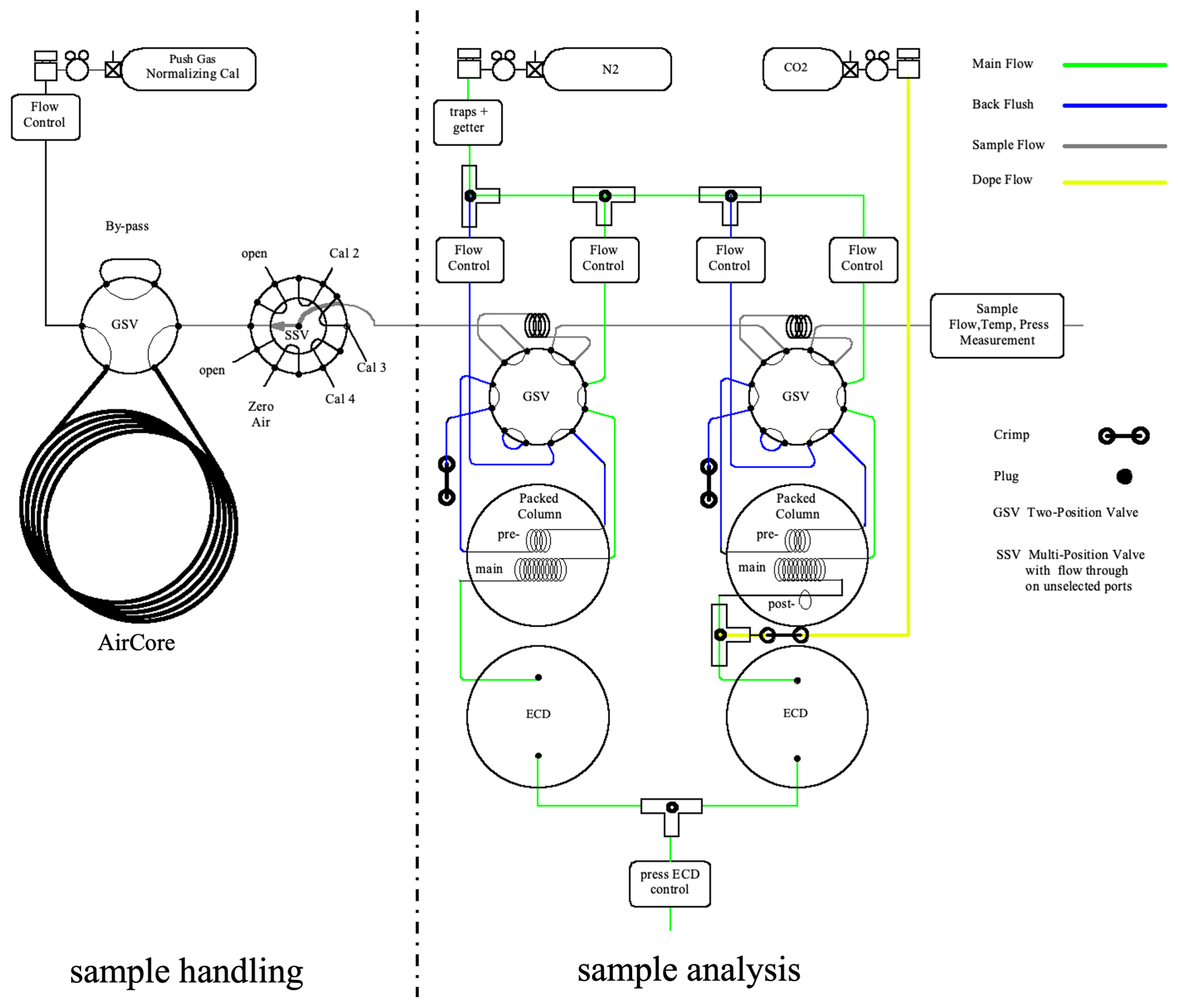
Figure 1 Simplified sketch of the StratoCore-GC-ECD system. The dashed line marks the boundary between the sample handling system and the sample analysis system. Left of the dashed line is the sample handling system, which carefully injects the sample from AirCores (4–5 mL per analysis) into the GC-ECD. Right of the dashed line is the sample analysis system, which measures the mole fractions of six trace gases in each injection.

The StratoCore-GC-ECD system displays adequate analytical precisions suitable for measuring the dry-air mole fractions of CFC-11, CFC-12, CFC-113, H-1211, N₂O, and SF₆ (hereafter referred to as target molecules) in the stratosphere. Typical chromatographs are shown in Fig. 2. The analytical repeatability of the GC-ECD for the target molecules is evaluated by measuring gas cylinders with well-determined dry mole fractions of target molecules multiple times, and the uncertainties are shown in Table 1. Considering the dry mole fractions of these species in the stratosphere display wide ranges (50 %–100 % overall variations for CFCs and N₂O, 20 % for SF₆), such analytical precisions (<0.7 %) of the GC-ECD should be sufficient to understand the stratospheric variability of these species. A set of five gas mixtures in Aculife-treated aluminum cylinders, spanning the range of expected stratospheric dry-air mole fractions (20 % to 100 % of tropospheric values), were prepared and used to calibrate the GC-ECD. Examples of the most recent calibration curves are shown in Fig. 3. Furthermore, as new trace gas species emerge and grow in the atmosphere, identifying possible interferences caused by the GC co-elution of target molecules and potential new trace gases is important. We therefore tie the StratoCore-GC-ECD measurements to the surface network program at NOAA/GML, where atmospheric samples are analyzed on both GC-ECD and GC-MS. The intercomparisons between the different analytical techniques could be used to detect potential interferences if they emerge in the future.

Table 1 Analytical repeatability of the StratoCore-GC-ECD, reported relative to the tropospheric mole fraction of each gas.

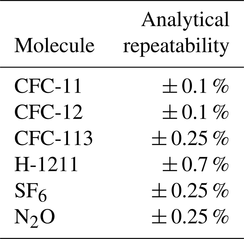
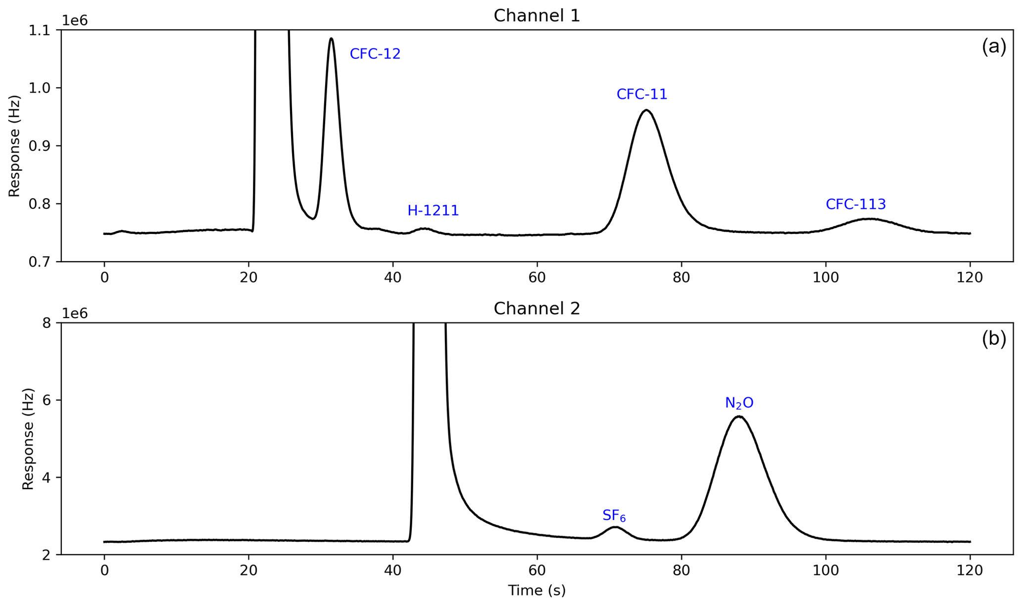
Figure 2 A typical chromatogram from StratoCore-GC-ECD analysis. The x axis is the retention time of each analysis, and the y axis is the response of the ECD. The top panel is the response of Channel 1 (analyzing the mole fractions of CFC-12, H-1211, CFC-11, and CFC-113), and the bottom panel is the response of Channel 2 (analyzing the mole fractions of N₂O and SF₆).

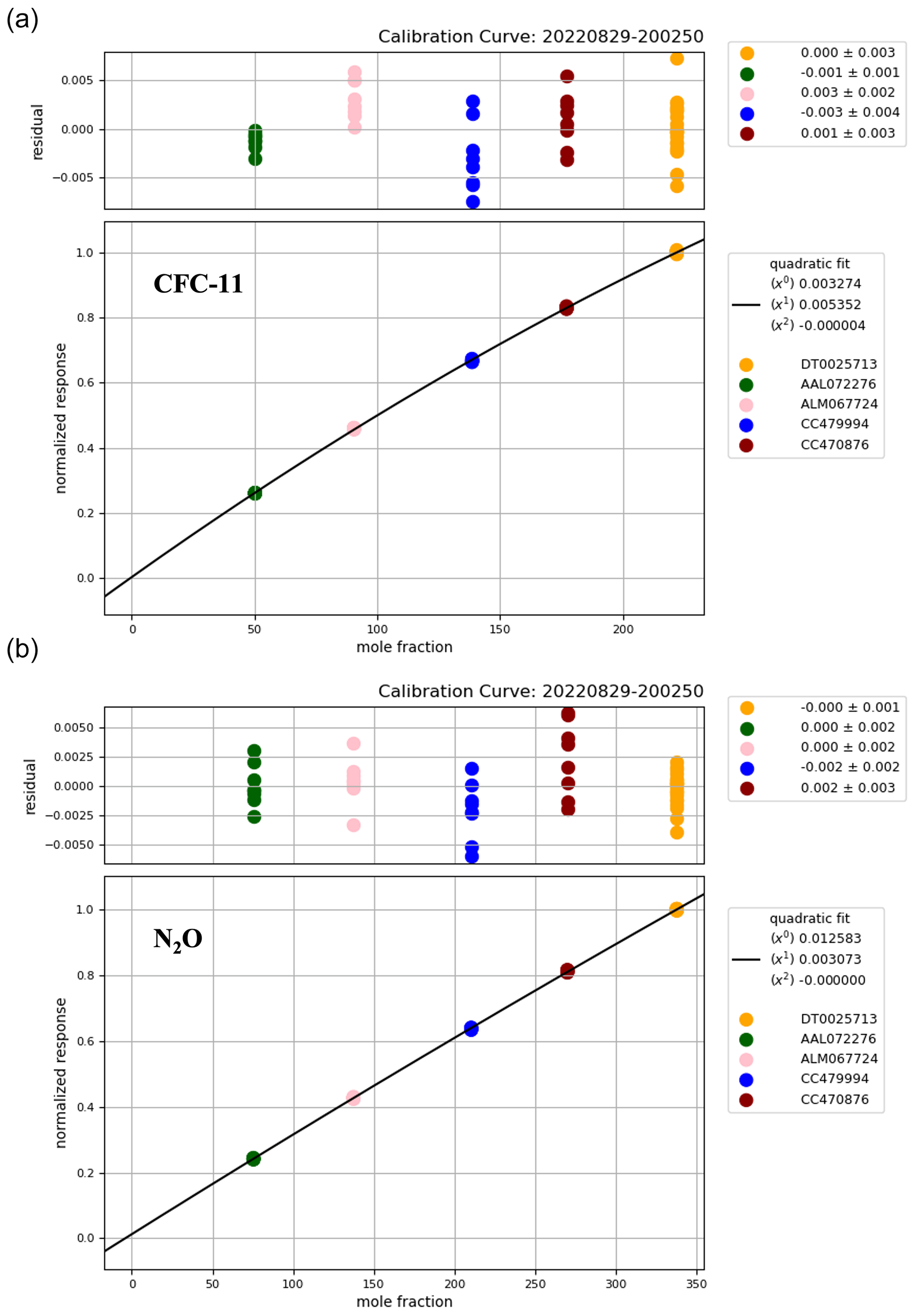
Figure 3 Examples of calibration curves ((a): CFC-11, (b): N₂O) generated by analyzing five standard tanks using the StratoCore-GC-ECD system. Each color represents a different calibration tank, and each tank was measured a total of seven times. In each panel, the upper figure shows the relative residual mole fraction (unitless) between the measured value and the true curve, and the legend shows the mean residual of each tank; the lower figure shows the calibration curve and the parameters of the quadratic fit function, and the legend shows the standards used.

2.2 Sample handling

Airborne in situ GC-ECD systems typically use a high sample flow (∼100 mL min⁻¹) to flush the sample loading system prior to analysis (Elkins et al., 1996; Romashkin et al., 2001; Moore et al., 2003; Hintsa et al., 2021). However, the limited amount of AirCore sample (here, < 250 mL of air) requires an alternative approach to load air into the GC-ECD. To achieve this goal, an in-house sample handling system was specially designed and built to capture and inject sample gas from the AirCore into the GC-ECD system (Fig. 1). The flow path in the sample handling system is controlled by a six-port two-position valve, and AirCore samples are carefully pushed at low pressure (approximately 300 hPa above ambient pressure) by an in-house standard gas cylinder with well-determined dry mole fractions of target molecules. The six-port valve setup allows this “push gas” to also act as a calibration standard that can be directly injected into the GC-ECD periodically (through the bypass position, Fig. 1). For each sample loading, the sample flow rate is controlled by a mass flow controller (Mykrolis, MA, USA) at 4–5 mL min⁻¹ to maintain a stable pressure profile and constant flow. The flow rates during the sample loading process are then measured by a mass flow meter (Omega, CT, USA) at 1 Hz at the outlet of the StratoCore-GC-ECD system with a precision better than 0.6 % (see Sect. 2.3). The flow measurements associated with each sample loading process are integrated to calculate the total volume of air coming out of the AirCore for each measurement. The total sample volume data are used for registering the location of each measurement along the length of the AirCore (given a known total volume of the AirCore), which is a crucial step for registering the GC-ECD measurements with altitude (Tans, 2022).

2.3 In-lab testing

To examine the potential contamination of target molecules from the AirCore, evaluate the mixing of air samples along the direction of flow during analysis, and assess the accuracy of AirCore volume registration, a series of tests were conducted with the StratoCore-GC-ECD system. The AirCore used in the tests shares the same material and surface coating as the AirCores currently used by NOAA/GML for measuring atmospheric vertical profiles of CO₂, CH₄, and CO (Karion et al., 2010; Baier et al., 2018). It consists of a 25 m long 304-grade stainless steel tube, with an outer diameter of 0.32 cm and an inner diameter of 0.29 cm. The inside wall of the tubing was treated with SilcoNert coating (SilcoTek Corp., PA, USA).

In the first test, we conduct storage tests of air inside the AirCore to determine whether the AirCore tubing surfaces contaminate the air sample. The AirCore was first flushed with zero-grade air, then stored overnight (∼ 14 h), and subsequently analyzed using the StratoCore-GC-ECD system, during which a standard gas of typical tropospheric composition was used as the push gas following the stored sample. The analytical results are shown in Fig. 4a: the dry mole fractions of all target molecules were below the StratoCore-GC-ECD detection limit for these species in the entire AirCore. A similar test was then conducted: the AirCore was first flushed with the standard gas of tropospheric composition, stored overnight (∼ 14 h), then zero air was used as a push gas to analyze the AirCore using the StratoCore-GC-ECD system. The results (Fig. 4b) show that none of the target molecules measured demonstrated any significant change in value after 14 h of storage. Considering the storage time of actual AirCore samples (the time from AirCore landing to analysis) is usually within 4 h, these results show that the AirCore sampler surfaces do not contaminate air samples during regular AirCore flights.

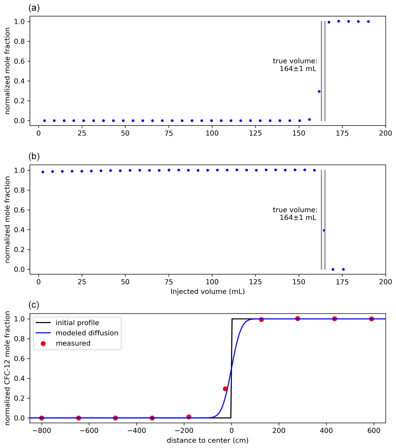
Figure 4 Results of StratoCore-GC-ECD flow-through tests from AirCore samples (showing CFC-12 as an example). (a): filling the AirCore with zero air, then analyzing the AirCore using StratoCore-GC-ECD with air with tropospheric mole fractions as the push gas. (b): filling the AirCore with tropospheric air, then analyzing the AirCore using StratoCore-GC-ECD with zero air as push gas. The grey lines in (a) and (b) represent the true volume of the test AirCore. (c): modeled diffusion at the AirCore gas–push gas boundary during AirCore analysis after 12 h.

The two tests also demonstrated limited mixing of the sample during the analysis. The push gas used in both tests differed from the gas in the AirCore, defining the transition between the AirCore sample and the push gas after each analysis. The measurements display sharp transitions from the sample to the push gas within 1–2 injections (<10 mL of air). These abrupt transitions indicate that due to the carefully controlled flow during the sample loading process and minimized pressure drop during valve switching, the sample mixing during the analysis is minimal. Here, we used a simple mixing model to estimate the molecular diffusion and Taylor dispersion between the push gas and the sample gas in the AirCore:

$$\begin{array}{}\text{(1)}& X_{\mathrm{rms}}=(\mathrm{2}\cdot D_{\mathrm{eff}}\cdot t{)}^{\mathrm{0.5}},\end{array}$$

in which X_rms is the root-mean-squared diffusion distance, t is time, and D_eff is an effective diffusivity incorporating both the molecular diffusion and the Taylor dispersion:

$$\begin{array}{}\text{(2)}& D_{\mathrm{eff}}=D+{\displaystyle \frac{a^{\mathrm{2}}{v}^{\mathrm{2}}}{\mathrm{48}D}}.\end{array}$$

In Eq. (2), D is the molecular diffusion coefficient, a is the tube radius, and v is the average air velocity. Using the equations, we modeled the diffusion between the push gas and the sample gas during the analysis period (∼ 1 h) for the test AirCore, shown in Fig. 4c. The modeled X_rms on the back end of the AirCore was 37.4 cm (equivalent to 2.5 mL of air), in line with the observed sharp transition between the push gas and the sample gas. Therefore, we suggest that the flow in the StratoCore-GC-ECD system during sample analysis remains a rigid “slug flow” moving through the system.

Additionally, the results from the two tests demonstrated high accuracy of volume registration by the StratoCore-GC-ECD system. Using the mass flow meter, we registered each data point to the volume of the AirCore. The measured volume of the AirCore by the StratoCore-GC-ECD system is defined as the midpoint of the transition between the AirCore gas and the push gas. In the meantime, we carefully measured the true volume of the AirCore multiple times by weighing the amount of water needed to fill the entire AirCore. The total volume of the AirCore measured by the StratoCore-GC-ECD system agrees with the actual volume of the AirCore within ± 1 mL, suggesting the volume measurements are accurate to within ± 0.6 %.

A final set of tests was also conducted to further verify that using a simple 1-D diffusion model, we can quantify the diffusion of the sample in the AirCore over a known storage time, and minimal mixing occurred during the sample loading process. The AirCore was filled with two alternating slugs using two calibrated dry standard gas cylinders. The two standards have different dry mole fractions of all the target molecules and CO₂, CO, and CH₄; therefore the transition between the two slugs can be observed using both a continuous analyzer that measures the CO₂ mole fraction and the StratoCore-GC-ECD. During the filling process, the transitions between slugs in the AirCore (Karion et al., 2010) were directly measured by a continuous gas analyzer (G2401, Picarro, CA, USA), shown as the varying CO₂ mole fractions in Fig. 5a. Subsequently, the AirCore was closed, quickly connected to the StratoCore-GC-ECD system, then analyzed immediately. The N₂O mole fractions show the transitions between slugs measured by the StratoCore-GC-ECD (Fig. 5a). The transitions observed by both the direct continuous measurements and the StratoCore-GC-ECD display good agreement, again suggesting mixing induced by StratoCore-GC-ECD's sample loading process is negligible. In addition, the AirCore was filled with two alternating slugs (the same as the previous test), then stored for 26 h before being analyzed by the StratoCore-GC-ECD. After the longer, 26 h storage, the StratoCore-GC-ECD measurements suggest that the mixing between slugs was significantly enhanced (Fig. 5b). Assuming a 1-D diffusion model along the length of the AirCore, we used Eq. (1) to model the molecular diffusion inside the AirCore during storage. The modeled diffusive mixing between slugs can capture the observed mixing well (Fig. 5b), suggesting that the horizontal mixing in the tubing coil during the storage time between AirCore landing and sample analysis can be calculated and accounted for in the calculation of the uncertainty of the AirCore altitude registration.

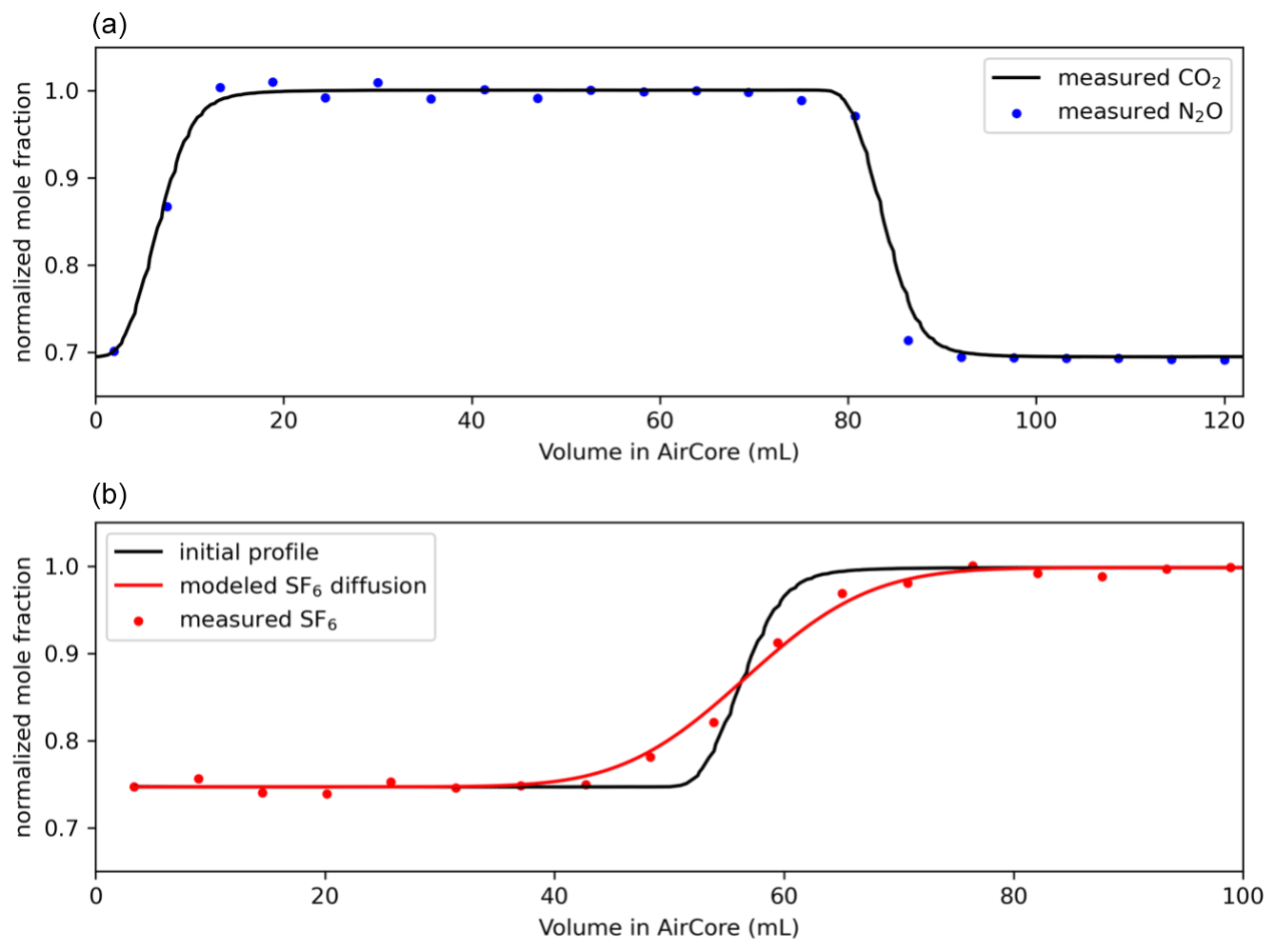
Figure 5 (a): results from the alternating-slug test. The AirCore was filled by two alternating slugs (with normalized CFC-11 dry mole fractions of 0.7 and 1, respectively), then immediately analyzed by StratoCore-GC-ECD. The black line represents the transition between two slugs measured by the continuous-flow analyzer; blue points are StratoCore-GC-ECD measurements. (b): results of the storage test using the same alternating slugs. The black line represents the transition between two slugs when the AirCore is being filled, the red line represents the modeled 1-D diffusion after 26 h storage, and the red dots are the measurements from the StratoCore-GC-ECD.

3 Balloon-borne AirCore flights

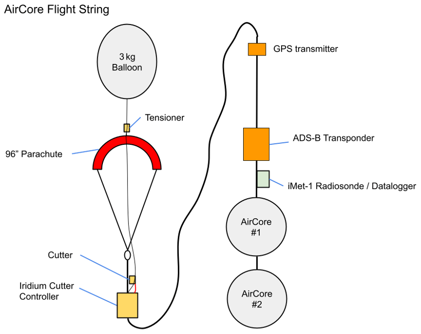
Four balloon-borne AirCore test flights were conducted to retrieve the vertical profiles of CFC-11, CFC-12, CFC-113, H-1211, N₂O, and SF₆ in the stratosphere. The balloons were launched in northeastern Colorado, USA, on 8 September 2021 (flight 1), 16 November 2021 (flight 2), 31 March 2022 (flight 3), and 9 August 2022 (flight 4). A 3000 g weather balloon filled with helium carried the flight train on each flight to ∼ 29.5 km a.m.s.l. The payload package in the test flights is identical to routine AirCore flights of the ongoing AirCore program at NOAA/GML (Fig. 6). Each package contains a parachute: a cutter that can be remotely controlled to release the balloon and open the parachute; a GPS transmitter for real-time tracking of the flight; an Automatic Dependent Surveillance–Broadcast (ADS–B) transponder; a radiosonde (InterMet systems iMet-1 RSB, MI, USA) for recording latitude, longitude, altitude, temperature, atmospheric pressure, and relative humidity; and two AirCores. The two AirCores used in each flight are identical to ensure the sampling processes of both AirCores are the same and confirm that there is no contamination to the AirCore samplers. In flights 1–3, the AirCores consisted of 91 m long tubing, with an outer diameter of 0.32 cm and inner diameter of 0.29 cm (total volume: 600 mL), with a valve placed on each end (top and bottom valves). The AirCores used in flight 4 (9 August 2022) were optimized for stratospheric air sampling (see discussion below) and consisted of two tubing segments: the tropospheric portion (open end when sampling) was a 21 m tube with an inner diameter of 0.58 cm, and the stratospheric portion was a 28 m tube with an inner diameter of 0.29 cm (740 mL total volume with approximately 25 % in the thinner tubing). Before the flight, each AirCore is insulated using a polymer foam package, wrapped with plastic wrap to minimize damage in the field, and covered by a custom-made bag using high-strength, lightweight Dyneema composite fabric. A data logger (Arduino, MA, USA) placed next to the AirCore inside the polymer foam recorded the coil temperature at multiple locations, latitude, longitude, altitude, and atmospheric pressure at 1 Hz.

Figure 6 Components of a typical NOAA AirCore flight train.

Hours before each flight, AirCores are flushed with special gases to distinguish between the residual fill gas not evacuated from the AirCore during flight and atmospheric samples during analysis. The AirCores used for CO₂, CH_4,, and CO measurements (by continuous analyzers) are flushed with an air mixture with a high CO dry mole fraction (1765 ppb) and known CO₂ and CH₄ dry mole fractions. The AirCores analyzed on the StratoCore-GC-ECD system are flushed with zero air, containing elevated H-1211 (6.6 ppt). We selected H-1211 as the tracer for the remaining fill gas because of the rapid photochemical destruction of H-1211 in the lower stratosphere: atmospheric models and in situ aircraft observations (Portmann et al., 1999; Papanastasiou et al., 2013; Moore et al., 2014; Elkins et al., 2020) showed H-1211 is entirely destroyed above 25 hPa (∼ 20–22 km a.m.s.l.). Since the topmost sampling altitude of our AirCore is higher than 25 km a.m.s.l., H-1211 is an ideal tracer for distinguishing the residual fill gas in the AirCore from air samples collected above 24–25 km a.m.s.l. After the AirCores are thoroughly flushed, the bottom valves are kept closed until minutes before the flight to minimize potential contamination from ambient air.

The flight trajectories of all four test flights are shown in Fig. 7. The balloon setup is designed such that the payload for all the flights should have similar ascent and descent processes: the balloon carries the payload to 28.9 km a.m.s.l. (10 hPa) at ∼ 6 m s⁻¹, then the cutter is activated to release the payload from the balloon. After the balloon cutaway, the parachute is deployed and the payload descends, during which the AirCores passively collect ambient air. One exception was flight 3: after the balloon cutaway, the parachute did not fully open, resulting in a faster descent rate. After landing, the bottom valve on the AirCore closes automatically after ∼ 30 s to minimize sample loss and potential contamination and loss of sample due to warming. The AirCores were quickly transferred back to the lab for analysis. In each flight, one of the AirCores was analyzed by a Picarro G2401 continuous gas analyzer for CO₂, CH₄, and CO dry mole fractions, and the other AirCore was analyzed by the StratoCore-GC-ECD (here, only the stratospheric portion (approximately the first 20 %–30 % of the AirCore) was analyzed). After the analysis, the filling process of the AirCore during descent is modeled using the meteorological data and a fluid dynamic program (Tans, 2022). The modeled results are then used to register the sample measurement time series with the altitude at which each sample was collected to derive the vertical profiles of all the trace gas measured by both instruments.

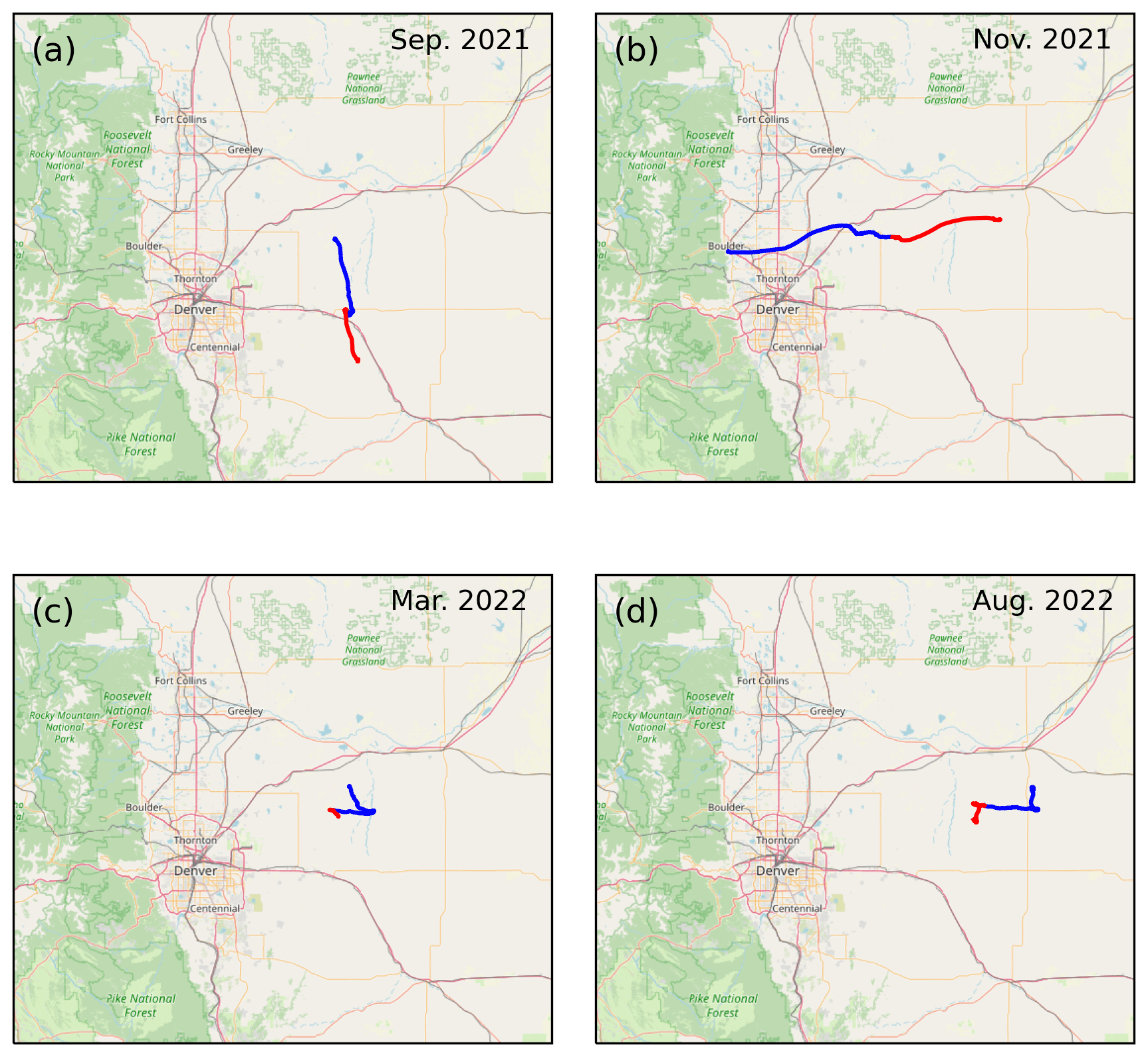
Figure 7 Flight trajectories of the four test flights in northeastern Colorado, USA. Panels (a)–(d) represent flights 1–4. The blue lines represent the payload ascent, and the red lines represent the descent. The base map is provided by ©OpenStreetMap contributors 2023. Distributed under the Open Data Commons Open Database License (ODbL) v1.0.

The AirCore dimensions have a significant impact on the sampling efficiency in the stratosphere (e.g., Membrive et al., 2017; Baier et al., 2023). The AirCores used in flight 4 had wider tubing (0.58 cm inside diameter) at the bottom (open end) and thinner tubing on top (0.29 cm inside diameter), while the AirCores used in flights 1–3 consisted of one piece of thin tubing (0.29 cm inside diameter). As a result, their sampling efficiencies in the stratosphere are drastically different. Using the fluid dynamic model described in Tans (2022), we modeled the outflow and inflow of AirCores during each flight, shown in Fig. 8. The model suggests that after the balloon cutaway, the volumetric inflow during flight 4 (Fig. 8a) increased much more rapidly compared to flights 1–3. The higher inflow in flight 4 is due to the larger diameter on the bottom portion of the AirCores used in flight 4, which produces a much smaller pressure gradient along the length of the tubing, making it easier for air to enter the sampler. Therefore, the stratospheric sampling efficiency, i.e., the ability of the AirCore to collect stratospheric air (Fig. 8b), of flight 4 was significantly higher than those of flights 1–3. The increased flow rates in flight 3 (compared to flights 1 and 2) were caused mainly by its fast descent, creating a large pressure gradient at the inlet of the AirCores. However, the combination of high flow rates and short descent time (60 % faster than other flights) in flight 3 still resulted in higher flow resistance in the AirCore, which reduced sampling efficiency. Indeed, the model shows that compared to the AirCores in flights 1 and 2, the AirCores in flight 4 are much closer to pressure equilibrium between the closed and open ends of the AirCore (Fig. 8c), while the AirCores in flight 3 displayed the most significant imbalance between open and closed ends during descent. This is demonstrated by the observed pressure differential between the open and closed ends of the AirCore: the pressure differential of the entire AirCore in every flight was measured at 1 Hz by a pressure transducer mounted on the closed end of the AirCore. Using the model output, we also calculated the overall pressure differential and compared it with the measurements. The modeled pressure differential (Fig. 8d) time series agrees with measurements in all the flights (data not shown in the figure): during the AirCore descent, the root-mean-square error (RMSE) between model output and measurements is less than 0.6 hPa (corresponding to approximately 240 m at 28 km a.m.s.l. and 20 m at 12 km a.m.s.l.), demonstrating that the model successfully reproduced the air sampling process. The AirCores used in flight 4 showed a much smaller pressure differential compared to the AirCores used in flights 1–3, highlighting the higher stratospheric sampling efficiency of the AirCore using modified tubing coil.

Figure 8 Modeled fluid dynamics of the AirCore filling process. Each line represents one flight, the dashed portion of each line represents the ascent, and the solid part represents the descent. (a): the modeled volumetric flow (in mL min⁻¹) into the AirCores during the entire flight, plotted against altitude; (b): the modeled mass flow (in µmol min⁻¹) into the AirCores; (c): the AirCore mass equilibrium ratio (actual air mass divided by equilibrium air mass in the AirCore) during the entire flight: a mass equilibrium ratio equal to 1 means the air inside the AirCore reaches equilibrium with ambient air, and a ratio lower than 1 means the air inside the AirCore is depleted and vice versa; (d): time series of the modeled pressure gradient across the entire AirCore.

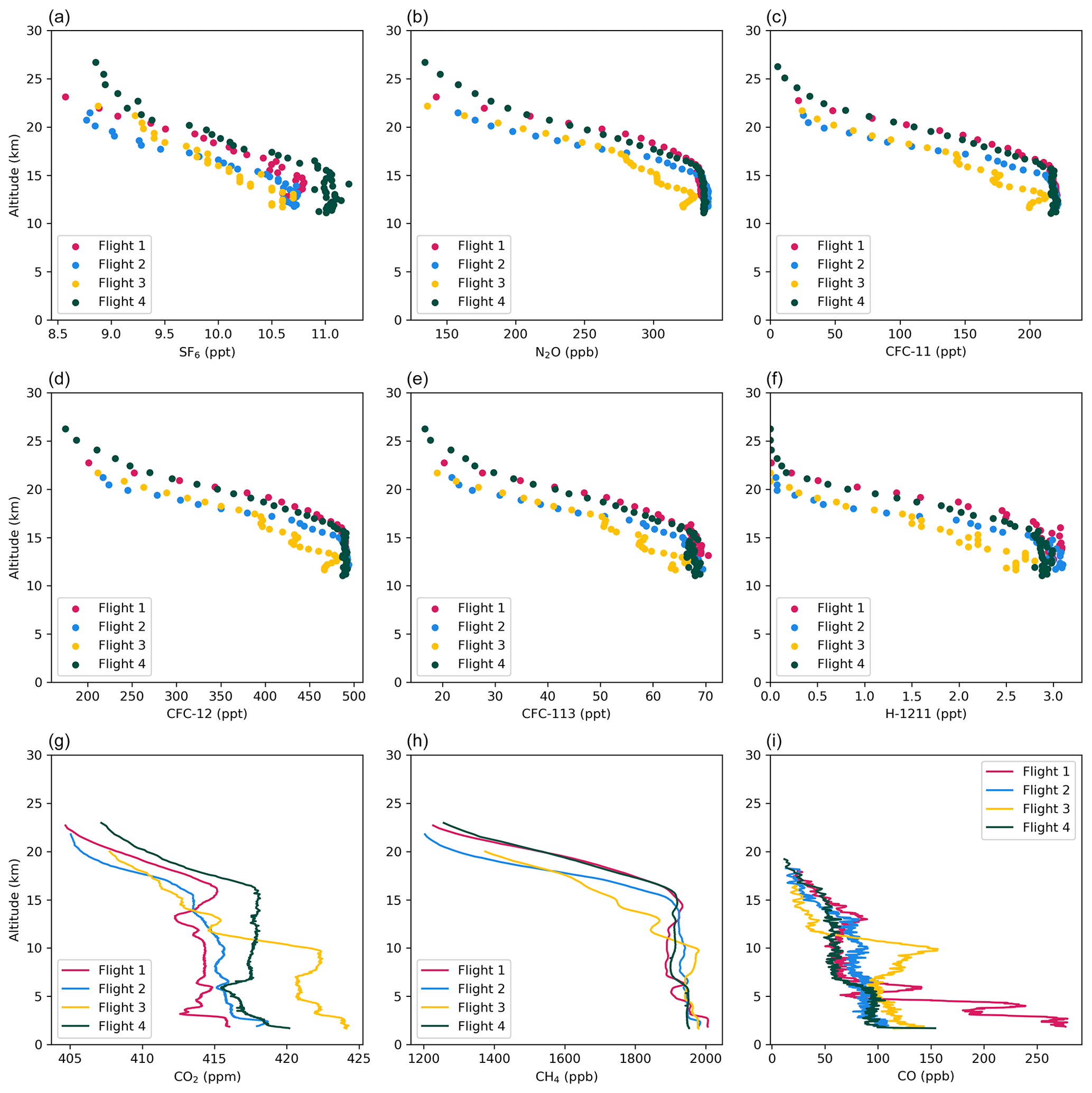
Figure 9 Vertical profiles of AirCore trace gas dry mole fractions measured from the four flights. Panels (a)–(f) are the results from the StratoCore-GC-ECD, from the tropopause to 25–28 km a.m.s.l. Each color represents one of the flights. Panels (g)–(i) are the mole fractions of CO₂ (g), CH₄ (h), and CO (i) analyzed by a Picarro G2401 continuous gas analyzer.

The StratoCore-GC-ECD analysis of AirCores from the four test flights yielded high-vertical-resolution profiles of target molecules, agreeing well with their predicted stratospheric photochemical loss processes. For all the target molecules measured by the StratoCore-GC-ECD system (Fig. 9a–f), analyzing the 600 mL AirCores (in flights 1–3) produces 31 to 38 stratospheric measurements from each AirCore, equivalent to one measurement every 5–7 hPa. The larger dual-diameter AirCore used in flight 4 yielded 50 measurements in the stratosphere with a resolution of 4.5 hPa per measurement (corresponding to approximately 1.6 km per measurement at 28 km a.m.s.l. and 0.14 km per measurement at 12 km a.m.s.l.). The decrease in dry mole fractions of the photolytic tracers with altitude can be explained by their stratospheric photochemical properties (Portmann et al., 1999; Moore et al., 2014): compared to mean tropospheric values, the average loss (in %) of each photolytic tracer at the 650 K isentrope (approximately 25 km a.m.s.l.) for the four test flights are 58 %±5 %, 61 %±4 %, 72 %±3 %, 93 %±3 %, and 100 % for N₂O, CFC-12, CFC-113, CFC-11, and H-1211, respectively. These values qualitatively agree with the relative stratospheric loss of the tracers via photolysis (e.g., Moore et al., 2013): at any given altitude in the stratosphere, the photolysis lifetimes of each molecule, from longest to shortest, are N₂O > CFC-12 > CFC-113 > CFC-11 > H-1211. In addition, the high-resolution analysis from the StratoCore-GC-ECD systems captured temporal stratospheric variability, such as the variable dry mole fractions of all molecules at 10–17 km in flight 3 (Fig. 9). Similar structures were also observed in the CO₂ and CH₄ profiles obtained from the continuous analyzers using the other AirCore on the same flight string (Fig. 9g, h). Therefore, the observed variability in the AirCore profiles is unlikely to originate from artifacts during the sampling or measurement processes but reflects short-term atmospheric conditions that may have developed from episodic stratospheric dynamic events. The observed variability, which is significantly larger than detection limits and calculated mixing in the AirCore, suggests that the StratoCore-GC-ECD system allows us to obtain high-vertical-resolution observations of the stratosphere.

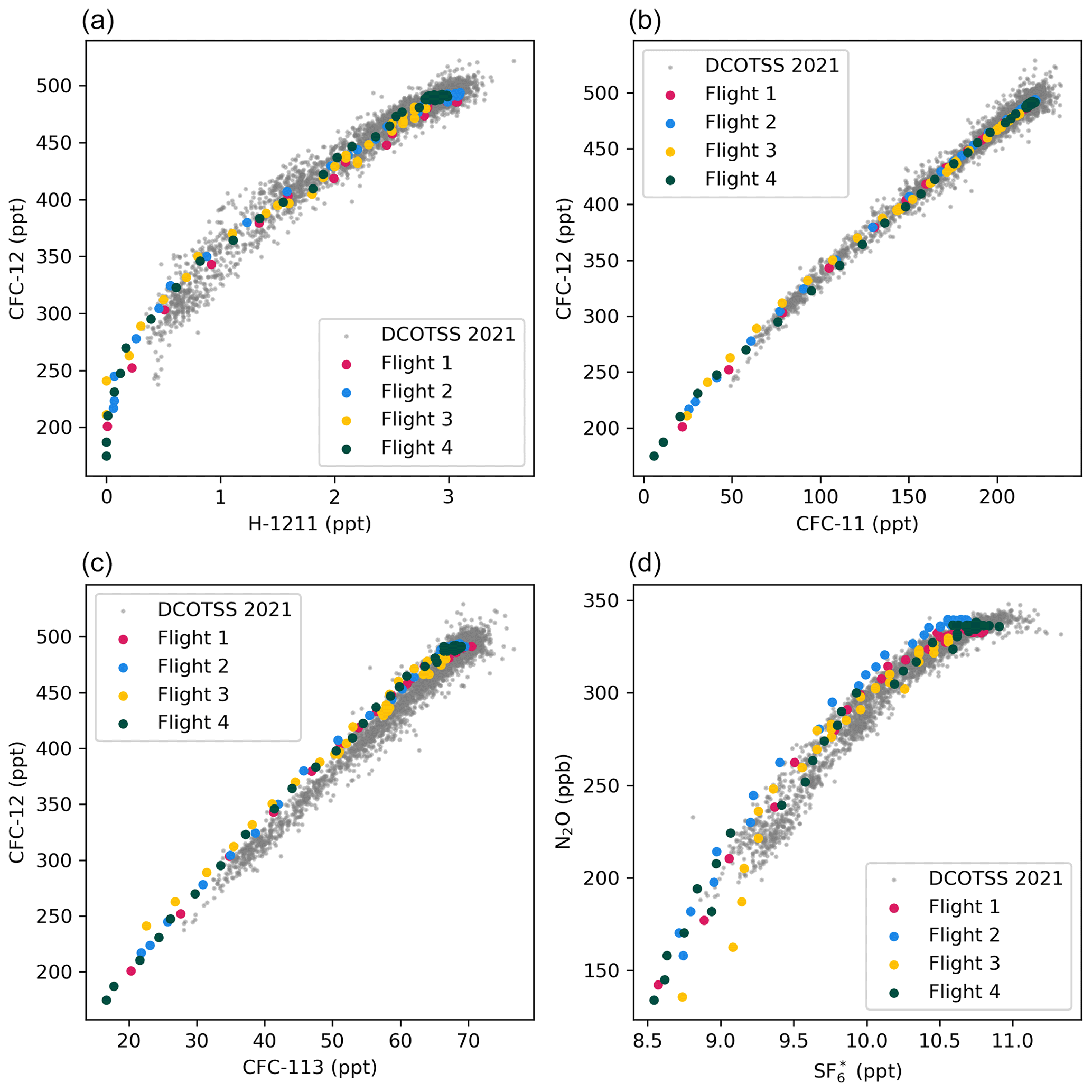
Figure 10 Relationships between different molecules measured by the StratoCore-GC-ECD for flights 1–4. Grey points are aircraft measurements acquired from the 2021 NASA DCOTSS campaign over the central USA and Canada. ^∗ AirCore SF₆ data in panel (d) were corrected (based on the global average growth rate of SF₆ in 2020–2021) to account for the growth of SF₆ in the atmosphere.

The tracer–tracer relationships in the profiles collected to date show agreement with in situ observations from previous flight campaigns within analytical uncertainties. The relationships between different trace gases are shown in Fig. 10 and compared with in situ aircraft measurements using the UAS Chromatograph for Atmospheric Trace Species (UCATS; Hintsa et al., 2021) during the NASA Dynamics and Chemistry of the Summer Stratosphere (DCOTSS) campaign in Kansas, USA, in July–August 2021. The AirCores collected samples from a higher altitude (25–28 km a.m.s.l.), where there is more aged air and more pronounced photolytic loss of trace gases compared to the ER-2 research aircraft (up to 21 km a.m.s.l.). The relationships between CFC-11, CFC-12, and H-1211 measured from AirCores agree with those of UCATS (Fig. 10a, b). For CFC-113, the StratoCore-GC-ECD measurements generally agree with UCATS measurements with a small but consistent (1–2 ppt) discrepancy (Fig. 10c). We speculate this discrepancy originates from different analytical methods used to calibrate working standards for the two measurements: the standards used in the UCATS measurement were calibrated using a GC-ECD. In contrast, the standards used in StratoCore-GC-ECD were calibrated using a GC-MS. A previous study showed a 1.3 ppt offset in CFC-113 measurements between a GC-ECD and a GC-MS (Rhoderick et al., 2015). It is possible that the observed discrepancy between StratoCore-GC-ECD and UCATS measurements reflected a similar offset. Further work is needed to understand the origin of this offset. SF₆ measurements from StratoCore-GC-ECD have been corrected to account for their growth in the troposphere using the global average growth rate of tropospheric SF₆ in 2021, and the corrected N₂O–SF₆ relationship also shows general agreement with UCATS data (Fig. 10d) with a small offset. We suggest that this small offset might originate from the uncertainty in estimating the tropospheric growth rate of SF₆. One exception is the uppermost AirCore samples in flight 3, which displays a slightly different N₂O–SF₆ relationship from the other three flights. We speculate that this might be due to the short-term stratospheric transport variability, which is most likely driven by a combination of seasonal changes in wave activity, quasi-biennial oscillation (QBO), El Niño–Southern Oscillation (ENSO), and other short-term, episodic events. Mapping this variation between AoA and photolytic-loss-dominated tracers allows us to investigate these drivers of stratospheric dynamics further but is outside the scope of this analysis. As we accumulate additional data in further flights, we can likely distinguish between these short-term variations and long-term changes driven by climate change.

4 Conclusions

The StratoCore-GC-ECD system, with a specially designed AirCore sample handling system (capable of injection of 4–5 mL of air for each analysis), can measure a suite of long-lived trace gases (N₂O, SF₆, CFC-11, CFC-12, H-1211, and CFC-113) from AirCore samplers with analytical precisions below 0.7 % for all gases. AirCore samplers designed with dimensions specially optimized for stratospheric sampling can obtain high-resolution vertical profiles of these trace gases from the tropopause to 28 km a.m.s.l. Four test AirCore flights were conducted in eastern Colorado from fall 2021 to summer 2022, with AirCores analyzed by the StratoCore-GC-ECD system. The results showed good agreement with model predictions and aircraft in situ measurements, suggesting that the StratoCore-GC-ECD system provides a robust, low-cost approach for observing the chemical composition of the stratosphere. In the future, this system will be applied for regular monitoring of the changes of these trace gases in the stratosphere, providing additional observational constraints on global climate models in a changing climate. We suggest that the sample handling system of the StratoCore-GC-ECD can be adapted to other analytical techniques to allow even more measurements (such as isotopic measurements) from AirCore samples in the future.