Detection of turbulence occurrences from temperature, pressure, and position measurements under superpressure balloons

This article deals with the detection of small-scale turbulence from in situ meteorological measurements performed under superpressure balloons (SPBs). These balloons allow long-duration flights (several months) at a prerequisite height level. The data set is gathered from the Strateole-2 probationary campaign during which eights SPBs flew in the tropical tropopause layer at altitudes of around 19 and 20.5 km from November 2019 to March 2020.

Turbulence is not directly measured by the instrument set onboard the SPBs. Nonetheless, there is the potential to derive information about the occurrence of turbulence from the temporally well-resolved measurements of pressure, temperature, and position. It constitutes a challenge to extract the aforementioned information from a measurement set that was not designed for quantifying turbulence, and the paper explains the methodology developed to overcome this difficulty.

It is observed that SPBs oscillate quasi-periodically around their equilibrium positions. The oscillation periods, which are 220 s on average with a range of 130 to 500 s, are close to but noticeably smaller than the Brunt–Väisälä period (∼300 s). The amplitude of these vertical motions is $\sim \pm \mathrm{15}$ m, inducing large fluctuations in all quantities, whether measured (e.g., pressure, temperature and position) or inferred (e.g., density and potential temperature). The relationships between the changes in these quantities and the vertical displacements of the balloons are used to infer properties of the flow in which the SPBs drift.

In the case of active turbulence, the vertical stratification as well as the wind shear are likely to be reduced by mixing. Hence, the increments of potential temperature, δθ, and of the vertical displacements of the balloon, δz_B, are expected to be uncorrelated because $\partial \mathit{\theta }/\partial z\to \mathrm{0}$. Moreover, the local vertical gradients of measured quantities, temperature (T) and horizontal velocities (u and v), are estimated from the covariance of the increments of the considered quantity with δz_B. The Richardson number of the flow is deduced.

Several binary indexes (true or false) to describe the state of the flow, laminar or turbulent, are evaluated. These turbulence indexes, based either on correlations between δθ and δz_B or on estimates of the local Richardson number, are found to be consistent, as they differ in less than 3 % of cases. The flow is observed to be turbulent for about 5 % of the time, with strong inhomogeneities along the longitude.

1 Introduction

The vertical transport of heat, momentum, and minor constituents in the tropical upper troposphere–lower stratosphere (UTLS) is an important issue, as this region is recognized as the gateway for tropospheric air into the stratosphere (Fueglistaler et al., 2009). Above 15 km altitude, this vertical transport is believed to mainly result either from the mean tropical upwelling associated with the Brewer–Dobson circulation or from small-scale turbulence. The relative contribution of turbulent mixing to this vertical transport is highly uncertain, partly owing to the lack of observations. Turbulence observations in the tropical UTLS are indeed sparse: they mostly come from two large very high frequency (VHF) radars, from relatively few radiosondes, or from research aircraft.

From measurements of the Equatorial Atmospheric Radar (EAR), located in West Sumatra (0.20^∘ S, 100.32^∘ E), Indonesia, Fujiwara et al. (2003) observed intermittent turbulence near the tropical tropopause with significant enhancements (a factor of 5) in the turbulent kinetic energy (TKE) lasting several days. Such enhancements in the TKE are believed to result from the breaking of large-scale Kelvin waves. Using the same EAR data set, Yamamoto et al. (2003) showed that eastward vertical wind shear around the equatorial tropopause frequently generates turbulence through Kelvin–Helmholtz instabilities (KHIs). Mega et al. (2010) presented detailed structures of KHIs in the equatorial UTLS from both high-resolution EAR measurements (using an interferometric imaging method) and radiosondes. From the VHF radar located in Gadanki (13.5^∘ N, 79.2^∘ E), India, Satheesan and Murthy (2002) and Satheesan and Krishna Murthy (2004) described turbulence characteristics in the tropical UTLS. These authors estimated TKE and TKE dissipation rates using several methods. Interestingly, they did not observe a clear variability in the turbulence intensity within the UTLS with altitude.

Sunilkumar et al. (2015) and Muhsin et al. (2016) presented the characteristics of turbulence in the tropical UTLS from GPS radiosonde observations obtained during more than 3 years at two stations located on the Indian Peninsula: Trivandrum (8.5^∘ N, 76.9^∘ E) and Gadanki (13.5^∘ N, 79.2^∘ E). The turbulent layers were detected using Thorpe's analysis (Thorpe, 1977) and following the procedure proposed by Wilson et al. (2010, 2011, 2013). The statistics of various turbulence parameters as well as the Brunt–Väisälä frequencies and the vertical shears are described for the convective troposphere and for the UTLS. The parameters describing the turbulence are either directly measured, such as the Thorpe lengths (an outer scale of turbulence) and the frequency of appearance of unstable layers, or are inferred on the basis of physical assumptions, like the TKE dissipation rates and the eddy diffusivity. Muhsin et al. (2020) extended the two previous studies by analyzing the soundings of six stations in South India, adding the Cochin (10^∘ N, 76.3^∘ E), Coimbatore (10.9^∘ N, 76.9^∘ E), Goa (15.5^∘ N, 73.8^∘ E), and Hyderabad (17.5^∘ N, 78.6^∘ E) stations to the two previously mentioned. These data were acquired during 4 years, from August 2013 to December 2017. All of these studies, based on radiosondes measurements, consistently show that the probability of occurrence of instability, either estimated from the gradient Richardson number (Ri) or from the squared Brunt–Väisälä frequency (N²), decreases with altitude above an altitude of 15 km, i.e., in the UTLS. They found that the probability of occurrence for Ri to be less than 0.25 is between 0 % and 5 % in the height range from 18 to 25 km and that the probability of occurrence of unstable regions (N²<0) is quasi-null. Interestingly, Muhsin et al. (2016) did not observe a clear diurnal cycle in the tropical UTLS.

Many studies of turbulence in the free atmosphere have been based on measurements from research aircraft (see Dörnbrack et al., 2022, and references therein); however, to our knowledge, only one study has involved the tropical UTLS. Podglajen et al. (2017) used high-resolution (20 Hz) airborne measurements to study the occurrence and properties of small-scale (≲100 m) wind and temperature fluctuations in the tropical UTLS over the Pacific Ocean. They showed that wind fluctuations are very intermittent and appear to be localized in shallow layers, typically with ∼100 m thickness. Furthermore, active turbulent events appear to be more frequent at relatively low altitude and near deep convection. They observed that the motions are close to 3D isotropic and that the power spectra follow a $\sim -\mathrm{5}/\mathrm{3}$ power law scaling. The diffusivity induced by turbulent bursts is estimated to be in the order of 10⁻¹ m² s⁻¹ and decreases from the bottom to the top of the tropical UTLS.

Apart from convective regions, many observations of the free atmosphere show successions of strata, i.e., alternating layers in which the flow is turbulent, whose depth varies from a few tens to a few hundreds of meters, separated by stable static regions, i.e., regions where the flow is laminar (e.g., Luce et al., 2015; Podglajen et al., 2017; Wilson et al., 2018). The numerical simulations of Fritts et al. (2003) support such observations. Turbulent and laminar strata are expected to exist in the tropical UTLS. As turbulence, by nature, is a dissipative process, the turbulent layers have a finite lifetime, depending on the mesoscale processes yielding energy (shear instability or wave breaking). Thus, by observing the flow at a given altitude level, we expect to find an alternation of turbulent and laminar episodes.

The Strateole-2 project has been set up in recent years in order to better understand the dynamics, transport, microphysics, and dehydration of the tropical UTLS (Haase et al., 2018). It is an international project involving several research groups, mostly in France and the USA, led by the Laboratoire de Météorologie Dynamique (LMD) and Centre National d'Études Spatiales (the French space agency). The uniqueness and strength of the Strateole-2 project come from the fact that the atmospheric measurements are obtained under superpressure balloons (SPBs) that can fly for several months (typically 3 months) at an approximately constant density level. Standard measurements performed under all of the Strateole-2 SPBs, including temperature, pressure, and GPS position, allow one to describe meso- and small-scale dynamic processes at the flight level, in a quasi-Lagrangian way (Hertzog and Vial, 2001; Hertzog et al., 2012; Podglajen et al., 2016; Corcos et al., 2021). The SPBs usually carry a second gondola with several configurations of instruments, allowing measurements of constituents, aerosols, cloud heights, and radiation, among others.

The main purpose of this paper is to present the methods allowing one to determine the dynamical state of the flow, laminar or turbulent, in which the SPBs are flowing. It is based on the estimation of the local stratification of the flow using measurements of temperature, pressure, and GPS position. The rest of the paper is organized as follows: the data set used is presented in Sect. 2, the methods for detecting turbulence and for estimating various indicators of the flow stability are described in Sect. 3, some results are presented (Sect. 4) and discussed (Sect. 5), and a concluding section (Sect. 6) summarizes the main findings of the paper.

2 The data set

2.1 The Strateole-2 C0 campaign

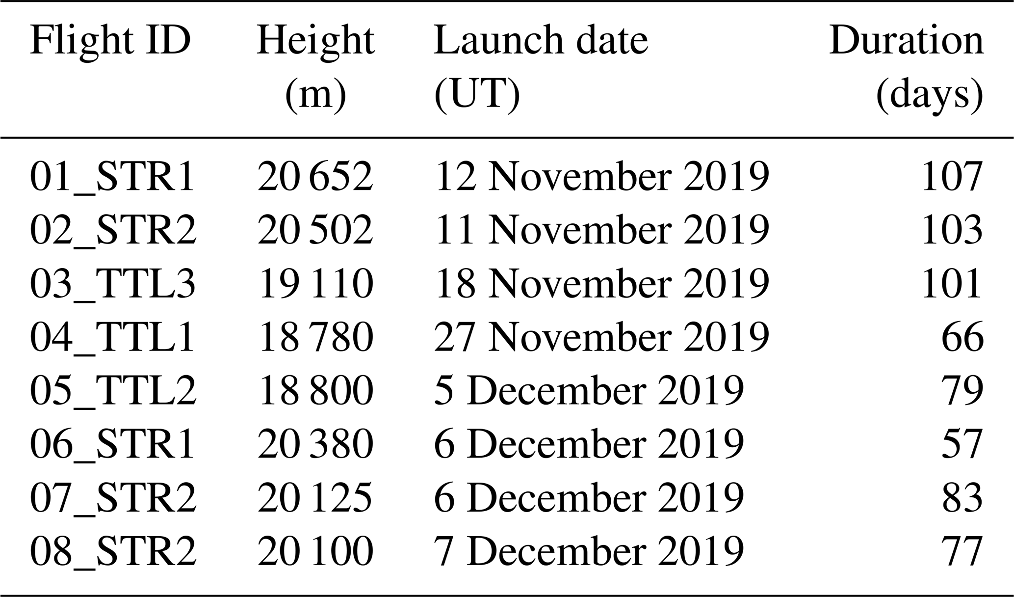
The probatory Strateole-2 campaign, called Strateole-2 C0, was held from November 2019 to March 2020. During this campaign, eight SPBs were launched from Mahé (4^∘37^′ S, 55^∘27^′ E), Seychelles, and flew eastward following the quasi-biennial oscillation (QBO) phase that prevailed in the lower stratosphere at this time (Fig. 1). The main characteristics of the flights are provided in Table 1. Four of these flights carried only the TSEN (Thermodynamics SENsors) instrument and its associated GPS receiver, whereas the other four carried additional scientific instruments. At first order, SPBs fly at a quasi-constant density level (Vincent and Hertzog, 2014). TTL and STR flights were associated with different carried masses and/or balloon sizes, and they drifted at altitudes of ∼19 and ∼20.5 km, respectively.

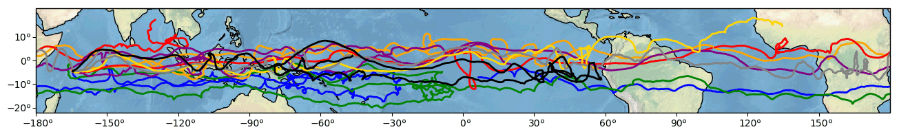
Figure 1 Trajectories of the eight SPBs.

Table 1 Main characteristics of Strateole-2 C0 flights. All superpressure balloons are equipped with TSEN (Thermodynamics SENsors) instruments.

2.2 The TSEN measurements

In this study, we use the TSEN measurements that are performed at the balloon flight level for each flight. They consist of two respective temperature measurements, one with a thermistor sensor (T_S) and one with a thermocouple sensor (T_C), and a pressure measurement (P). They are closely associated with GPS observations that provide the position (long; lat; and altitude above sea level, a.s.l.) of the balloon as well as with the solar zenith angle (SZA). All of these measurements are acquired every 30 s, except for the pressure measurements that are acquired every 1 s.

These raw measurements enable us to compute two estimates of the balloon potential temperature (θ_S and θ_C) and density (ρ_S and ρ_C), respectively, obtained with the thermistor and thermocouple temperatures. The horizontal velocity components (u and v) are evaluated from successive GPS positions.

In the following, we will make use of the increments of measured quantities, namely the differences between consecutive measurements: δT_S will, for instance, stand for the increments of the thermistor temperatures. Note that two independent estimates of the balloon vertical displacements are available: (1) δz_GPS obtained with the raw GPS altitudes and (2) δz_P computed with the pressure measurements and further assuming hydrostaticity.

TSEN measurements were also performed on the profiling unit of the Reeldown Aerosol Cloud Humidity and Temperature Sensors (RACHuTS) instrument (Kalnajs et al., 2021). RACHuTS notably allows one to obtain vertical temperature profiles of 2 km length below the balloon by reeling down (and then up) the profiling unit at a vertical velocity of about 1 m s⁻¹. Only one TSEN temperature sensor (a thermistor) is implemented in the profiling unit. Measurements are performed with a nominal sampling rate of 1 Hz, i.e., the vertical resolution of the RACHuTS temperature profiles is ∼1 m. We degraded its vertical resolution to about 30 m in order to (1) improve upon the 1 m raw precision of altitude measurements and (2) obtain a similar vertical resolution from TSEN and RACHuTS measurements (as the amplitude of the balloon oscillations is typically ±15 m).

Instrumental noise

The instrumental noise of the TSEN measurements is an important characteristic that has to be taken into account to assess whether the flow is turbulent. It is assumed that this noise is a zero-mean, uncorrelated process, i.e., a white noise, contributing to the measured signal. A way to estimate the white noise level is to compute the variance of the nth-order increments of the time series (n⪆6), such as high-order differentiation performing a high-pass filtering of the time series. As shown in Appendix A, the variance of the nth-order increments tends to the variance of the uncorrelated signal weighted by the sum of the squared binomial coefficients of order n−1. Here, noise levels are estimated on time segments of 21 samples (10 min); thus, they are estimated on more than 10 000 segments for a flight lasting ∼100 d. This method works well if the signal spectra exhibit a quasi-constant floor, i.e., if white noise clearly contributes to the measured signal for frequencies smaller than the Nyquist frequency, as is frequently the case for lidar or radar signals. However, we do not observe any white noise level for the TSEN measurements acquired with a sampling period of 30 s (T_S, z, u) (see, for instance, the power spectra of the vertical displacements δz shown in Fig. 6). Therefore, the variance of the nth-order increments cannot be interpreted as being solely due to uncorrelated noise, even if some noise is expected to contribute to this high-frequency variance. However, a rough estimate of the noise level has been evaluated from the data segments showing the smallest variances, i.e., segments for which a comparatively smaller contribution of the atmospheric signal is expected. Tables 2 and 3 display estimates of the noise levels for quantities measured or inferred, obtained with the average of the smallest 10 % of variance values of the sixth-order increments. Such estimates, although not fully satisfying, nevertheless provide valuable information on the relative quality of the data, allowing one to compare noise levels between sensors, between flights, or between night and day measurements.

Table 2 Estimated noise (standard deviation) of temperature, pressure, and dry potential temperature. For each flight, the first row indicates the flight-mean values (bold), and the second row indicates the respective nighttime and daytime average values.

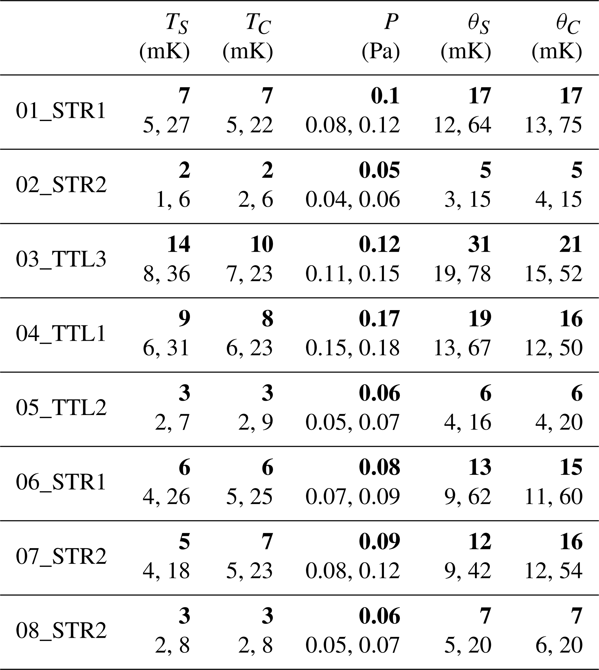
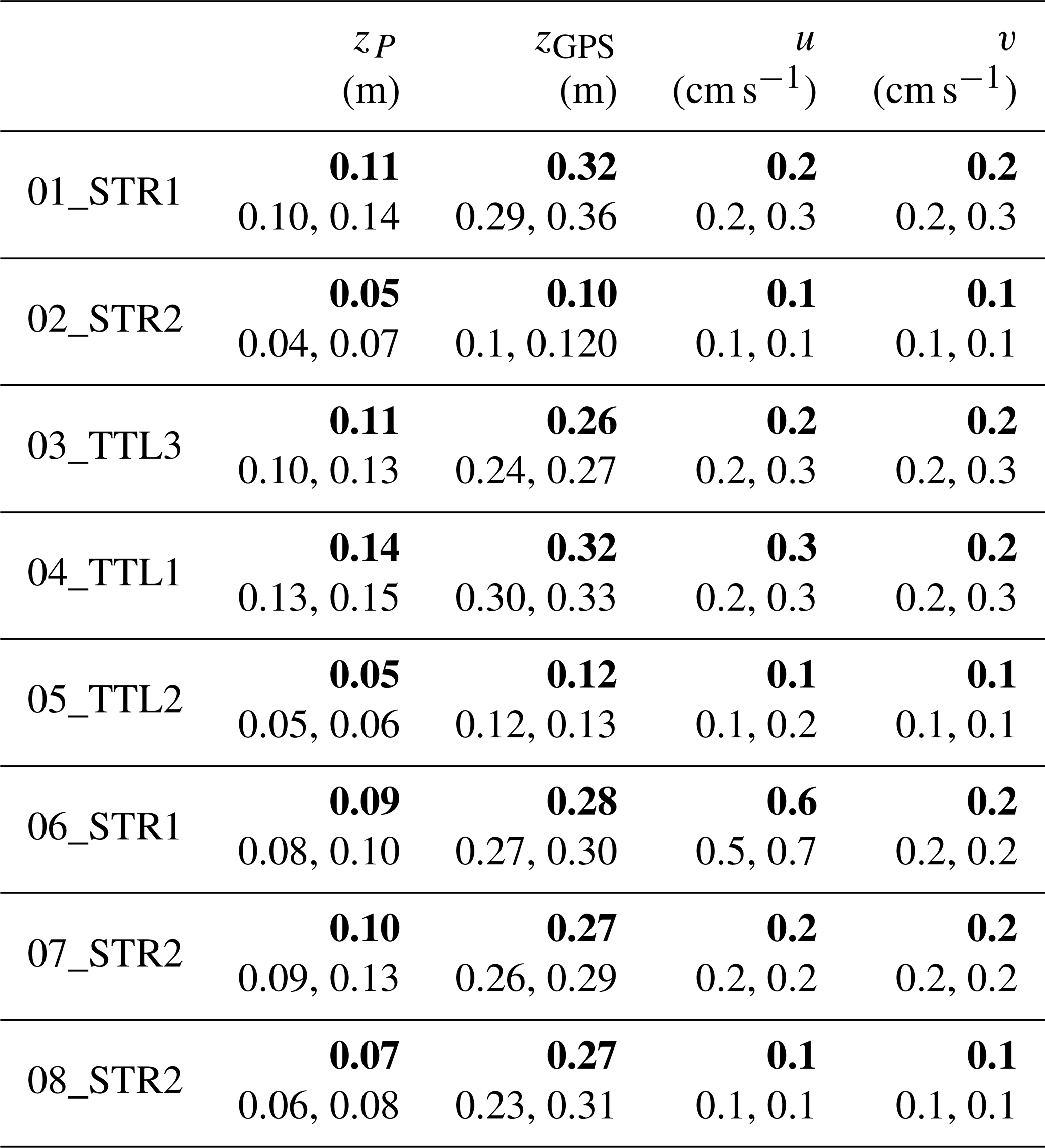
Table 3 Same as Table 2 but for altitudes derived from the pressure and altitude observations as well as zonal and meridional velocities.

The noise levels of the two temperature sensors, the thermocouple and thermistor, are quasi-identical. We note that the noise level of temperature measurements is a factor of 3–5 larger during daytime than during nighttime for all flights. Such an increase in temperature noise during the day very likely results from the random passage of the sensors in the wake of their electrical wires or mechanical support. These devices, which are significantly thicker than the sensors themselves, are heated by solar radiation during daytime and are consequently warmer than the air or even the sensor temperature. We also observe that the flight 03_TTL3 temperature measurements are the noisiest (14 mK vs. 2–9 mK). Unlike the other flights, during which temperature sensors were hanging at the very bottom of the flight train as far as possible from large elements (e.g., the gondolas), sensors on flight 03_TTL3 were located within the flight train. Thus, they were more prone to be affected by the warm wake of other devices in the flight train during daytime.

The noise estimates with respect to the pressure measurements and to the vertical position measurements (from both pressure differences and GPS) are slightly larger during daytime than during nighttime. The reason for this slight increase in the noise level is probably not the consequence of an increase in instrumental noise. It may rather be the consequence of the greater amplitudes of the balloon oscillations during daytime, which would impact the energy density of P and z at high frequency. The noise levels of the horizontal wind components estimated from GPS positions are very small, less than 1 cm s⁻¹. They do not show any night–day difference.

2.3 Oscillating movements of the balloons around their equilibrium positions

Superpressure balloons drift with the winds, following a quasi-Lagrangian behavior, which is useful to document the detailed evolution of a given air mass. Their displacements, however, differ from those of an air parcel in at least two ways. First and most importantly, the balloons follow isopycnic trajectories. The balloon envelope is almost inextensible, with the balloon diameter varying by less than 1 %; hence, the volume is fixed as long as a superpressure is present. As the total mass of the flight train is fixed, the density of the balloon remains constant, implying an isopycnic trajectory. In contrast, air parcels follow isentropic trajectories in the absence of diabatic forcing. The second difference comes from the existence of natural oscillations of the balloon around its equilibrium density surface (EDS), where it achieves neutral buoyancy. These oscillations are of minor importance for the study of phenomena on timescales larger than a few tens of minutes (Vincent and Hertzog, 2014). However, they will be central to the current study, as an oscillating balloon samples short vertical profiles of key meteorological variables. The methodology developed in the present study precisely aims at exploiting these short “unintended” vertical profiles to diagnose the occurrence of turbulence.

The atmospheric density (ρ) at the flight level is estimated from the measurements of temperature (T) and pressure (P) using the ideal gas law: $\mathit{\rho }=P/R_{\mathrm{a}}T$, where R_a is the ideal gas constant for dry air per unit mass. As two independent measurements of T exist, two estimates of ρ can be calculated, denoted as ρ_S and ρ_C, using the thermistor or thermocouple temperatures, respectively. Figure 2 displays the systematic balloon fluctuations in density about their EDS (Fig. 2a), as well as the related variations in balloon altitudes (Fig. 2b) during 4 h of flight 01_STR1. The fluctuations in density are about $\pm \mathrm{5}\times {\mathrm{10}}^{-\mathrm{4}}$ kg m⁻³, corresponding to relative fluctuations of $\sim \pm \mathrm{0.5}$ %. The corresponding amplitude of the balloon vertical displacements is ±20 m in this case. Thus, SPBs move around their EDS, exploring the atmosphere a few tens of meters above and below their position. These oscillatory motions induce fluctuations in the measured (P, T, z_GPS) and inferred quantities (ρ, θ, z_P). We shall use these variations to describe some properties of the flow by hypothesizing that the observed variability in a quantity depends on both the balloon vertical displacement and the local vertical gradient in the quantity.

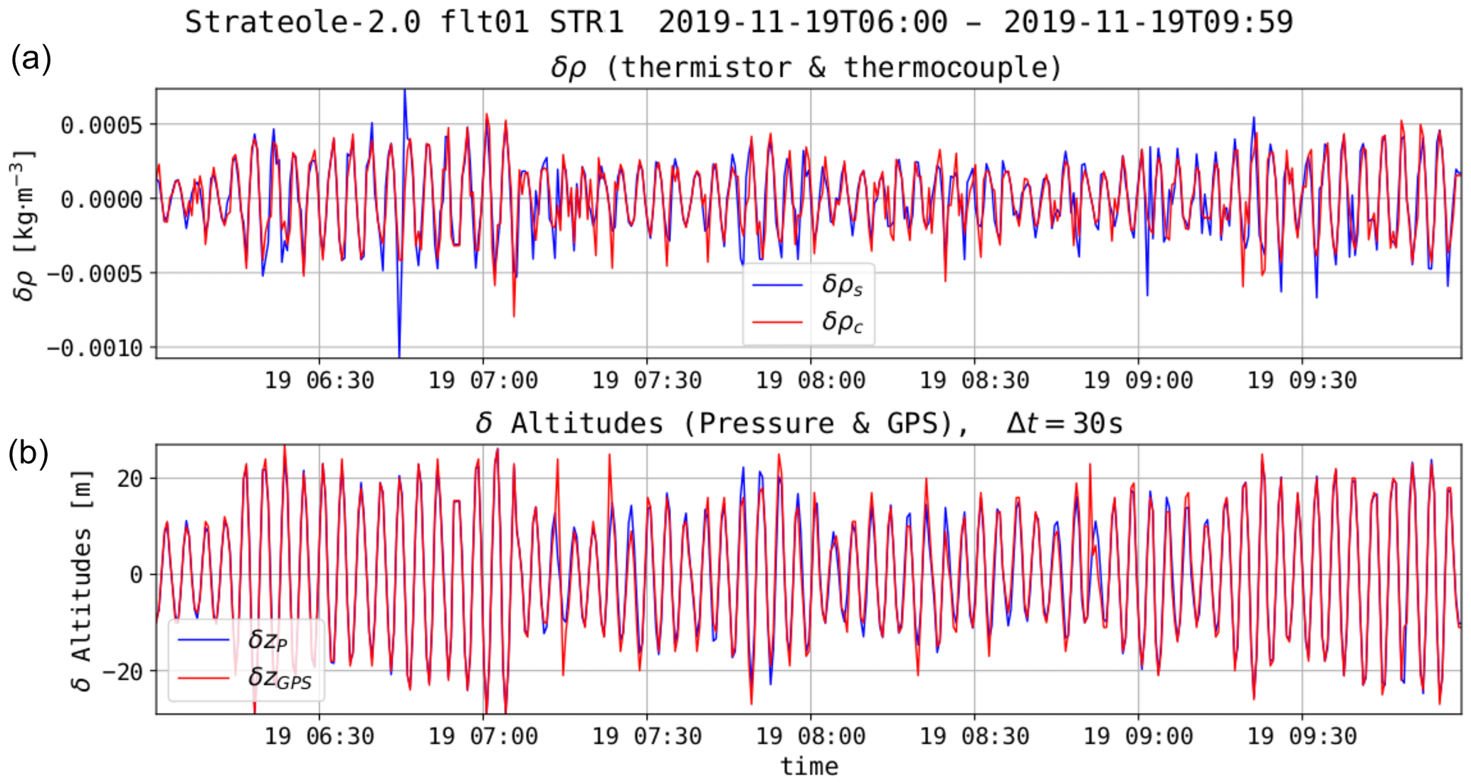
Figure 2 (a) Density fluctuations observed from 06:00 to 10:00 UTC on 19 November. (b) Fluctuations in the height of the balloon for the same time interval.

Periods and amplitudes of the vertical oscillations

Three angular frequencies, which are close to each other, first need to be distinguished: the Brunt–Väisälä frequency (N), the neutral buoyant oscillation frequency (ω_NBO), and the observed frequency of SPB oscillations (ω_B). The frequency at which a spherical balloon with constant volume oscillates about its EDS, the neutral buoyant oscillation (NBO) frequency, reads as follows (Hanna and Hoecker, 1971; Nastrom, 1980; Vincent and Hertzog, 2014):

$$\begin{array}{}\text{(1)}& {\mathit{\omega }}_{\mathrm{NBO}}^{\mathrm{2}}={\displaystyle \frac{\mathrm{4}{\mathit{\pi }}^{\mathrm{2}}}{t_{\mathrm{NBO}}^{\mathrm{2}}}}={\displaystyle \frac{\mathrm{2}g}{\mathrm{3}T}}\left({\displaystyle \frac{\partial T}{\partial z}}+{\displaystyle \frac{g}{R_{\mathrm{a}}}}\right),\end{array}$$

where t_NBO is the NBO period, and g is the acceleration of gravity. The squared Brunt–Väisälä (BV) frequency, $N^{\mathrm{2}}=g/T(\partial T/\partial z+g/c_p)$, can be expressed as a function of ${\mathit{\omega }}_{\mathrm{NBO}}^{\mathrm{2}}$:

$$\begin{array}{}\text{(2)}& N^{\mathrm{2}}={\displaystyle \frac{\mathrm{3}}{\mathrm{2}}}{\mathit{\omega }}_{\mathrm{NBO}}^{\mathrm{2}}-{\displaystyle \frac{g}{\mathit{\gamma }H}}={\displaystyle \frac{\mathrm{3}}{\mathrm{2}}}{\mathit{\omega }}_{\mathrm{NBO}}^{\mathrm{2}}-{\displaystyle \frac{\mathrm{5}}{\mathrm{7}}}{\displaystyle \frac{g}{H}},\end{array}$$

where c_p is the air specific heat capacity at constant pressure, γ is the heat capacity ratio, and $H=R_{\mathrm{a}}T/g$ is the atmospheric scale height.

From Eq. (2), it can be shown that N≤ω_NBO as long as ${\mathit{\omega }}_{\mathrm{NBO}}^{\mathrm{2}}\le \mathrm{10}g/\mathrm{7}H$, i.e., $t_{\mathrm{NBO}}\ge \mathrm{2.8}{\mathit{\pi }}^{\mathrm{2}}H/g\approx \mathrm{120}$ s, or $\partial T/\partial z\le \mathrm{8}g/\mathrm{7}{R}_{\mathrm{a}}\approx \mathrm{39}$ K km⁻¹. Such conditions are met very frequently in the lower stratosphere, if not always. Note that both ω_NBO and N increase with the vertical gradient of temperature $\partial T/\partial z$.

Figure 3a displays the observed periods of the balloon vertical oscillations (t_B) for the whole 01_STR1 flight. The gray and white stripes correspond to nights and days, respectively, and the orange curve shows the daytime and nighttime averages. The histogram of the oscillation periods is shown in Fig. 3b, and the periods are observed to range from ∼135 to 800 s. No clear day–night variation is visible. Figure 3c shows the cumulative distribution function (CDF) of the periods: the median t_B value is close to 220 s, and the mean is ∼250 s. Hence, ω_B is larger than N as long as N is smaller than $\approx \mathrm{2.5}\times {\mathrm{10}}^{-\mathrm{2}}$ rad s⁻¹, which is a typical value in the tropical lower stratosphere. In the following, we shall see that ω_B is systematically larger than N.

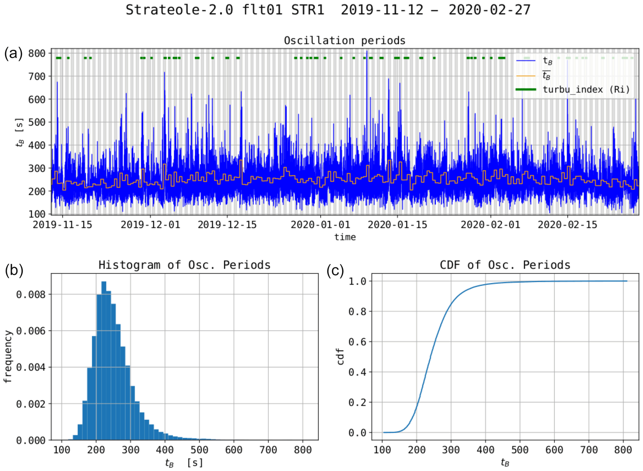
Figure 3 (a) Estimates of the SPB oscillation periods during flight 01_STR1; the orange staircase curve shows daytime and nighttime averages. (b) Histogram of the oscillation periods. (c) Cumulative distribution function of the oscillation periods.

Figure 4 shows the corresponding amplitudes of the observed balloon oscillations as well as their probability and cumulative distribution function. The observed amplitudes range from ∼0 to 150 m, with an average (median) of 14 m (15 m). Some large amplitude oscillations (>100 m) are observed. We found that they are most often associated with depressurization events. A weak but clear day–night variability is found: the oscillation amplitudes are about 20 % larger during daytime than during nighttime. Moreover, greater variability in altitude is observed during daytime at high frequencies, as reported in Table 3.

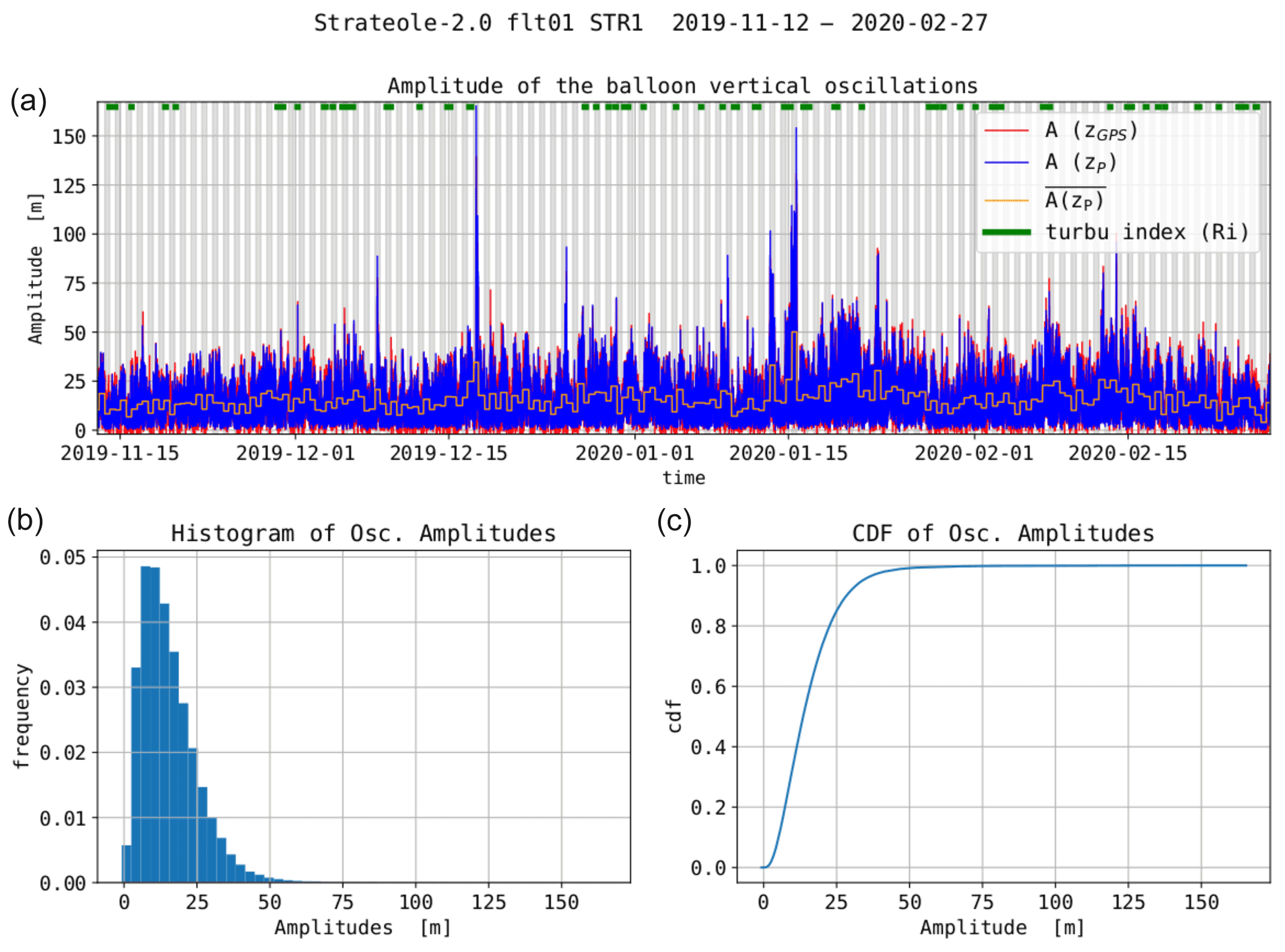
Figure 4 (a) Estimates of SPB oscillation amplitudes during flight 01_STR1; the orange staircase curve shows daytime and nighttime averages. (b) Histogram of the oscillation amplitudes. (c) CDF of the oscillation amplitudes.

3 Data processing

3.1 Methods for detecting the occurrence of turbulence from the TSEN measurements

The timescales of the turbulent fluctuations are expected to be smaller than the Brunt–Väisälä period, t_N. (In the following, “high frequencies” refer to frequencies larger than $N/\left(\mathrm{2}\mathit{\pi }\right)$.) As t_B is close to or even smaller than t_N, the high-frequency variability up to the Nyquist frequency ($\mathrm{1}/\mathrm{60}$ Hz) will be dramatically affected by the balloon oscillations regardless of the state of the flow (laminar or turbulent). Hence, the detection of turbulence from either the variance or the spectral characteristics of the TSEN measurements at high frequencies appears difficult, if not impossible.

Diagnostics on the dynamical state of the flow can, therefore, only be based on the local properties of atmospheric stratification, either stable or neutral/unstable. A consequence of turbulence is to restore stability from a preceding unstable state of the flow, which is achieved by locally mixing the fluid. In this case, the conservative quantities (potential temperature, specific humidity, and momentum) are expected to exhibit weak horizontal and vertical variability within the turbulent layer. Note that neutral or even unstable stratification conditions may precede turbulence, but such conditions cannot persist and will necessarily cause turbulence. Conversely, laminar flow is expected to exhibit significant variability in the same quantities along the vertical direction.

The first way to diagnose that the flow is turbulent is, thus, to detect a null gradient in potential temperature. In such a case, the correlation between the vertical displacements (δz_B) and the corresponding potential temperature increments (δθ) is expected to be null. Therefore, the implementation consists of testing the H₀ hypothesis of a null correlation between δz_B and δθ. This method is hereafter called the correlation method. The second way to diagnose a turbulent flow is based on the estimation of the local Richardson number $\mathit{Ri}=N^{\mathrm{2}}/S^{\mathrm{2}}$, where $S^{\mathrm{2}}=(\partial u/\partial z{)}^{\mathrm{2}}+(\partial v/\partial z{)}^{\mathrm{2}}$ is the squared shear. The flow is assumed to be turbulent when the Richardson number becomes less that 0.25. This method is hereafter called the Ri method.

3.2 Implementation of the two methods of turbulence detection

3.2.1 Relationship between the increments of measured quantities and the increments of vertical displacements

The two proposed methods of turbulence detection are based on either estimates of correlations (for the correlation method) or linear regressions (for the Richardson method) between increments. The increments are simply defined as the differences between consecutive measures, separated by δt=30 s. Such a differentiation realizes a high-pass filtering of the time series. Both the correlations and the linear regressions are computed over time periods of 1 h, i.e., with 120 observations that are 30 s long. The choice of this number of observations enables one to obtain relatively small uncertainties on the estimates of correlation coefficients and slopes, at the price of being unable to detect turbulence layers with timescales significantly shorter than 1 h (in the frame moving with the wind).

The oscillatory motions of SPBs at frequency ω_B are not expected to occur on isentropic surfaces nor on isopycnic surfaces. If the vertical displacement of the balloon between two different times separated by δt=30 s is $\mathit{\delta }{z}_{\mathrm{B}}=z_{\mathrm{2}}-z_{\mathrm{1}}$, the change in the measured potential temperature δθ depends on both δz_B and the vertical displacement of the atmosphere δζ_θ during δt:

$$\begin{array}{}\text{(3)}& \mathit{\delta }\mathit{\theta }=\stackrel{\mathrm{‾}}{{\mathit{\theta }}_z}(z_{\mathrm{2}}-z_{\mathrm{1}}^{\prime })=\stackrel{\mathrm{‾}}{{\mathit{\theta }}_z}(\mathit{\delta }{z}_{\mathrm{B}}-\mathit{\delta }{\mathit{\zeta }}_{\mathit{\theta }}),\end{array}$$

with $\mathit{\delta }{\mathit{\zeta }}_{\mathit{\theta }}=z_{\mathrm{1}}^{\prime }-z_{\mathrm{1}}$ corresponding to the change in the height of the isentropic surface during δt (see Fig 5). Equation (3) must be modified for nonconservative quantities, such as temperature (T) or horizontal velocities (u and v), in order to take into account the change in the considered quantity during δt on the isentropic surface. For instance, the temperature increment reads as follows:

$$\begin{array}{}\text{(4)}& \mathit{\delta }T=\stackrel{\mathrm{‾}}{T_z}\mathit{\delta }{z}_{\mathrm{B}}-\left(\stackrel{\mathrm{‾}}{T_z}+{\displaystyle \frac{g}{c_p}}\right)\mathit{\delta }{\mathit{\zeta }}_{\mathit{\theta }}.\end{array}$$

Figure 6 shows the power spectral density (PSD) of the vertical displacements (δz_B) for flight 02_STR2, either estimated from the GPS altitudes (δz_GPS) or from the pressure observations (δz_P). Both PSDs look very similar over the whole frequency range. A large spectral peak, centered at $\sim \mathrm{4}\times {\mathrm{10}}^{-\mathrm{3}}$ Hz, is observed on these PSDs. This spectral peak corresponds to the SPB oscillatory motions about their EDS with a period of ∼220 s, as described in Sect. 2.3. Apart from long-duration balloons, radar is one of the few techniques that is able to infer the air vertical velocity in the free atmosphere. Few radar-borne PSDs of the vertical velocity have been published (Ecklund et al., 1986; VanZandt et al., 1991; Satheesan and Murthy, 2002). They either show a weak enhancement at frequencies close to N with respect to the spectral level at ω≲N or no enhancement at all. Thus, it is believed that the high-frequency vertical displacements in the balloon observations, 15 m on average, mostly result from the balloons' oscillating motions about their EDS, rather than from the isentropic vertical displacements of air parcels. In other words, δz_B≫δζ_θ in Eqs. (3) and (4).

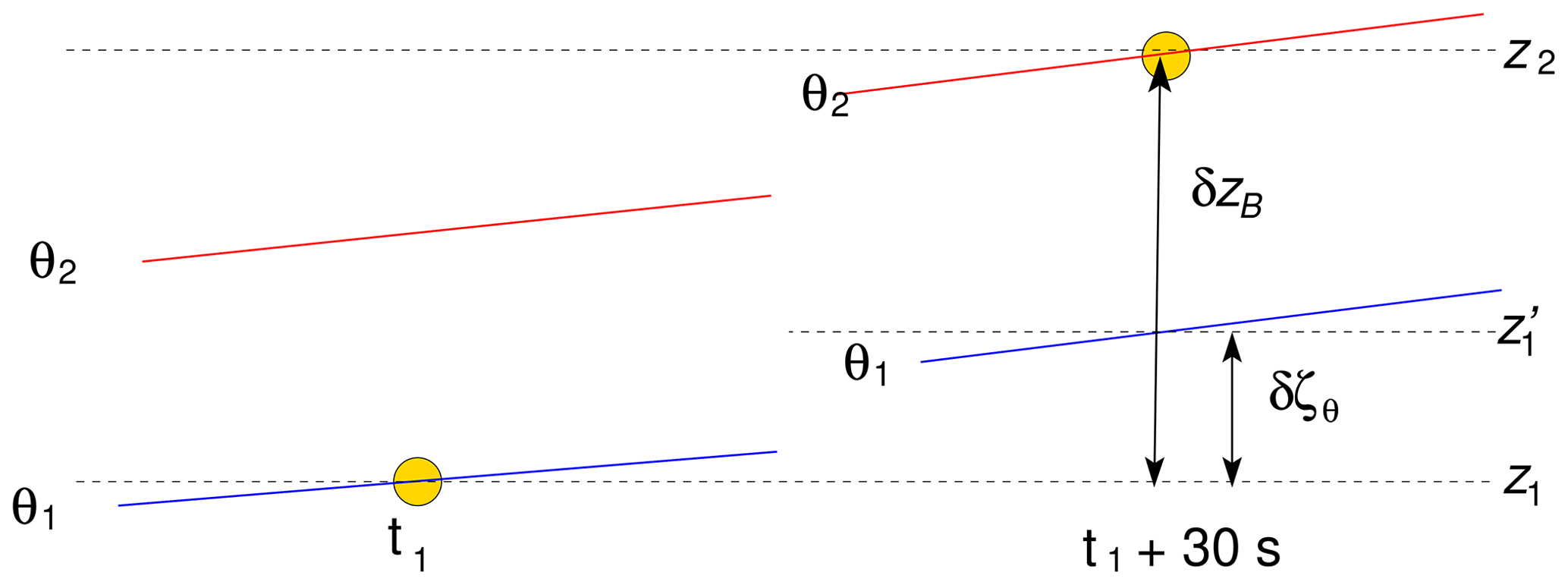
Figure 5 Schematic of the vertical displacement of an SPB. Between the measurement times t₁ and t₁+30 s, the vertical displacement of the SPB is δz_B, and the vertical displacement of the isentropic surface is δζ_θ.

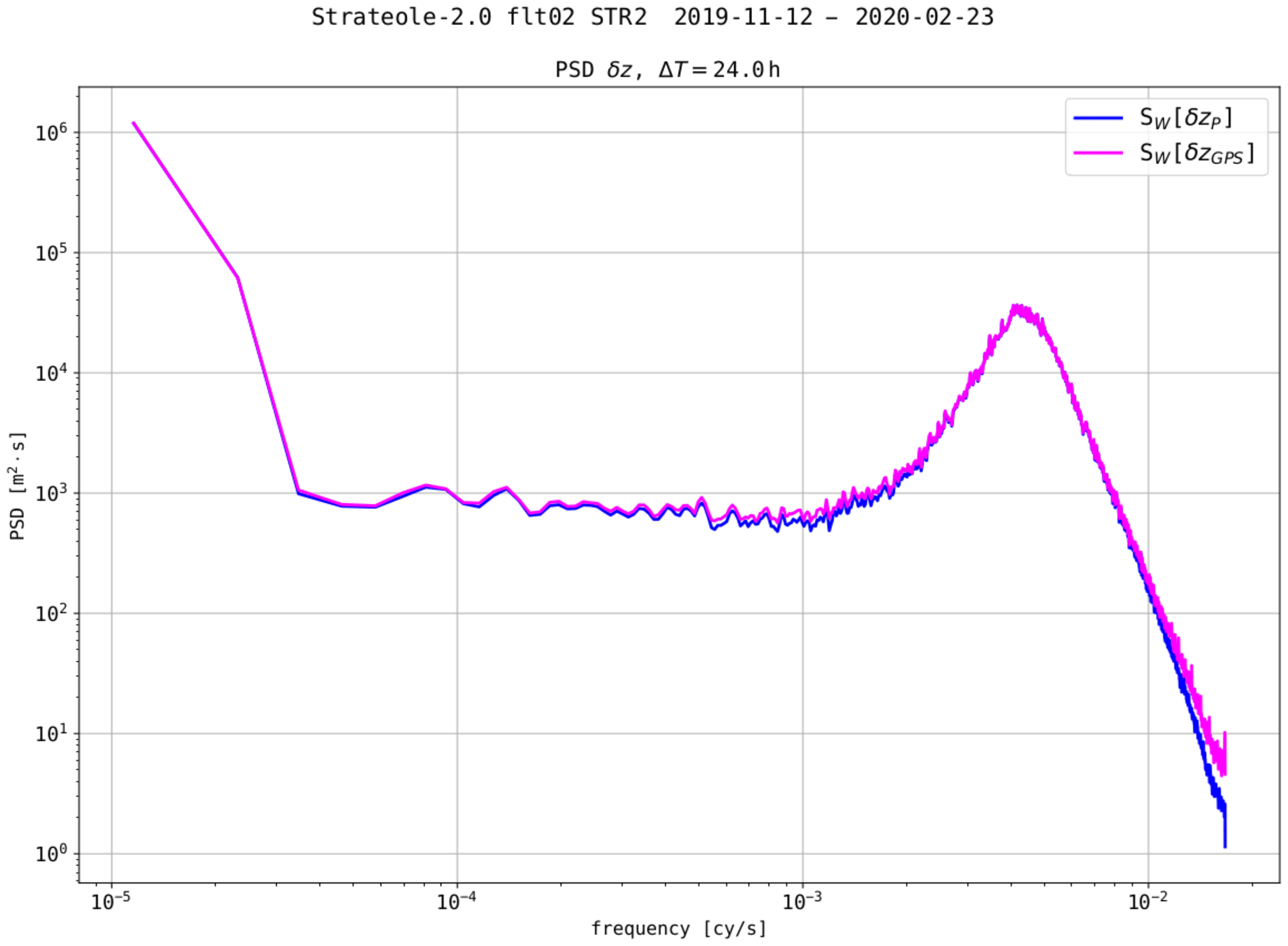
Figure 6 Power spectra of vertical increments of SPB heights, i.e., of vertical displacements between consecutive measurements (30 s), for flight 02_STR2.

3.2.2 The correlation method

The covariance of two quantities X and Y, is defined as follows:

$$\text{Cov}(X,Y)=E\left[\left(X-E\left[X\right]\right)\left(Y-E\left[Y\right]\right)\right].$$

Here, E is the mathematical expectation that is estimated by

$$\begin{array}{}\text{(5)}& \stackrel{\mathrm{̃}}{\text{Cov}}(X,Y)={\displaystyle \frac{\mathrm{1}}{N-\mathrm{1}}}\sum _{i=\mathrm{1}}^N(X-\stackrel{\mathrm{‾}}{X})(Y-\stackrel{\mathrm{‾}}{Y}),\end{array}$$

where N is the sample size. The Pearson correlation coefficient ${\mathit{\rho }}_P(X,Y)=\frac{\text{Cov}(X,Y)}{{\mathit{\sigma }}_X{\mathit{\sigma }}_Y}$ is estimated as follows:

$$\begin{array}{}\text{(6)}& r_P(X,Y)={\displaystyle \frac{\stackrel{\mathrm{̃}}{\text{Cov}}(X,Y)}{s_X{s}_Y}},\end{array}$$

where s_X is the estimate of the standard deviation σ_X of quantity X, i.e., $s_X=\sqrt{\stackrel{\mathrm{̃}}{\text{Cov}}(X,X)}$. A second correlation coefficient, the Spearman rank correlation coefficient, r_S(X,Y), has also been used in the present study. It is a measure of the statistical dependence between the rank of two variables X and Y. It is computed as the Pearson correlation between the rank values of those two variables:

$$\begin{array}{}\text{(7)}& r_S(X,Y)=r_P({\text{rk}}_X,{\text{rk}}_Y),\end{array}$$

where rk_X is the rank of variable X, i.e., sample X is replaced by the rank of X in the expression of r_P (Eq. 6). The use of the nonparametric Spearman correlation makes it possible to get rid of outliers in the time series (Spearman, 1904).

If the flow is stably stratified, the increments of potential temperature δθ are related to the vertical displacements of the SPB δz_B (Eq. 3). The covariance Cov(δθ,δz_B) reads as follows:

$$\begin{array}{}\text{(8)}& \begin{array}{rl}\text{Cov}\left(\mathit{\delta }\mathit{\theta },\mathit{\delta }{z}_{\mathrm{B}}\right)& =E\left[\mathit{\delta }\mathit{\theta }\times \mathit{\delta }{z}_{\mathrm{B}}\right]\\ & =E\left[\stackrel{\mathrm{‾}}{{\mathit{\theta }}_z}\left(\mathit{\delta }{z}_{\mathrm{B}}\times \mathit{\delta }{z}_{\mathrm{B}}-\mathit{\delta }{z}_{\mathrm{B}}\times \mathit{\delta }{\mathit{\zeta }}_{\mathit{\theta }}\right)\right].\end{array}\end{array}$$

Noting that (i) δζ_θ≪δz_B and (ii) the vertical oscillations of the balloon and the displacements of the isentropic surfaces are expected to be nonsynchronous because ω_B does not correspond to any atmospheric frequency (ω_B>N), we assume that the covariance E[δz_B×δζ_θ] is negligible compared with the variance of δz_B, i.e.,

$$\begin{array}{}\text{(9)}& \text{Cov}\left(\mathit{\delta }\mathit{\theta },\mathit{\delta }{z}_{\mathrm{B}}\right)=E\left[\stackrel{\mathrm{‾}}{{\mathit{\theta }}_z}\mathit{\delta }{z}_{\mathrm{B}}\times \mathit{\delta }{z}_{\mathrm{B}}\right].\end{array}$$

Notice that, under the above hypothesis, the covariance of a nonconservative measured quantity X (T, u, v) reads as follows:

$$\begin{array}{}\text{(10)}& \text{Cov}\left(\mathit{\delta }X,\mathit{\delta }{z}_{\mathrm{B}}\right)=E\left[\stackrel{\mathrm{‾}}{X_z}\mathit{\delta }{z}_{\mathrm{B}}\times \mathit{\delta }{z}_{\mathrm{B}}\right].\end{array}$$

If $\stackrel{\mathrm{‾}}{{\mathit{\theta }}_z}$ is positive in the time interval during which the covariance is estimated, Cov(δθ,δz_B) is expected to be positive. Moreover, if $\stackrel{\mathrm{‾}}{{\mathit{\theta }}_z}$ is strictly constant during the time interval,

$$\begin{array}{}\text{(11)}& \stackrel{\mathrm{‾}}{{\mathit{\theta }}_z}={\displaystyle \frac{\text{Cov}(\mathit{\delta }\mathit{\theta },\mathit{\delta }{z}_{\mathrm{B}})}{\text{Var}\left[\mathit{\delta }{z}_{\mathrm{B}}\right]}}.\end{array}$$

If $\stackrel{\mathrm{‾}}{{\mathit{\theta }}_z}$ is not strictly constant, as is very likely the case, the $\text{Cov}(\mathit{\delta }\mathit{\theta },\mathit{\delta }{z}_{\mathrm{B}})/\text{Var}\left[\mathit{\delta }{z}_{\mathrm{B}}\right]$ ratio can be interpreted as an estimate of the mean gradient $\langle \stackrel{\mathrm{‾}}{{\mathit{\theta }}_z}\rangle$ during the considered time interval at the flight level of the SPB. For a nonconservative quantities X,

$$\begin{array}{}\text{(12)}& \stackrel{\mathrm{‾}}{X_z}={\displaystyle \frac{\text{Cov}(\mathit{\delta }X,\mathit{\delta }{z}_{\mathrm{B}})}{\text{Var}\left[\mathit{\delta }{z}_{\mathrm{B}}\right]}}.\end{array}$$

In the ideal case where $\stackrel{\mathrm{‾}}{{\mathit{\theta }}_z}$ is constant and there is no instrumental noise, ${\mathit{\sigma }}_{\mathit{\delta }\mathit{\theta }}=\stackrel{\mathrm{‾}}{{\mathit{\theta }}_z}{\mathit{\sigma }}_{\mathit{\delta }{z}_{\mathrm{B}}}$ and the correlation coefficient $r_P(\mathit{\delta }\mathit{\theta },\mathit{\delta }{z}_{\mathrm{B}})=\mathrm{1}$, for all $\stackrel{\mathrm{‾}}{{\mathit{\theta }}_z}>\mathrm{0}$. This conclusion also holds for the Spearman correlation r_S if a linear relation is assumed between δθ and δz_B. If $\stackrel{\mathrm{‾}}{{\mathit{\theta }}_z}>\mathrm{0}$ but is no longer constant during the considered time interval, the correlation coefficient is smaller than 1 but is still positive, as the product δθ×δz_B is always positive. The correlation is further reduced, although remains positive, in the presence of uncorrelated noise (see Appendix B).

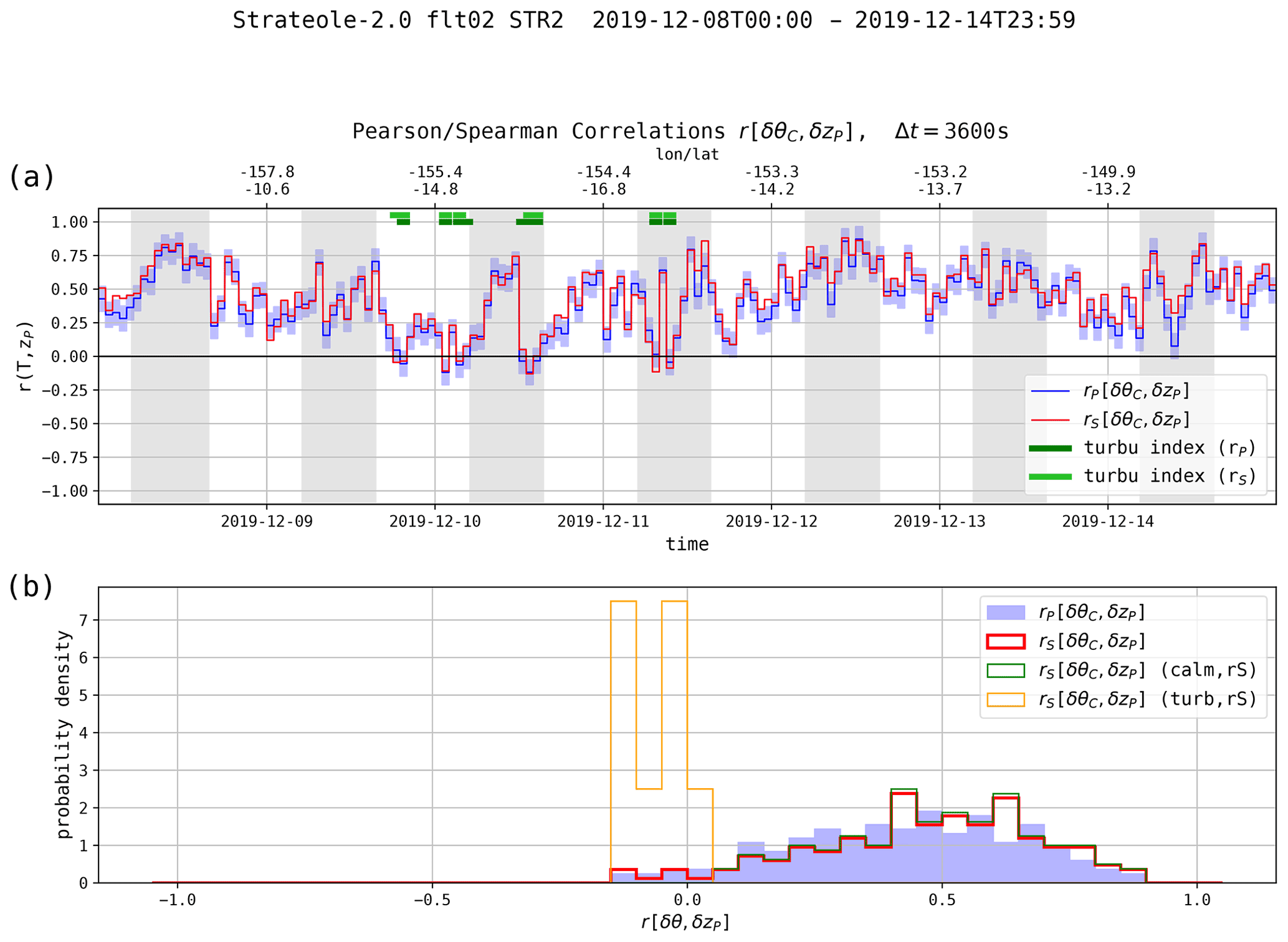
Figure 7 (a) Time series of correlation coefficients r_P and r_S applied to the increments' potential temperature derived from T_C and vertical displacements from z_P. The correlations are evaluated on 1 h time segments (120 samples). The time series runs for 7 d, from 8 to 15 December 2019. The gray vertical stripes indicate nighttime. The light blue shaded areas show the ±1 standard deviation interval for the Pearson correlations. (b) Histograms of the two correlation coefficients obtained during the week. The blue shading and thick red line correspond to all of the 1 h time segments, and the thin green and orange lines correspond to the calm (nonturbulent) and turbulent time intervals, respectively.

The first method to detect turbulent mixing is to check for a nonpositive correlation, i.e., a null or negative correlation, between δθ and δz_B. In order to infer if the null hypothesis H₀ has to be rejected – that is, if a positive correlation exists – a standard hypothesis test is performed. A confidence interval for the correlation coefficient is based on a Fisher transformation of the correlation estimate (Hotelling, 1953). Here, the H₀ hypothesis is rejected if the correlation estimate exceeds half of its standard deviation (unilateral test), with the corresponding confidence level being 69.15 %. If the H₀ hypothesis cannot be rejected, turbulent mixing is diagnosed, and the turbulence flag is set to “true”. Two turbulence indexes are built, either from the Pearson or Spearman correlations.

Figure 7 illustrates the time series (Fig. 7a) and histograms (Fig. 7b) of r_P and r_S during 1 week of flight 02_STR2. Both correlations are estimated over time segments of 1 h. The light blue shaded areas show the ±1 standard deviation interval for the Pearson correlations only. The thick green lines at the top of Fig. 7a display the time interval during which turbulence is detected, i.e., when the turbulence indexes are set to true.

As expected, the correlation coefficients are found to be positive most of the time. On a few occurrences during the time period shown in Fig. 7, turbulence is detected as the correlation coefficients approach zero. A good agreement in the time periods identified as turbulent is found regardless of the correlation method used.

3.2.3 The impact of instrumental noise on the correlation coefficients

The impact of measurement noise can be evaluated using the averages of the largest correlation coefficients, all corresponding to $\stackrel{\mathrm{‾}}{{\mathit{\theta }}_z}>\mathrm{0}$ a priori. The reader should recall that, without instrumental noise, the correlation (δθ,δz_B) is ideally 1 if $\stackrel{\mathrm{‾}}{{\mathit{\theta }}_z}>\mathrm{0}$ and remains constant over 1 h. As shown by Eq. (B1) in Appendix B, it is the ratio of the instrumental noise to the variance of the “geophysical” signal that appears in the correlation coefficient. In other words, the larger the amplitude of the balloon oscillations about their EDS, the less the measurement noise reduces the correlation coefficient.

The Spearman and Pearson correlation coefficients have been estimated for both potential temperature increments, δθ_C and δθ_S, and for both altitude increments, $\mathit{\delta }{z}_P=-\mathit{\delta }P/{\mathit{\rho }}_C$ and δz_GPS. Thus, four turbulence indexes coefficients are estimated. We have then averaged the 50 % of correlation coefficients with the largest values, i.e., the quantiles 50–100 of the coefficients, for each of the eight flights (Table 4). These averaged coefficients give information, at least relatively, on the quality of the data and on the performance of the turbulence estimators: the larger the correlations, the smaller the impact of instrumental noise.

Table 4 Averages of the 50 % of correlation coefficients with the largest values between δθ and δz. The Spearman and Pearson coefficients are displayed for the four combinations between δθ_S or δθ_C and δz_P or δz_GPS. About 1200 coefficients are averaged here for each flight. The largest correlation coefficient is displayed in bold for each flight. The larger the correlations, the smaller the impact of instrumental noise (see text).

Table 4 again illustrates that flight 03_TTL3 is abnormally noisy because of the poorer (potential) temperature measurements (see Table 2). Systematically, we observe the following:

1. the correlations are larger when using θ_C rather than θ_S,

2. there is a slight amelioration in using δz_P rather than δz_GPS,

3. the Spearman correlations (r_S) are slightly larger than the Pearson correlations (r_P).

We shall, therefore, prefer the Spearman estimator, using δT_C (and derived δθ_C) combined with δz_P, in evaluating both the correlations and the vertical gradients from which the turbulent indexes are estimated, as the impact of instrumental noise appears to be lower in this estimator.

3.2.4 The Richardson method

The second detection method is based on an evaluation of the local Richardson number (Ri). Notice that $\stackrel{\mathrm{‾}}{{\mathit{\theta }}_z}$ (Eq. 11) is the slope of a least squares linear regression between the 120 potential temperature increments (δθ) and vertical displacement increments (δz_B). This method of estimating the vertical gradient of the potential temperature is labeled the least squares fitting (LSF) method in the following. An alternative fitting method, the so-called Theil–Sen fitting (TSF) method, has also been used (Sen, 1968). The Theil–Sen estimator is defined as the median of the slopes of all lines through pair of points of the sample. It is a nonparametric and robust method that is almost insensitive to outliers. Both fitting methods have been applied to estimate the vertical gradients of several measured quantities, such as T and P or the horizontal wind velocities u and v (Eq. 12).

Two estimates of the mean Brunt–Väisälä frequency are thus computed with either the LSF or the TSF, applied to δT_C and δz_P, which were identified as the less noisy estimates of the air temperature and vertical displacements, respectively (see Tables 2 and 3). The squared shear, evaluated from the vertical gradients of the horizontal velocities, is obtained similarly. Hence, two turbulence indexes are built using LSF and TSF estimates of the Richardson number and are set to true if $\mathit{Ri}\le \mathrm{1}/\mathrm{4}$.

Figure 8a displays the vertical gradients of temperature for the same 1-week time series as that shown in Fig. 7. Estimates are shown for only the thermocouple temperatures and vertical displacements obtained with the pressure increments. Time series (not shown) obtained from other pairs of variables (using T_S or T_C or using z_GPS or z_P) are very similar to the one presented, regardless of the fitting method used. The uncertainty (±1 standard deviation) is shown in light red for the LSF estimator. The turbulence detection criteria based on the Richardson number are also displayed (thick green lines at the top of the figure). Figure 8b shows the probability distribution functions (PDFs) of the vertical gradients of temperature shown above (blue shading and thick curve). PDFs corresponding to turbulent and calm (i.e., nonturbulent) periods according to the Richardson number criterion are also displayed using thin lines.

First, it should be noticed that the choice of the LSF or TSF estimates for the vertical gradient of temperature or for the turbulence index has only a minor impact. Similarly, the choice of parameters (z_P or z_GPS, T_C or T_S) and any combination of those has little influence on the detection of turbulence layers (not shown). Figure 8 also clearly illustrates that the time periods flagged as turbulent by the Richardson number index are associated with the small-value tail of the temperature gradient PDF ($\mathrm{d}T/\mathrm{d}z\lesssim -\mathrm{10}$ K km⁻¹). Finally, those time periods are essentially the same as the one shown in Fig. 7, obtained using the correlation method.

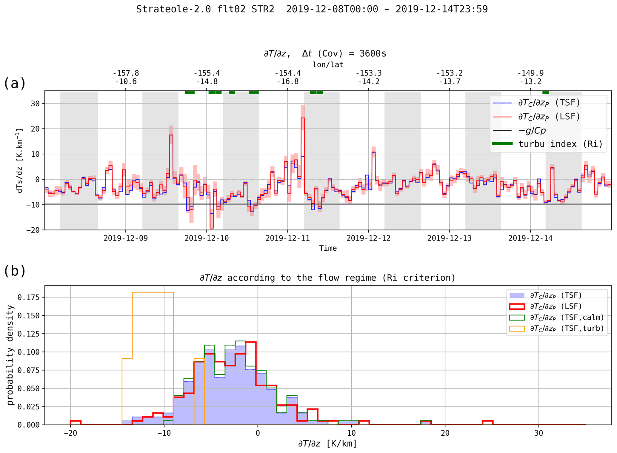
Figure 8 (a) Time series of $\partial T/\partial z$ estimated by two respective fitting methods, least squares fitting (LSF) and Theil–Sen fitting (TSF), from T_C and z_P. Linear fits are performed on 1 h time segments (120 samples). The light red shaded areas show the ±1 standard deviation interval for the LSF estimates. (b) Histograms of the temperature gradients from the two respective methods. The histograms corresponding to the turbulent and laminar time segments are also plotted (light curves).

4 Results

4.1 Turbulence detection with the correlation method

Figure 9a displays the time series of both the Spearman and Pearson correlation coefficients between δθ_C and δz_P for the whole flight 02_STR2. As done previously, the correlations are estimated on time segments of 1 h (120 samples). They range from $\sim -\mathrm{0.5}$ to 0.96. Both time series exhibit very similar variations, showing time intervals lasting several days with relatively large correlations (>0.7) and short bursts of time with low or even negative correlations. Two turbulence indexes inferred from the Spearman and Pearson correlation methods are shown as thick green lines at the top of Fig. 9a. The fraction of time during which the flow is detected as turbulent for flight 02_STR2 is 4.5 % (4.4 %) from the Spearman (Pearson) correlations (see Table 5). Time series and histograms of correlations obtained using measurements of δθ_S or δz_GPS (not shown) provide time series that are almost indistinguishable from those shown in Fig. 9.

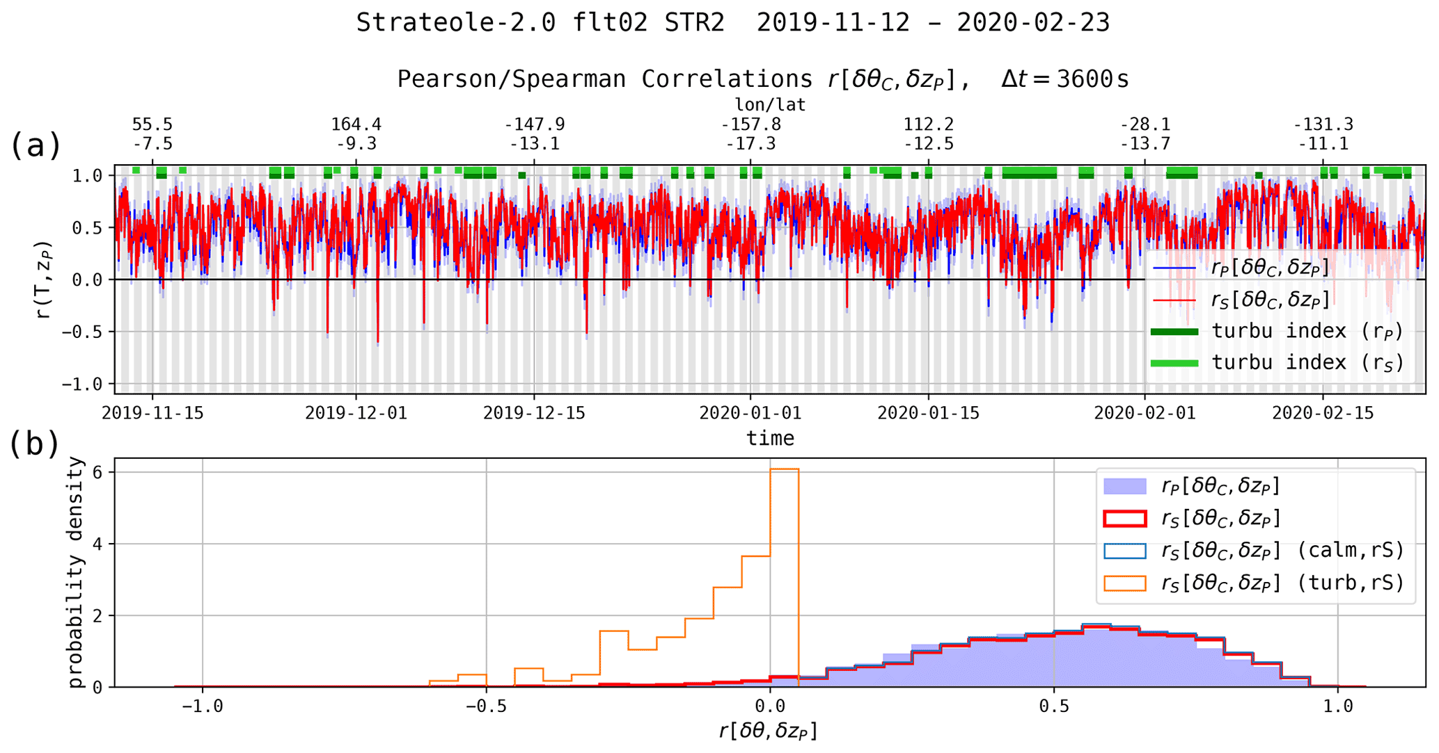
Figure 9 (a) Time series of the Spearman and Pearson correlation coefficients between δθ_C and δz_P during flight 02_STR2 (103 d). The turbulence indexes deduced from the two correlations are shown (thick green lines at the top of the plot). (b) Histograms of the Spearman (thick line) and Pearson (filled) coefficients for flight 02_STR2. Also shown are the histograms corresponding to the turbulent and laminar cases (thin lines). The time series and histograms of the two correlation coefficients are very similar, even though a few differences in turbulence detection are visible.

Figure 9b shows the PDFs of the two correlation coefficients over the whole flight (blue shading and thick red line). Both distributions are observed to be almost identical, although r_S is slightly and systematically larger than r_P for correlations larger than 0.5. The average values for both correlation coefficients are close: $\stackrel{\mathrm{‾}}{r_S[\mathit{\delta }{\mathit{\theta }}_C,\mathit{\delta }{z}_P]}=\mathrm{0.50}$ and $\stackrel{\mathrm{‾}}{r_P[\mathit{\delta }{\mathit{\theta }}_C,\mathit{\delta }{z}_P]}=\mathrm{0.48}$. The thin lines show the PDFs of r_S for solely turbulent (orange) and solely laminar time periods (green). The PDFs associated with the laminar time periods are almost identical to those of the whole flight, as they correspond to about 95 % of the data. The turbulent time periods correspond only to the small-value tail of the overall distribution.

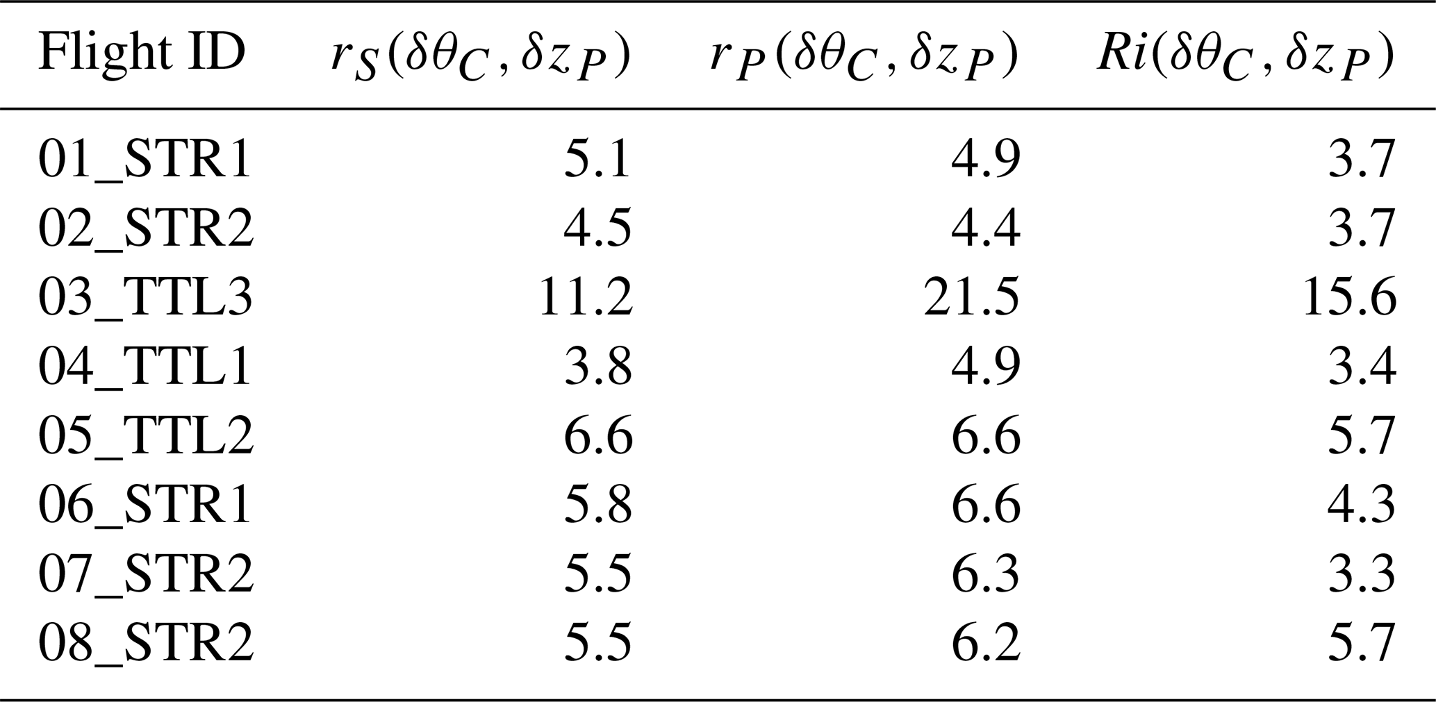
The fractions of time during which the flow is found to be turbulent using the correlation method are reported in Table 5 for the eight flights of the campaign. Overall, they look very consistent, typically ranging between 4.5 % and 6.5 %, with the exception of flight 03_TTL3, which is associated with noisier temperature measurements.

Table 5 Fraction of time (percent) during which the flow is found to be turbulent. Turbulence is diagnosed from the correlation method based of δθ_C and δz_P (second and third columns) and from the Ri(δT_C,δz_P) criterion (last column).

4.2 Estimations of the vertical temperature gradient with the fitting methods

Figure 10 shows estimates of $\partial T/\partial z$ for flight 02_STR2 inferred from linear fitting of the increments of temperature and vertical displacements during hourly intervals. More precisely, Fig. 10a shows the vertical temperature gradient obtained with the TSF method applied to δT_C and δz_P. Time series obtained using other combinations of measured variables and fitting methods (not shown) are almost indistinguishable from the one shown in Fig. 10. The dry adiabatic lapse rate $\mathrm{\Gamma }=-g/c_P$ is also indicated as a black line. The turbulence index based on Ri is shown as a thick green discontinuous line at the top of Fig. 10a. Figure 10b shows the PDFs of $\partial T/\partial z$ for the whole flight and for the respective calm and turbulent time periods. The distribution of $\partial T/\partial z$ is found to be very asymmetric, with the mode being close to −4 K km⁻¹. Most of the turbulent cases are associated with $\partial T/\partial z<\mathrm{\Gamma }$, with a few of them being associated with $\partial T/\partial z>\mathrm{\Gamma }$. The cumulative distribution functions (CDFs) of the temperature gradients are displayed in Fig. 10c. About 80 % of the detected turbulent cases, associated with Ri<0.25, correspond to a super-adiabatic temperature gradient.

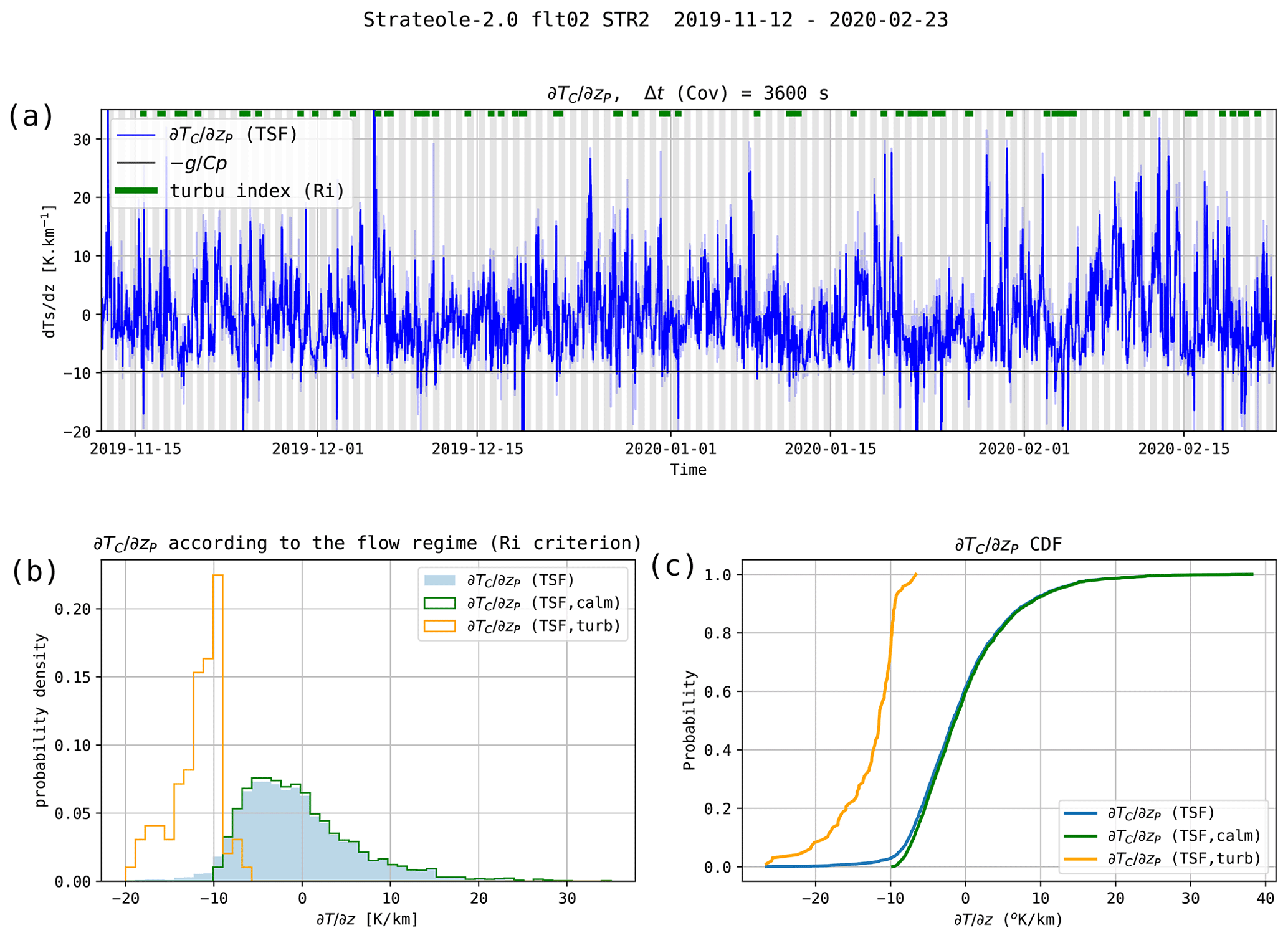
Figure 10 (a) Two estimates of $\partial T_C/\partial z_P$ for flight 02_STR2, from the linear fitting of T_C and δz_P at hourly intervals. The black line shows the adiabatic lapse rate $-g/c_P$. The Ri turbulence index is drawn on the top of the figure as a thick green discontinuous line. (b) Histograms of $\partial T_C/\partial z_P$ for all of the time intervals (blue shading) and for the respective laminar and turbulent cases (thin lines). (c) CDFs of the temperature gradients.

Based on $\partial T/\partial z$ estimates, the Brunt–Väisälä and NBO frequencies can be evaluated, see Eqs. (1) and (2). Figure 11 displays the squared Brunt–Väisälä (N²), the theoretical NBO (${\mathit{\omega }}_{\mathrm{NBO}}^{\mathrm{2}}$), and the observed balloon (${\mathit{\omega }}_{\mathrm{B}}^{\mathrm{2}}$) frequencies for the whole 02_STR2 flight. The Brunt–Väisälä and NBO frequencies are deduced from the hourly estimates of $\partial T/\partial z$. The observed balloon frequencies are directly estimated from observations of the balloon oscillations (Fig. 3). A 60 min running average is then applied to the raw ω_B time series. The three frequencies are close to but distinct from one another, with the observed balloon frequency ranging between N and ω_NBO. The CDF of frequency ratios (Fig. 11c) reveals that ∼95 % of the measured ω_B are smaller than the ω_NBO estimates and that 19 % of ω_B are smaller than N. This property is consistent with numerical simulations of the motion of a spherical SPB assuming that atmospheric forcing occurs at frequencies lower than the Brunt–Väisälä frequency (Podglajen et al., 2016, in particular see their Supplement).

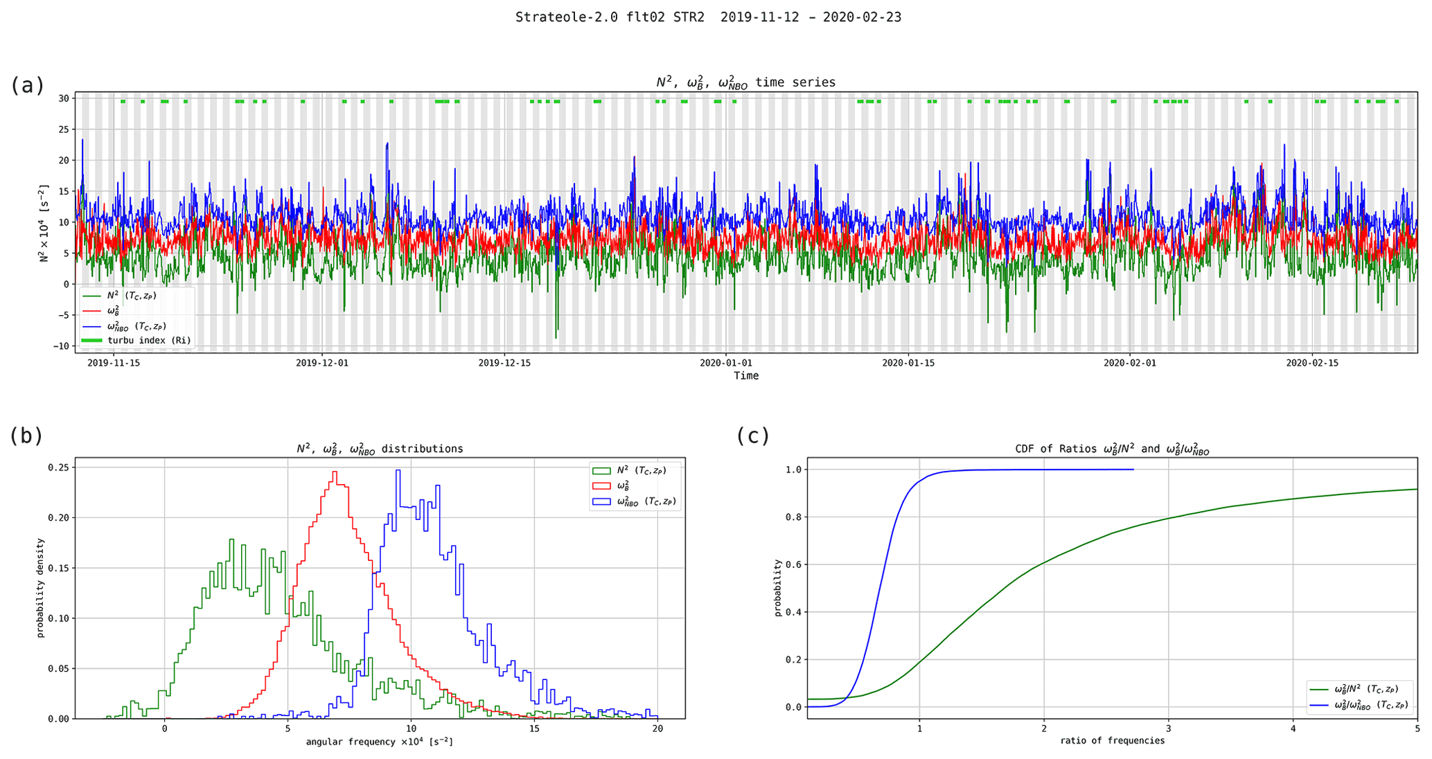
Figure 11 Times series (a) and histograms (b) of the Brunt–Väisälä, NBO, and observed balloon frequencies. The Brunt–Väisälä and NBO frequencies are deduced from the estimates of $\partial T/\partial z$ from Cov(δT_C,δz_P). (c) CDF of the ${\mathit{\omega }}_{\mathrm{B}}^{\mathrm{2}}/N^{\mathrm{2}}$ and ${\mathit{\omega }}_{\mathrm{B}}^{\mathrm{2}}/{\mathit{\omega }}_{\mathrm{NBO}}^{\mathrm{2}}$ ratios.

Figure 12 shows the histograms of $T_z=\partial T_C/\partial z_P$ for flight 3 obtained from the TSEN measurements (TSF method) and from the RACHuTS temperature profiles – down to 2 km below the balloon. The vertical gradients of the RACHuTS temperature are estimated using 30 m vertical segments. The RACHuTS histogram has common features with the TSEN histograms: an asymmetric distribution, the same negative modes, and a sharp transition around −10 ^∘C km⁻¹. These distributions are considered to be consistent, despite the fact that they are not obtained in the same altitude domain nor simultaneously.

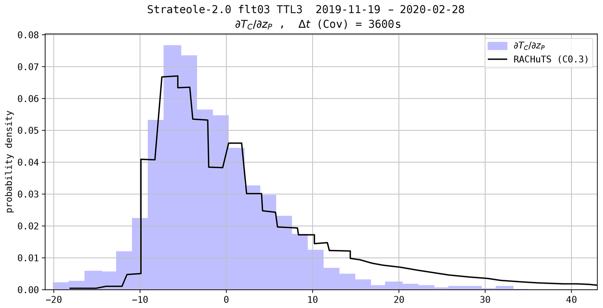
Figure 12 Histograms of $\partial T/\partial z_P$ from the covariance of the TSEN measurements (blue shading) and from the RACHuTS temperature profile (black line). The two histograms have common characteristics, despite the fact that they are not obtained at the same altitude levels.

4.3 Turbulence detection with the Ri method

Figure 13 shows estimates of the Richardson number along flight 02_STR2, obtained using either the LSF or TSF estimates, with T_C, z_P, u, and v observations. The corresponding two turbulence indexes ($\mathit{Ri}⩽\mathrm{1}/\mathrm{4}$) are also shown in Fig. 13a (green thick line). Figure 13b displays the histograms of the two Ri estimates. The time series and histograms of the two Ri estimates look very similar, even though a few differences in the turbulence detection are visible.

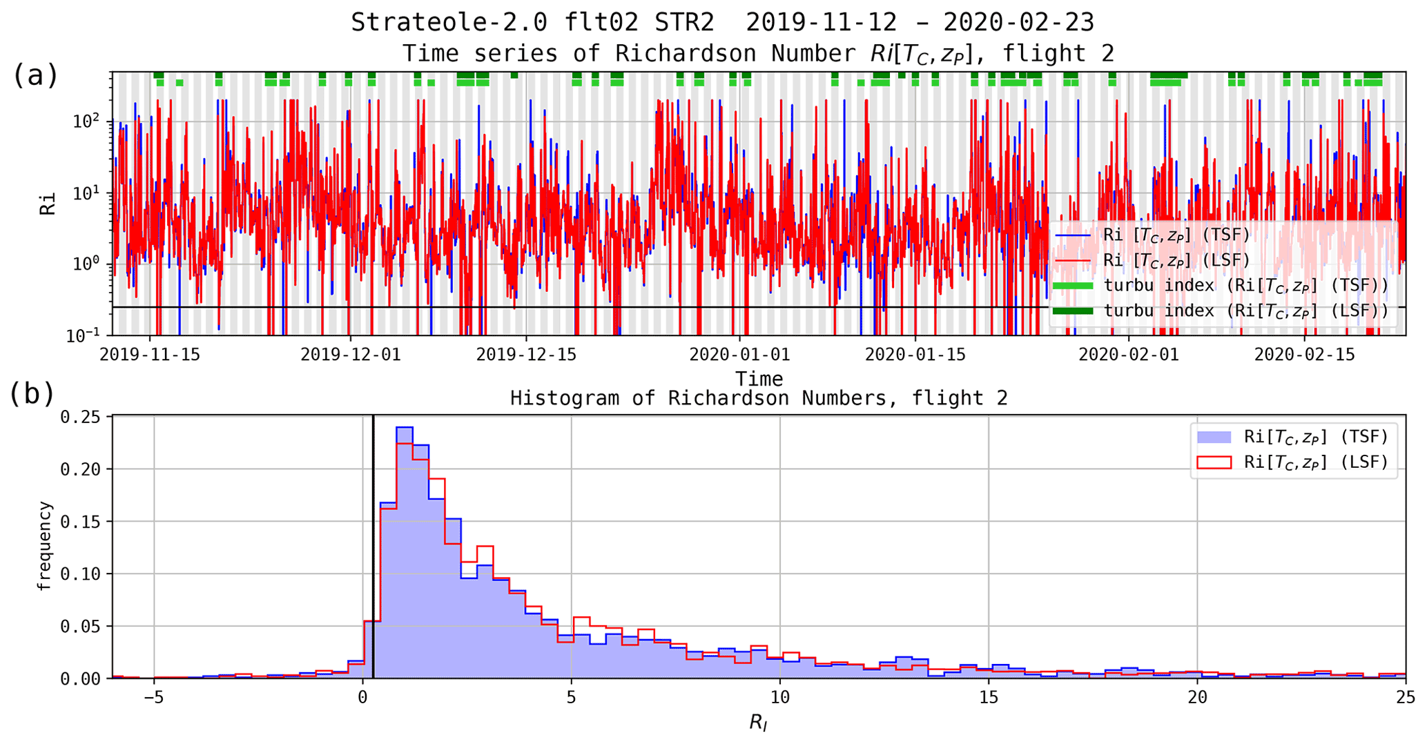
Figure 13 (a) Richardson number estimates from T_C, u, v, and z_P using the respective least squares fitting (LSF) and Theil–Sen fitting (TSF) methods. The thick black line shows the threshold Ri=0.25. The two inferred turbulence indexes are shown (thick green lines at the top of the plot). (b) Histograms of the two Richardson number estimates.

As shown in Table 5, the fraction of time during which the flow is found to be turbulent according to the Ri criterion is 3.7 % for flight 02_STR2. More generally, the detection of turbulent flow during the Strateole-2 C0 campaign ranges from 3.3 % to 5.7 % of the time, with the exception of flight 03_TTL3.

5 Discussion

5.1 Possible impact of wake on the temperature measurements

Due to the vertical oscillations of the balloon, the T sensors were possibly in the wake of the balloon or of the flight chain. Note that we expect the balloon wake to be warm during daytime and cold during nighttime, with the balloons being cooler than the ambient air during nighttime.

The temperature sensors were located 27 m below the balloon base (except for during the 03_TTL3 flight) and 15 m below the EUROS gondola. The diameter of the balloons was either 11 m (TTL) or 13 m (STR). On all but the TTL3 flights, the T sensors were located 7 m below the last gondola in the flight chain. Flight 03_TTL3, carrying the RACHuTS system, is an exception, as the temperature sensors were located 30 cm from the EUROS gondola.

The question of the possible impact of the wake on temperature measurements has been taken into account. Indeed, we have calculated the statistics, vertical gradients, and correlations, considering only the downward phases of the oscillations, i.e., when the temperature sensors (which are located at the lower end of the flight chain) sample “fresh” air if a minimum shear exists. The resulting time series (not shown) are noisier because we only consider about half of the samples. However, both time series of correlations and temperature gradients have similar characteristics to those calculated when considering all samples, showing the same succession of stable and unstable periods. Therefore, we conclude that the impact of the wake does not significantly affect the estimated statistics, correlations, nor covariances, and, due to the increase in noise, we choose to consider all of the samples.

5.2 Comparison of the turbulence indexes

Table 6 shows the percentage of identical detections (laminar or turbulent) of the four turbulence indexes (r_P, r_S, Ri_LSF, and Ri_TSF) for the eight balloon flights. The percentage of similar detections ranges from 97.9 % (r_S vs. Ri_LSF) to 99.07 %. However, as pointed out by an anonymous reviewer, such overall agreement does not imply equally good agreement between estimators when turbulence is detected. Choosing Ri_TSF as a reference, we compared the diagnoses with the other three estimators (Ri_LSF, r_P, and r_S). Figure 14 shows the percentages of similar and different detections when the flow is diagnosed as turbulent (T) or laminar (L). It reveals that the detections are similar for more than 99 % of cases if the flow is diagnosed as laminar. If the flow is diagnosed as turbulent, the rate of identical detections drops to about 80 %, with the comparison being the worst for r_P (76 %) and comparable for r_S and Ri_LSF (83.2 % and 85.4 %, respectively). We believe that these differences mainly result from the fact that the threshold values, zero correlation or Ri=0.25, correspond to the tails of the distributions of these estimates (see the histograms in Figs. 9 and 13). When the atmosphere is weakly stratified, threshold effects are likely to be important, leading to some differences in the diagnoses of flow conditions.

We also found that the time fraction of turbulent episodes obtained by the Ri criterion is almost always smaller than that obtained by the correlation methods (Table 5). This can be partly due to the threshold values of the hypothesis tests of a null correlation (i.e., to the choice of a confidence interval).

Table 6 Percentage of identical turbulence detections from four turbulence index using (T_C, z_P) for flight 02_STR2.

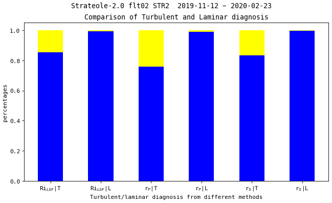
Figure 14 Percentages of true (similar) and false (different) detections for turbulent (T) and laminar (L) episodes diagnosed by the Ri_TSF criterion. The three estimators, Ri_LSF, r_P, and r_S, are compared to Ri_TSF. The rate of agreement is larger than 99 % in the case of laminar flow and about 80 % in the case of turbulent flow.

5.3 Occurrences of negative values for Ri and N²

The time series of N² (Fig. 11) and Ri (Fig. 13) show some negative values. For the considered flight (02_STR2), the occurrence frequency of negative N² is 3.4 % (from the Theil–Sen regression performed on T_C and z_P). Such a negative Ri (N²) can result from both the dispersion of the temperature gradient estimates and the occurrence of episodes of unstable stratification.

Negative estimates of N² (or Ri) could be due to the precision of the temperature gradient estimates, which are expected to be scattered around a value close to −10 ^∘C km⁻¹ in the case of neutral stratification. Temperature gradients are estimated from the covariance of temperature increments and displacements, with these covariances scattered around their mean values. As a result, N² estimates can be negative even if the stratification is neutral or nearly neutral.

However, unstable stratifications (N²<0) seem to occur in the lower stratosphere, as they have been reported in the literature. For instance, the detection of turbulence by the Thorpe method from in situ measurements is based on observations of $\partial \mathit{\theta }/\partial z<\mathrm{0}$, i.e., N²<0 (Thorpe, 1977). The probability of occurrence of such unstable layers likely depends on the vertical resolution of the profiles (e.g., Wilson et al., 2011) but is not zero. In the lower stratosphere, KHIs are expected to be the main source of instability. For KHIs, turbulence is expected to be triggered for $\mathrm{0}<\mathit{Ri}<\mathrm{1}/\mathrm{4}$, i.e., for N²>0; however, once it is developed, the stratification can become almost neutral (N²≈0) or even unstable (N²<0) as a result of stirring and mixing. Therefore, it is plausible that the occurrence of unstable episodes may also contribute to negative values of N² or Ri estimated from covariances.

Numerical simulations indicate that large temperature gradients are expected at the edges of turbulent layers (Fritts et al., 2003; Werne and Fritts, 1999). These strong temperature gradients are also commonly observed from radiosonde profiles when turbulence detection is performed by the Thorpe method (e.g., Luce et al., 2002). It is clear that sampling by balloons drifting within an air mass, and not cutting vertically through it as done by a radiosonde, will not allow one to identify turbulence from these sharp temperature gradients at the layer edges. Only the central part of the turbulent region, in which stratification is almost zero, can be identified as turbulent.

5.4 Spatial inhomogeneity of turbulence detections

The detection of turbulent episodes is far from uniform around the globe. Figure 15 shows the positions of turbulence detections (green dots) for the eight flights of the C0 campaign. Turbulence detections seem to be very rare over some regions (e.g., the southern Atlantic Ocean) and quite frequent over other regions (e.g., the Maritime Continent or the western Pacific). At the present stage, this result is only qualitative; however, interestingly, these inhomogeneities are likely related to the causes of the turbulence occurrences (see for instance Fritts and Alexander, 2003). A study examining processes that cause turbulence in the UTLS is in progress.

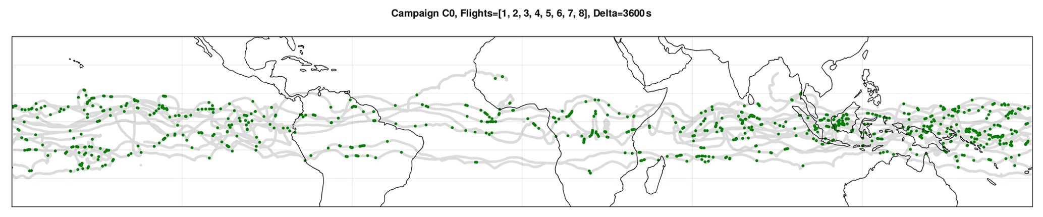
Figure 15 The positions of turbulent patches are shown as green dots for the eight flights of the C0 campaign. Each dot corresponds to a 1 h time interval. The detections are based on the Ri_TSF criterion. The detected turbulence episodes are far from uniform around the globe.

6 Summary and concluding remarks

The present paper dealt with the detection of turbulence on superpressure balloon flights that drift for several months in the UTLS. During the Strateole-2 C0 campaign, eight SPBs were launched. Statistical methods to infer the flow regime, either laminar or turbulent, in which the SPBs were drifting are described. Some properties of the local stratification of the flow are also inferred. These methods are based on in situ GPS altitude, pressure, and temperature measurements, which were performed on all of the SPBs of the Strateole-2 C0 campaign with a time resolution of 30 s.

We make use of the SPB oscillations about their equilibrium density surface, which typically enable SPBs to vertically explore the atmosphere over 30 m (peak-to-peak displacements). The observed periods of oscillation, ∼220 s on average, are significantly smaller than the Brunt–Väisälä period. The large amplitude of these balloon motions at frequencies higher than the Brunt–Väisälä frequency (where turbulence is expected to occur) makes it very difficult, if not impossible, to detect turbulence from the direct characterization (i.e., from the variance or power spectra) of high-frequency fluctuations. On an other hand, thanks to the vertical motions of the SPBs around their EDS, the vertical gradients of any measured quantity can be estimated, either via the covariance between the increments of this quantity and those of the vertical displacements or, equivalently, via the linear fit between these two increments. For the present study, covariances and linear fits have been estimated on data segments of 1 h, i.e., 120 data samples.

Several turbulence indexes (true or false) are defined and compared. A first index is based on an inference test on the correlation between potential temperature and altitude increments. A null correlation is expected in the case of turbulent mixing, as the vertical gradient of potential temperature tends to zero. Two correlation coefficients, the Pearson and Spearman coefficients, have been tested and compared for the eight balloon flights. Alternatively, based on a linear fit between increments, vertical temperature gradients and horizontal wind can be evaluated at 1 h intervals, from which the local Richardson number can be deduced. A second turbulence index is then based on the criterion Ri<0.25. These different turbulence indexes compare well, as they coincide for more than 97 % of cases.

SPBs sample the atmosphere without any spatial or temporal sampling bias, drifting nights and days, over oceans and continents, and above convective and non-convective regions. The fraction of time during which the flow is found to be turbulent in the lower stratosphere appears to be quite small, ranging from 3.3 % to 6.6 %. Because of the lack of sampling bias, such a fraction of time can be interpreted as a fraction of space. The probability of occurrence of instabilities is far from being uniform in time (or space). Periods of several days are frequently observed during which the atmosphere is stable, i.e., without any instability. On the other hand, during certain periods, the frequency of instabilities appears to be quite high. At first sight, these differences could be attributable to the underlying deep convection, as observed, for example, when the balloons are flying over the Maritime Continent. However, this remains a very preliminary conclusion that needs to be substantiated in future work.

Appendix A: Estimation of the uncorrelated noise

The measured signal is assumed to contain an uncorrelated and centered noise contribution. This noise level is estimated on short data segments (∼20 data samples), with the useful signal being described by a polynomial fit of degree n. The time series of quantity X reads

$$\begin{array}{}\text{(A1)}& \underset{\mathrm{¯}}{X_i}=X_i+{\mathit{\xi }}_i\left(\mathrm{1}\le i\le n\right),\end{array}$$

where $\underset{\mathrm{¯}}{X_i}$ is the measured signal, and ξ_i is an uncorrelated noise of variance σ_ξ. The measured first increment reads

$$\begin{array}{}\text{(A2)}& \mathit{\delta }\underset{\mathrm{¯}}{X_i}=X_{i+\mathrm{1}}-X_i+{\mathit{\xi }}_{i+\mathrm{1}}-{\mathit{\xi }}_i.\end{array}$$

If X_i is constant, i.e., $X_{i+\mathrm{1}}-X_i=\mathrm{0}$, the variance of $\mathit{\delta }\underset{\mathrm{¯}}{X_i}$ reduces to

$$\begin{array}{}\text{(A3)}& \text{Var}\left[\mathit{\delta }\underset{\mathrm{¯}}{X_i}\right]=\mathrm{2}\text{Var}\left[\mathit{\xi }\right]=\mathrm{2}{\mathit{\sigma }}_{\mathit{\xi }}^{\mathrm{2}}.\end{array}$$

The measured second increment reads

$$\begin{array}{}\text{(A4)}& \begin{array}{rl}{\mathit{\delta }}^{\mathrm{2}}\underset{\mathrm{¯}}{X_i}& =\mathit{\delta }\underset{\mathrm{¯}}{X_{i+\mathrm{1}}}-\mathit{\delta }\underset{\mathrm{¯}}{X_i}\\ & =X_{i+\mathrm{2}}-\mathrm{2}{X}_{i+\mathrm{1}}+X_i+{\mathit{\xi }}_{i+\mathrm{2}}-\mathrm{2}{\mathit{\xi }}_{i+\mathrm{1}}+{\mathit{\xi }}_i.\end{array}\end{array}$$

If X_i varies according a linear trend, i.e., $X_{i+\mathrm{2}}-\mathrm{2}{X}_{i+\mathrm{1}}+X_i=\mathrm{0}$, the variance of ${\mathit{\delta }}^{\mathrm{2}}\underset{\mathrm{¯}}{X_i}$ reduces to

$$\begin{array}{}\text{(A5)}& \begin{array}{rl}\text{Var}\left[{\mathit{\delta }}^{\mathrm{2}}\underset{\mathrm{¯}}{X_i}\right]& =\text{Var}\left[\mathit{\xi }\right]+\mathrm{4}\text{Var}\left[\mathit{\xi }\right]+\text{Var}\left[\mathit{\xi }\right]\\ & =\sum _{k=\mathrm{0}}^{\mathrm{2}}{\left(\begin{array}{c}\mathrm{2}\\ k\end{array}\right)}^{\mathrm{2}}{\mathit{\sigma }}_{\mathit{\xi }}^{\mathrm{2}}=\mathrm{6}{\mathit{\sigma }}_{\mathit{\xi }}^{\mathrm{2}}.\end{array}\end{array}$$

The measured nth increment reads

$$\begin{array}{}\text{(A6)}& \begin{array}{rl}{\mathit{\delta }}^n\underset{\mathrm{¯}}{X_i}& ={\mathit{\delta }}^{n-\mathrm{1}}\underset{\mathrm{¯}}{X_{i+\mathrm{1}}}-{\mathit{\delta }}^{n-\mathrm{1}}\underset{\mathrm{¯}}{X_i}=\sum _{k=\mathrm{0}}^n(-\mathrm{1}{)}^{n-k}\left(\begin{array}{c}n\\ k\end{array}\right)X_{i+k}\\ & +\sum _{k=\mathrm{0}}^n(-\mathrm{1}{)}^{n-k}\left(\begin{array}{c}n\\ k\end{array}\right){\mathit{\xi }}_{i+k}.\end{array}\end{array}$$

If X_i is described by a polynomial of degree n−1, the first term on the right-hand side of Eq. (A6) cancels, and the variance of ${\mathit{\delta }}^n\underset{\mathrm{¯}}{X_i}$ reduces to

$$\begin{array}{}\text{(A7)}& \text{Var}\left[{\mathit{\delta }}^n\underset{\mathrm{¯}}{X_i}\right]=\sum _{k=\mathrm{0}}^n{\left(\begin{array}{c}n\\ k\end{array}\right)}^{\mathrm{2}}{\mathit{\sigma }}_{\mathit{\xi }}^{\mathrm{2}}.\end{array}$$

Increasing the order of differentiation enhances the relative contribution of the uncorrelated signal in the time series. After several differentiations, the variance of the differentiated time series is expected to converge to the weighted variance of the uncorrelated noise.

Appendix B: Impact of instrumental noise on the correlation coefficients

The Pearson or Spearman correlation coefficients (ρ_P and ρ_S, respectively) will be reduced because of uncorrelated noise in the time series of δz_B and δθ. A simplistic model may help to illustrate this assertion. Let us note $\underset{\mathrm{¯}}{\mathit{\theta }}$, the measured potential temperature, and $\underset{\mathrm{¯}}{z_{\mathrm{B}}}$, the measured altitude of the balloon. Assume that $\underset{\mathrm{¯}}{\mathit{\theta }}$ can be analyzed as $\underset{\mathrm{¯}}{\mathit{\theta }}=\mathit{\theta }+\mathit{\eta }$, where θ is the real value and η is a centered random noise. Similarly, $\underset{\mathrm{¯}}{z_{\mathrm{B}}}=z_{\mathrm{B}}+\mathit{\zeta }$. The variance of the measured increments $\mathit{\delta }\underset{\mathrm{¯}}{X}$ (X=θ or z_B) reads

$$\text{Var}\left[\mathit{\delta }\underset{\mathrm{¯}}{X}\right]=\text{Var}\left[\mathit{\delta }X\right]+\mathrm{2}{\mathit{\sigma }}_X^{\mathrm{2}},$$

where σ_X is the standard deviation of the random noise on X. Also, $\text{Cov}[\mathit{\delta }\underset{\mathrm{¯}}{\mathit{\theta }},\mathit{\delta }\underset{\mathrm{¯}}{z_{\mathrm{B}}}]=\text{Cov}[\mathit{\delta }\mathit{\theta },\mathit{\delta }{z}_{\mathrm{B}}]$. The expectation of the Pearson correlation coefficient ${\mathit{\rho }}_P[\underset{\mathrm{¯}}{\mathit{\delta }\mathit{\theta }},\underset{\mathrm{¯}}{\mathit{\delta }{z}_{\mathrm{B}}}]=\text{Cov}[\mathit{\delta }\underset{\mathrm{¯}}{\mathit{\theta }},\mathit{\delta }\underset{\mathrm{¯}}{z_{\mathrm{B}}}]/\left(\text{Var}\right[\mathit{\delta }\underset{\mathrm{¯}}{\mathit{\theta }}\left]\text{Var}\right[\mathit{\delta }\underset{\mathrm{¯}}{z_{\mathrm{B}}}]{)}^{\mathrm{1}/\mathrm{2}}$ reads

$$\begin{array}{}\text{(B1)}& \begin{array}{rl}& {\mathit{\rho }}_P[\underset{\mathrm{¯}}{\mathit{\delta }\mathit{\theta }},\underset{\mathrm{¯}}{\mathit{\delta }{z}_{\mathrm{B}}}]\\ & ={\displaystyle \frac{{\mathit{\rho }}_P[\mathit{\delta }\mathit{\theta },\mathit{\delta }{z}_{\mathrm{B}}]}{{\left(\mathrm{1}+\frac{\mathrm{2}{\mathit{\sigma }}_{\mathit{\zeta }}^{\mathrm{2}}}{\text{Var}\left[\mathit{\delta }{z}_{\mathrm{B}}\right]}+\frac{\mathrm{2}{\mathit{\sigma }}_{\mathit{\theta }}^{\mathrm{2}}}{\text{Var}\left[\mathit{\delta }\mathit{\theta }\right]}+\frac{\mathrm{4}{\mathit{\sigma }}_{\mathit{\zeta }}^{\mathrm{2}}{\mathit{\sigma }}_{\mathit{\theta }}^{\mathrm{2}}}{\text{Var}\left[\mathit{\delta }\mathit{\theta }\right]\text{Var}\left[\mathit{\delta }{z}_{\mathrm{B}}\right]}\right)}^{\mathrm{1}/\mathrm{2}}}},\end{array}\end{array}$$

where ${\mathit{\sigma }}_{\mathit{\theta }}^{\mathrm{2}}$ and ${\mathit{\sigma }}_{\mathit{\zeta }}^{\mathrm{2}}$ are the variances of the noises on θ and z_B, respectively. Thus, the correlation coefficients are expected to be significantly reduced due to the instrumental noise. However, they will retain the same sign as the correlation coefficients without instrumental noise.