the Creative Commons Attribution 4.0 License.
the Creative Commons Attribution 4.0 License.
 | 28 Jun 2023
Liquid cloud optical property retrieval and associated uncertainties using multi-angular and bispectral measurements of the airborne radiometer OSIRIS
Christian Matar
Céline Cornet
Frédéric Parol
Laurent C.-Labonnote
Frédérique Auriol
Marc Nicolas
In remote sensing applications, clouds are generally characterized by two properties: cloud optical thickness (COT) and effective radius of water–ice particles (Reff), as well as additionally by geometric properties when specific information is available. Most of the current operational passive remote sensing algorithms use a mono-angular bispectral method to retrieve COT and Reff. They are based on pre-computed lookup tables while assuming a homogeneous plane-parallel cloud layer. In this work, we use the formalism of the optimal estimation method, applied to airborne near-infrared high-resolution multi-angular measurements, to retrieve COT and Reff as well as the corresponding uncertainties related to the measurement errors, the non-retrieved parameters, and the cloud model assumptions. The measurements used were acquired by the airborne radiometer OSIRIS (Observing System Including PolaRization in the Solar Infrared Spectrum), developed by the Laboratoire d'Optique Atmosphérique. It provides multi-angular measurements at a resolution of tens of meters, which is very suitable for refining our knowledge of cloud properties and their high spatial variability. OSIRIS is based on the POLDER (POlarization and Directionality of the Earth's Reflectances) concept as a prototype of the future 3MI (Multi-viewing Multi-channel Multi-polarization Imager) planned to be launched on the EUMETSAT-ESA MetOp-SG platform in 2024. The approach used allows the exploitation of all the angular information available for each pixel to overcome the radiance angular effects. More consistent cloud properties with lower uncertainty compared to operational mono-directional retrieval methods (traditional bispectral method) are then obtained. The framework of the optimal estimation method also provides the possibility to estimate uncertainties of different sources. Three types of errors were evaluated: (1) errors related to measurement uncertainties, which reach 6 % and 12 % for COT and Reff, respectively, (2) errors related to an incorrect estimation of the ancillary data that remain below 0.5 %, and (3) errors related to the simplified cloud physical model assuming independent pixel approximation. We show that not considering the in-cloud heterogeneous vertical profiles and the 3D radiative transfer effects leads to an average uncertainty of 5 % and 4 % for COT and 13 % and 9 % for Reff.
- Article
(17974 KB) - Full-text XML
- BibTeX
- EndNote


The role and evolution of clouds in the ongoing climate change are still unclear. Their radiative feedback due to temperature rise or due to the indirect effect of aerosols is insufficiently understood, and they are known to contribute to the uncertainties in the future Earth climate (IPCC report, 2021). An accurate estimation of cloud properties is therefore very important for constraining climate and meteorological models, improving the accuracy of climate forecasting, and monitoring the cloud cover evolution. The instruments on board Earth observation satellites allow continuous monitoring of the clouds and aerosols as well as retrieval of their properties from a regional to a global scale.
The cloud properties are retrieved using the information carried by measurements of the reflected, emitted, or transmitted radiation by the clouds. Two main optical cloud properties are generally retrieved: the cloud optical thickness (COT) and the effective radius of the water–ice particles forming the cloud (Reff). These optical properties, along with the cloud altitude when possible, allow characterizing the clouds at a global scale and help to determine the radiative impacts of clouds along with their cooling and warming effects (Twomey, 1991; Lohmann and Feichter, 2005; Rivoire et al., 2020; Yang et al., 2010). Depending on the available information, various passive remote sensing methods are operationally used for the retrieval of these optical properties. For instance, the infrared split-window technique (Giraud et al., 1997; Inoue, 1985; Parol et al., 1991) uses infrared measurements and is more suitable for optically thin ice clouds (Garnier et al., 2012). The bispectral method (Nakajima and King, 1990), which uses visible and shortwave infrared wavelengths, is more suitable for optically thicker clouds. It is currently used in a lot of operational algorithms, for example by the MODIS radiometer (Platnick et al., 2017). It is also possible to use a combination of multi-angular total and polarized measurements in the visible range, such as POLDER measurements (Deschamps et al., 1994), to retrieve COT and Reff (Bréon and Goloub, 1998; Buriez et al., 1997).
The abovementioned methods are subject to several sources of error. A moderate perturbation in the retrieved COT and Reff can, for example, cause variations of around 1 to 2 W m−2 in the estimation of cloud radiative forcing (Oreopoulos and Platnick, 2008). The quantification of the retrieval uncertainties of these optical properties is therefore critical. The sources of errors originating from the measurements can be quite well evaluated along the instrument calibration process and are often considered when developing a new algorithm (Sourdeval et al., 2015; Cooper et al., 2003; Platnick et al., 2017), but the errors related to the choice of the cloud model to retrieve the parameters and the assumption made for the radiative transfer simulations should not be overlooked. Currently, computational constraints and lack of information in the measurements force the operational algorithms of cloud products (MODIS, POLDER, and others) to retrieve the cloud optical properties with a simplified 1D cloud model. In this model, clouds are considered flat between two spatially homogeneous planes in what is known as the plane-parallel and homogeneous (PPH) assumption (Cahalan et al., 1994). Another commonly used assumption is related to the infinite dimension of the PPH cloud and treats each pixel independently without considering the interactions that occur between neighboring homogeneous pixels, known as the independent pixel approximation (IPA) (Cahalan et al., 1994; Marshak et al., 1995). The effect of these two assumptions can lead to large uncertainties and bias regarding the cloud properties (Marshak et al., 2006b; Seethala and Horváth, 2010) and the aerosol–cloud relationship (Kaufman et al., 2002; Chang and Christopher, 2016).
Considering the spatial variability of the cloud macrophysical and microphysical properties, the errors induced by the use of a homogeneous horizontal and vertical cloud model have been found to depend on the spatial resolution of the observed pixel, the wavelength, and the observation and illumination geometries (Kato and Marshak, 2009; Zhang and Platnick, 2011; Zinner and Mayer, 2006; Davis et al., 1997; Oreopoulos and Davies, 1998; Várnai and Marshak, 2009). From medium- to large-scale observations greater than 1 km (e.g., MODIS: 1 km × 1 km, POLDER: 6 km × 7 km), the PPH approximation poorly represents the cloud variability. The subpixel horizontal heterogeneity and the nonlinear nature of the COT–radiance relationship create the PPH bias that leads to the underestimation of the retrieved COT (Cahalan et al., 1994; Szczap et al., 2000; Cornet et al., 2018). The PPH bias increases with pixel size due to the inhomogeneity increase. Using the bispectral method, the COT subpixel heterogeneity also induces an overestimation bias in the retrieved Reff (Zhang et al., 2012), while this effect appears to be limited with polarimetric observations (Alexandrov et al., 2012; Cornet et al., 2018). On the contrary, the microphysical subpixel heterogeneity leads to an underestimation of retrieved Reff (Marshak et al., 2006b).
At smaller scales, as considered here, errors due to IPA become more dominant. At this scale, pixels can no longer be considered infinite and independent from their adjacent pixels. Radiative energy passes from one column to the others depending on the COT gradient. This leads to a decrease in the radiance of pixels with large optical thickness and an increase in the radiance of pixels with small optical thickness, which tends to smooth the radiative field and thus the field of retrieved COT (Marshak et al., 1995). As a result, it can lead to a large underestimation of the retrieved optical thickness (Cornet and Davies, 2008). Adding to these effects, for off-nadir observations, the tilted line of sight crosses different atmospheric columns with variable extinctions and optical properties, which tend to additionally smooth the radiative field (Várnai and Davies, 1999; Kato and Marshak, 2009; Benner and Evans, 2001; Várnai and Marshak, 2003; Fauchez et al., 2018). In the case of fractional cloud fields not examined under nadir observations, the edges of the clouds cause an increase in the radiances for high viewing angles, which in turn increases the value of the retrieved COT (Várnai and Marshak, 2007) while overestimating the retrieved Reff (Platnick et al., 2003). They are often filtered out of cloud property retrievals, especially under low sun angles (Takahashi et al., 2017; Zhang et al., 2019). The illumination and shadowing effects, on the contrary, lead to a roughening of the radiative field by increasing or decreasing radiances compared to the prediction of the plane-parallel homogeneous clouds. Their influence in overestimating and underestimating the cloud droplet size retrievals is documented in several papers (Zhang et al., 2012; Marshak et al., 2006a; Cornet et al., 2005).
The assumption of a vertically homogeneous profile inside the cloud is also questionable. The vertical distribution of the cloud droplets is important to provide an accurate description of the radiative transfer in the cloud (Chang, 2002) and obtain a more accurate description of the cloud microphysics such as the water content or the droplet number concentration. For simplicity, classical algorithms assume a vertically homogeneous cloud model. However, several studies have shown a dependence between the retrieved effective radius and the shortwave infrared (SWIR) band used. These differences are explained by the non-homogenous cloud vertical profiles and by the different sensitivities of spectral channels due to wavelength-dependent cloud particle absorption (Platnick, 2000; Zhang et al., 2012). Indeed, the absorption by water droplets being stronger at 3.7 µm, the radiation penetrates less deeply in the cloud than at 2.2 and 1.6 µm. The use of channel 3.7 is therefore expected to lead to retrieving an effective radius that corresponds to a level in the cloud higher than that of channels 2.2 and 1.6. Considerable vertical variation along the cloud profiles is confirmed by many in situ studies of droplet size profiles and water content as summarized in Miles et al. (2000). This vertical variation in liquid particle size is an important cloud parameter related to the processes of condensation, collision–coalescence, and the appearance of precipitation (Wood, 2005). The diversity of possible vertical profiles is difficult to account for. Saito et al. (2019) propose a method to retrieve it using empirical orthogonal function (EOF) to reduce the degrees of freedom of the droplet size profile.
In operational algorithms, the retrieval of COT and Reff is achieved through pre-computed lookup tables (LUTs). This method can be used to process large databases automatically. Its disadvantage is that a modification of the particle model or any other model parameter requires regenerating all these pre-computed tables. In addition, until recently, the difficulty was to assess the uncertainties of the retrieved cloud properties. Platnick et al. (2017) succeeded in deriving the total uncertainties in COT and Reff and decomposing the contribution of uncertainties from measurement errors and several non-retrieved parameters using covariance matrix and Jacobian computations from LUT.
In this paper, we present a method based on the optimal estimation method (Rodgers, 2000) to also separately derive each type of uncertainty and apply it to the measurements of the airborne radiometer named the Observing System Including PolaRization in the Solar Infrared Spectrum (OSIRIS), which was developed in the Laboratoire d'Optique Atmosphérique (Auriol et al., 2008). OSIRIS is the airborne simulator of the 3MI (Multi-viewing Multi-channel Multi-polarization Imager), planned to be launched on MetOp-SG in 2024. It can measure the degree of linear polarization from 440 to 2200 nm and has been used on board the French Falcon 20 environmental research aircraft of Safire during several airborne campaigns: CHARMEX/ADRIMED (Mallet et al., 2016), CALIOSIRIS, and AEROCLO-sA (Formenti et al., 2019).
We couple the multi-angular multi-spectral measurements of OSIRIS with a statistical inversion method to obtain a flexible retrieval process of COT and Reff. The exploitation of the additional information on the cloud provided by these versatile measurements implies the use of a more sophisticated inversion method compared to the LUT. The optimal estimation method (Rodgers, 1976, 2000) has been widely used for applications in cloud remote sensing (Cooper et al., 2003; Poulsen et al., 2012; Sourdeval et al., 2013; Wang et al., 2016). In this method, the Bayesian conditional probability together with a variational iteration method allows the convergence to the physical state, which allows the forward model to best fit the measurements. Therefore, it introduces the probability distribution function of solutions where the retrieved parameter is the most probable, with an ability to extract separate uncertainties of the retrieved parameters (Whalter et Heidinger, 2012).
The aim of this paper is not to give an exhaustive overview of the possible errors concerning optical thickness and effective radius retrievals but to simply introduce a method to derive the different sources of uncertainties from a specific case of data acquired during an airborne campaign. Uncertainties due to error measurements and non-retrieved parameters, but also to the assumed forward model, are considered. If generalized to several cloudy scenes, the partitioning of the errors can help us to understand if and which non-retrieved parameters or forward models need to be optimized to reduce the global uncertainties of the retrieved cloud parameters.
This article is organized as follows. Section 2 describes the basic characteristics of OSIRIS and some essential details of the campaign CALIOSIRIS-2. In Sect. 3, a detailed description of the retrieval methodology is presented, including the mathematical framework needed to compute the uncertainties of the retrieved cloud properties. In Sect. 4, a case study of a liquid cloud is presented and analyzed. We assessed the magnitude of different types of errors, such as the errors due to measurement noise, the errors linked to the fixed parameters in the simulations, and the errors related to the unrealistic homogeneous cloud assumption. The multi-angular retrievals and uncertainties are compared with the results obtained by the classical mono-angular bispectral retrieval algorithms in Sect. 5. Finally, Sect. 6 gives a summary and some concluding remarks.
We use the new imaging radiometer OSIRIS. We will go through the main characteristics of the instrument and the airborne campaign CALIOSIRIS. More details about OSIRIS can be found in Auriol et al. (2008).
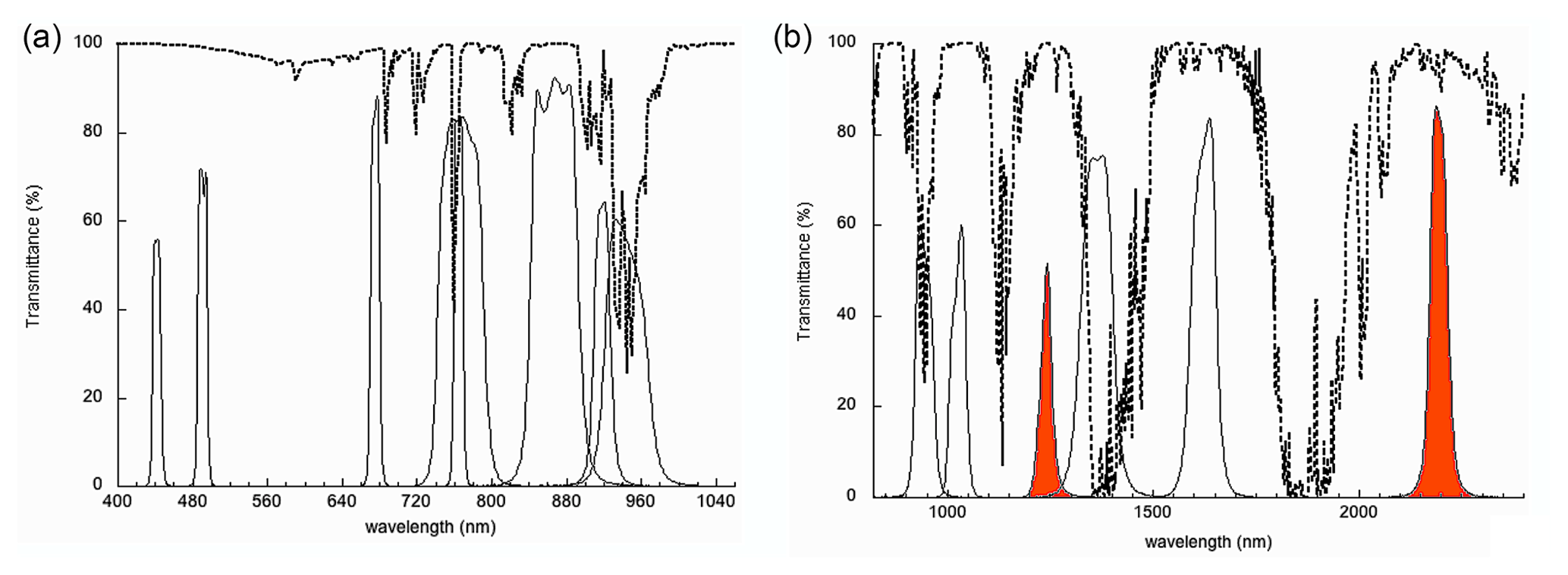
Figure 1Spectral wavelengths of the VIS–NIR (a) and SWIR (b) spectral response function of OSIRIS optical channels without units and normalized to unity. The dashed line corresponds to a typical atmospheric transmittance in percent. The red-colored channels are used in this study (1240 and 2200 nm).
2.1 OSIRIS
OSIRIS (Observing System Including PolaRization in the Solar Infrared Spectrum) is an extended version of the POLDER radiometer (Deschamps et al., 1994) with multi-spectral and polarization capabilities extended to the near-infrared and shortwave infrared. This airborne instrument is a prototype of the future spacecraft 3MI (Marbach et al., 2015) planned to be launched on MetOp-SG in 2024. It consists of two optical sensors, each one with a two-dimensional array of detectors: one for the visible and near-infrared wavelengths (from 440 to 940 nm) named VIS–NIR (Visible–Near-Infrared) and the other one for the near-infrared and shortwave infrared wavelengths (from 940 to 2200 nm) named SWIR (Shortwave Infrared). The VIS–NIR detector contains 1392 pixel × 1040 pixel with a pixel size of 6.45 µm × 6.45 µm, while the SWIR contains 320 pixel × 256 pixel with a pixel size of 30 µm × 30 µm. Adding those characteristics to the wide field of view of both heads, at a typical aircraft height of 10 km, the spatial resolution at the ground is 18 and 58 m for the VIS–NIR and SWIR, respectively. This leads to a swath of about 25 km × 19 km for the visible and 19 km × 15 km for the SWIR.
OSIRIS has eight spectral bands in the VIS–NIR and six in the SWIR. Similar to the concept of POLDER, OSIRIS contains a motorized wheel rotating the filters in front of the detectors. The step-by-step motor allows only one filter to intercept the incoming radiation at a particular wavelength. The polarization measurements are conducted using a second rotating wheel of polarizers. Given the sensor exposure and transfer times, the duration of a full lap is about 7 s for the VIS–NIR and 4 s for the SWIR. Figure 1 shows the spectral response of each channel of OSIRIS. The two channels (1240 and 2200 nm) used in this study are colored red in the figure.
OSIRIS is an imaging radiometer with a wide field of view. It has a sensor matrix that allows the acquisition of images with different viewing angles. The same scene can thus be observed several times during successive acquisitions with variable geometries. The largest dimension of the sensor matrix is oriented along-track of the aircraft to increase the number of viewing angles for the same target. For example, when the airplane is flying at a 10 km altitude with a speed of 200 to 250 m s−1, the same target on the ground can be seen under 20 different angles for the VIS–NIR and 19 for the SWIR.
2.2 Airborne campaign and case study
OSIRIS participated in the airborne campaign CALIOSIRIS in October 2014. It was carried out with the contributions of the French laboratories LOA (Laboratoire d'Optique Atmosphérique) and LATMOS (Laboratoire ATmosphères, Milieux, Observations Spatiales, Paris) and with Safire, the French Facility for Airborne Research. One objective of this campaign was the development of new cloud and aerosol property retrieval algorithms in anticipation of the future space mission of 3MI intending to improve our knowledge of clouds, aerosols, and cloud–aerosol interactions.
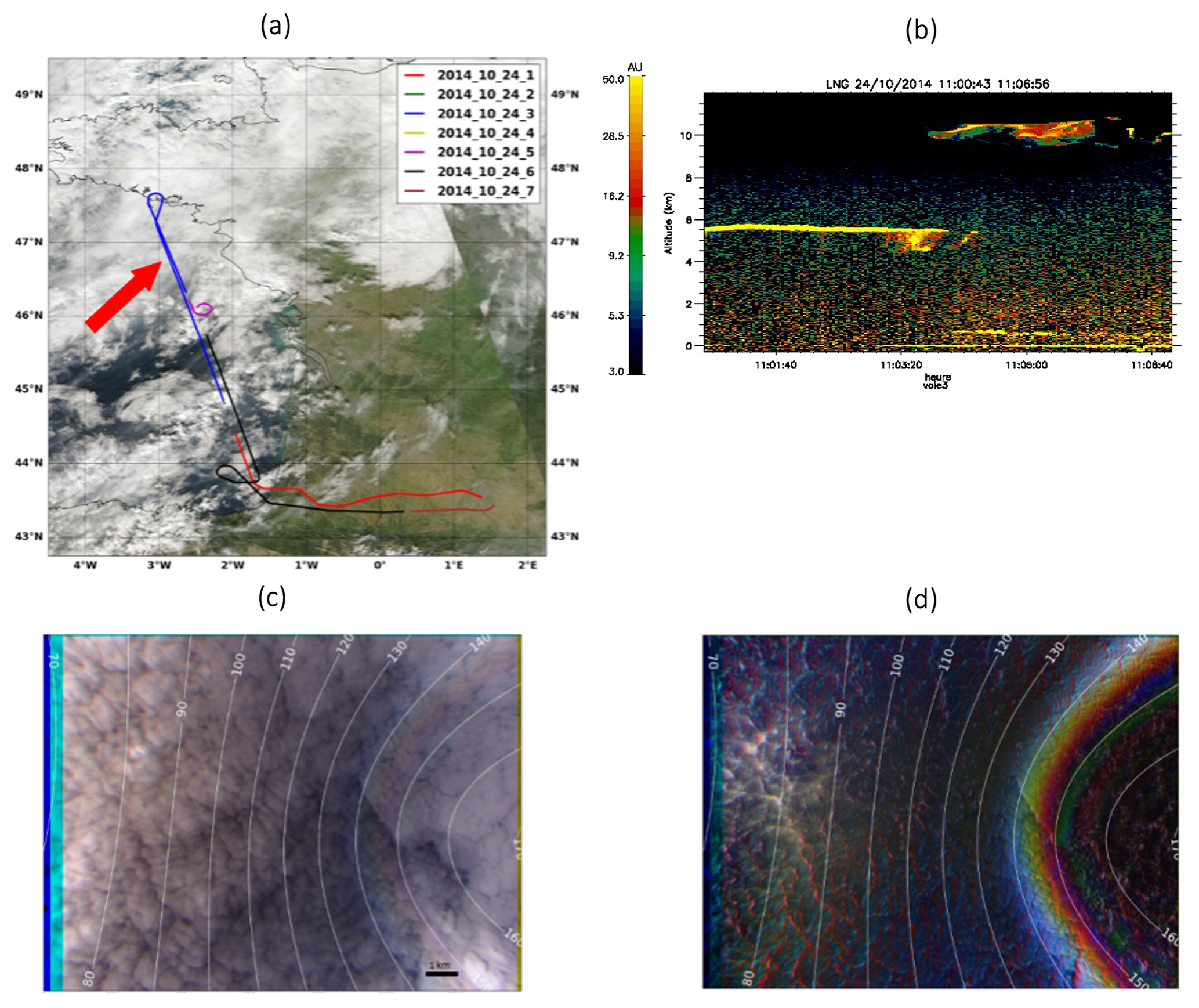
Figure 2Studied case on 24 October 2014 at 09:02 UTC (11:02 LT, local time). (a) In blue is the airplane trajectory for this day above a MODIS/AQUA true color image. The red arrow corresponds to the studied segment. (b) Quick look of the backscattered signal provided by the lidar-LNG around the observed scene. The red rectangle corresponds to the studied scene. (c) OSIRIS RGB composite image obtained from the total radiances at channels 490, 670, and 865 nm. The blue bars on the left-hand side of the images are due to the motion of the airplane between the image acquisitions of the different filters. (d) OSIRIS RGB composite image obtained from the polarized radiances at channels 490, 670, and 865 nm. The white iso-contours in (c) and (d) represent the scattering iso-angles in a 10∘ step.
The data used in this work focus on a cloudy case over the ocean surface: a marine monolayer cloud that was observed on 24 October 2014 at 11:02 LT (local time). The aircraft flew at an altitude of 11 km above the Atlantic Ocean facing the French west coast (46.70∘, −2.82∘, red arrow in Fig. 2a). The solar zenith angle was equal to 59∘. The LNG (lidar aerosols nouvelle generation, Bruneau et al., 2015), a high-spectral-resolution airborne lidar at 355 nm, was also on board the Falcon 20 aircraft along with OSIRIS during the airborne campaign. In Fig. 2b, the vertical profiles of the backscattered signal measured by the lidar-LNG are represented. The red rectangle in Fig. 2b corresponds to OSIRIS images and the scene studied in this paper. The lidar-LNG detected a monolayer cloud around 5.5 km. In Fig. 2c and d, we present colored compositions of total and polarized radiances obtained from three spectral bands of OSIRIS over this cloud scene. One OSIRIS image corresponds to several viewing angles. The zenith angle ranges from about 0∘ in the center of the image to 55∘ in the corner of the image. The white concentric contours represent the scattering iso-angles in a step of 10∘.
The clouds backscatter total solar radiation more intensely in the cloudbow regions near 140∘. The position of the cloudbow peak depends on the wavelength, resulting in the decomposition of the light, which is slightly visible between the 140 and 150∘ scattering angle contours. On the polarized image (Fig. 2d), we observe a stronger directional signature of the signal, characteristic of scattering by spherical droplets showing a cloudbow clearly visible between about 140 and 150∘. At larger scattering angles between 150 and 160∘, we slightly observe the supernumerary bows whose positions vary with the wavelength, alternating between the red, blue, and green channels. The measured polarized signal for scattering angles smaller than 130∘ is largely dominated by molecular scattering at 490 nm, hence the blue color. Since the solar zenith angle is 59∘, the specular direction corresponds to a scattering angle of 62∘ in the solar plane (not visible in Fig. 2c and d), but the ocean wind enlarges the sun glint area, resulting in an enhancement of the radiances between the 70 and 80∘ scattering iso-contours.
At the time of the CALIOSIRIS campaign in 2014, the polarized channels presented calibration and stray light issues, which make use of the polarized measurements difficult for quantitative retrievals. In addition, the images from the two sensors were not well colocated. Consequently, for this work, we use two unpolarized channels of the SWIR matrix, one almost non-absorbing (1240 nm) and one absorbing (2200 nm), to have information on optical thickness and effective radius, respectively.
In order to use the multi-angular capability of OSIRIS, successive images have to be colocated. After subtracting the average of similar successive images to remove the angular effects, the colocation is achieved by minimizing the root mean square difference of the radiances between each pair of successive images for different translations along the line and the column in the second image. The reference image is the central one of the sequence. Images with translations beyond the dimensions of the central image are ignored. Multi-angular radiances at the cloud level correspond in our case to 9 to 13 directions.
One of the most robust approaches in cloud property retrievals is the optimal estimation method (OEM). It is increasingly used in satellite measurement inversion (Cooper et al., 2003; Poulsen et al., 2012; Walther and Heindiger, 2012, Sourdeval et al., 2013; Wang et al., 2016). It provides a rigorous mathematical framework to estimate one or more parameters from different measurements. The OEM also characterizes the uncertainty in the retrieved parameters while taking into account the instrument error and the underlying physical model errors. A complete description of the optimal estimation method for atmospheric applications is given by Clive D. Rodgers (Rodgers, 2000). In this book, Rodgers exhaustively described the information content extraction from measurements, the optimization of the inverse problem, and the solutions and error derivations. In the following, we will go through the basics of this method that define the core of our retrieval algorithm.
3.1 The formalism of the optimal estimation method
Considering a vector y (of dimension ny) containing the measurements and a state vector x (of dimension nx) containing the unknown properties to be retrieved, these two vectors are connected by the forward model F, which can model the complete physics of the measurements to an adequate accuracy. The errors associated with the measurement and the modeling are represented by the error vector ϵ. Equation (1) states the relationship between these variables.
The OEM aims to find the best representation of parameters x that minimizes the difference between simulations F(x) and observations y while considering the linearity of the direct model near the solution. To achieve it, a Bayesian probabilistic approach is applied. Before the measurements, a priori knowledge of the state vector can be described by a probability density function (PDF) P(x). Once the measurements y have been carried out, this knowledge can be described by the posterior PDF of the state P(x|y), which is a conditional probability (probability of having x given that y is true). The posterior PDF of the state vector can be related to its a priori PDF by Bayes' theorem:
where P(y) is the PDF of the measurements including the uncertainties and P(y|x) is the PDF of the measurements given that we know the state vector.
In the optimal estimation method, the previous PDFs are represented by Gaussian distributions, assuming that the errors of the measurements, the errors related to the non-retrieved parameters, and the errors of the forward model are normally distributed around a mean value.
Therefore, it can be easily shown that the best estimate of the state vector x corresponds to the minimum of the so-called cost function J(x).
The first term of J(x) represents the difference between the measurements and the forward model calculated for a given state vector x weighted by Sϵ, the covariance matrix associated with the measurement error and the forward model errors. The second term represents the difference between the state vector x and the a priori state vector xa weighted by Sa, the covariance matrix associated with xa. In line with the cost function, the optimal estimation emerges from a balance between the information carried by the measurement about the state vector and what we already know about it before the measurement. In our case, we do not have a prior estimate of the state vector. The iterations are initiated by a first guess while applying a large Sa. The difference between the measurements and the forward model will be the decisive element in the minimization of the cost function. It will ensure that the estimated cloud properties have the optimal fit with the observed system only.
The minimization is done through the Levenberg–Marquardt approach (Marquardt, 1963; Levenberg, 1944) based on the “Gauss–Newton” iterative method. Assuming the model is nearly linear around a given state vector, each iteration is calculated following Eq. (4):
where xi is the state vector at the ith iteration, Ki is the sensitivity (or Jacobian) matrix described in Eq. (10), and is the covariance matrix of the state vector defined in Eq. (5).
The parameter γ affects the size of the step at each iteration. If the cost function increases at an iterative step i then γ is increased and a new smaller step (xi+1) is calculated until the cost function decreases.
The iterative process stops when the simulation fits the measurement (Eq. 6), named convergence of Type 1, or when the iteration converges (Eq. 7), named convergence of Type 2. The left side of Eq. (6) represents the normalized cost function without taking into account the a priori negligible contribution. When the cost function is smaller than ny or the normalized cost function () is less than or equal to 1, the iterations stop. Equation (7) deals with the iterative steps and will make sure that the iterations will stop when the difference between two successive steps weighed by Sx is less than nx: in other words, when further changes in the state vector have small to zero changes in the minimization.
When neither the inequality of Eq. (6) nor the inequality of Eq. (7) is reached after 15 iterations, the retrieval is considered a failed retrieval.
3.2 Basic setting of the retrieval algorithm
In order to apply this theoretical framework to our retrieval algorithm, we next define the basic elements stated in the previous subsection.
The state vector x contains the properties to be retrieved. In our case, they are the cloud optical thickness (COT) and the effective radius of water droplets (Reff).
It can be noted that because the relationship between radiances and optical thickness has a logarithmic shape, using log(COT) instead of COT in the state vector could have accelerated the convergence.
The a priori state vector was set to [10, 10 µm] and the a priori covariance matrix Sa was set to 108. The latter was to be chosen very large to favor the measurements in the determination of the state vector (no a priori constraint).
The measurement vector y contains the radiances (R) measured by OSIRIS at two wavelengths λa and λb for several view directions θi and is given in Eq. (9).
The forward model is based on the adding–doubling method (De Haan et al., 1987; Van de Hulst, 1963) to solve the radiative transfer equation and simulate the radiances measured by OSIRIS for the corresponding observation geometries and wavelengths. It is a major element of the retrieval and describes the radiation interaction with the cloud, the surface, and the atmosphere while fixing several parameters (e.g., wind speed, cloud altitude). We assume a standard atmosphere with a midlatitude summer McClatchey profile (McClatchey et al., 1972) for the computation of molecular scattering. As the two channels used in the retrieval are in atmospheric windows (as seen in Fig. 1), the atmospheric absorption is not accounted for. It is not completely true, and therefore the cloud optical thickness will be slightly underestimated and the effective radius slightly overestimated. Our case study is purely above an ocean surface. The reflection by the surface can affect the measured radiances even in cloudy conditions and particularly for optically thin clouds. The anisotropic surface reflectance of the ocean surface is characterized by a bidirectional polarization distribution function (BPDF). We used the well-known Cox and Munk model to compute the specular reflection modulated by ocean waves (Cox and Munk, 1954) with a fixed ocean wind speed based on the NCEP reanalysis of the National Oceanic and Atmospheric Administration (NOAA).
As in current operational algorithms, the cloud model used for the retrieval is a plane-parallel and homogeneous (PPH) cloud, which implies the independent pixel approximation (IPA). The case study is a liquid water cloud scene. Therefore, we used a lognormal distribution for the size of particles, which are assumed to be spherical (Hansen and Travis, 1974) and described by an effective radius and an effective variance (veff). The altitude of the cloud is determined by the measurements of the lidar-LNG that was on board the research aircraft Safire Falcon 20 during the airborne campaign. All simulations are monochromatic computations at the central wavelength of OSIRIS channels. The altitude of OSIRIS and the illumination and observation geometries are calculated based on the coordinates of the aircraft inertial unit.
The Jacobian matrix K includes the partial derivatives of the forward model to each element of the state vector (Eq. 10). The columns of K then define the sensitivity of the radiances (each with a specific wavelength – viewing angle configuration) to COT or Reff. The rows of the Jacobian define the sensitivity of each radiance configuration to the two retrieved properties. The Jacobian matrix is computed using finite differences.
3.3 Error characterization
During the retrieval process, every element is associated with a random or systematic error embedded in the error covariance matrix Sϵ. The account of errors in the inverse problem does not allow a unique value for the solution x but instead a Gaussian probability distribution function (PDF), where x is the expected value and Sx is its covariance.
Sx is calculated after a successful convergence with Eq. (4) using the Jacobian at the retrieved state and Sϵ. This posterior variance–covariance matrix can also be written as follows.
In this formulation, we have assumed that the two terms of the state vector are independent, and thus the off-diagonal terms of Sx are assumed to be zero. The use of Gaussian PDFs leads to computing the uncertainty in a particular parameter xk as the square root of the corresponding diagonal elements of the covariance matrix , where k is the index of the parameter in the state vector x (Eq. 11). We chose to express this uncertainty using the relative standard deviation (RSD) in percent (Eq. 12). The RSD will be used to characterize the quality of the retrieval.
Sϵ represents the sum of the measurement (Smes) and forward model variance–covariance matrix. Indeed, the forward model F uses ancillary information provided by a set of fixed parameters b (listed in Sect. 3.3.2). Errors related to an uncertain estimation of these fixed parameters are represented by the covariance matrix Sfp described in the next section.
Besides the fixed parameters, the cloud model used in the radiative transfer computation can also be a source of uncertainty. The uncertainties of the retrieved parameters related to this approximation are regrouped in the covariance matrix SF described in the next section. Sϵ is then addressed as a sum of these three components:
Previous studies (Wang et al., 2016; Iwabuchi et al., 2016; Poulsen et al., 2012; Sourdeval et al., 2015) have already computed and presented the uncertainties of the retrieved cloud properties for all error contributions using Sϵ. Further, Walther and Heidinger (2012) use the optimal estimation framework to separate the contribution of measurement errors and several non-retrieved parameters. In our work, a similar framework was used to separate the contribution of each type of uncertainty also including the forward model uncertainties. The aim is to better quantify and understand the limitation of using a simplified forward model in such a cloud retrieval algorithm. It is realized by propagating the covariance matrices of errors from the measurement space into the retrieved state space (Rodgers, 2000). The gain matrix Gy, which represents the sensitivity of the retrieved quantities to the measurement, is then used:
The total variance–covariance matrix of the retrieved state vector (Sx) can then be decomposed into three contributions (Eq. 15), with each term originating from its corresponding error covariance matrix.
Each term in this equation is developed and discussed in the following three subsections.
3.3.1 Uncertainties related to the measurements
Any type of measurement is subject to errors. It is necessary to apply calibration processes to study the relationship between the electrical signals measured by the detectors and the radiances and quantify its uncertainty. Calibration is done during laboratory experiments before the airborne campaign or the instrument launch into space (Hickey and Karoli, 1974). It can be done in situ if calibration sources are available on board the sensor (Elsaesser and Kummerow, 2008) or it can be vicarious (e.g., Hagolle et al., 1999) by using natural or artificial sites on the surface of the Earth. The uncertainties of the measurements remaining after the calibration processes are assumed, random, and uncorrelated between channels and can be consistently approximated by a Gaussian probability density function over the measurement space.
As errors between measurements are supposed to be independent, the covariance matrix of measurement noise (Smes) is diagonal with dimensions equal to the measurement vector dimension (ny×ny). The diagonal elements are the square of the standard deviation of the measurement errors. In our retrievals, we calculated the covariance matrix based on 5 % of measurement errors: .
The error covariance matrix for the retrieved parameters due to measurement errors is then expressed by mapping the covariance matrix Smes from the measurement space to the state space by using the gain matrix Gy:
The uncertainty in a particular parameter xk originating from the measurement errors is defined as the square root of the corresponding diagonal element corresponding to the standard deviation . It is expressed using the RSD (mes) as in Eq. (12).
3.3.2 Uncertainties related to the fixed parameters
Any retrievals from remote sensing observations require prior knowledge of several unknown parameters used in the forward model computation. Those parameters are not retrieved due to a lack of sufficient information. To compute the fixed parameters (fp) errors, we quantified the possible error in our estimation of the fixed model parameters. In our case study, these parameters are the altitude of the cloud (alt), the effective variance of the cloud droplet size distribution (veff), and the ocean wind speed (ws). These errors are considered to be independent and random under the assumption of linearity of the radiances around the fixed parameters. They are set in the diagonal covariance matrix Sσfp. They are weighed by Kfp, the Jacobian matrix containing the gradient of the forward model with respect to the fixed parameters. Finally, as previously, the errors are mapped from the measurement space to the state vector space through Gy to estimate their contribution to the retrieval uncertainty as follows.
Each column in Kfp and Sσfp is dedicated to one fixed parameter. Therefore, we can separate the contributions of every element of the fixed parameters vector as follows.
Each covariance matrix from the right side of Eq. (19) is developed as shown in Eq. (20). is the standard deviation of the fixed parameter error and is a column vector containing the gradient of the forward model with regard to the same fixed parameter bi.
In order to develop for each element of b, the forward model has been constructed in a flexible way that permits initiating small variations of any fixed parameter and then calculating the partial derivatives of the forward model with regard to the ancillary data, called the Jacobians of the fixed parameters Kalt, , and Kws.
The last elements needed to resolve Eq. (20) are the errors or standard deviations of the cloud altitude, the effective variance of water droplets, and the ocean wind speed: σalt, , and σws, respectively.
The values and the uncertainties of these fixed parameters are chosen according to the experimental setup of the campaign. To estimate the uncertainties originating from the fixed cloud altitude, we used the opportunity of having the lidar-LNG aboard the aircraft, which gives the backscattering signal obtained around the case study of CALIOSIRIS. From 11:01:06 to 11:03:06 CEST (the time when the same cloud scene is apparent), the cloud altitude varies between 5.57 and 5.73 km in our cloud scene. For practical reasons related to the radiative transfer code, we use a value of 6 km for the cloud-top altitude and a standard deviation of σalt = 0.16 km (3 % of the cloud altitude). This value is low thanks to the knowledge provided by the lidar.
Concerning the effective variance veff, to which the polarized radiance is highly sensitive in the supernumerary arcs near the cloudbow (Bréon and Goloub, 1998), we fixed a value of 0.02 based on the number of supernumerary bows in the polarized radiances (not shown). After simulating radiances with several values of veff, we choose to add a = 0.003(15 %) possible error in the estimation of this parameter. As the value of veff was fixed using the polarization measurements of OSIRIS, this uncertainty is weak and not representative of all situations.
For the ocean wind speed fixed to 8 m s−1 obtained from the database of the National Oceanic and Atmospheric Administration, we used an error σws = 0.8 m s−1 (10 %). It covers the possible sources of error in surface wind speed retrievals.
3.3.3 Uncertainties related to the forward model
Forward models are usually formulated around some limitations and assumptions that can contribute to the uncertainty of the retrieved parameters. The forward model used to simulate the radiances measured by OSIRIS follows the cloud plane-parallel assumption. This assumption is known to cause errors in the retrieved parameters (see Sect. 1) that can be assessed and included in the total uncertainty. The evaluation of these modeling errors requires an alternative forward model F′ that includes more realistic physics. The contribution of this error is represented by the following equation.
SF is diagonal with dimensions equal to the measurement vector dimensions (ny×ny). Each diagonal element is the square of the difference between radiance computed for a specific direction with the simplified forward model F and the one computed with the more realistic forward model F′ while maintaining the same state vector and the same fixed parameter vector b: .
The simplified model used for the retrieval can lead to biased retrieved parameters. In this case, the bias due to the model will be included in the Gaussian PDF width, resulting in an overestimation of the uncertainties.
The uncertainties related to the cloud vertical homogeneity and the cloud horizontal homogeneity are quantified separately. In the following, we present the elements of the forward model used to quantify the uncertainties of these assumptions.
Nonuniform cloud vertical profile model
The vertically heterogeneous cloud model to assess the uncertainties of the assumed homogeneous cloud model is described by
-
an effective radius profile and possibly an effective variance profile but for simplification – we will consider veff to be constant over the entire vertical profile with a value of 0.02;
-
an extinction coefficient (σext) profile; and
-
a cloud geometrical thickness (CGT) characterized by the difference between the altitude of the cloud top (ztop) and the cloud base (zbot). The values of CGT, ztop, and zbot are fixed based on the lidar measurements.
The effective radius and extinction coefficient profiles are computed using an analytical model already introduced in Merlin (2016). It is based on adiabatic cloud profiles, which are described and used in several studies (Chang, 2002; Kokhanovsky and Rozanov, 2012). In the adiabatic scheme, the effective radius increases with altitude. However, several studies proved that a simple adiabatic profile is not sufficient to describe a realistic cloud profile (Platnick, 2000; Seethala and Horváth, 2010; Nakajima et al., 2010; Miller et al., 2016). Depending on the maturity of the cloud, turbulent and evaporation processes can reduce the size of droplets at the top of the cloud and/or collision and coalescence processes can increase the size of the droplets in the lower part of the clouds as observed by Doppler radar (Kollias et al., 2011). The profile used in this study aims to represent the case of droplet size reduction at the top of the cloud, but other and more sophisticated and representative profiles can be used (Saito et al., 2019).
The description of this more realistic vertical cloud profile is obtained with two adiabatic profiles (Fig. 3) that are joined at the altitude of maximum liquid water content (LWC) called zmax.
-
The first profile from zbot to zmax is considered adiabatic.
-
The second profile from zmax to ztop follows an adiabatic LWC profile decreasing with altitude.
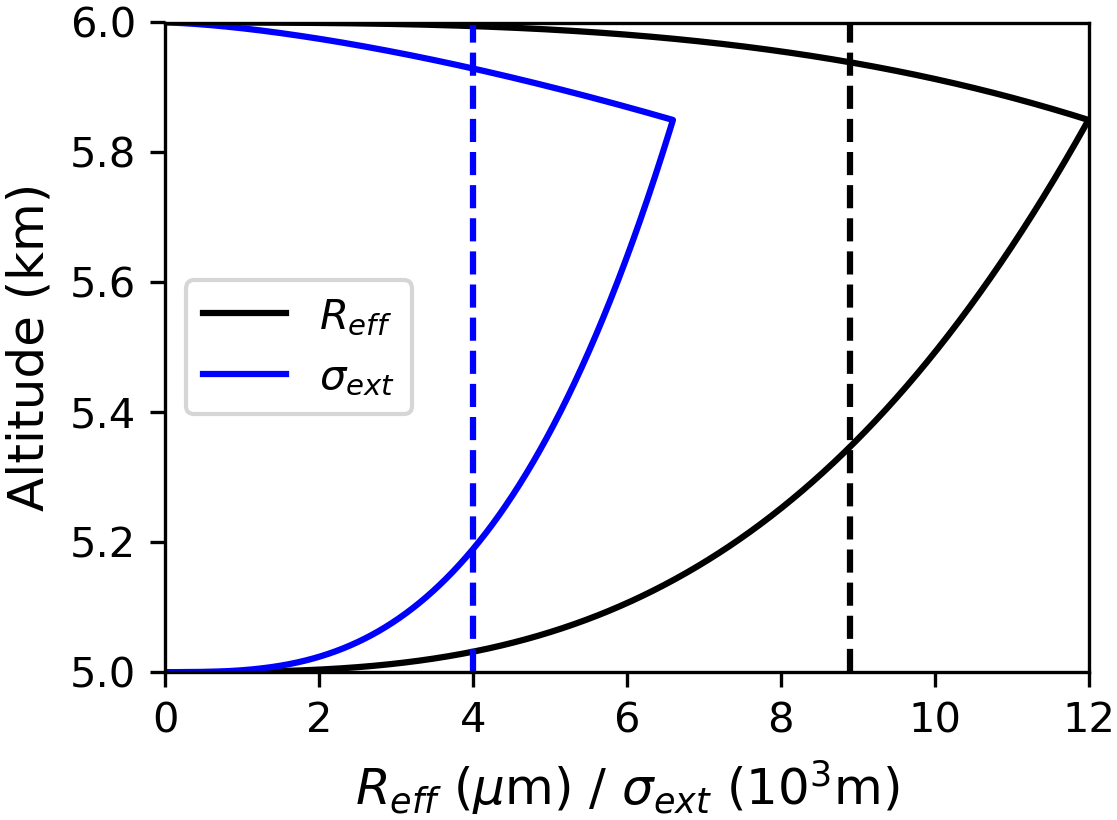
Figure 3The heterogeneous vertical profile of effective radius (black line) and extinction coefficient (blue line) used to assess uncertainties due to the assumption used for the vertical profile. The equivalent homogeneous vertical profiles are shown in dashed lines. The cloud is between 5 and 6 km. The maximum extinction coefficient and effective radius are 6.6 km−1 and 12 µm, respectively, and the altitude zmax is 5.85 km.
Considering that LWC is equal to zero at the base and top of the cloud and relying on the linear variation model of the LWC with altitude (z) established in Platnick (2000), we can write the following.
The profiles of effective radius (Eq. 23) and extinction coefficient (Eq. 24) can then be computed by considering that the particle concentration is constant over the entire cloud, which makes it possible to obtain analytical functions of LWC, Reff, and σext.
A form factor p (Eq. 25) allows the adjustment of the altitude zmax, where the extinction coefficient and the effective radius are the largest:
This unitless parameter p varies from 0 to 1, representing the shape of the profile. The value 0 corresponds to zmax=ztop (adiabatic cloud) and the value 1 corresponds to zmax=zbot (a reverse adiabatic cloud with a negative gradient of water content). In the following results, a value of 0.15 is assigned to this parameter which, allows having a profile close to the one studied in Miller et al. (2016) from large eddy simulation (LES) cloud scenes.
To assess the error due to the vertical heterogeneity of the cloud, we need to specify the maximum value of the extinction coefficient and the effective radius of the vertically heterogeneous cloud corresponding to the “equivalent” homogeneous clouds. Several options are possible for these values. We choose to use Eq. (26) to assign , which leads to the same integrated extinction profile, and Eq. (27) to assign to ensure that the mean Reff of the heterogeneous vertical profile is equal to the Reff of the homogeneous cloud (). and are found analytically by integrating the profiles described in Eqs. (23) and (24).
A vertically heterogeneous cloud is computed for each pixel using the retrieved value based on the homogeneous assumption. The error covariance matrix describing the error due to the simple homogenous cloud assumption (Eq. 21) is calculated from the difference between radiances computed with homogeneous and heterogeneous vertical profiles, denoted F and F′, respectively.
The 3D radiative transfer model
The other assumption that might affect the retrieved cloud optical properties in the current operational algorithms is the horizontally plane-parallel and homogeneous (PPH) assumption for each observed pixel. It implies that each pixel is horizontally homogeneous and independent of the neighboring pixels, known as the independent pixel approximation (IPA). The homogeneous PPH assumption affects the cloud-top radiances and leads to differences between 1D and 3D radiances that are the result of several effects discussed in numerous publications and briefly summarized in Sect. 1. This PPH assumption includes errors known as the PPH bias due to the subpixel variations of the cloud and errors related to the photon horizontal transport between columns (IPA error). At the high spatial resolution of OSIRIS (less than 50 m), it was shown from airborne data that the dominating effect is related to the IPA error (Zinner et Mayer, 2006). In the following, we thus consider only this error and assume that the pixel is homogeneous at the measurement scale.
To assess the uncertainties in the retrievals arising from this assumption, Eq. (21) is used. SF is then the difference between the radiances computed with a 1D radiative transfer code (1D-RT), following the adding–doubling method (Hansen and Travis, 1974), and the radiances computed with a 3D radiative transfer (3D-RT) code called 3DMCPOL (Cornet et al., 2010). The 3D simulations use, for each pixel, the COT and Reff retrieved using the PPH assumption. Errors in cloud model assumptions are assessed independently, so a vertical homogeneous profile is assumed. We also assume a flat cloud top, which leads to underestimated differences and errors as cloud-top variation may increase the differences between 3D and 1D radiances (Várnai and Davies, 1999; Várnai, 2000). The differences are thus mainly due to the lateral photon transport, which tends to smooth the radiances fields compared to their 1D counterpart (Davis et al., 1997) and to the cloud heterogeneity along the line of sight (e.g., Fauchez et al., 2018).
Our strategy to assess the different types of uncertainty follows two steps. In a first step, we retrieve COT and Reff using a bispectral multi-angular method by considering the uncertainties related to the measurement errors alone. We use a weakly absorbing channel centered at 1240 nm that is mainly sensitive to COT and a partially absorbing channel centered at 2200 nm that is thus sensitive to Reff. In this case study, up to 13 viewing angles are available for each pixel. In the first step, only the measurement errors are accounted for and included in Sϵ. This error is usually well characterized and does not change once the measurements are realized. Not considering the other errors at this stage allows benefiting from a faster retrieval algorithm without the calculation of Kb and the heavy computation cost of heterogeneous cloud profiles and 3D-RT calculations. The second step consists of computing the errors due the non-retrieved parameters and due to the assumption of a vertically and horizontally homogeneous cloud for the retrieval of Reff and COT.
It should be noted that the parameters retrieved in the first step may be biased, in particular due to the use of a simplified cloud model to connect the state vector to the measurements. We assume that the estimation of the uncertainties performed in the second step is, however, correct if the variations predicted by the simplified and the realistic models around the retrieved values (potentially biased) and around the true values are identical. This is correct with a linear forward model but can be an assumption that is too strong in cloud retrieval regarding the nonlinearity of the relationship of the radiances as a function of cloud parameters. A way to test this assumption would be to use numerical experiments.
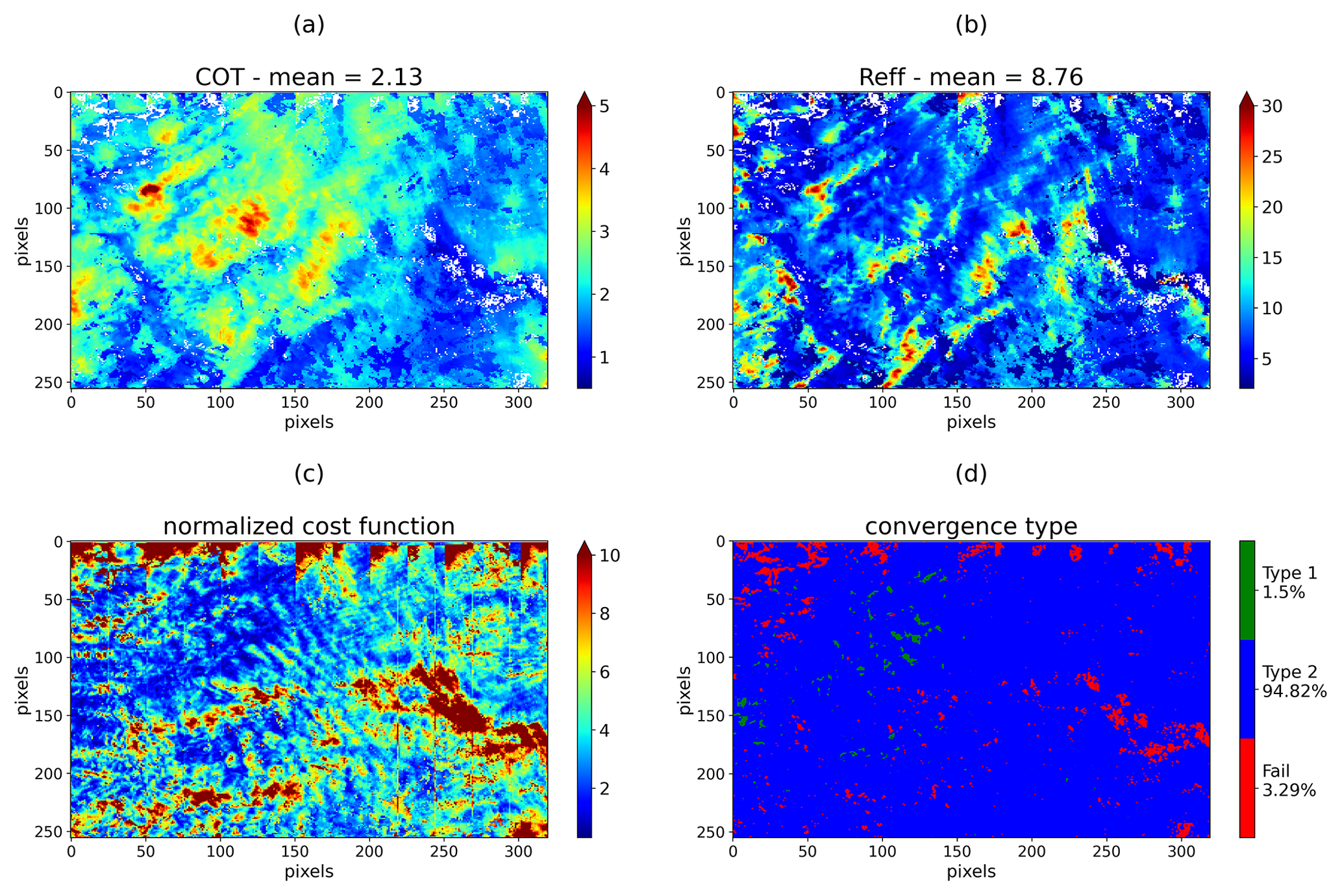
Figure 4COT (a) and Reff (b) retrieved using a multi-angular bispectral method from a liquid cloud case observed during the CALIOSIRIS airborne campaign on 24 October 2014 at 11:02 LT (local time). Pixels associated with failed retrievals are represented by white pixels. (c) Normalized cost function. (d) Convergence type (Eq. 6 for Type 1 and Eq. 7 for Type 2) and failed retrieval.
In Fig. 4, COT (Fig. 4a) and Reff (Fig. 4b) retrieved from multi-angular SWIR radiances are presented. Spatial variations are mainly due to variations in the observed cloud structures. The COT range is between 0.5 and 6 with a mean value of 2.1. Some values of COT are very small, but no clear-sky pixel is present. Reff varies between 2 and 24 µm around a mean value of 8.8 µm. Figure 4c presents the normalized cost function, which is less than or equal to 1 when the retrieval successfully converges according to Eq. (6) (convergence of Type 1). In the case of multi-angular measurements, the normalized cost function is often above 1, meaning that the simulated radiances do not fit the measurements while considering the measurement error covariance only. This comes from the attempt to fit the measured radiances from all the available viewing directions with a simple forward model, which is far from reality. The retrieval thus stops mainly according to Eq. (7) (convergence of Type 2), indicating that the state vector remains almost constant between two successive iterations. When neither Eq. (6) nor Eq. (7) is achieved, the retrieval fails. For the whole scene, failed retrievals account for 3.3 % of the pixels. The failure may be associated with pairs of radiances outside the LUT that can occur for several reasons that are well documented in Cho et al. (2015).
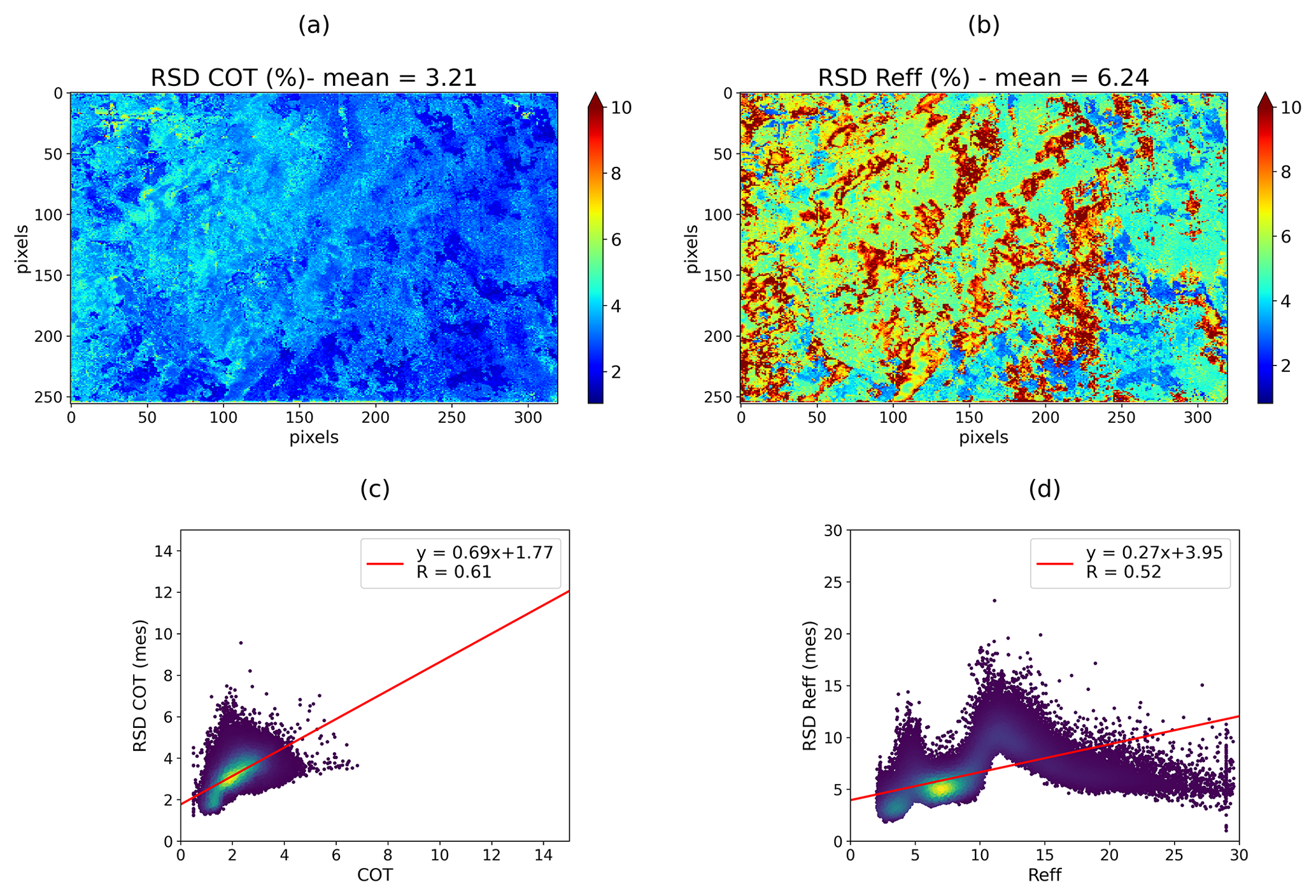
Figure 5Uncertainties (RSD) in percent for COT (a) and Reff (b) originating from the measurement errors for the case study of CALIOSIRIS. COT uncertainties as a function of COT (c). Reff uncertainties as a function of Reff (d).
As detailed in Sect. 3.3, the final error is divided into three categories. Figure 5 shows the uncertainties originating from a 5 % measurement error in the retrieved COT, RSD COT (mes), and in the retrieved Reff, RSD Reff (mes). RSD COT (mes) ranges from 0.5 % to 5 % with a mean value of 3.2 %, while RSD Reff (mes) ranges from 2 % to 12 % with a mean value equal to 6.3 %. These uncertainties are plotted according to their respective values in Fig. 5c and d. RSD COT (mes) increases with the magnitude of the retrieved COT, as RSD Reff (mes) tends to do with Reff for values until 12 µm. The uncertainties due to measurement errors are low, especially for optical thickness (less than 5 %). This is related to the quasi-linearity and the steep slope of the radiance as a function of COT in this cloud regime (small COT). When the radiance–COT relationship is quasi-linear, the sensitivity of the forward model to COT is high, which consequently leads to parameters retrieved with a high accuracy (low RSD). When COT increases, the gradient of the radiance–COT relationship decreases, causing larger uncertainties.
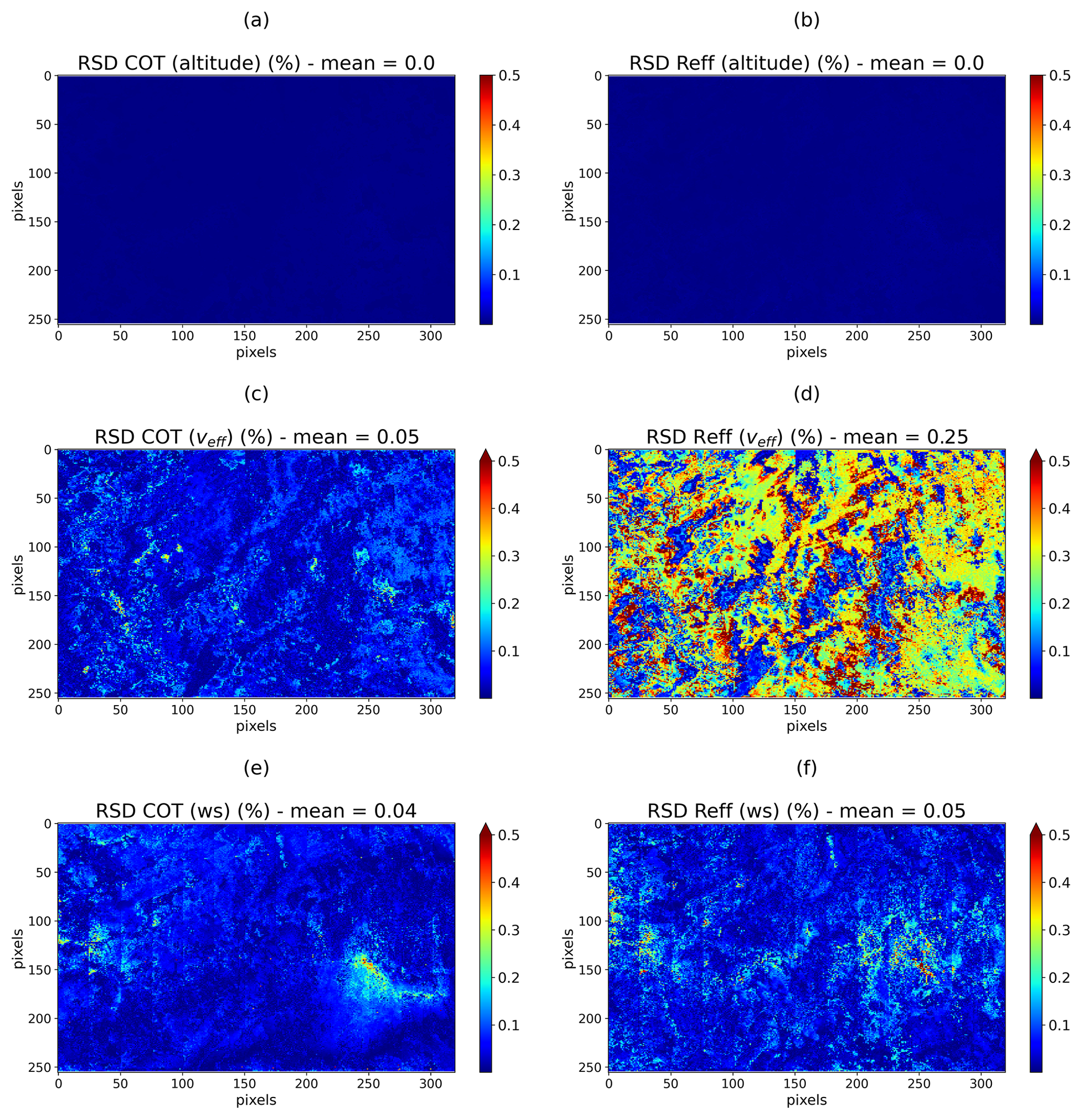
Figure 6The uncertainty RSD (%) of COT (left column; a, c, and e) and Reff (right column; b, d, and f) originating from the non-retrieved parameter errors: altitude (a, b), the effective variance of water droplet distribution (c, d), and the surface wind speed (e, f).
The second type of uncertainty is related to the fixed parameters in the forward model. In Fig. 6, we show the uncertainty in COT and Reff in percent due to an incorrect estimation of each fixed parameter in the forward model. Figure 6a and b represent the uncertainties originating from the fixed cloud altitude, RSD COT (alt) and RSD Reff (alt), respectively. Both show very small uncertainties with values close to zero. In fact, in the visible range, the altitude of the cloud mainly determined the amount of Rayleigh scattering that occurs above the cloud. This type of scattering is dominant at shorter and visible wavelengths and becomes negligible at the studied wavelengths (1240 and 2200 nm). Consequently, at these wavelengths, an error in the fixed cloud altitude does not contribute to the uncertainty in the retrieved COT and Reff.
Figure 6c and d represent the uncertainties of the retrieved COT and Reff originating from the fixed effective variance of the particle size distribution. They are nearly null in COT with a mean value of 0.05 %, as the 15 % uncertainty in the value of veff (0.02) does not modify the total radiances. On the other hand, RSD Reff (veff) reaches 0.5 % with a mean value of 0.25 %. Indeed, veff modifies the width of the cloud droplet distribution and consequently slightly modifies the absorption by cloud droplets, resulting in a larger error. For Reff higher than 15 µm, the relationship between SWIR radiances and Reff tends to flatten, which makes them less sensitive to veff, and thus the uncertainties are smaller than 0.1 %. We remind the reader that we fixed the value of veff using multi-angular polarized measurements of OSIRIS, which leads to the choice of a weak uncertainty for veff (15 %). In the case of a lack of information on veff in the measurements, the uncertainty should be higher, and thus there are errors due to the non-retrieved effective variance. Platnick et al. (2017) obtain 2 % and 4 % uncertainty for COT and Reff, respectively, for veff ranging between 0.05 and 0.2.
Figure 6e and f show that an error in the estimation of the ocean wind speed affects the retrieved COT and Reff mainly for small COT. The water–air interface is reflected mainly in the specular direction, but the ocean being not perfectly smooth, the bright surface (named glitter) is enlarged by the waves formed by the wind. The higher the surface wind speed is, the greater the amplitude of the waves is, leading to a larger reflection angle (wider sun glint). The sun glint reflection is seen by OSIRIS only for very small values of COT and implies uncertainties of the retrieved parameters of about 0.5 %. In the case of broken clouds, the errors resulting from the ocean wind speed uncertainties would be larger. At higher COT, the surface is non-apparent to OSIRIS measurements, and uncertainties are thus close to zero.
We note that all the uncertainties of the studied fixed parameters remain below 1 %, which shows that retrieval of all the COT–Reff couples does not have a high dependence on the fixed forward model parameters.
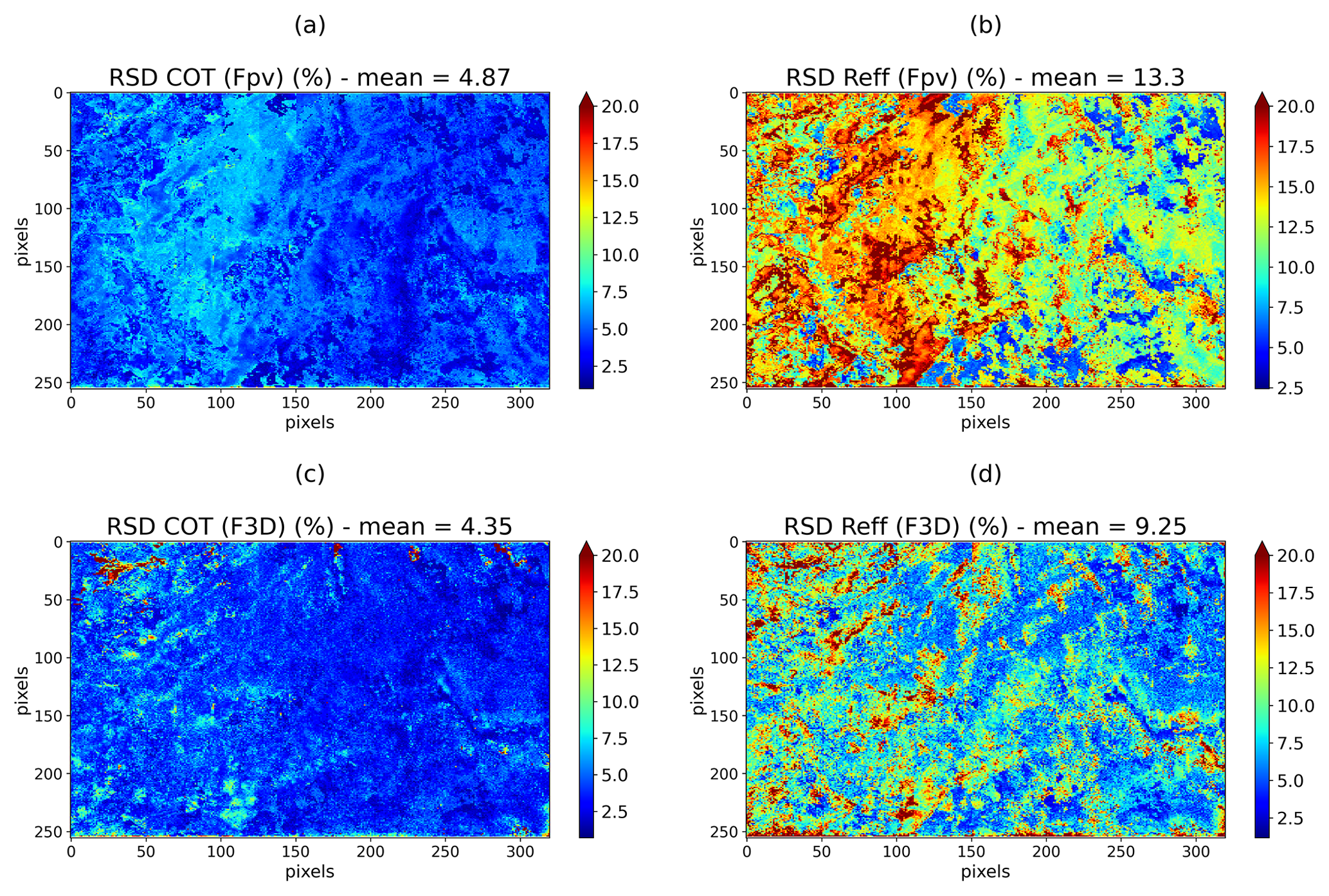
Figure 7The uncertainties (%) in COT and Reff originating from the assumptions in the forward model when not considering the heterogeneous vertical profile (a, b) and the 3D radiative transfer (c, d).
The uncertainties due to the assumptions of the forward model are presented in Fig. 7. Figure 7a and b represent the uncertainties of COT and Reff, respectively, originating from the vertically homogeneous assumption. RSD COT (Fpv) ranges between 1 % and 8 % with a mean value of 4.9 %, while RSD Reff (Fpv) varies from 2 % to 20 % with a mean value of 13.3 %. We note that when the cloud is optically thin (left part of the image), RSD COT (Fpv) and RSD Reff (Fpv) tend to be lower. When the extinction is small, the radiation penetrates deeper into the cloud and brings information on the whole cloud, similar to the one obtained with the homogenous vertical profile. The differences between radiances coming from the vertical heterogeneous and homogeneous profiles are thus small since the integrated extinction over the cloud is approximately the same in both cases. For larger COT, the radiation penetrates less in the cloud and is only affected by the upper part of the cloud where the extinction coefficient is different from one profile to another. In this case, RSD COT (Fpv) and RSD Reff (Fpv) are larger at up to 8 % and 20 %, respectively.
The uncertainties originating from the use of a 1D radiative transfer code instead of a more realistic 3D radiative transfer are represented in Fig. 7c and d for COT and Reff, respectively. RSD COT (F3D) ranges between 1 % and 20 % with a mean value of 4.35 %, while RSD Reff (F3D) varies from 2 % to 18 % with a mean value of 9.25 %. We remind the reader here that, given the high spatial resolution of OSIRIS measurements, we consider the PPH bias to be negligible and do not account for the subpixel variability of cloud properties in the 3D radiative transfer simulation.
Considering the solar zenith incidence angle (59∘), illumination and shadowing effects can also be present depending on the viewing geometries and roughness of the radiative fields (Varnai, 2000). However, in this work, we are dealing with flat cloud tops that induce weaker 3D effects than bumpy cloud tops (Varnai et Davies, 1999). In addition, with multi-angular measurements, the same cloudy pixel is viewed under different viewing angles, which may tend to mitigate the influence of illumination and shadowing effects.
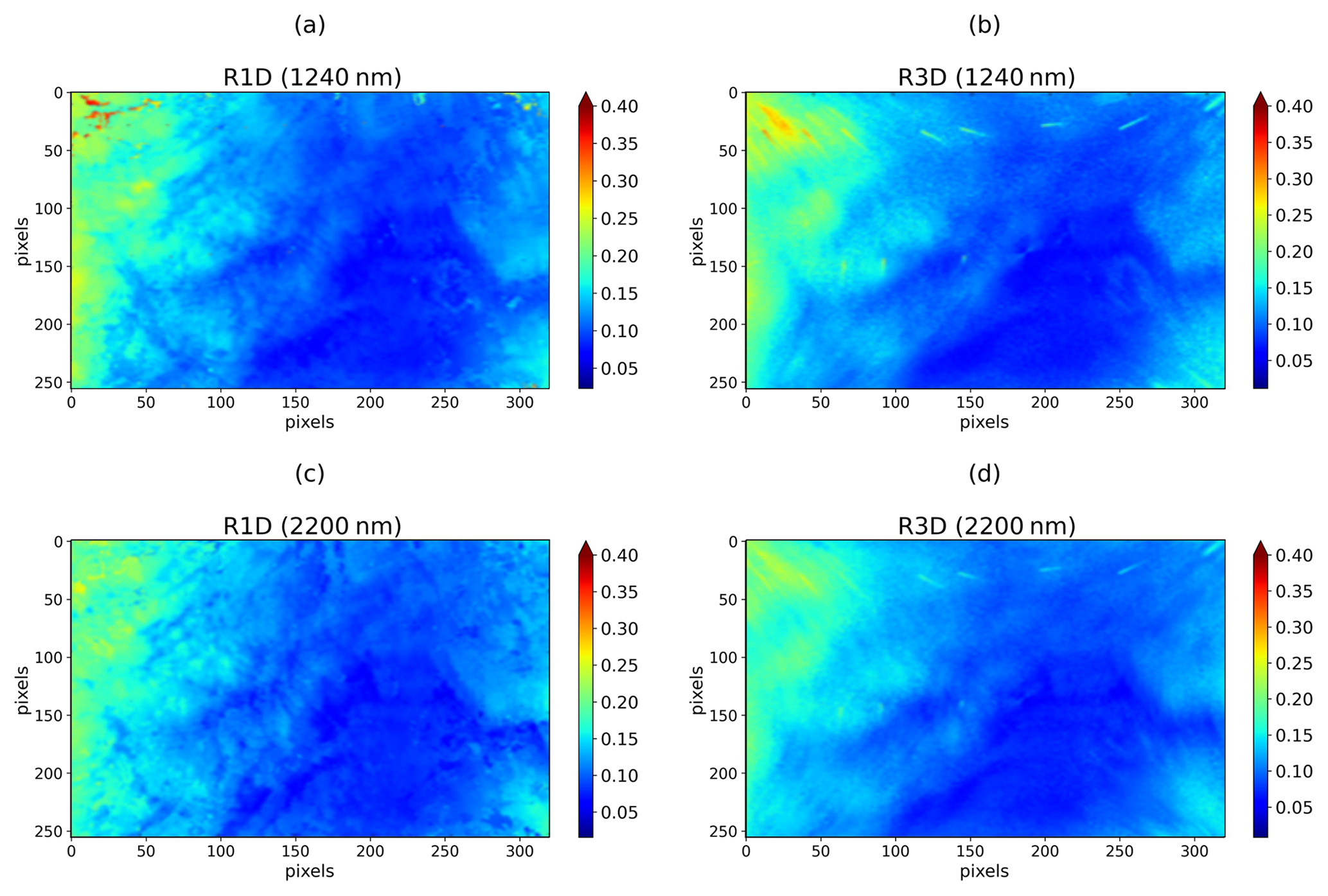
Figure 8The simulated 1D (a) and 3D (b) reflectances at 1240 nm using the retrieved COT and Reff presented in Fig. 4 for the central image. Panels (c) and (d) are the same as (a) and (b) but for 2200 nm.
At this scale, the effects related to the independent pixel approximation (IPA) (Oreopoulos and Davies, 1998) are dominant since the horizontal transfers of photons between pixels are important. The smaller the column horizontal sizes that are considered, the more the real behavior of radiation in the atmosphere will be misrepresented. The horizontal radiation transport (HRT) tends to smooth the radiative field by increasing or decreasing the radiances according to the optical thickness gradient between the considered pixel and its neighbors. This effect is shown in Fig. 8. Figure 8b and d, representing the reflectances computed with 3DMCPOL at 1240 and 2200 nm, respectively show the smoothest field compared to the reflectances computed with a 1D radiative transfer model in Fig. 8a and c. The variabilities in the 3D radiative field are indeed less pronounced compared to the 1D field.
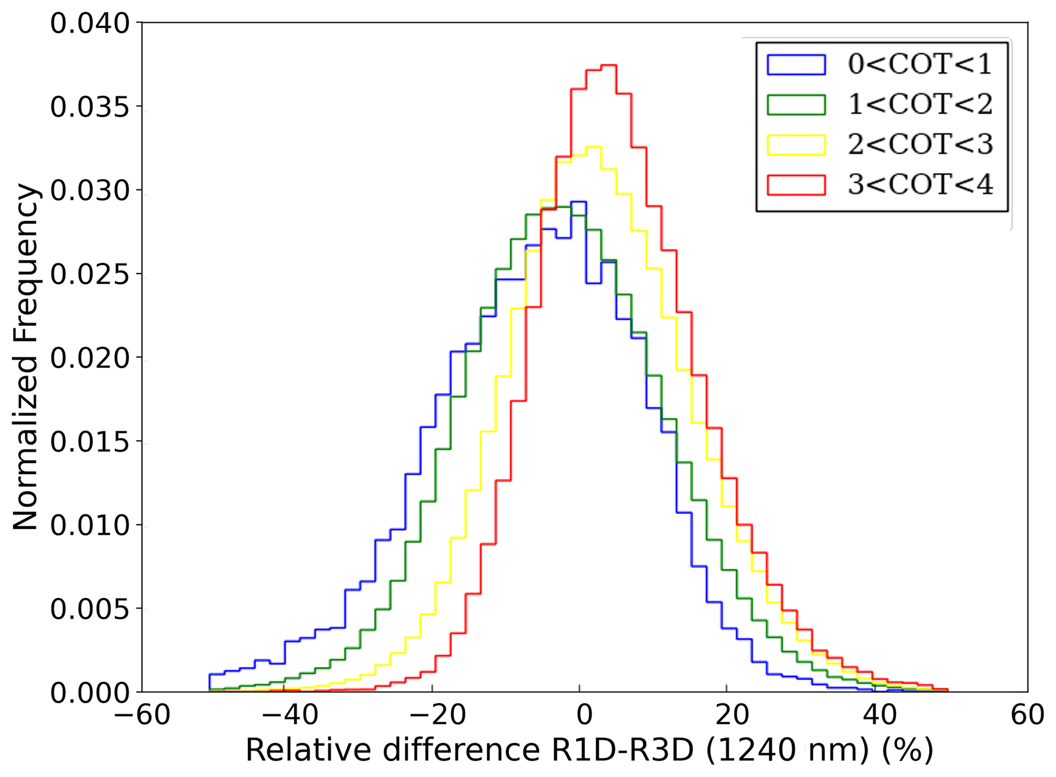
Figure 9Histograms of the relative difference between the reflectances computed in 1D and 3D at 1240 nm for the central image. Each histogram corresponds to a domain of COT.
In Fig. 9, histograms of the relative difference between the radiances computed in 1D (R1D) and the radiances computed in 3D (R3D) at 1240 nm for different bins of optical thickness are plotted. We can see the shift of the histograms from negative values for small optical thickness (R1D < R3D) towards positive differences for larger optical thickness (R1D > R3D) that is explained by the horizontal radiation transport between columns.
Overall, we note that the uncertainties due to the forward model assumption are much more important than the ones due to the fixed parameters. The retrieval is not sensitive to small variations in the fixed parameters. However, while assessing uncertainties due to the vertical profile or radiative transfer assumption, we change the parameters that our forward model is proven to depend on, and thus changes in the integrated profile can lead to relatively large variations in the radiance fields and consequently large uncertainties.
The same strategy applied in Sect. 4 is applied using the bispectral mono-angular method used for the MODIS instrument. For the mono-angular bispectral approach, the measurement vector y for each pixel contains two mono-angular total radiances, one at 1240 nm and the other at 2200 nm. The mono-angular direction corresponds to that of the central image of the multi-angular sequence used to retrieve COT and Reff with the multi-angular measurements.
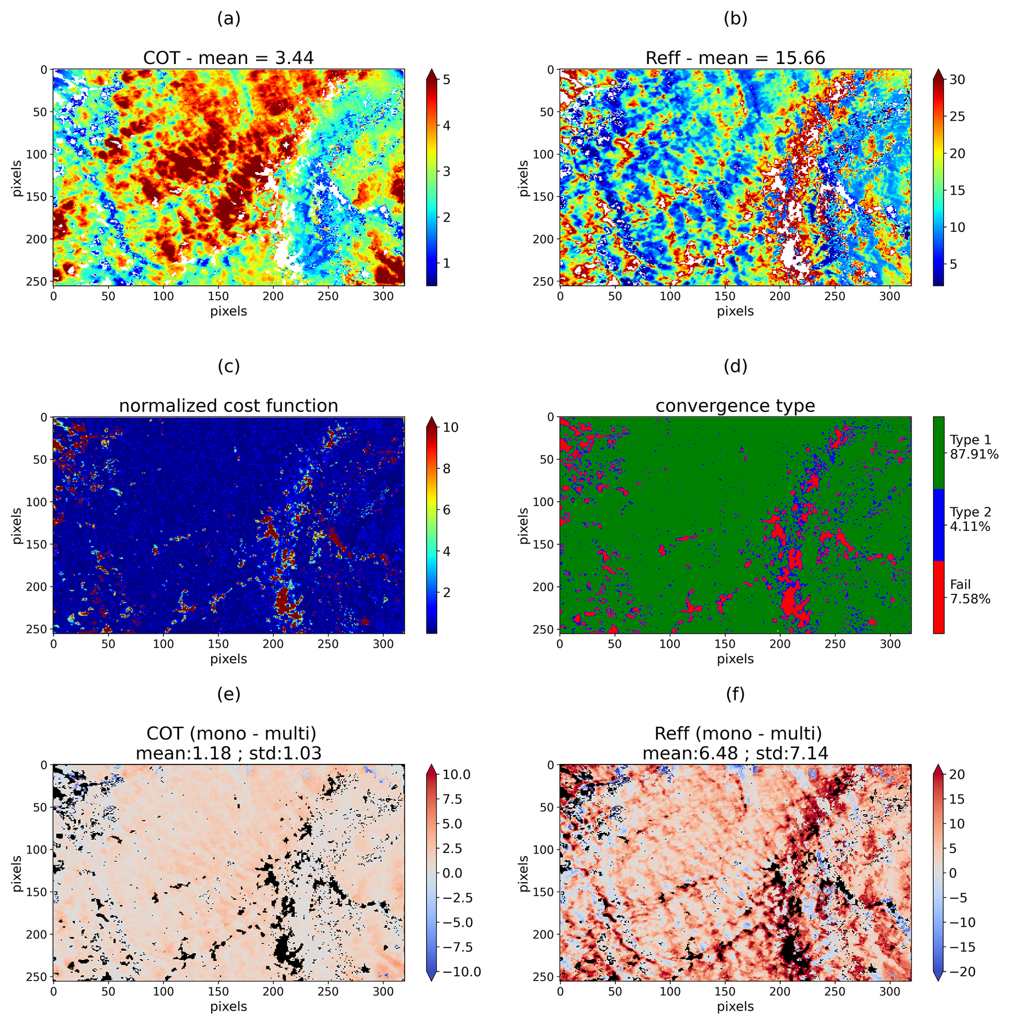
Figure 10COT (a) and Reff (b) retrieved using the mono-angular bispectral method for the CALIOSIRIS liquid cloud case study on 30 June 2014 at 11:02 LT (local time). Pixels associated with failed retrievals are represented by white pixels. (c) Normalized cost function. (d) Convergence type (Eq. 6 for Type 1 and Eq. 7 for Type 2) and failed retrieval. Differences between mono-angular and multi-angular retrieval for retrieved optical thickness (e) and retrieved effective radius (f).
The results are presented in Fig. 10. The retrieved COT over the whole field varies between 1 and 12 with a mean value equal to 3.44. Compared to multi-angular measurements (mean COT of 2.13), the retrieved COT values tend to be higher. The range of retrieved Reff has a mean value of 15.65 µm compared to 8.76 µm for multi-angular retrieval. Mono-angular retrieval is particularly affected by the high value of Reff retrieved around the scattering angles 130–140∘, where the sensitivity of 2200 nm radiances to the water droplet size is known to be small. This area also corresponds to a more important number of failed retrievals. As a matter of fact, Cho et al. (2015) have indeed shown that in liquid marine cloud cases, the phase functions of different Reff converge to the same value for these scattering angle ranges, leading to the failure of water droplet size retrieval from MODIS measurements. This reduced sensitivity also explains the high uncertainty in Reff due to measurement errors around the cloudbow (Fig. 11). The smaller sensitivity to Reff, in this case, is not limited to the cloudbow directions and supernumerary bows but is also visible in some regions of small scattering angles (70–80∘) that can be affected by specular reflection over the ocean.
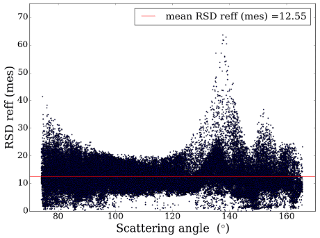
Figure 11Uncertainties in the effective radius originating from the measurement errors, RSD Reff (mes), as a function of the scattering angle for the mono-angular retrieval. The red line represents the mean RSD Reff (mes) = 12.55 %.
Multi-angular retrieval presents the major advantage that no aberrant values of Reff are retrieved near the scattering angles at 140∘ (comparing Fig. 4b to Fig. 10b). The multi-angular measurements contain more information and allow resolving the problem encountered with the mono-angular bispectral method, which is also clear in the reduction of the failed convergences from 7.6 % to 3.3 %. In the overall scene, smaller Reff values are obtained. The smallest effective radius leads to an increase in the backward scattering and therefore in the reflected radiance, which results in a lower retrieved optical thickness.
Except in the case of failed retrievals that occur for values outside the LUT ranges, the relation between radiances and COT–Reff being monotonical, the mono-directional method allows always finding retrieved values: that is, a pair of COT and Reff that matches the measured radiances. However, these values can be more or less far from the real values. A normalized cost function value (Fig. 10c) less than or equal to 1 is thus not necessarily an indication of an accurate retrieval, but only that a fit occurred. On the other hand, multi-angular retrieval increases the constraint on the forward model, which makes it much more challenging to find a solution allowing a fit to the measurements. The retrieved state is then consistent at best with all the measurements associated with different viewing angles.
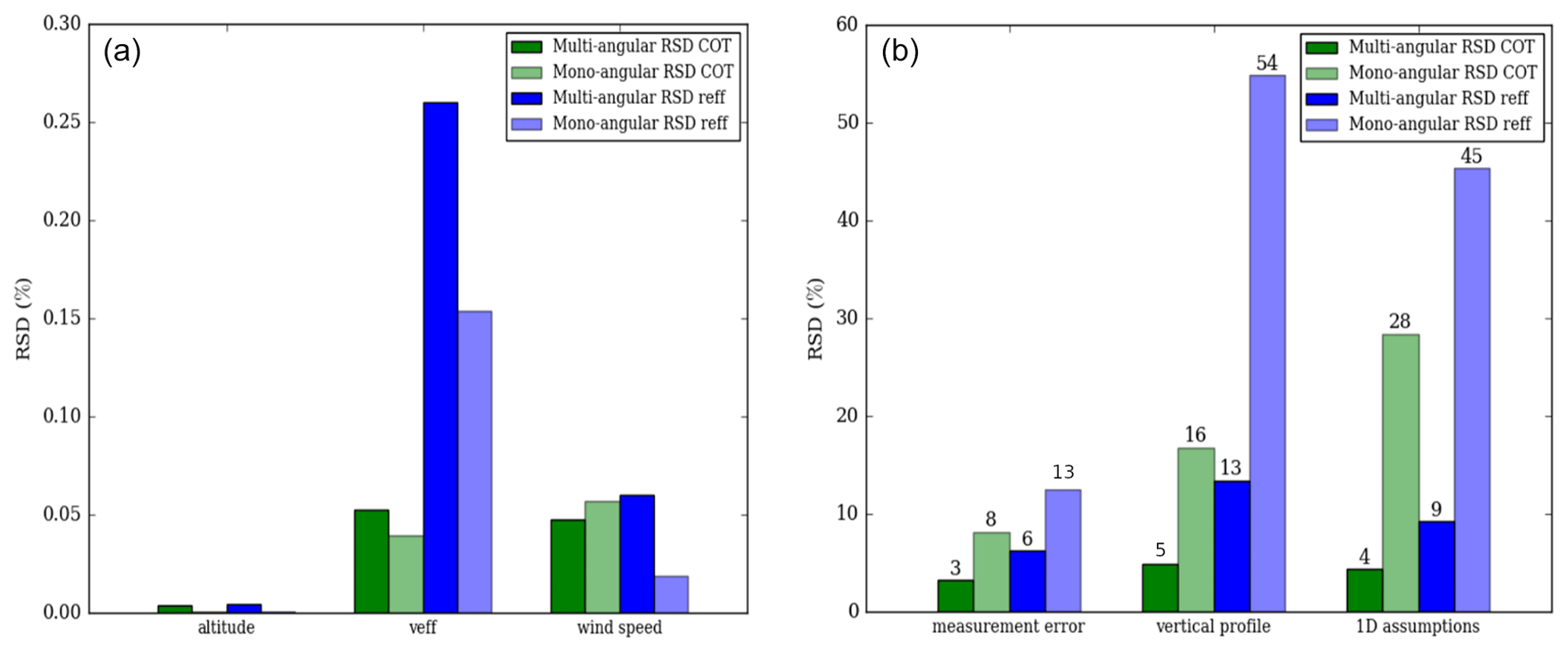
Figure 12Bar chart of the mean uncertainties of the retrieved COT and Reff: green bars correspond to RSD COT and blue bars to RSD Reff. Dark colors correspond to multi-angular retrieval and light colors to mono-angular retrieval. The errors originating from the fixed parameter errors are in (a) and the measurements and forward model errors are in (b).
To compare the uncertainties of the two retrievals, we use the relative standard deviation (RSD) to be consistent with the previous results. In Fig. 12, we present the spatial average of the different types of errors, presented in Sect. 4, for the mono-angular method (light green for COT and light blue for Reff) in comparison with the multi-angular method (dark green for COT and dark blue for Reff). We divide the source of errors into two panels: the left panel (Fig. 12a) groups the lowest values of RSD and the right panel (Fig. 12b) for the highest values of RSD.
Overall, Reff uncertainties are larger than the ones in COT for any type of error. In Fig. 12a, the three fixed model parameters errors related to an incorrect estimation of the fixed parameters of the model are weak compared to the others and remain below 0.3 % for mono-angular retrievals. As explained in Sect. 4, the fixed altitude does not contribute to the uncertainty in the two retrieved parameters. The average uncertainties originating from the fixed value of veff are about 0.05 % for COT and slightly higher (0.15 %) for Reff since veff affects the cloudbows that are also sensitive to Reff. Concerning the surface wind speed, the uncertainties are around an average of 0.05 %.
In Fig. 12b, for mono-angular retrieval, the measurement errors contribute to an uncertainty of about 8 % in the retrieved COT and about 13 % in the retrieved Reff. The uncertainties are reduced by a factor of 2 compared to multi-angular retrieval. The multi-angular approach indeed leads to more information available for each cloudy pixel, and each additional piece of information reduces the uncertainty in the retrieved parameters in the presence of the same 5 % random noise in the measurements.
The following two groups of bars correspond to the errors introduced by the cloud homogeneous assumption used in the forward model. They are the main source of errors. For mono-angular retrieval, the assumption of a vertical homogeneous profile contributes to an uncertainty of about 16 % in COT and 54 % in Reff. These uncertainties are reduced by a factor of 4 in the case of multi-angular retrieval. As discussed previously, the principal effects of 1D assumption errors at the spatial resolution of OSIRIS come from the non-independence of the cloud columns that lead to smoothing the 3D radiative fields and increasing the heterogeneity along the line of sight (Fauchez et al., 2018). They lead to an uncertainty of 28 % in COT and 45 % in Reff when a mono-angular instrument is used.
The multi-angular approach provides additional information for each pixel and constrains the forward model to match all the angular radiances at once. As seen, the OSIRIS multi-angular characteristics have the advantage of decreasing the angular effects around the cloudbow directions by adding the contribution of other geometries and mitigating the sensitivity of the retrieval issued from the assumptions in the forward model. It avoids most of the failed convergences that occurred with the mono-angular bispectral method and retrieved more homogeneous and coherent COT and Reff fields.
In this study, we present a method to retrieve two important microphysical and optical parameters of liquid clouds, COT and Reff, as well as their uncertainties using NIR–SWIR multi-angular airborne measurements. The algorithm is based on the mathematical framework of the optimal estimation method (Rodgers, 2000) and focuses on assessing the different uncertainties of the retrieved properties originating from different sources of errors.
The studied case uses the measurements of the airborne radiometer OSIRIS obtained during the CALIOSIRIS campaign. It consists of a monolayer water cloud located at 5 km altitude over the ocean with tilted solar incidence (θs = 59∘).
In the first step of the retrieval, COT and Reff are retrieved by considering only the measurement errors (without introducing any error linked to the forward model). The uncertainties originating from different sources of error are computed afterward by using the previously retrieved COT and Reff and are decomposed into three different sources related to (a) the instrument measurement errors, (b) an incorrect estimation of the fixed model parameters such as the ocean surface wind, the cloud altitude, and the effective variance of water droplet distribution, and (c) the errors related to the vertically and horizontally homogeneous cloud assumptions. The computations are done using the multi-angular method and for comparison a mono-angular method, which is the usual approach in the operational algorithm.
In the multi-angular retrieval, a 5 % measurement error contributes to around 3 % uncertainty in the retrieved COT and 6 % in the retrieved Reff. It tends to increase with increasing values of COT and Reff to which the sensitivity of radiances starts to decrease. Since they are not characterized, the correlations between the measurement errors issued from different viewing angles are not considered in our retrieval, but they could increase these values. Nevertheless, when considering a mono-angular retrieval, these uncertainties are doubled.
The uncertainties related to the fixed parameters remain low with both mono- and multi-angular retrieval. The largest one is due to the unknown value of the effective variance of the droplet size and is respectively equal to 0.15 % and 0.25 % for the mono- and multi-angular cases. Note that, since the information provided by lidar or polarized measurements was used, the uncertainty for the non-retrieved parameters was chosen to be low. For applications to cases without this available information, errors would be higher. If the method is applied to 3MI for example, the errors related to the cloud-top altitude would be higher as the O2 A-band leads to cloud-top pressure uncertainties between 40 and 80 hPa depending on the cloud types (Desmons et al., 2013). A more complex algorithm could also be used with a measurement vector including O2 A-band radiances and multi-angular polarized radiances to have information on and to add the cloud-top altitude and the effective variance (Huazhe et al., 2019) in the state vector.
This study clearly shows that the largest uncertainty is due to the homogeneous cloud assumption made in our forward model. First, the uncertainties related to the homogeneous vertical profile were quantified using a heterogeneous LWC profile with a triangle shape (known as quasi-adiabatic) composed of two adiabatic profiles. This more realistic profile takes into account the transition zone at the top of the cloud related to turbulent and evaporation processes. The scene-averaged values reach 5 % and 13 % for COT and Reff, respectively, in the multi-angular retrieval of our case study and go up to 16 % and 54 % for COT and Reff, respectively, when using mono-angular measurements. The largest uncertainties are obtained for the largest cloud optical thickness as the radiation samples only the higher layers of the cloud where the information is different between the homogeneous and heterogeneous vertical profiles.
The other sources of uncertainty related to the simplified cloud physical model come from the radiative non-independence of the cloudy columns that dominate at the high spatial resolution of OSIRIS. In the optically thin overcast cloud case studied here, the scene average uncertainties originating from the 3D effects are 4 % for COT and 9 % for Reff when using multi-angular measurements and 28 % for COT and 45 % for Reff when using mono-angular measurements. The non-independence of the cloud columns dominates and tends on one hand to smooth the 3D radiative field compared to radiances computed with the independent pixel approximation and on the other hand to increase the cloud property heterogeneity along the line of sight.
The method was applied to real data, which means that the true cloud parameters are unknown. Consequently, it is not possible to know if real errors in the retrieved parameters are included in the uncertainties given by the method presented here. One factor that can lead to an erroneous assessment is that the estimations of the uncertainties are done around retrieved values that can be biased. A way to check the consistency of the method and the validity of the uncertainty ranges would be to simulate radiances using a large eddy simulation model with a realistic cloud physical description, add noise for the error measurements, and derive the cloud parameters and their uncertainties.
The method presented here can be adapted to the future 3MI. The first step, which consists of including the uncertainties related to the measurement errors, is directly implementable in an operational algorithm. The second step, which consists of computing the uncertainties resulting from the non-retrieved parameters, is more computationally expensive but could also be included. The uncertainties related to the non-retrieved parameters, in addition to the one related to measurement errors, have already been implemented since Collection 5 in the MODIS operational algorithm through the computation of a covariance matrix wherein Jacobians are derived from lookup table and completed for Collection 6 (Platnick et al., 2017). Concerning the forward model errors, the method cannot be implemented as in this work in an operational algorithm because of the prohibitive computation time, but a climatology based on several case studies, depending on the type of clouds, a land or ocean surface flag, for example, could be used in order to obtain a distribution of the errors according to the scene characteristics.
The results obtained in this study show, not surprisingly regarding the numerous studies already published, that the vertical and horizontal homogeneity assumptions are major contributors to the retrieval uncertainties. One way to reduce it would be to define a more complex cloud model that can take into account the vertical and horizontal heterogeneity. This adds more complexity to the forward model as it would imply retrieving more sophisticated cloud parameters (e.g., extinction or effective size profile). It appears, however, possible given the important and complementary information provided by OSIRIS or 3MI measurements. Recent studies proposed retrieving vertical profiles using cloud-side information (Ewald et al., 2018; Saito et al., 2019, Alexandrov et al., 2020) or realizing multi-pixel retrieval to account for the non-independence of the cloudy pixels (Martin et al., 2014; Okamura et al., 2017; Levis et al., 2015), and their implementation could be studied.
Data and codes are available upon request to the authors.
CM developed the inversion algorithms and performed the analysis of the results with the support of CC, FP, and LCL. FA and FP participated in the CALIOSIRIS airborne campaign. FA and JMN made the calibration and OSIRIS data processing from level 0 to level 1. All authors discussed the results and contributed to the final paper.
The contact author has declared that none of the authors has any competing interests.
Publisher's note: Copernicus Publications remains neutral with regard to jurisdictional claims in published maps and institutional affiliations.
The authors thank Guillaume Merlin and Anthony Davis for fruitful discussions concerning the cloud vertical heterogeneous profile. Airborne data were obtained using the aircraft managed by Safire, the French Facility for Airborne Research, an infrastructure of the French National Center for Scientific Research (CNRS), Météo-France, and the French National Center for Space Studies (CNES).
This work has been supported by the Programme National de Télédétection Spatiale (PNTS, https://programmes.insu.cnrs.fr/transverse/pnts/, last access: 15 January 2023) (grant no. PNTS-2017-03) and by the CPER research project CLIMIBIO. The authors received financial support from the French Ministère de l'Enseignement Supérieur et de la Recherche, the Hauts-de-France Region, and European Funds for Regional Economical Development.
This paper was edited by Alexander Kokhanovsky and reviewed by two anonymous referees.
Alexandrov, M. D., Cairns, B., Emde, C., Ackerman, A. S., and van Diedenhoven, B.: Accuracy assessments of cloud droplet size retrievals from polarized reflectance measurements by the research scanning polarimeter, Remote Sens. Environ., 125, 92–111, https://doi.org/10.1016/j.rse.2012.07.012, 2012.
Alexandrov, M. D., Miller, D. J., Rajapakshe, C., Fridlind, A., van Diedenhoven, B., Cairns, B., Ackerman, A. S., and Zhang, Z.: Vertical profiles of droplet size distributions derived from cloud-side observations by the research scanning polarimeter: Tests on simulated data, Atmos. Res., 239, 104924, https://doi.org/10.1016/j.atmosres.2020.104924, 2020.
Auriol, F., Léon, J.-F., Balois, J.-Y., Verwaerde, C., François, P., Riedi, J., Parol, F., Waquet, F., Tanré, D., and Goloub, P.: Multidirectional visible and shortwave infrared polarimeter for atmospheric aerosol and cloud observation: OSIRIS (Observing System Including PolaRisation in the Solar Infrared Spectrum), in: Proceedings of SPIE 7149, Multispectral, Hyperspectral, and Ultraspectral Remote Sensing Technology, Techniques, and Applications II, Noumea, New Caledonia, 17–21 November 2008, https://doi.org/10.1117/12.806421, 2008.
Benner, T. C. and Evans, K. F.: Three-dimensional solar radiative transfer in small tropical cumulus fields derived from high-resolution imagery, J. Geophys. Res.-Atmos., 106, 14975–14984, https://doi.org/10.1029/2001JD900158, 2001.
Bréon, F.-M., and Goloub, P.: Cloud droplet effective radius from spaceborne polarization measurements, Geophys. Res. Lett., 25, 1879–1882, https://doi.org/10.1029/98GL01221, 1998.
Bruneau, D., Pelon, J., Blouzon, F., Spatazza, J., Genau, P., Buchholtz, G., Amarouche, N., Abchiche, A., and Aouji, O.: 355-nm high spectral resolution airborne lidar LNG: system description and first results, Appl. Optics, 54, 8776–8785, https://doi.org/10.1364/AO.54.008776, 2015.
Buriez, J. C., Vanbauce, C., Parol, F., Goloub, P., Herman, M., Bonnel, B., Fouquart, Y., Couvert, P., and Seze, G.: Cloud detection and derivation of cloud properties from POLDER, Int. J. Remote Sens., 18, 2785–2813, https://doi.org/10.1080/014311697217332, 1997.
Cahalan, R. F., Ridgway, W., Wiscombe, W. J., Gollmer, S., and Harshvardhan: Independent Pixel and Monte Carlo Estimates of Stratocumulus Albedo, J. Atmos. Sci., 51, 3776–3790, https://doi.org/10.1175/1520-0469(1994)051<3776:IPAMCE>2.0.CO;2, 1994.
Chang, F.: Estimating the vertical variation of cloud droplet effective radius using multispectral near-infrared satellite measurements, J. Geophys. Res., 107, 4257, https://doi.org/10.1029/2001JD000766, 2002.
Chang, I. and Christopher, S. A.: Identifying Absorbing Aerosols above Clouds from the Spinning Enhanced Visible and Infrared Imager Coupled with NASA A-Train Multiple Sensors, IEEE T. Geosci. Remote, 54, 3163–3173, https://doi.org/10.1109/TGRS.2015.2513015, 2016.
Cho, H., Zhang, Z., Meyer, K., Lebsock, M., Platnick, S., Ackerman, A. S., Di Girolamo, L., C.-Labonnote, L., Cornet, C., Riedi, J., and Holz, R. E.: Frequency and causes of failed MODIS cloud property retrievals for liquid phase clouds over global oceans, J. Geophys. Res.-Atmos., 120, 4132–4154, https://doi.org/10.1002/2015JD023161, 2015.
Cooper, S. J., L'Ecuyer, T. S., and Stephens, G. L.: The impact of explicit cloud boundary information on ice cloud microphysical property retrievals from infrared radiances, J. Geophys. Res.-Atmos., 108, 4107, https://doi.org/10.1029/2002JD002611, 2003.
Cornet, C. and Davies, R.: Use of MISR measurements to study the radiative transfer of an isolated convective cloud: Implications for cloud optical thickness retrieval, J. Geophys. Res.-Atmos., 113, 1–11, https://doi.org/10.1029/2007JD008921, 2008.
Cornet, C., Buriez, J., Riédi, J., Isaka, H., and Guillemet, B.: Case study of inhomogeneous cloud parameter retrieval from MODIS data, Geophys. Res. Lett., 32, L13807, https://doi.org/10.1029/2005GL022791, 2005.
Cornet, C., C-Labonnote, L., and Szczap, F.: Three-dimensional polarized Monte Carlo atmospheric radiative transfer model (3DMCPOL): 3D effects on polarized visible reflectances of a cirrus cloud, J. Quant. Spectrosc. Ra., 111, 174–186, https://doi.org/10.1016/j.jqsrt.2009.06.013, 2010.
Cornet, C., C.-Labonnote, L., Waquet, F., Szczap, F., Deaconu, L., Parol, F., Vanbauce, C., Thieuleux, F., and Riédi, J.: Cloud heterogeneity on cloud and aerosol above cloud properties retrieved from simulated total and polarized reflectances, Atmos. Meas. Tech., 11, 3627–3643, https://doi.org/10.5194/amt-11-3627-2018, 2018.
Cox, C. and Munk, W.: Measurement of the Roughness of the Sea Surface from Photographs of the Sun's Glitter, J. Opt. Soc. Am., 44, 838, https://doi.org/10.1364/JOSA.44.000838, 1954.
Davis, A., Marshak, A., Cahalan, R., and Wiscombe, W.: The Landsat Scale Break in Stratocumulus as a Three-Dimensional Radiative Transfer Effect: Implications for Cloud Remote Sensing, J. Atmos. Sci., 54, 241–260, https://doi.org/10.1175/1520-0469(1997)054<0241:TLSBIS>2.0.CO;2, 1997.
De Haan, J., Bosma, P., and Hovenier, J.: The adding method for multiple scattering calculations of polarized light, Astron. Astrophys., 183, 371–391, 1987.
Deschamps, P.-Y., Breon, F.-M., Leroy, M., Podaire, A., Bricaud, A., Buriez, J.-C., and Seze, G.: The POLDER mission: instrument characteristics and scientific objectives, IEEE T. Geosci. Remote, 32, 598–615, https://doi.org/10.1109/36.297978, 1994.
Desmons, M., Ferlay, N., Parol, F., Mcharek, L., and Vanbauce, C.: Improved information about the vertical location and extent of monolayer clouds from POLDER3 measurements in the oxygen A-band, Atmos. Meas. Tech., 6, 2221–2238, https://doi.org/10.5194/amt-6-2221-2013, 2013.
Elsaesser, G. S. and Kummerow, C. D.: Toward a Fully Parametric Retrieval of the Nonraining Parameters over the Global Oceans, J. Appl. Meteorol. Clim., 47, 1599–1618, https://doi.org/10.1175/2007JAMC1712.1, 2008.
Ewald, F., Zinner, T., Kölling, T., and Mayer, B.: Remote sensing of cloud droplet radius profiles using solar reflectance from cloud sides – Part 1: Retrieval development and characterization, Atmos. Meas. Tech., 12, 1183–1206, https://doi.org/10.5194/amt-12-1183-2019, 2019.
Fauchez, T., Platnick, S., Várnai, T., Meyer, K., Cornet, C., and Szczap, F.: Scale dependence of cirrus heterogeneity effects. Part II: MODIS NIR and SWIR channels, Atmos. Chem. Phys., 18, 12105–12121, https://doi.org/10.5194/acp-18-12105-2018, 2018.
Formenti, P., D’Anna, B., Flamant, C., Mallet, M., Piketh, S. J., Schepanski, K., Waquet, F., Auriol, F., Brogniez, G., Burnet, F., Chaboureau, J., Chauvigné, A., Chazette, P., Denjean, C., Desboeufs, K., Doussin, J., Elguindi, N., Feuerstein, S., Gaetani, M., Giorio, C., Klopper, D., Mallet, M. D., Nabat, P., Monod, A., Solmon, F., Namwoonde, A., Chikwililwa, C., Mushi, R., Welton, E. J., and Holben, B.: The Aerosols, Radiation and Clouds in Southern Africa Field Campaign in Namibia: Overview, Illustrative Observations, and Way Forward, B. Am. Meteorol. Soc., 100, 1277–1298, https://doi.org/10.1175/BAMS-D-17-0278.1, 2019.
Garnier, A., Pelon, J., Dubuisson, P., Faivre, M., Chomette, O., Pascal, N., and Kratz, D. P.: Retrieval of Cloud Properties Using CALIPSO Imaging Infrared Radiometer. Part I: Effective Emissivity and Optical Depth, J. Appl. Meteorol. Clim., 51, 1407–1425, https://doi.org/10.1175/JAMC-D-11-0220.1, 2012.
Giraud, V., Buriez, J. C., Fouquart, Y., Parol, F., and Seze, G.: Large-scale analysis of cirrus clouds from AVHRR data: Assessment of both a microphysical index and the cloud-top temperature, J. Appl. Meteorol., 36, 664–675, https://doi.org/10.1175/1520-0450-36.6.664, 1997.
Hagolle, O., Goloub, P., Deschamps, P.-Y., Cosnefroy, H., Briottet, X., Bailleul, T., Nicolas, J.-M., Parol, F., Lafrance, B., and Herman, M.: Results of POLDER in-flight calibration, IEEE T. Geosci. Remote, 37, 1550–1566, https://doi.org/10.1109/36.763266, 1999.
Hansen, J. E. and Travis, L. D.: Light scattering in planetary atmospheres, Space Sci. Rev., 16, 527–610, https://doi.org/10.1007/BF00168069, 1974.
Hickey, J. R. and Karoli, A. R.: Radiometric Calibrations for the Earth Radiation Budget Experiment, Appl. Opt., 13, 523, https://doi.org/10.1364/AO.13.000523, 1974.
Huazhe, S., Letu, H., Bréon, F.-M., Riedi, J., Ma, R., Wang, Z., Nakajima, T. Y., Wang, Z., and Chen, L.: An improved algorithm of cloud droplet size distribution from POLDER polarized measurements, Remote Sens. Environ., 228, 61–74, https://doi.org/10.1016/j.rse.2019.04.013, 2019.
Inoue, T.: On the Temperature and Effective Emissivity Determination of Semi-Transparent Cirrus Clouds by Bi-Spectral Measurements in the 10 µm Window Region, J. Meteorol. Soc. Jpn. Ser. II, 63, 88–99, https://doi.org/10.2151/jmsj1965.63.1_88, 1985.
IPCC: Climate Change 2021: The Physical Science Basis. Contribution of Working Group I to the Sixth Assessment Report of the Intergovernmental Panel on Climate Change, edited by: Masson-Delmotte, V., Zhai, P., Pirani, A., Connors, S. L., Péan, C., Berger, S., Caud, N., Chen, Y., Goldfarb, L., Gomis, M. I., Huang, M., Leitzell, K., Lonnoy, E., Matthews, J. B. R., Cambridge University Press, Cambridge, United Kingdom and New York, NY, USA, in press, https://doi.org/10.1017/9781009157896, 2021.
Iwabuchi, H., Saito, M., Tokoro, Y., Putri, N. S., and Sekiguchi, M.: Retrieval of radiative and microphysical properties of clouds from multispectral infrared measurements, Progress in Earth and Planetary Science, 3, 32, https://doi.org/10.1186/s40645-016-0108-3, 2016.
Kato, S. and Marshak, A.: Solar zenith and viewing geometry-dependent errors in satellite retrieved cloud optical thickness: Marine stratocumulus case, J. Geophys. Res.-Atmos., 114, 1–13, https://doi.org/10.1029/2008JD010579, 2009.
Kaufman, Y. J., Tanré, D., and Boucher, O.: A satellite view of aerosols in the climate system, Nature, 419, 215–223, https://doi.org/10.1038/nature01091, 2002.
Kokhanovsky, A. and Rozanov, V. V.: Droplet vertical sizing in warm clouds using passive optical measurements from a satellite, Atmos. Meas. Tech., 5, 517–528, https://doi.org/10.5194/amt-5-517-2012, 2012.
Kollias, P., Szyrmer, W., Rémillard, J., and Luke, E.: Cloud radar Doppler spectra in drizzling stratiform clouds: 2. Observations and microphysical modeling of drizzle evolution, J. Geophys. Res.-Atmos., 116, D13203, https://doi.org/10.1029/2010JD015238, 2011.
Levenberg, K.: A method for the solution of certain non-linear problems in least squares, Q. Appl. Math., 2, 164–168, https://doi.org/10.1090/qam/10666, 1944.
Levis, A., Schechner, Y. Y., Aides, A., and Davis, A. B.: Airborne Three-Dimensional Cloud Tomography, IEEE International Conference on Computer Vision (ICCV), 3379–3387, https://doi.org/10.1109/ICCV.2015.386, 2015.
Lohmann, U. and Feichter, J.: Global indirect aerosol effects: a review, Atmos. Chem. Phys., 5, 715–737, https://doi.org/10.5194/acp-5-715-2005, 2005.
Mallet, M., Dulac, F., Formenti, P., Nabat, P., Sciare, J., Roberts, G., Pelon, J., Ancellet, G., Tanré, D., Parol, F., Denjean, C., Brogniez, G., di Sarra, A., Alados-Arboledas, L., Arndt, J., Auriol, F., Blarel, L., Bourrianne, T., Chazette, P., Chevaillier, S., Claeys, M., D'Anna, B., Derimian, Y., Desboeufs, K., Di Iorio, T., Doussin, J.-F., Durand, P., Féron, A., Freney, E., Gaimoz, C., Goloub, P., Gómez-Amo, J. L., Granados-Muñoz, M. J., Grand, N., Hamonou, E., Jankowiak, I., Jeannot, M., Léon, J.-F., Maillé, M., Mailler, S., Meloni, D., Menut, L., Momboisse, G., Nicolas, J., Podvin, T., Pont, V., Rea, G., Renard, J.-B., Roblou, L., Schepanski, K., Schwarzenboeck, A., Sellegri, K., Sicard, M., Solmon, F., Somot, S., Torres, B., Totems, J., Triquet, S., Verdier, N., Verwaerde, C., Waquet, F., Wenger, J., and Zapf, P.: Overview of the Chemistry-Aerosol Mediterranean Experiment/Aerosol Direct Radiative Forcing on the Mediterranean Climate (ChArMEx/ADRIMED) summer 2013 campaign, Atmos. Chem. Phys., 16, 455–504, https://doi.org/10.5194/acp-16-455-2016, 2016.
Marbach T., Riedi J., Lacan A., and Schlüssel P. : The 3MI mission: multi-viewing-channel-polarisation imager of the EUMETSAT polar system: second generation (EPS-SG) dedicated to aerosol and cloud monitoring, Proc. SPIE 9613, Polarization Science and Remote Sensing VII, https://doi.org/10.1117/12.2186978, 2015.
Marquardt, D. W.: An Algorithm for Least-Squares Estimation of Nonlinear Parameters, J. Soc. Ind. Appl. Math., 11, 431–441, https://doi.org/10.1137/0111030, 1963.
Marshak, A., Davis, A., Wiscombe, W., and Titov, G.: The verisimilitude of the independent pixel approximation used in cloud remote sensing, Remote Sens. Environ., 52, 71–78, https://doi.org/10.1016/0034-4257(95)00016-T, 1995.
Marshak, A., Platnick, S., Várnai, T., Wen, G., and Cahalan, R. F.: Impact of three-dimensional radiative effects on satellite retrievals of cloud droplet sizes, J. Geophys. Res., 111, D09207, https://doi.org/10.1029/2005JD006686, 2006.
Martin, W., Cairns, B., and Bal, G.: Adjoint methods for adjusting three-dimensional atmosphere and surface properties to fit multi-angle/multi-pixel polarimetric measurements, J. Quant. Spectrosc. Ra., 144, 68–85, https://doi.org/10.1016/j.jqsrt.2014.03.030, 2014.
McClatchey, R. A., Fenn, R. W., Selby, J. E. A., Volz, F. E., and Garing, J. S.: Optical Properties of the Atmosphere, 3rd Edn., AIR FORCE CAMBRIDGE RESEARCH LABS HANSCOM AFB MA., Defense Technical Information Center, AFCRL-TR-720497, AD715270, 1972.
Merlin, G.: Préparation à l'exploitation des observationsmulti-spectrales, multi-angulaires et polarisées de l'instrument 3MI pour les atmosphères nuageuses, PhD thesis, University of Lille, France, 2016LIL10184, 212 pp., 2016.
Miles, N. L., Verlinde, J., and Clothiaux, E. E.: Cloud Droplet Size Distributions in Low-Level Stratiform Clouds, J. Atmos. Sci.. 57. 295–311, https://doi.org/10.1175/1520-0469(2000)057<0295:CDSDIL>2.0.CO;2, 2000.
Miller, D. J., Zhang, Z., Ackerman, A. S., Platnick, S., and Baum, B. A.: The impact of cloud vertical profile on liquid water path retrieval based on the bispectral method: A theoretical study based on large-eddy simulations of shallow marine boundary layer clouds, J. Geophys. Res.-Atmos., 121, 4122–4141, https://doi.org/10.1002/2015JD024322, 2016.
Nakajima, T. and King, M. D.: Determination of the Optical Thickness and Effective Particle Radius of Clouds from Reflected Solar Radiation Measurements. Part I: Theory, J. Atmos. Sci., 47, 1878–1893, https://doi.org/10.1175/1520-0469(1990)047<1878:DOTOTA>2.0.CO;2, 1990.
Nakajima, T. Y., Suzuki, K., and Stephens, G. L.: Droplet Growth in Warm Water Clouds Observed by the A-Train. Part II: A Multisensor View, J. Atmos. Sci., 67, 1897–1907, https://doi.org/10.1175/2010JAS3276.1, 2010.
Okamura, R., Iwabuchi, H., and Schmidt, K. S.: Feasibility study of multi-pixel retrieval of optical thickness and droplet effective radius of inhomogeneous clouds using deep learning, Atmos. Meas. Tech., 10, 4747–4759, https://doi.org/10.5194/amt-10-4747-2017, 2017.
Oreopoulos, L. and Davies, R.: Plane Parallel Albedo Biases from Satellite Observations. Part I: Dependence on Resolution and Other Factors, J. Climate, 11, 919–932, https://doi.org/10.1175/1520-0442(1998)011<0919:PPABFS>2.0.CO;2, 1998.
Oreopoulos, L. and Platnick, S.: Radiative susceptibility of cloudy atmospheres to droplet number perturbations: 2. Global analysis from MODIS, J. Geophys. Res., 113, D14S21, https://doi.org/10.1029/2007JD009655, 2008.
Parol, F., Buriez, J. C., Brogniez, G., and Fouquart, Y.: Information Content of AVHRR Channels 4 and 5 with Respect to the Effective Radius of Cirrus Cloud Particles, J. Appl. Meteorol., 30, 973–984, https://doi.org/10.1175/1520-0450-30.7.973, 1991.
Platnick, S.: Vertical photon transport in cloud remote sensing problems, J. Geophys. Res.-Atmos., 105, 22919–22935, https://doi.org/10.1029/2000JD900333, 2000.
Platnick, S., King, M. D., Ackerman, S. A., Menzel, W. P., Baum, B. A., Riedi, J. C., and Frey, R. A.: The MODIS cloud products: algorithms and examples from terra, IEEE T. Geosci. Remote, 41, 459–473, https://doi.org/10.1109/TGRS.2002.808301, 2003.
Platnick, S., Meyer, K. G., D., K. M., Wind, G., Amarasinghe, N., Marchant, B., Arnold, G. T., Zhang, Z., Hubanks, P. A., Holz, R. E., Yang, P., Ridgway, W. L., and Riedi, J.: The MODIS Cloud Optical and Microphysical Products: Collection 6 Updates and Examples From Terra and Aqua, IEEE T. Geosci. Remote, 55, 502–525, https://doi.org/10.1109/TGRS.2016.2610522, 2017.
Poulsen, C. A., Siddans, R., Thomas, G. E., Sayer, A. M., Grainger, R. G., Campmany, E., Dean, S. M., Arnold, C., and Watts, P. D.: Cloud retrievals from satellite data using optimal estimation: evaluation and application to ATSR, Atmos. Meas. Tech., 5, 1889–1910, https://doi.org/10.5194/amt-5-1889-2012, 2012.
Rivoire, L., Birner, T., Knaff, J. A., and Tourville, N.: Quantifying the Radiative Impact of Clouds on Tropopause Layer Cooling in Tropical Cyclones, J. Climate, 33, 6361–6376, https://doi.org/10.1175/JCLI-D-19-0813.1, 2020.
Rodgers, C. D.: Retrieval of atmospheric temperature and composition from remote measurements of thermal radiation, Rev. Geophys., 14, 609, https://doi.org/10.1029/RG014i004p00609, 1976.
Rodgers, C. D.: Inverse methods for atmospheric sounding: Theory and Practice/Series on Atmospheric, Oceanic and Planetary Physics, in: Inverse Methods for Atmospheric Sounding, Vol. 2, World Scientific, Publishing Co. Pte. Ltd., Farrer Road, Singapore 912805 https://doi.org/10.1142/9789812813718_0001, 2000.
Saito, M., Yang, P., Hu, Y., Liu, X., Loeb, N., Smith Jr, W. L., and Minnis, P.: An efficient method for microphysical property retrievals in vertically inhomogeneous marine water clouds using MODIS-CloudSat measurements, J. Geophys. Res.-Atmos., 124, 2174–2193, https://doi.org/10.1029/2018JD029659, 2019.
Seethala, C. and Horváth, Á.: Global assessment of AMSR-E and MODIS cloud liquid water path retrievals in warm oceanic clouds, J. Geophys. Res., 115, D13202, https://doi.org/10.1029/2009JD012662, 2010.
Sourdeval, O., C.-Labonnote, L. C., Brogniez, G., Jourdan, O., Pelon, J., and Garnier, A.: A variational approach for retrieving ice cloud properties from infrared measurements: application in the context of two IIR validation campaigns, Atmos. Chem. Phys., 13, 8229–8244, https://doi.org/10.5194/acp-13-8229-2013, 2013.
Sourdeval, O., C.-Labonnote, L., Baran, A. J., and Brogniez, G.: A methodology for simultaneous retrieval of ice and liquid water cloud properties. Part I: Information content and case study, Q. J. Roy. Meteor. Soc., 141, 870–882, https://doi.org/10.1002/qj.2405, 2015.
Szczap, F., Isaka, H., Saute, M., Guillemet, B., and Ioltukhovski, A.: Effective radiative properties of bounded cascade absorbing clouds: Definition of an effective single-scattering albedo, J. Geophys. Res.-Atmos., 105, 20635–20648, https://doi.org/10.1029/2000JD900145, 2000.
Takahashi, H., Lebsock, M., Suzuki, K., Stephens, G., and Wang, M.: An investigation of microphysics and subgrid-scale variability in warm-rain clouds using the A-Train observations and a multiscale modeling framework, J. Geophys. Res.-Atmos., 122, 7493–7504, https://doi.org/10.1002/2016JD026404, 2017.
Twomey, S.: Aerosols, clouds and radiation, Atmos. Environ. A-Gen., 25, 2435–2442, https://doi.org/10.1016/0960-1686(91)90159-5, 1991.
Van de Hulst, H. C.: A new look at multiple scattering, Tech. Rep., Goddard Institute for Space Studies, NASA TM-I03044, NASA Institute for Space Studies, Goddard Space Flight Center, New York, 1963.
Várnai, T.: Influence of three-dimensional radiative effects on the spatial distribution of shortwave cloud reflection, J. Atmos. Sci., 57, 216–229, https://doi.org/10.1175/1520-0469(2000)057<0216:IOTDRE>2.0.CO;2, 2000.
Várnai, T. and Davies, R.: Effects of Cloud Heterogeneities on Shortwave Radiation: Comparison of Cloud-Top Variability and Internal Heterogeneity, J. Atmos. Sci., 56, 4206–4224, https://doi.org/10.1175/1520-0469(1999)056<4206:EOCHOS>2.0.CO;2, 1999.
Várnai, T. and Marshak, A.: A method for analyzing how various parts of clouds influence each other's brightness, J. Geophys. Res., 108, 4706, https://doi.org/10.1029/2003JD003561, 2003.
Várnai, T. and Marshak, A.: View angle dependence of cloud optical thicknesses retrieved by Moderate Resolution Imaging Spectroradiometer (MODIS), J. Geophys. Res.-Atmos., 112, 1–12, https://doi.org/10.1029/2005JD006912, 2007.
Várnai, T. and Marshak, A.: MODIS observations of enhanced clear sky reflectance near clouds, Geophys. Res. Lett., 36, L06807, https://doi.org/10.1029/2008GL037089, 2009.
Walther, A. and Heidinger, A. K.: Implementation of the Daytime Cloud Optical and Microphysical Properties Algorithm (DCOMP) in PATMOS-x, J. Appl. Meteorol. Clim., 51, 1371–1390, https://doi.org/10.1175/JAMC-D-11-0108.1, 2012.
Wang, C., Platnick, S., Zhang, Z., Meyer, K., and Yang, P.: Retrieval of ice cloud properties using an optimal estimation algorithm and MODIS infrared observations: 1. Forward model, error analysis, and information content, J. Geophys. Res.-Atmos., 121, 5809–5826, https://doi.org/10.1002/2015JD024526, 2016.
Wood, R.: Drizzle in Stratiform Boundary Layer Clouds. Part II: Microphysical Aspects, J. Atmos. Sci., 62, 3034–3050, https://doi.org/10.1175/JAS3530.1, 2005.
Yang, Q., Fu, Q., and Hu, Y.: Radiative impacts of clouds in the tropical tropopause layer, J. Geophys. Res.-Atmos., 115, 1–21, https://doi.org/10.1029/2009JD012393, 2010.
Zhang, Y., Xie, S., Lin, W., Klein, S. A., Zelinka, M., Ma, P., Rasch, P. J., Qian, Y., Tang, Q., and Ma, H.: Evaluation of Clouds in Version 1 of the E3SM Atmosphere Model With Satellite Simulators, J. Adv. Model. Earth Sy., 11, 1253–1268, https://doi.org/10.1029/2018MS001562, 2019.
Zhang, Z. and Platnick, S.: An assessment of differences between cloud effective particle radius retrievals for marine water clouds from three MODIS spectral bands, J. Geophys. Res., 116, D20215, https://doi.org/10.1029/2011JD016216, 2011.
Zhang, Z., Ackerman, A. S., Feingold, G., Platnick, S., Pincus, R., and Xue, H.: Effects of cloud horizontal inhomogeneity and drizzle on remote sensing of cloud droplet effective radius: Case studies based on large-eddy simulations, J. Geophys. Res.-Atmos., 117, D19208, https://doi.org/10.1029/2012JD017655, 2012.
Zinner, T. and Mayer, B.: Remote sensing of stratocumulus clouds: Uncertainties and biases due to inhomogeneity, J. Geophys. Res., 111, D14209, https://doi.org/10.1029/2005JD006955, 2006.
- Abstract
- Introduction
- Instrumentation and airborne campaign
- Retrieval methodology
- Retrieval and uncertainty estimation for a liquid cloud case study measured by OSIRIS
- Advantages of using multi-angular versus mono-angular information
- Conclusions
- Code and data availability
- Author contributions
- Competing interests
- Disclaimer
- Acknowledgements
- Financial support
- Review statement
- References