the Creative Commons Attribution 4.0 License.
the Creative Commons Attribution 4.0 License.
 | 04 Jul 2023
Efficient collocation of global navigation satellite system radio occultation soundings with passive nadir microwave soundings
Alex Meredith
Stephen Leroy
Lucy Halperin
Kerri Cahoy
Radio occultation (RO) using the global navigation satellite system (GNSS) can be used to infer atmospheric profiles of microwave refractivity in the Earth's atmosphere. GNSS RO data are now assimilated into numerical weather prediction models and used for climate monitoring. New remote sensing applications are being considered that fuse GNSS RO soundings and passive nadir-scanned radiance soundings. Collocating RO soundings and nadir-scanned radiance soundings, however, is computationally expensive, especially as new commercial GNSS RO constellations greatly increase the number of global daily RO soundings. This paper develops a new and efficient technique, called the “rotation–collocation method”, for collocating RO and nadir-scanned radiance soundings in which all soundings are rotated into the time-dependent reference frame in which the nadir sounder's scan pattern is stationary. Collocations with RO soundings are then found when the track of an RO sounding crosses the line corresponding to the nadir sounder's scan pattern. When applied to finding collocations between RO soundings from COSMIC-2, Metop-B-GRAS, and Metop-C-GRAS and the passive microwave (MW) soundings of the Advanced Technology Microwave Sounder (ATMS) on NOAA-20 and Suomi-NPP and the Advanced Microwave Sounding Unit (AMSU-A) on Metop-B and Metop-C for the month of January 2021, the rotation–collocation method proves to be 99.0 % accurate and is hundreds to thousands of times faster than traditional approaches to finding collocations.
- Article
(5281 KB) - Full-text XML
- BibTeX
- EndNote


Measurements made using radio occultation (RO) of the Earth's atmosphere from the transmitters of the global navigation satellite system (GNSS) are now routine and important contributors to numerical weather prediction and atmospheric reanalysis (Cardinali and Healy, 2014; Banos et al., 2019, and references therein). GNSS RO data fill in large holes in global coverage left by the international network of radiosondes, anchor atmospheric analyses by virtue of their near-absolute accuracy (Gelaro et al., 2017; Hersbach et al., 2020), and provide cloud-free information on atmospheric water vapor in the middle to lower troposphere (Kursinski and Gebhardt, 2014; Mascio et al., 2021). GNSS RO measurements are typically inverted to yield profiles of the index of refraction, a quantity with contributions from atmospheric density, temperature, and water vapor (Kursinski et al., 2000).
Collocations of GNSS RO atmospheric soundings with the soundings of cross-track scanners in low Earth orbit are useful for several reasons. First, the contributions of water vapor and nitrogen or oxygen to the index of refraction cannot be separated based on RO measurement alone; separating their contributions instead requires the assistance of outside constraints. The commonly used outside constraint is the forecast of a numerical weather prediction system (e.g., Healy and Eyre, 2000), but specialized algorithms have been proposed that implement constraints based on collocated remote soundings by different techniques. One such algorithm considers column water vapor as inferred from microwave radiometers (Xie, 2006; Wang et al., 2017). Second, RO data have been used as a benchmark for investigating the accuracy of other remote sensing instruments by virtue of the near-absolute accuracy of the measurements. RO soundings have been compared to collocated microwave soundings in order to validate the microwave soundings (Schrøder et al., 2003; Ho et al., 2007; Iacovazzi et al., 2020) because microwave radiance standards are far less accurate than the timing standards that underpin the GNSS signals used. GNSS RO validation reduces concerns about the use of satellite microwave data for climate trend studies. Intercomparison of RO and spectral thermal infrared sounders for the sake of validating the calibration of the infrared sounders has also been investigated (Feltz et al., 2017; Yunck et al., 2009). These studies find that collocation between GNSS RO soundings and soundings of passive nadir cross-track scanners is necessary.
The computation of collocation between RO and passive nadir scanners is computationally expensive. Collocation is defined by tolerance windows in the spatial and temporal separation between a pair of RO and passive nadir soundings. The most direct approach to collocation is to consider a large batch of RO soundings and a large batch of passive nadir-scanning data in time periods ΔT significantly longer than the temporal separation window Δt and calculating the temporal and spatial separations between every potential pair of RO and nadir scanner soundings to find pairs that meet the collocation criteria defined by the tolerance windows. Because of the large numbers of passive nadir soundings involved, the computation of collocations is extremely expensive. The expense can be reduced by decreasing the time window on passive nadir scanner soundings to be considered to ΔT=2Δt, but no further optimization is possible. We refer to collocation approaches similar to this as “brute-force” methods. Publicly available tools for collocating satellite data generally use brute-force approaches that are not specific to the geometry of collocating GNSS RO and nadir scanner soundings and instead use parallelization and cloud computing to speed up the finding of collocations (Chung et al., 2022; Smith et al., 2022; Wang et al., 2022).
Another method of collocation is motivated by the density and pattern of passive nadir soundings: they are so dense that they leave no gaps in their coverage during nominal operations, and their coverage pattern can be predicted precisely using an orbit propagator. If the reference frame for a collocation is one in which the scan pattern is just a stationary line of soundings, then a collocation is found when the location of an RO sounding in the scan-pattern reference frame crosses the nadir scanner's scan line. The advantage of such an algorithm is that the actual geolocations and times of the passive nadir soundings need not be considered at all; only the geolocations and times of the RO soundings need to be taken into account. Consequently, the determination of collocations should be greatly accelerated over a brute-force method. The algorithm for collocation involving rotation into the reference frame of the nadir scan pattern we refer to as the “rotation–collocation” method.
The rotation–collocation method implemented in this paper identifies RO soundings that cross the nadir scanner's scan line and predicts the approximate time and location of the closest nadir scanner footprint to these RO soundings, but it does not extract the real nadir scanner footprints collocated with these RO soundings. In order to fairly compare the rotation–collocation method to brute-force methods, the brute-force methods implemented in this paper also do not extract the nadir scanner footprints associated with collocated RO soundings and instead leverage early termination once a collocation is found for faster collocation finding.
The rotation–collocation method promises a great increase in efficiency over any brute-force collocation method, but two complications must be addressed. Each is associated with a key assumption of the rotation–collocation method, and the errors that result must be quantified. The first assumption is that the scan of the passive nadir scanner is defined precisely as a line in its own reference frame. In actuality, rather than a simple line, the scan pattern is a co-linear set of footprints of finite, non-zero sizes and distorted elliptical shapes, with greater distortion at the ends of the scan. The second assumption is that a simple orbit propagator and a range of scan angles of the passive nadir scanner is sufficient to determine the coverage of the scan footprints. These assumptions can be validated and the associated errors quantified by direct comparison of a set of collocations determined by the rotation–collocation method to a set of collocations determined by a brute-force method, with the latter serving as a truth standard. Rates of false positives and false negatives can be estimated. Once these complications are addressed, then all that remains is to compute how great an acceleration in computation is gained by the rotation–collocation method over a standard brute-force method.
This paper is organized as follows. Section 2 contains a description of the brute-force method and a theoretical exposition of the rotation–collocation method. Both will be applied to candidate data sets in order to validate the rotation–collocation method and to determine the acceleration gained by the rotation–collocation method. Section 3 describes the data sets that will be used in the study and defines the experimental setup. Section 4 contains an analysis of the experiments, including a quantification of the daily numbers of collocations of RO soundings with passive nadir microwave soundings. Section 5 presents the final conclusions.
This section describes the details of the brute-force and rotation–collocation algorithms. Collocations are defined as RO soundings that are separated from a passive nadir sounding by at most Δt in time and Δd in distance. We consider the time corresponding to each RO sounding to be the start time of the RO measurement and consider the position corresponding to each RO sounding to be the ray perigee (tangent) point projected onto Earth's surface. First, the details of two approaches to the brute-force algorithm are presented. Following this, two approaches to the rotation–collocation algorithm are presented.
2.1 The brute-force algorithm
The brute-force algorithm uses two checks: a spatial check and a time check. Because the brute-force algorithm makes no approximation, the brute-force method is a truth metric against which the accuracy of our rotation–collocation methods can be evaluated. This subsection describes two implementations of the brute-force algorithm: the first implementation considers all soundings of the nadir scanner over the course of a day when searching for collocations with RO soundings, and the second implementation improves efficiency by sorting the nadir scanner soundings in time and windowing the soundings to within Δt in time of the RO sounding before searching for spatial collocations.
2.1.1 Brute-force method no. 1: all nadir scan soundings
The first brute-force approach compares every RO sounding to every nadir scanner sounding over a 1 d period, performing a spatial check and a time check for every RO–nadir scanner sounding pair. A generic RO sounding has latitude θRO, longitude λRO, and sounding time tRO and a generic nadir scanner sounding has latitude θNS, longitude λNS, and sounding time tNS. The spatial and temporal checks for collocation are as follows:
in which RE is Earth's radius at the Equator and longitudes and latitudes have units of radians. Note that Eq. (1a) assumes small separations, δd≪RE. The temporal check is performed first, which permits a minor speed optimization using early termination: the logging practices of typical nadir scanner instruments generally associate a single time to a fixed number of footprints, thereby permitting a brute-force method to greatly reduce the number of time checks.
2.1.2 Brute-force method no. 2: search–sort
This approach is similar to that of the brute-force method discussed in Sect. 2.1.1 but with narrowed windowing in time. The spatial check remains the same as the one given in Eq. (1a); however, this approach avoids a time check by time-sorting the nadir scanner data. For each RO sounding, we search for the nadir scanner data indices corresponding to the window . Then, we poll the nadir scanner data falling in this time window – which are guaranteed to pass the time check – and perform only the spatial check when searching for collocations.
With n as the total number of nadir scanner soundings and r as the total number of RO soundings, brute-force method no. 1 has a time complexity of O(rn) for the time check. Sorting the nadir scanner data has a time complexity of O(nlog n), where n is the total number of nadir scanner soundings, and searching the nadir scanner data has a time complexity of O(log n), so brute-force method no. 2 has a time complexity of O(rlog n)+O(nlog n) for the time check, as this method performs one initial sort of the nadir scanner data and then one search of the nadir scanner data for each RO sounding.
In most cases, this method is faster than brute-force method no. 1, but when the number of nadir scanner soundings is very large (e.g., log n>r, with n the number of nadir scanner soundings and r the number of RO soundings), the time required to sort the nadir scanner soundings can become long enough that brute-force method no. 2 takes longer than brute-force method no. 1. Furthermore, both brute-force methods avoid performing spatial checks for nadir scanner soundings outside of the time window, so the number of spatial checks performed by both methods is the same. The spatial check is much slower than the time check, so as the time window grows and the number of spatial checks required grows, the time taken by brute-force method no. 2 approaches the time taken by brute-force method no. 1.
2.2 The rotation–collocation algorithm
The rotation–collocation method has two steps: (i) rotating the RO soundings into the nadir-scanning satellite's time-varying frame to find the apparent path of the RO sounding in the reference frame and (ii) determining whether the apparent path of the RO sounding intersects the nadir scanner's pattern. The two patterns can only intersect if both the spatial and the temporal checks are satisfied.
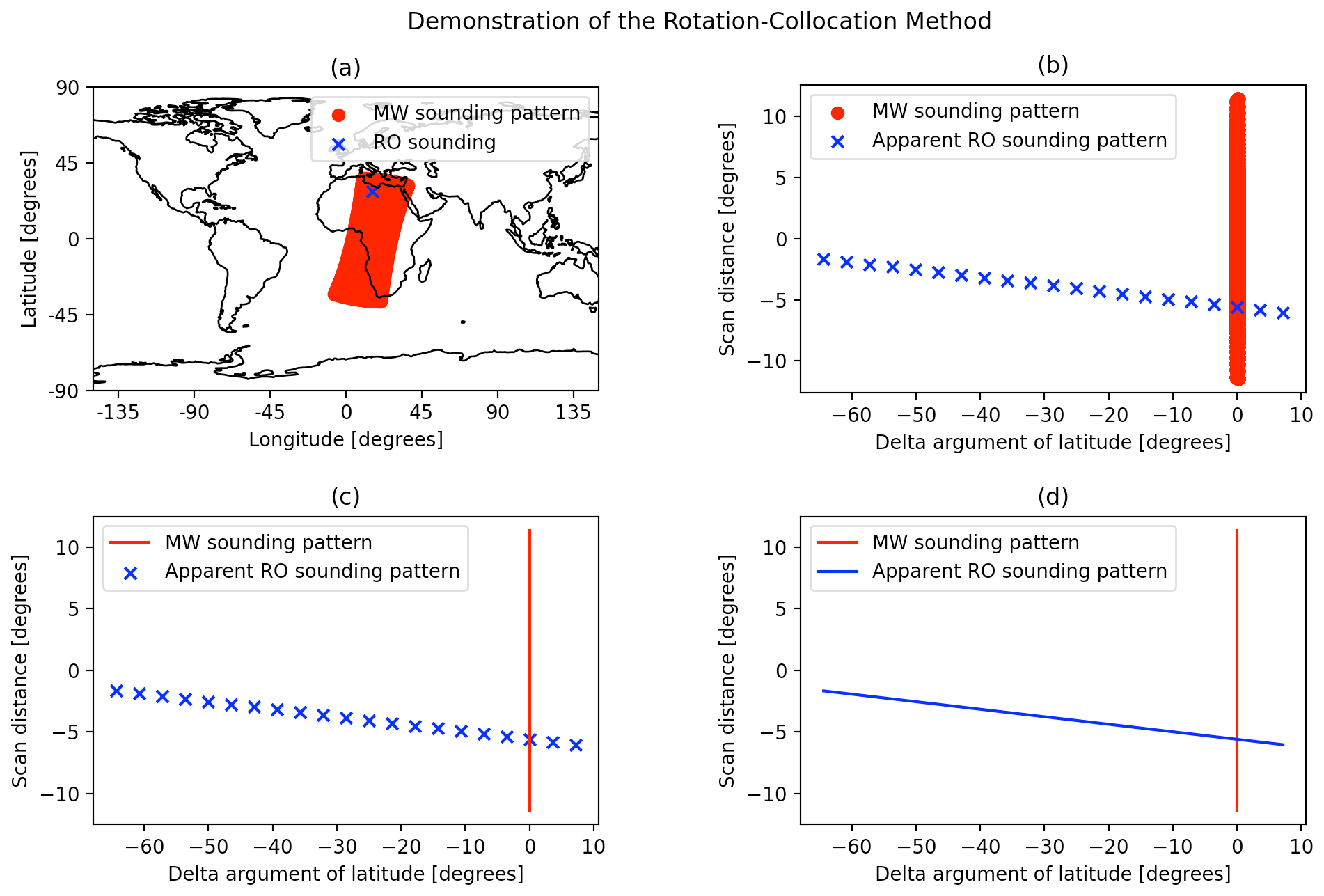
Figure 1(a) A radio occultation from COSMIC-2 E1 plotted against contemporaneous microwave (MW) soundings from NOAA-20 ATMS. (b) The discretized apparent position of the same occultation rotated into the MW frame, plotted against the MW sounding pattern. (c) The discretized apparent position of the RO sounding plotted against the linearized MW sounding pattern. (d) The interpolated apparent position of the RO sounding plotted against the linearized MW sounding pattern.
Figure 1 illustrates the transformations undertaken by the rotation–collocation method. Figure 1a shows an RO sounding from COSMIC-2 E1 occurring at 00:23:52 UTC on 2 January 2021 and the pattern of NOAA-20 Advanced Technology Microwave Sounder (ATMS) soundings occurring within Δt = 600 s of the RO sounding from 00:13:52 to 00:33:52 UTC. Figure 1b shows the COSMIC-2 RO sounding and the ATMS soundings rotated into the time-varying frame of NOAA-20. All of the ATMS soundings collapse to a near-perfect single line that extends upward and downward by an amount related to the range of the nadir scanner's scan angles. Also notice that the single RO sounding is represented as a series of points corresponding to its apparent location in the rotated frame at varying times ti with the time window . In this work, we refer to these apparent locations of a single RO sounding in the time-varying rotated frame as “sub-occultations”, as shown in Fig. 1b and c. The apparent path of the sub-occultations crosses the line of the ATMS scan pattern, indicating the existence of a collocation.
Figure 1c demonstrates the first approximation associated with the rotation–collocation algorithm, which is that a nadir scanner sounding pattern can be approximated by a perfect line at δu=0 with u the argument of latitude or along-track coordinate of the nadir scanner found using an orbit propagator. This approximation rests on three major assumptions: first, that the footprints of the nadir scanner, which are distorted ellipses, can be treated as single points; second, that the orbit propagator used in the rotation is perfectly accurate; and, third, that the nadir scanner sounding pattern leaves no gap in coverage. This approximation has the advantage of not having to consider any of the geolocations of the nadir-scanning instrument at all.
Figure 1d illustrates the second approximation of the rotation–collocation algorithm, which is that the sub-occultations fall on a straight line in the rotated frame. Without this second approximation, the location of each sub-occultation must be computed, and the line connecting consecutive sub-occultations must be checked for crossing the scan line of the nadir scanner. With the second approximation, however, only the sub-occultations at times tRO−Δt and tRO+Δt are computed, and the line connecting the two checked for crossing the nadir scanner scan line. The only imperfection of this approximation is that there is some minute amount of curvature associated with the path of the RO sub-occultations in the rotated frame, and this curvature becomes increasingly pronounced with longer time collocation windows Δt.
The explicit rotation of the rotation–collocation algorithm is given by
in which u, i, and Ω are the argument of latitude, the inclination, and the right ascension of the ascending node of the nadir scanner satellite, respectively, and the coordinates xECI(t),yECI(t), and zECI(t) are Cartesian coordinates of a location in an Earth-centered inertial (ECI) coordinate system. In the collocation problem, the input coordinates are longitude λ and latitude θ, and so first we transform the latitude and longitude of a sounding to a position in an Earth-centered, Earth-fixed (ECF) coordinate system given by and then compute the ECI coordinates according to the time-dependent transformation ℒt:
The results of Eqs. (2a) and (2b) are the rotated Cartesian coordinates . These coordinates are best interpreted as an along-track coordinate that we call “delta argument of latitude” (δu) and the cross-track coordinate that we call the “scan distance” (δs):
in which arctan (⋯,⋯) is a four-quadrant arctangent defined such that . Both δu and δs are distances on the Earth's surface in units of radians. They can be converted to degrees by multiplying by as in Fig. 1 or to distance by multiplying by the radius of the Earth (RE).
The scan pattern of the nadir-scanning satellite in the rotated frame of reference can be described as the line segment , δu=0, where δsmax is essentially limited by ξmax, the maximum scan angle of the nadir-scanning instrument. The relationship between the maximum of the scan distance (δsmax) in the rotated frame and the maximum scan angle (ξmax) of the scanning instrument is found using the law of sines:
in which a(t) is the radius of the nadir scanner satellite's orbit at the time of the collocation. The radius a(t) can be determined by finding the time t at which the line connecting sub-occultations crosses the scan line of the nadir scanner and then using the SGP4 model (Vallado et al., 2006; Vallado and Crawford, 2008) to propagate the nadir scanner orbit until time t.
The computation of the scan distance allows for a minor correction associated with the oblateness of the Earth, namely that the Earth's radius is a function of latitude and that nadir scanner latitude is a function of time (RE=RE(θ(t))). Including a(t) in the computation, rather than using a constant orbital radius, allows for an additional minor correction for nadir-scanning satellites with non-zero eccentricity. Because the exact collocation time t is initially unknown, the rotation–collocation algorithm initially calculates RE(θ(t)) and a(t) using the occultation time, and then if a collocation is found, it recalculates RE(θ(t)), a(t), and δsmax using the collocation time t and performs a second follow-up check with the new, more precise value of δsmax.
2.2.1 Rotation–collocation method no. 1: sub-occultations
In order to determine collocation it is then only necessary to check whether the path of the RO sounding in the rotated frame crosses the line associated with the scan pattern of the nadir-scanning instrument. Recall that the RO sounding is a trajectory in this frame because the coordinate system rotates with the scan line of the nadir scanner, which itself is moving during the time window . We define the apparent trajectory of sub-occultations for a generic RO sounding with longitude λRO, latitude θRO, and time tRO at times ti using
in which is the time separation between consecutive sub-occultations and N is the number of sub-occultations. The position of each sub-occultation is computed in the rotated frame (recall that the transformations of Eqs. 2a and 2b are both time dependent). Each segment connecting consecutive sub-occultations in the rotated frame is checked for crossing the scan line δu=0 of the nadir-scanning instrument. If any segment crosses the scan line, the temporal check for collocation is satisfied. If the intersection occurs at a scan distance , then the spatial check for collocation is satisfied. When both the spatial and temporal checks are satisfied, a collocation is found.
The computational expense of this approach to the rotation–collocation algorithm comes from running an orbit propagator as implied for determination of u(t) in Eq. (2a), which is executed N times for each RO sounding. If there are r total RO soundings and N sub-occultations per RO sounding, the time complexity of orbit propagation is O(rN) and does not depend on the number of nadir scanner soundings. As a result, the rotation–collocation method is significantly faster than either brute-force method when there are large numbers of nadir scanner soundings.
2.2.2 Rotation–collocation method no. 2: linearized
In the linearized approach to the rotation–collocation algorithm, the positions of only two of the RO sub-occultations are computed, at and at , and the line segment connecting those two positions in the rotated frame is checked for crossing the scan line. If it does cross the scan line (δu=0), the temporal check is satisfied, and if it crosses the scan line at , then the spatial check is satisfied and a collocation is found.
The computational expense of this approach to the rotation–collocation algorithm comes from running an orbit propagator as implied for determination of u(t) in Eq. (2a), which is executed only two times for each RO sounding. As such, if there are r total RO soundings, the time complexity of orbit propagation is O(r). Recalling that the time complexity of orbit propagation is O(rN) for the rotation–collocation algorithm with sub-occultations, when N is much greater than 2, the linearized approach to collocation is much faster than the sub-occultation approach; however, it can be less accurate because the path of the RO sounding in the rotated frame is not strictly a straight line. The greater the temporal window Δt is, the more curved the trajectory becomes. As explored in Sect. 4.6, as Δt grows and the trajectory curvature increases, the number of incorrect predictions made by the linearized rotation–collocation method also increases, and using the rotation–collocation method with sub-occultations becomes necessary to preserve accuracy.
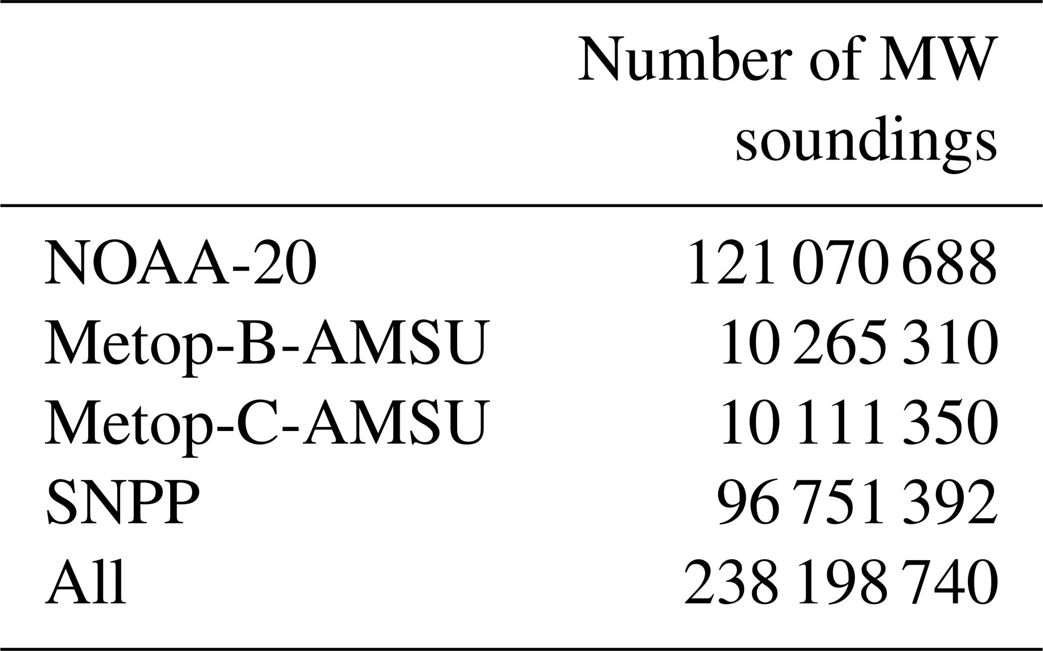
We devise a set of experiments to test the validity of the approximations of the rotation–collocation algorithm posed in the introduction and evaluate the computational efficiency gains for each. The experiments consist of a month of geolocations of actual RO data and nadir-scanning data from January 2021. Because of the promise in using nadir microwave radiance to construct weather-independent temperature and water vapor profiles from the surface to the stratopause, we use the geolocations of highly precise, well-calibrated microwave nadir radiance data. The nadir scanner geolocations are for the Advanced Microwave Sounding Unit (AMSU-A) instruments on the Metop satellites (Metop-B and Metop-C) and for the Advanced Technology Microwave Sounders (ATMS) on the Suomi-NPP and NOAA-20 satellites. All are in sun-synchronous orbits, with the Metop satellites having their ascending node at 21:31 LST (local solar time) and the Suomi-NPP and NOAA-20 satellites having theirs at 13:25 LST. In January 2021, all four of these microwave radiance instruments collected 238 198 740 soundings, as detailed in Table 1.
Table 1The total number of microwave radiance soundings over the month of January 2021 for each nadir-scanning microwave satellite.
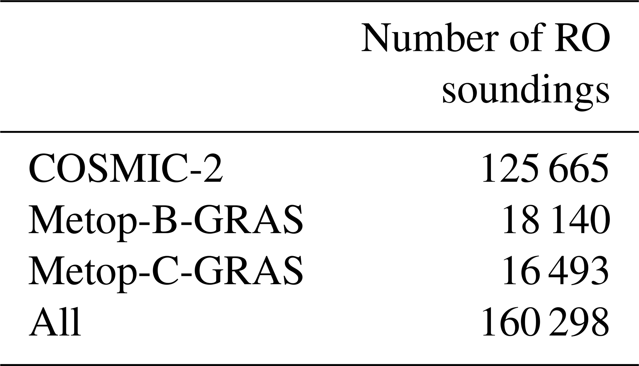
For the RO sounders, we choose two contemporary RO constellations: the two-satellite constellation of Metop consisting of Metop-B and Metop-C, and the six-satellite constellation of COSMIC-2. Note that the Metop satellites carry both nadir microwave scanners and RO instruments. These RO satellites are characterized by high signal-to-noise ratios for signal tracking but differ substantially in their orbits. The Metop satellites fly in sun-synchronous orbits, as above, while the COSMIC-2 satellites fly in 24∘ inclination, 520 km altitude, rapidly precessing orbits. In January 2021, the eight RO satellites obtained 160 298 RO soundings, as detailed in Table 2. By choosing these very different RO orbits, we can not only test the rotation–collocation algorithm but also gain some insight into the frequency of microwave–RO collocations according to orbit types. Co-hosted instruments such as on the Metop satellites can intuitively be expected to yield greater numbers of collocations daily than RO and microwave radiance instruments on different satellites with unrelated orbits – about 40 % of Metop RO soundings are collocated with Metop microwave radiance soundings, whereas generally under 5 % of RO soundings are collocated with microwave radiance soundings from any instrument hosted on a different satellite in an unrelated orbit. All computations are done in Python version 3.11. The orbit propagator used in computing u(t), i(t), and Ω(t) of Eq. (2a) is SGP4 (Vallado et al., 2006). It is initiated approximately three times daily from two-line orbit elements (TLEs). The transformation between ECF and ECI coordinate frames of Eq. (2b) is executed using astropy, with the ECF chosen to be the International Terrestrial Reference System (ITRS) and the ECI frame being the Geocentric Celestial Reference System (GCRS) (Price-Whelan et al., 2022). The conversion is executed only three times for every two-line element description in the Celestrak database in order to establish the Earth's pole and rotation rate. Subsequent transformations between ECF and ECI are executed using the calculated pole and rotation rate.
Table 2Total number of RO soundings over the month of January 2021 for each RO satellite. Note that the COSMIC-2 constellation contains six satellites. No Metop-C-GRAS soundings are available for 17 January 2021, so there are fewer Metop-C-GRAS soundings than Metop-B-GRAS soundings.
We obtained the Metop data from EUMETSAT (https://eoportal.eumetsat.int/, last access: 8 May 2023), and the NOAA-20 and Suomi-NPP data from NOAA's CLASS data system (https://www.class.noaa.gov/, last access: 8 May 2023). We retrieved the RO sounding data from the COSMIC Data Analysis and Archive Center (https://data.cosmic.ucar.edu/gnss-ro/, last access: 8 May 2023). We also retrieved historical TLEs for Suomi-NPP, Metop-B, Metop-C, NOAA-20, and the COSMIC-2 constellation from Celestrak (https://celestrak.org/, last access: 8 May 2023) for use in the rotation–collocation method. We grouped data into folders by instrument and day, and then ran all four methods on each combination of instruments per day.
We analyze the performance of the two approaches of the rotation–collocation algorithm using signal detection theory – counting false positive and false negative rates – using the brute-force algorithm as the definition of truth. Because the two approaches to the brute-force algorithm are provably the same despite their different approaches to checking for temporal matchups, they both yield precisely the same collocation pairs. In this section we present a set of case studies. In each case we choose a spatial tolerance of , and in all cases but the last we choose a time window of Δt = 600 s, or 10 min; in the fourth and final case we choose a time window of Δt = 10 800 s, or 3 h. Occultation yield can be expected to increase in direct proportion to Δt for time windows significantly shorter than the orbital period of the nadir-scanning satellites. The first case study considers collocations between COSMIC-2 RO soundings and NOAA-20 microwave radiance soundings. This is a typical case since many future RO instruments will not necessarily be co-hosted with microwave radiance sounders and will be in different orbits. The second case study is for the co-hosted RO and microwave radiance soundings on the Metop satellites. While not many such pairings will be deployed in the future, it may suggest that RO and microwave radiance sounders be flown in tandem orbits if maximizing the collocation yield is desired. Third, the total yield of RO–microwave radiance collocations for the month of January 2021 is considered. The final case study reconsiders collocations between COSMIC-2 RO soundings and NOAA-20 microwave radiance soundings but with a time window of Δt = 10 800 s. This final case study demonstrates the excellent accuracy and efficiency of the rotation–collocation method with sub-occultations over long time windows and documents the slight decrease in accuracy of the linearized rotation–collocation method as the curvature of the trajectory of sub-occultations in the nadir scanner frame increases over a longer time window.
4.1 Case study: COSMIC-2 (RO) and NOAA-20 (microwave)
In this case study, we examine collocations between the six-satellite COSMIC-2 radio occultation constellation and ATMS on NOAA-20, a microwave radiance sounder. In Fig. 2a, we show the collocations between COSMIC-2 and NOAA-20 by day found for each of our four collocation-finding methods. Both brute-force methods yield identical results, and so both methods are represented in Fig. 2a by the same blue line. The rotation–collocation algorithm with sub-occultations (orange) and the linearized rotation–collocation algorithm (light green) find slightly more collocations on each day than the brute-force algorithms (blue), but the true positive rate, defined as the number of collocations correctly predicted by the rotation–collocation method divided by the total number of correctly or incorrectly predicted collocations, is over 98.5 % for both versions of the rotation–collocation method. The time window for collocation for Fig. 2 is Δt = 600 s. The “fraction collocated” axis on the right of Fig. 2a is the number of predicted collocations divided by the average number of daily occultations. Notably, only 2 % to 5 % of COSMIC-2 RO soundings are collocated with NOAA-20 ATMS microwave radiance soundings over the month of January 2021 when Δt=600 is used as the time tolerance for collocation because NOAA-20 and COSMIC-2 satellites are rarely near each other.
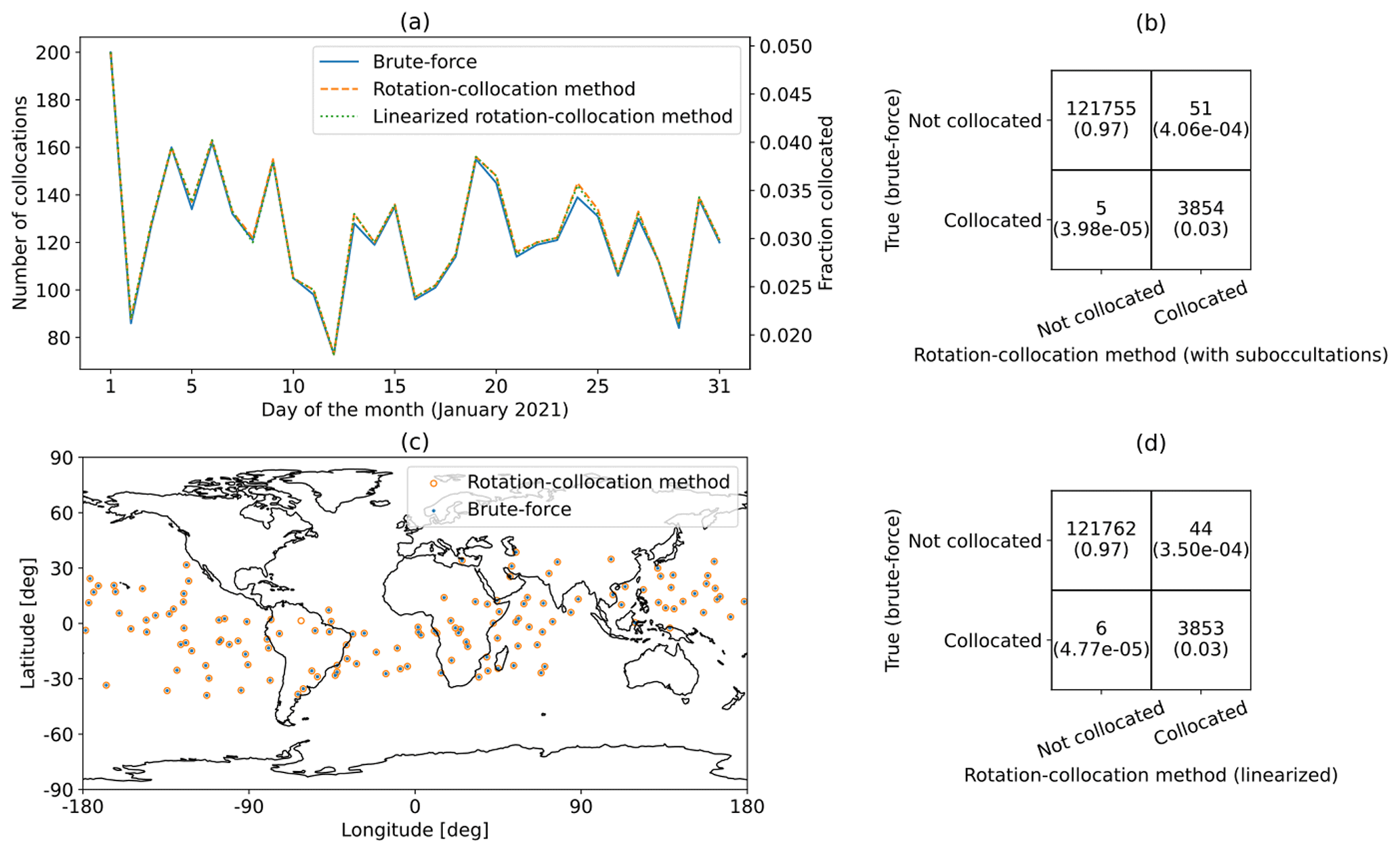
Figure 2(a) Daily collocations for COSMIC-2 RO soundings and NOAA-20 ATMS microwave radiance soundings for the month of January 2021. (b) Confusion matrix for the COSMIC-2 RO soundings and NOAA-20 ATMS microwave soundings for January 2021 for the rotation–collocation method with sub-occultations. (c) Map of collocations on 15 January 2021 for NOAA-20 ATMS soundings and COSMIC-2 RO soundings. (d) Confusion matrix for the COSMIC-2 RO soundings and NOAA-20 ATMS microwave soundings for January 2021 for the linearized rotation–collocation method.
In Fig. 2b, we show a confusion matrix for this case study. The number of sub-occultations used for this analysis is N=21, and the temporal spacing between sub-occultations is dt = 60 s. In the confusion matrix, the top and bottom rows correspond to the numbers of collocations of RO soundings not found and found by brute force, respectively, and the left and right columns correspond to the numbers of collocations of RO soundings not predicted and predicted by one of the rotation–collocation methods, respectively. The true positive rate for the rotation–collocation method with sub-occultations is 3854 3905 = 98.7 % and the true negative rate is 121 755 121 760 = 99.996 %.
In Fig. 2c, we show the spatial distribution of COSMIC-2 soundings collocated with NOAA-20 microwave radiance soundings for 15 January 2021 found by the linearized rotation–collocation algorithm and by the brute-force method. Collocations found by the linearized rotation–collocation algorithm are shown as orange circles, while those found by the brute-force algorithm are shown as blue dots. The vast majority of these collocated soundings are found by both methods. The brute-force algorithm found 135 collocations, and the rotation–collocation algorithm found 136 collocations – the same 135 collocations found by the brute-force algorithm plus an extra collocation. For this day, the true positive rate is 135 136 = 99.3 %.
In Fig. 2d, we show a confusion matrix for collocations found by the linearized rotation–collocation algorithm between COSMIC-2 RO soundings and NOAA-20 ATMS soundings for the month of January 2021. The linearized rotation–collocation algorithm finds the same collocations as the rotation–collocation method with sub-occultations in this case, and so the true positive rate for the linearized rotation–collocation method is 3853 3897 = 98.9 %, while the true negative rate is 121 762 121 768 = 99.995 %.
Many of the COSMIC-2 RO soundings misclassified by the linearized rotation–collocation method (44 out of 50 total) are incorrect predictions, predicting a collocation when one does not exist. We found that 7 (15.9 % of total) are soundings that fall just outside the time window Δt. This occurs when one endpoint of the apparent RO scan pattern in the coordinate frame given by NOAA-20's orbit lies close to, but does not cross, the δu=0 line. The remaining 37 false positives (84.1 % of total) are soundings that fall just outside of the maximum scan range δs of the NOAA-20 ATMS instrument. One such false positive is pictured in Fig. 3.
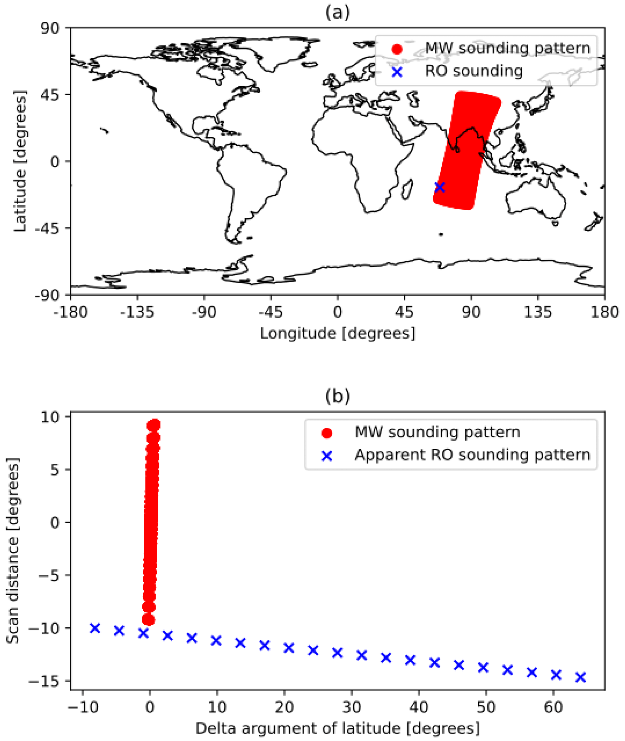
Figure 3(a) A radio occultation from COSMIC-2, occurring at 07:55:12 GMT on 3 January 2021, falsely identified by the rotation–collocation method as a collocation, plotted against contemporaneous MW soundings from NOAA-20 ATMS. (b) The discretized apparent position of the same occultation rotated into the MW frame, plotted against the MW sounding pattern.
All of the false positive and false negative cases found here are associated with failures of the first assumption of the rotation–collocation algorithm, which is all of the nadir scanner soundings fall perfectly on an unbroken line at δu=0 in the rotated frame as illustrated by Fig. 1c. There are more false positives than false negatives because of our windowing criteria, and adjusting these criteria would lead to more false negatives but fewer false positives. All the false positives and false negatives occur very close to the spatial or temporal boundaries for collocation, and so these misclassified soundings represent low-value collocations compared to other soundings that have more temporal and spatial overlap with the nadir scanner sounding pattern.
In summary, the rotation–collocation algorithm with sub-occultations is correct on 98.7 % of the occasions for which a collocation between COSMIC-2 RO soundings and NOAA-20 ATMS soundings is predicted and incorrect only 0.004 % of the time when a COSMIC-2 RO sounding is not found to be collocated with a NOAA-20 ATMS sounding. The linearized rotation–collocation algorithm is correct on 98.9 % of the occasions for which a collocation between COSMIC-2 RO soundings and NOAA-20 ATMS soundings is predicted and incorrect only 0.005 % of the time when a COSMIC-2 RO sounding is not found to be collocated with a NOAA-20 ATMS sounding. Over the course of January 2021, the true number of collocated soundings between COSMIC-2 RO and NOAA-20 ATMS soundings within a time window of 10 min is 3859. The yield as a fraction of total COSMIC-2 RO soundings is 3.1 % over the month. On a daily basis, the fraction ranges from 2.0 % to 5.0 %; see Fig. 2a.
4.2 Case study: Metop-B (RO) and Metop-B (microwave)
In this case study, we examine collocations between two instruments co-hosted on a satellite, the GRAS RO instrument and the AMSU-A nadir-scanning microwave radiance instrument. Figure 4 is the same as Fig. 2 but for this case study.
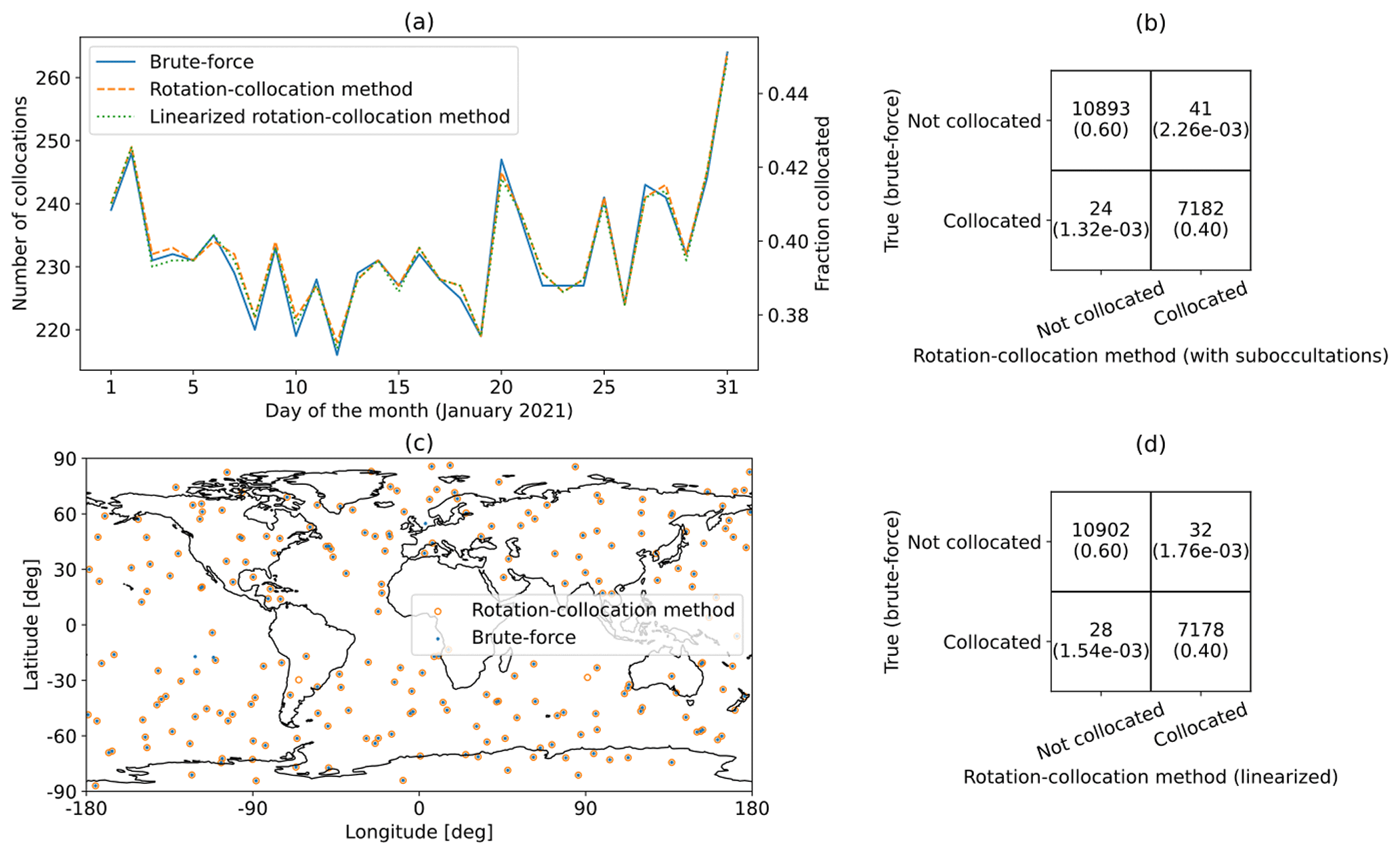
Figure 4(a) Daily collocations for Metop-B GRAS RO soundings and Metop-B AMSU-A microwave radiance soundings for the month of January 2021. (b) Confusion matrix for the Metop-B GRAS RO soundings and Metop-B AMSU-A ATMS microwave soundings for January 2021 for the rotation–collocation method with sub-occultations. (c) Map of collocations on 15 January 2021 for Metop-B AMSU-A microwave soundings and Metop-B GRAS RO soundings. (d) Confusion matrix for the Metop-B GRAS RO soundings and Metop-B AMSU-A microwave soundings for January 2021 for the linearized rotation–collocation method.
Co-hosting instruments greatly increases the collocation yield, with around 38 %–46 % of Metop-B RO soundings collocated with Metop-B microwave soundings, in comparison to around 3 % of COSMIC-2 RO soundings collocated with NOAA-20 microwave soundings. The intuition for this is straightforward. If a setting RO sounding is obtained at a time tRO, then it is very likely that the satellite had flown over that same location earlier by in which L is the limb distance for the RO sounding and vleo is the low-Earth-orbiting satellite's orbital velocity. Typically, L≃3000 km and vleo≃7.5 km s−1, meaning a collocated microwave radiance sounding may have been swept out by the scanner approximately 400 s prior. The temporal collocation check is always satisfied for co-hosted RO and nadir-scanning instruments as long as the spatial window is greater than 400 s (Δt>400 s). For the collocation to be found, though, the boresight angle of the RO sounding with respect to the satellite's velocity vector must be less than the angle corresponding to the sweep of the AMSU-A scan δsmax as viewed at limb distance L. Maximum boresight angles for RO instruments typically lie around 60∘, but the nadir scan of AMSU-A corresponds to a maximum boresight of approximately 27∘ at limb distance. As a consequence, instead of all RO soundings by Metop-B being collocated with a Metop-B microwave sounding, approximately only 40 % are collocated in this way. This corresponds to the spatial check for collocation only being met 40 % of the time.
Figure 4b shows the performance of the rotation–collocation method with sub-occultations on collocations between Metop-B-GRAS and Metop-B-AMSU throughout the month of January 2021 using 21 sub-occultations or a 60 s spacing between sub-occultations. The true positive rate for the rotation–collocation method with sub-occultations is 7182 7223 = 99.4 %, and the true negative rate for the rotation–collocation method with sub-occultations is 10 893 10 917 = 99.8 %.
Figure 4d shows the performance of the linearized rotation–collocation method on collocations between Metop-B-GRAS and Metop-B-AMSU throughout the month of January 2021. Most of the Metop-B-GRAS soundings misclassified by the linearized rotation–collocation method are false positives. We have found that 2 of 32 (6.25 %) of the false positives are due to unavailable Metop-B-AMSU data – for these predicted collocations, there are no Metop-B-AMSU sounding data available within 8 s of the predicted collocation time. The remaining 30 (93.75 % of total) false positives are soundings that fall just outside of the maximum scan range δumax of the Metop-B-AMSU instrument. The true positive rate for the linearized rotation–collocation method is 7178 7210 = 99.6 %, and the true positive rate increases slightly to 7178 7208 = 99.6 % when excluding incorrect predictions that occur due to missing data. The true negative rate for the rotation–collocation method is 10 902 10 930 = 99.7 %.
4.3 Full analysis: COSMIC-2 and Metop (RO) and S-NPP, NOAA-20, and Metop (MW)
In this section, we examine collocations between COSMIC-2 and Metop-B and Metop-C radio occultations and Metop, S-NPP, and NOAA-20 microwave soundings. In Fig. 5a, we show the collocations by day found by each of our four collocation-finding methods, as well as the fraction of radio occultations that are collocated with microwave soundings, using the daily average number of radio occultations as the denominator. Metop-C-GRAS data were missing for 17 January, which explains the steep drop in total collocations found on 17 January. As before, the time window for collocation is Δt=600 s.
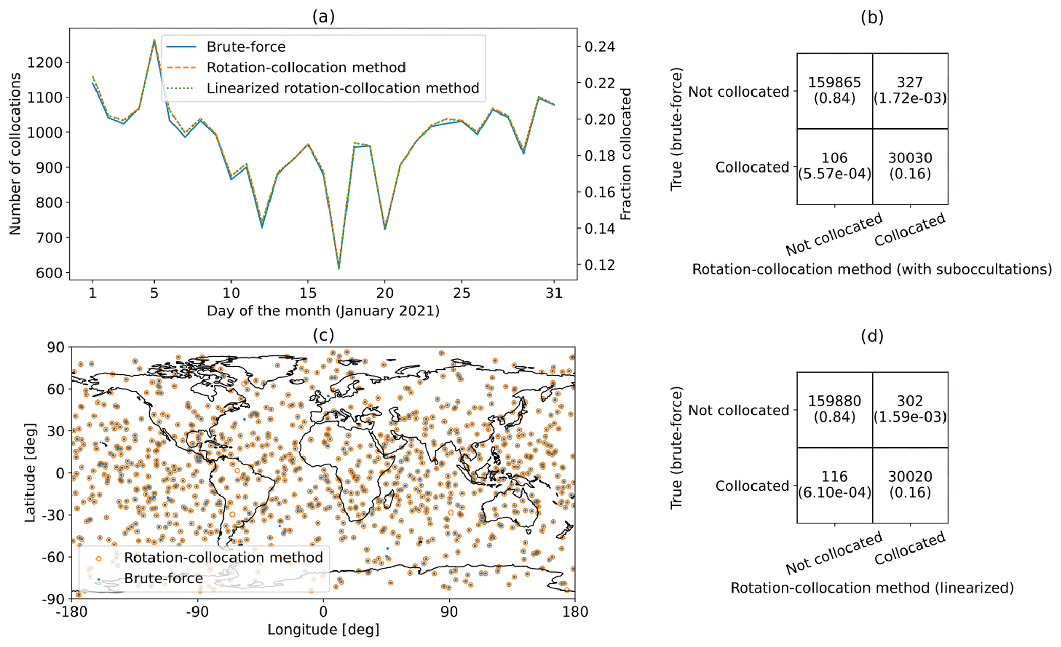
Figure 5(a) Daily collocations for all satellite combinations for the month of January 2021. (b) Confusion matrix for all satellite combinations for January 2021 for the rotation–collocation method with sub-occultations. (c) Map of collocations on 15 January 2021 for all satellite combinations. (d) Confusion matrix for all satellite combinations for January 2021 for the linearized rotation–collocation method.
Over all satellite combinations, only 15.8 % of RO soundings are collocated with any MW soundings; ideally, as many RO soundings would be collocated with MW soundings as possible. It is clear that there is room for improvement in the percentage of soundings that are collocated, and co-hosting instruments leads to a large increase in collocations, as shown in Sect. 4.2.
In Fig. 5c, we show all the collocations on 15 January 2021. These collocations occur all over the globe. Collocations in the tropics, between 23.43∘ S and 23.43∘ N in latitude, are most important for profiling water vapor in the planetary boundary layer (Wang et al., 2017). Future satellite missions with GNSS-RO payloads should consider co-hosting microwave radiometer payloads or launching into low-inclination orbits in order to meet the need for collocations in the tropics.
Overall, the linearized rotation–collocation method found 30 020 collocations and correctly identified 159 880 RO soundings as not collocated. There were 116 missed predictions or occultations for which the brute-force method found a collocation but the linearized rotation–collocation method did not. There were 302 incorrect predictions, which are occultations where the linearized rotation–collocation method found a collocation, but the brute-force method did not. Out of these 302 incorrect predictions, 44 (14.6 % of total) were caused by missing microwave data, 85 (28.1 % of total) were soundings that fall just outside of the maximum scan range of an microwave instrument, and the remaining 173 (57.3 % of total) were soundings that fall just beyond the maximum delta argument of latitude when compared to an MW satellite's orbit. The linearized rotation–collocation method had a 30 020 30 322 = 99.0 % true positivity rate and a 159 880 159 996 = 99.9 % true negative rate. Excluding incorrect predictions resulting from missing or corrupted microwave radiance data, the true positive rate is 30 020 30 278 = 99.1 %.
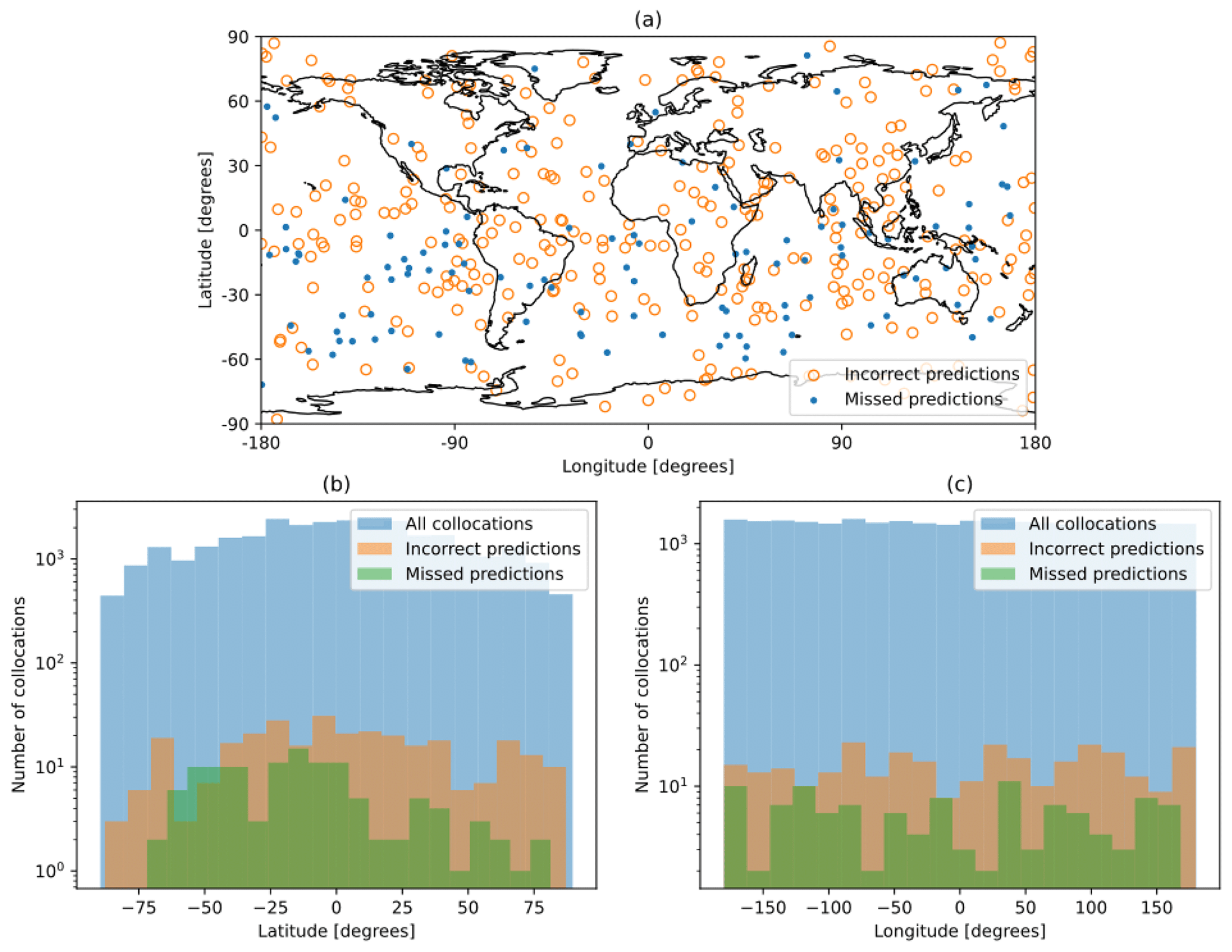
Figure 6(a) Map of incorrect and missed predictions for all satellite combinations. (b) Histogram of latitude of all collocations, incorrect predictions, and missed predictions for all satellite combinations. (c) Histogram of longitude of all collocations, incorrect predictions, and missed predictions for all satellite combinations.
Figure 6a shows the geographic distribution of incorrect predictions and missed predictions. Figure 6b and c display the distribution of latitude and longitude, respectively, for incorrect predictions, missed predictions, and all collocations. The set of all collocations is roughly centered at the Equator and prime meridian, with a mean latitude of 0.49∘, mean longitude of −1.69∘, standard deviation of latitude of 42.2∘, and standard deviation of longitude of 104.1∘. The distribution of incorrect predictions is similar, with a mean latitude of 2.82∘, mean longitude of 4.52∘, standard deviation of latitude of 42.2∘, and standard deviation of longitude of 103.4∘. The distribution of missed predictions, however, is centered slightly south of the Equator; it has a mean latitude of −12.58∘, mean longitude of −10.5∘, standard deviation of latitude of 34.1∘, and standard deviation of longitude of 105.4∘. The sample size (n=116) of missed predictions is small, however, which makes it difficult to evaluate the significance of this small shift in geographic distribution.
4.4 Number of collocations by day for each satellite combination
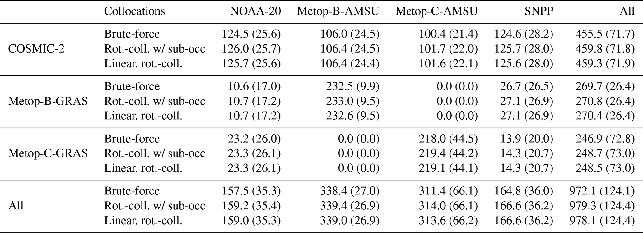
Table 3 shows the number of collocations per day over the month of January 2021 for each satellite combination. Metop-B-AMSU and Metop-B-GRAS generate a large yield of collocations. These instruments are co-hosted, which allows a high percentage of occultations to be collocated with microwave soundings. For the same reason, Metop-C-AMSU and Metop-C-GRAS share a high number of collocations. There are no collocations between Metop-B-AMSU and Metop-C-GRAS and none between Metop-C-AMSU and Metop-B-GRAS. Metop-B and Metop-C have co-planar orbits but are approximately half an orbit apart within their orbital plane. As such, their trajectories never intersect or get sufficiently close for measurements from their instruments to be collocated.
Table 3Number of collocations by day, using Δt=600 s as the temporal criterion and Δd=150 km as the spatial criterion for collocation, for each satellite combination. The first row in each cell shows the average number of collocations per day found by both brute-force methods (recall that both brute-force methods yield an identical list of collocations), with the standard deviation of the number of collocations per day in parentheses. The second row shows the same metrics for the rotation–collocation method with sub-occultations, and the third row shows the same metrics for the linearized rotation–collocation method.
4.5 Computational expense analysis and accuracy
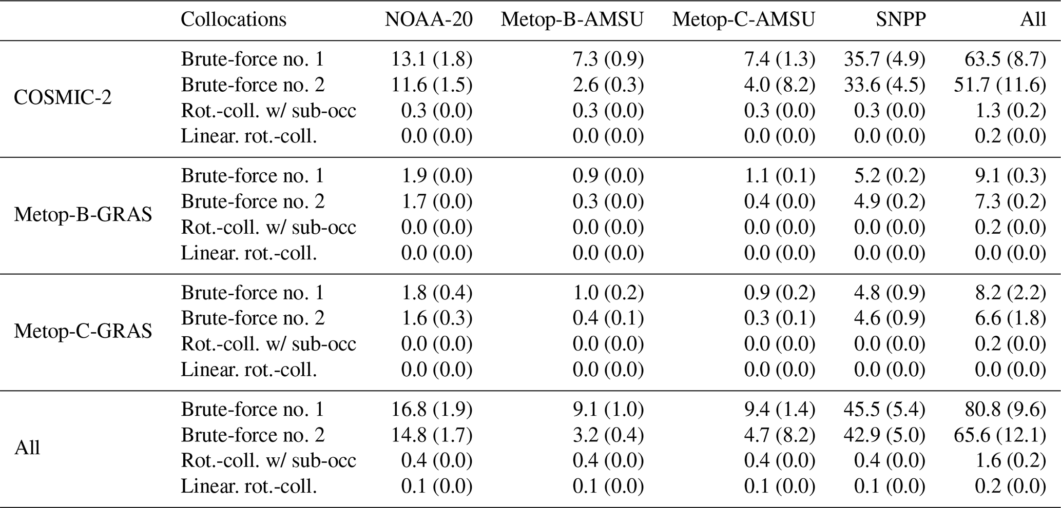
Table 4 shows the core minutes per day of RO data required to compute collocations for different combinations of satellites on an eight-core 2020 MacBook Pro with an M1 chip and 16 GB of RAM. The fastest method, the linearized rotation method, takes on average less than a single core minute per day to compute collocations for all satellites and achieves a 328-fold acceleration over the sorted brute-force method. The acceleration by the linearized rotation–collocation method varies depending on the time tolerance and computational hardware used but in general ranges between 40-fold and 400-fold over conventional brute-force algorithms.
Table 4Core minutes required for computation by day, using Δt=600 s as the temporal criterion and Δd=150 km as the spatial criterion for collocation, for each satellite combination (excluding data-loading). The first row in each cell shows the average core minutes required to compute the collocations for a satellite pair for a single day using brute-force method no. 1, with the standard deviation of core minutes taken for computation time in parentheses. The second row shows the same metrics for the sorted brute-force method, the third row shows the same metrics for the rotation method with sub-occultations, and the fourth row shows the same metrics for the linearized rotation–collocation method.
4.6 Longer timescale analysis
Recall the second assumption outlined in Sect. 2.2: the apparent position of an RO sounding in a nadir sounder frame forms a linear trajectory. Over longer timescales, this trajectory elongates and its curvature becomes more apparent. To test the validity of this assumption, we applied all four collocation-finding methods to finding collocations between NOAA-20 ATMS and COSMIC-2 with Δt=3 h, a time window 18 times longer than that used for Sect. 4.1–4.5. Increasing the time tolerance in this way greatly increases the number of possible collocations. For the rotation–collocation method with sub-occultations, we used N=5 sub-occultations or a spacing of dt=5400 s between sub-occultations.
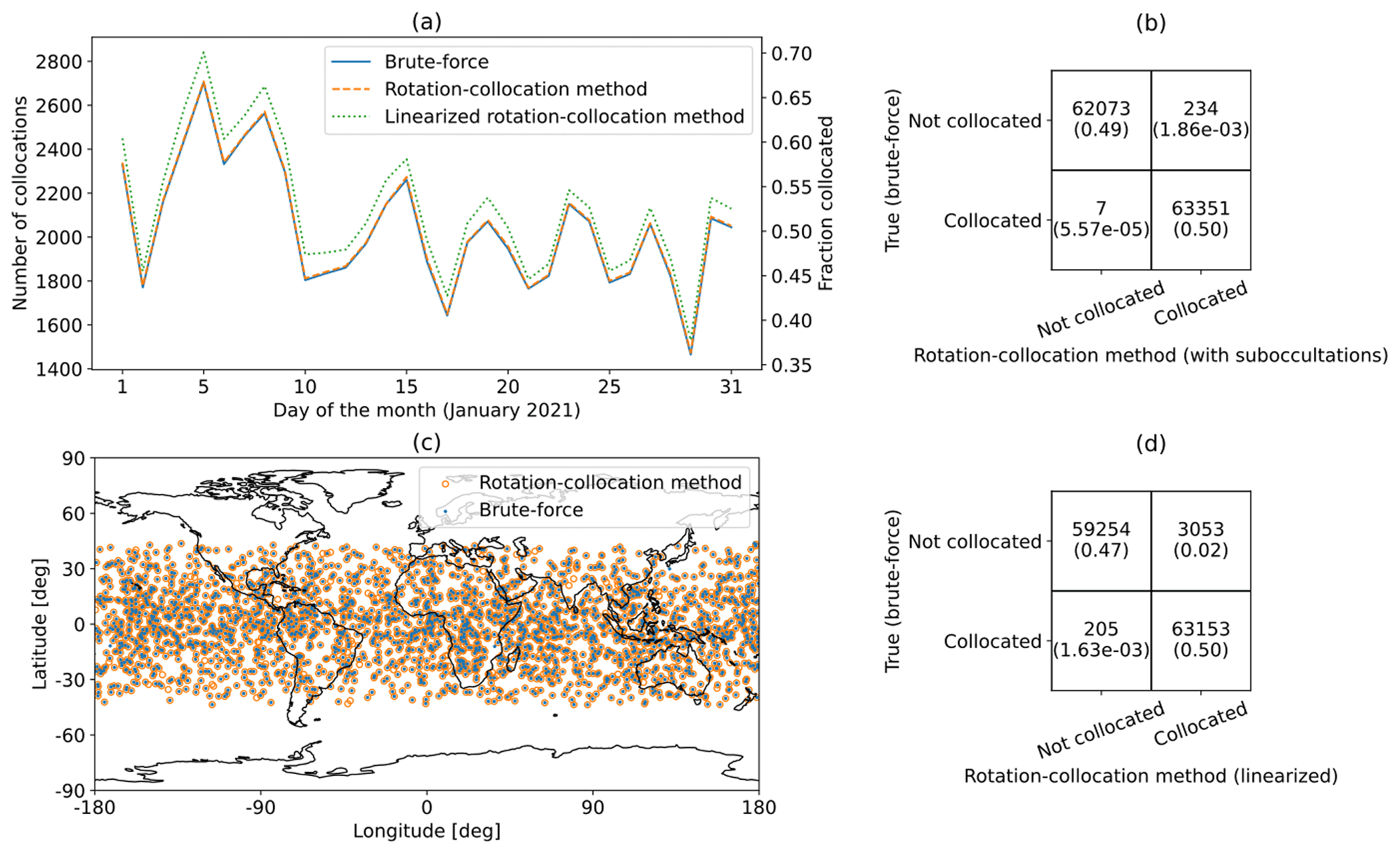
Figure 7(a) Daily collocations for COSMIC-2 RO soundings and NOAA-20 ATMS microwave radiance soundings for the month of January 2021, with a 3 h time tolerance. (b) Confusion matrix for the COSMIC-2 RO soundings and NOAA-20 ATMS microwave soundings for January 2021 for the rotation–collocation method with sub-occultations. (c) Map of collocations on 15 January 2021 for NOAA-20 ATMS soundings and COSMIC-2 RO soundings. (d) Confusion matrix for the COSMIC-2 RO soundings and NOAA-20 ATMS microwave soundings for January 2021 for the linearized rotation–collocation method.
Figure 7a shows the collocations by day on the left vertical axis and fractional yield of collocations on the right vertical axis for NOAA-20 and COSMIC-2 over January 2021. With Δt=10 800 s (3 h), the linearized rotation–collocation method (light green) finds many more collocations than the brute-force algorithm (blue) and the rotation–collocation method with sub-occultations (orange). It is also apparent that with a time window of 3 h, around half of all COSMIC-2 RO soundings are collocated with NOAA-20 soundings, many more than with a time window of 10 min.
Figure 7b shows the performance of the rotation–collocation method with sub-occultations on collocations between COSMIC-2 and NOAA-20 for January 2021. This method has a true positive rate of 63 351 63 585 = 99.6 % and a true negative rate of 62 073 62 080 = 99.99 %. Figure 7d shows the performance of the linearized rotation–collocation method on collocations between COSMIC-2 and NOAA-20 for January 2021. This method has a true positive rate of 63 153 66 206 = 95.4 % and a true negative rate of 59 254 59 459 = 99.7 %.
Table 5Total number of incorrect predictions (collocations identified by the rotation–collocation method but not by the brute-force method), total number of missed predictions (collections missed by the rotation–collocation method but found by the brute-force method), and total number of correct predictions (collocations found by both methods) for collocations between NOAA-20 ATMS soundings and COSMIC-2 RO soundings over the month of January 2021 with a 3 h time tolerance for collocation for the rotation–collocation method evaluated with a varying number of sub-occultations.
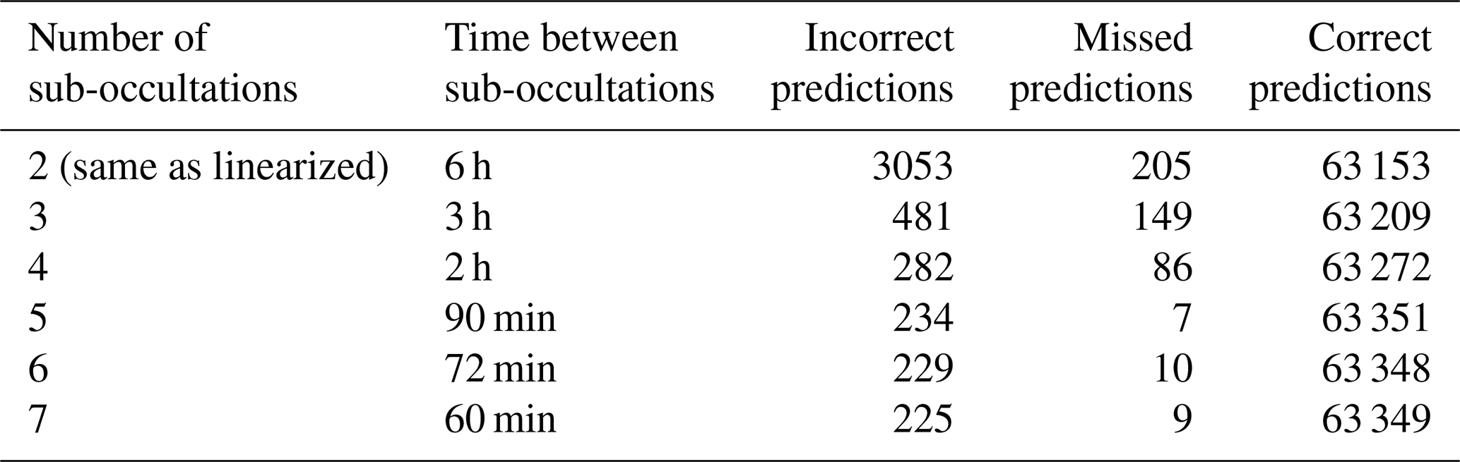
Although the linearized rotation–collocation method has many more incorrect predictions than the rotation–collocation method with sub-occultations, it retains a 95.4 % true positive rate. This illustrates that even over a 3 h period, the linearization of the trajectory of the apparent RO sounding in the nadir sounder frame is good enough to maintain a high level of accuracy. Also notable is that the sub-occultations used in this case study are spaced 90 min apart, longer than the 20 min spacing between endpoints used by the linearized rotation method in Sect. 4.1–4.5. Even so, with a 90 min spacing between sub-occultations, there is a true positive rate of 99.9 % and only 234 incorrect predictions and 7 missed predictions for collocations between NOAA-20 and COSMIC-2 over the month of January 2021, which is better than the true positive rate of 98.9 % found with a 20 min spacing between sub-occultations for collocations between NOAA-20 and COSMIC-2 in Sect. 4.1. A 90 min spacing between sub-occultations is sufficient to achieve the accuracy demonstrated in Sect. 4.1–4.5; longer time windows between sub-occultations result in more incorrect and missed predictions and reduced accuracy, as demonstrated in Table 5. The correlation between time between sub-occultations and accuracy breaks down as sub-occultations get close enough in time that the trajectory of the apparent RO sounding in the nadir sounder frame becomes approximately linear, at which point adding sub-occultations increases computation time without improving performance. This phenomenon can be seen in Table 5 – accuracy greatly improves as more sub-occultations are added, up to N=5 sub-occultations, after which point performance remains relatively consistent.
Even with Δt=3 h, the rotation–collocation method remains extremely fast. On average, the brute-force method took 156.2 core minutes to compute collocations for a single day of COSMIC-2 RO data, and the sorted brute-force method took 155.5 core minutes to compute a day's worth of collocations. In contrast, the rotation–collocation method with sub-occultations took just 0.09 core minutes to compute a day's worth of collocations and the linearized rotation–collocation method took 0.05 core minutes on average to compute a day's worth of collocations. This results in a 3124-fold acceleration by the linearized rotation–collocation method over the brute-force method and a 1735-fold acceleration by the rotation–collocation method with sub-occultations over the brute-force method.
The apparent computational efficiency gains come about because the brute-force methods are decelerated more rapidly than (Δt)−1 with longer time tolerance Δt. Brute-force methods only do the spatial check for nadir scan soundings that match in time, and so when many more soundings match in time, many more spatial checks are performed, which can be quite slow. This problem is particularly acute for the sorted brute-force method, which is actually the slowest method for a time window of 3 h. The key advantage of the sorted brute-force method is that it considers many fewer nadir scanner soundings for each RO sounding than brute-force method no. 1 does. When the time window is long, this advantage evaporates, but the time taken to search for the start and end of the time window in the sorted list of soundings remains, making the time taken by the sorted brute-force method similar to that taken by the brute-force method no. 1.
Additionally, because some RO soundings may occur at the very beginning or very end of a day, the brute-force methods must consider 30 h of nadir scanner sounding, beginning 3 h before the start of the day and ending 3 h after the end of day, in order to find all collocations for a single day. With a 10 min time tolerance for collocations, the brute-force methods only need consider 24 h and 20 min of microwave soundings, speeding up the search for collocations. As a result, the acceleration provided by the rotation–collocation method is much more dramatic with Δt=3 h than with Δt=10 min.
In conclusion, the rotation–collocation method retains remarkable accuracy when the time spacing between sub-occultations is 90 min or less. Even with a 3 h spacing between sub-occultations, the rotation–collocation method retains an accuracy above 95 %. The time taken by the rotation–collocation method only scales with number of RO soundings and number of sub-occultations, whereas the time taken by the brute-force method scales with time tolerance. This makes the rotation–collocation method an excellent choice for finding collocations with time tolerances of 3 h or more.
The rotation–collocation method has great potential to quickly find collocations between RO soundings and nadir scan soundings. In fact, the rotation–collocation method generalizes easily and can be applied to any set of sparsely sampled satellite data and any set of continuously sampled data from a nadir-scanning satellite. When applied to a month's worth of RO soundings from COSMIC-2, Metop-B-GRAS, and Metop-C-GRAS and a month's worth of MW soundings from Metop-B-AMSU, Metop-C-AMSU, SNPP, and NOAA-20 with a time tolerance of 10 min, the linearized rotation–collocation method finds 30 020 collocations with a 99.0 % true positive rate and a 99.9 % true negative rate and has a 328-fold acceleration over the brute-force method. Furthermore, when incorrect predictions that result from missing microwave are held out, the linearized rotation–collocation method achieves a true positive rate of 99.1 %. This indicates that when the time tolerance for collocation is low, the linearized rotation–collocation method achieves near-perfect accuracy and does so hundreds of times faster than the fastest brute-force method.
When applied to a months' worth of COSMIC-2 RO soundings and NOAA-20 microwave soundings with a 3 h time tolerance for collocation, the rotation–collocation method with sub-occultations spaced 90 min apart achieves 99.6 % true positive and 99.9 % true negative rates with a 1735-fold acceleration over the fastest brute-force method. The linearized rotation–collocation method achieves 95.4 % true positive and 99.6 % true negative with a 3124-fold acceleration over the brute-force method. This demonstrates that the rotation–collocation method maintains a near-perfect accuracy with sub-occultations up to an hour apart and that the rotation–collocation methods offer an improvement in speed over brute-force methods as the time tolerance for collocation is increased.
Currently, the geographic distribution of the soundings misclassified by the rotation–collocation algorithm roughly matches the geographic distribution of collocated soundings, as shown in Fig. 6. Furthermore, most misclassified soundings are incorrect predictions (collocations predicted by the rotation–collocation algorithm but not by the brute-force method). Incorrect predictions can be easily debunked, as the rotation–collocation algorithm currently predicts the expected time and scan angle of the collocated nadir scanner sounding for each collocation, and it is computationally trivial to check if a real nadir scanner sounding exists at the expected time and scan angle.
Finally, the rotation–collocation method shows that with a 10 min time tolerance and 150 km spatial tolerance, there were an average of nearly 1000 collocated RO soundings each day of January 2021 or around 16 % of all unique RO soundings from Metop-B-GRAS, Metop-C-GRAS, and COSMIC-2. Around 40 % of Metop-B-GRAS soundings were collocated with Metop-B-AMSU soundings, and around 40 % of Metop-C-GRAS soundings were collocated with Metop-C-AMSU soundings. Co-hosted instruments on Metop-B and Metop-C greatly increase the percentage of soundings that are collocated, and co-hosting MW and RO instruments is a powerful tool for increasing the number of collocations.
Future work and applications
At present, the rotation–collocation algorithm identifies RO soundings which are collocated with nadir scanner soundings and additionally identifies the expected time and scan angle of the presumably collocated nadir scanner sounding. However, the rotation–collocation algorithm does not verify the existence of a nadir scanner sounding at the expected time and scan angle, and thus it does not extract the specific nadir scanner soundings associated with each collocation. The brute-force algorithms implemented in this paper also do not identify the specific nadir scanner soundings associated with each collocation. In the future, the authors plan to extend the rotation–collocation algorithm to identify the specific nadir scanner soundings associated with each collocated RO sounding and to integrate this extended version of the rotation–collocation algorithm into NASA's existing Earth science data management software in order to speed up finding of collocations and the assimilation of RO data into numerical weather prediction models.
The authors anticipate that extracting specific nadir scanner soundings associated with each collocation will slow down both the rotation–collocation and brute-force methods but will narrow the performance gap between the rotation–collocation and brute-force methods. Nevertheless, the authors expect that the rotation–collocation method will remain much faster than equivalent brute-force methods. The authors also plan to further investigate the geographic distribution of collocations missed by the rotation–collocation method.
The rotation–collocation method can be easily modified to identify collocations between two different nadir-scanning satellites. It can also be extended to predict collocation yield for satellite missions with nadir-scanning payloads in different orbits. In this way, the rotation–collocation method can be used as a constellation planning tool and a mission planning tool in order to select collocation-maximizing orbits for nadir-scanning satellites.
The code associated with this paper is available at https://github.com/alexmeredith8299/ro-nadir-collocation (last access: 8 May 2023; https://doi.org/10.5281/zenodo.7908115, Meredith, 2023). All of the data associated with this paper are freely available from UCAR (https://doi.org/10.5065/1k0w-2272, UCAR, 2023; https://doi.org/10.5065/t353-c093, UCAR COSMIC Program, 2019), NOAA (https://www.avl.class.noaa.gov, NOAA, 2023), EUMETSAT (https://eoportal.eumetsat.int, login required, EUMETSAT, 2023), and Celestrak (https://celestrak.org/satcat/search.php, Kelso, 2023). The code repository contains instructions on how to download the data.
AM performed data analysis and contributed to the manuscript. SL designed the study, provided advice on data analysis, and contributed to the manuscript. LH performed data analysis. KC provided advice on data analysis and on the manuscript. All authors contributed to the interpretation of the results and edited the manuscript.
The contact author has declared that none of the authors has any competing interests.
Any opinion, findings, and conclusions or recommendations expressed in this material are those of the
authors(s) and do not necessarily reflect the views of the National Science Foundation.
Publisher's note: Copernicus Publications remains neutral with regard to jurisdictional claims in published maps and institutional affiliations.
This research has been supported by the Directorate for Geosciences, Division of Atmospheric and Geospace Sciences (grant no. GEO-1850089), the NASA Decadal Survey Incubator Program (grant no. 80NSSC22K1103), and the NSF Graduate Research Fellowship Program (grant no. 2141064).
This paper was edited by Peter Alexander and reviewed by two anonymous referees.
Banos, I., Sapucci, L., Cucurull, L., Bastarz, C., and Silveira, B.: Assimilation of GPSRO Bending Angle Profiles into the Brazilian Global Atmospheric Model, Remote Sens., 11, 256, https://doi.org/10.3390/rs11030256, 2019. a
Cardinali, C. and Healy, S.: Impact of GPS radio occultation measurements in the ECMWF system using adjoint-based diagnostics, Q. J. Roy. Meteor. Soc., 140, 2315–2320, https://doi.org/10.1002/qj.2300, 2014. a
Chung, N., Cram, T., Smith, S. R., Tsontos, V. M., Huang, T., Sparling, K., Perez, S., Phyo, W., Ji, Z., and Kuttruff, R.: Development of a Cloud-based Data Match-Up Service (CDMS) in Support of Ocean Science Applications, in: OCEANS 2022, Hampton Roads, 1–6, https://doi.org/10.1109/OCEANS47191.2022.9977163, 2022. a
EUMETSAT: AMSU-A Level 1B – Metop – Global, European Organisation for the Exploitation of Meteorological Satellites, https://eoportal.eumetsat.int, last access: 8 May 2023. a
Feltz, M., Knuteson, R., and Revercomb, H.: Assessment of COSMIC radio occultation and AIRS hyperspectral IR sounder temperature products in the stratosphere using observed radiances, J. Geophys. Res., 122, 8593–8616, https://doi.org/10.1002/2017JD026704, 2017. a
Gelaro, R., McCarty, W., Suárez, M., Todling, R., Molod, A., Takacs, L., Randles, C., Darmenov, A., Bosilovich, M., Reichle, R., Wargan, K., Coy, L., Cullather, R., Draper, C., Akella, S., Buchard, V., Conaty, A., da Silva, A., Gu, W., Kim, G., Koster, R., Lucchesi, R., Merkova, D., Nielsen, J., Partyka, G., Pawson, S., Putman, W., Rienecker, M., Schubert, S., Sienkiewicz, M., and Zhao, B.: The Modern-Era Retrospective Analysis for Research and Applications, version 2 (MERRA-2), J. Climate, 30, 5419–5455, 2017. a
Healy, S. and Eyre, J.: Retrieving temperature, water vapour and surface pressure information from refractive-index profiles derived by radio occultation: A simulation study, Q. J. Roy. Meteor. Soc., 126, 1661–1683, https://doi.org/10.1002/qj.49712656606, 2000. a
Hersbach, H., Bell, B., Berrisford, P., Hirahara, S., Horányi, A., Muñoz Sabater, J., Nicolas, J., Peubey, C., Radu, R., Schepers, D., Simmons, A., Soci, C., Abdalla, S., Abellan, X., Balsamo, G., Bechtold, P., Biavati, G., Bidlot, J., Bonavita, M., De Chiara, G., Dahlgren, P., Dee, D., Diamantakis, M., Dragani, R., Flemming, J., Forbes, R., Fuentes, M., Geer, A., Haimberger, L., Healy, S., Hogan, R., Hólm, E., Janisková, M., Keeley, S., Laloyaux, P., Lopez, P., Lupu, C., Radnoti, G., de Rosnay, P., Rozum, I., Vamborg, F., Villaume, S., and Thépaut, J.: The ERA5 global reanalysis, Q. J. Roy. Meteor. Soc., 146, 1999–2049, https://doi.org/10.1002/qj.3803, 2020. a
Ho, S., Kuo, Y., Zeng, Z., and Peterson, T.: A comparison of lower stratosphere temperature from microwave measurements with CHAMP GPS RO data, Geophys. Res. Lett., 34, L15701, https://doi.org/10.1029/2007GL030202, 2007. a
Iacovazzi, R., Lin, L., Sun, N., and Liu, Q.: NOAA Operational Microwave Sounding Radiometer Data Quality Monitoring and Anomaly Assessment Using COSMIC GNSS Radio-Occultation Soundings, Remote Sens., 12, 828, https://doi.org/10.3390/rs12050828, 2020. a
Kelso, T. S.: Celestrak Satellite Catalog, CelesTrak [data set], https://celestrak.org/satcat/search.php, last access: 8 May 2023. a
Kursinski, E. and Gebhardt, T.: A Method to Deconvolve Errors in GPS RO-Derived Water Vapor Histograms, J. Atmos. Ocean. Tech., 31, 2606–2628, https://doi.org/10.1175/JTECH-D-13-00233.1, 2014. a
Kursinski, E., Hajj, G., Leroy, S., and Herman, B.: The GPS radio occultation technique, Terr. Atmos. Ocean. Sci., 11, 53–114, 2000. a
Mascio, J., Leroy, S., d'Entremont, R., Connor, T., and Kursinski, E.: Using Radio Occultation to Detect Clouds in the Middle and Upper Stratosphere, J. Atmos. Ocean. Tech., 38, 1847–1858, https://doi.org/10.1175/JTECH-D-21-0022.1, 2021. a
Meredith, A.: alexmeredith8299/ro-nadir-collocation: Updated rotation method to match revised version of the paper (v1.0.1), Zenodo [code], https://doi.org/10.5281/zenodo.7908115, 2023. a
NOAA: JPSS ATMS Sensor Data Record Operational (ATMS_SDR), National Oceanic and Atmospheric Administration, https://www.avl.class.noaa.gov, last access: 8 May 2023. a
Price-Whelan, A. M., Lim, P. L., Earl, N., Starkman, N., Bradley, L., Shupe, D. L., Patil, A. A., Corrales, L., Brasseur, C., Nöthe, M., Donath, A., Tollerud, E., Morris, B. M., Ginsburg, A., Vaher, E., Weaver, B. A., Tocknell, J., Jamieson, W., van Kerkwijk, M. H., Robitaille, T. P., Merry, B., Bachetti, M., and Günther, H. M.: The Astropy Project: Sustaining and Growing a Community-oriented Open-source Project and the Latest Major Release (v5.0) of the Core Package, Astrophys. J., 935, 167, https://doi.org/10.3847/1538-4357/ac7c74, 2022. a
Schrøder, T., Leroy, S., Stendel, M., and Kaas, E.: Validating the microwave sounding unit stratospheric record using GPS occultation, Geophys. Res. Lett., 30, 1734, https://doi.org/10.1029/2003GL017588, 2003. a
Smith, S. R., Bourassa, M. A., Elya, J., Huang, T., Gill, K. M., Greguska III, F. R., Chung, N. T., Tsontos, V., Holt, B., Cram, T., and Ji, Z.: The Distributed Oceanographic Match-Up Service, chap. 11, American Geophysical Union (AGU), 189–214, https://doi.org/10.1002/9781119467557.ch11, 2022. a
UCAR: CDAAC GNSS Radio Occultation Datasets, University Corporation for Atmospheric Research [data set], https://doi.org/10.5065/1k0w-2272, 2023. a
UCAR COSMIC Program: COSMIC-2 Data Products, University Corporation for Atmospheric Research [data set], https://doi.org/10.5065/t353-c093, 2019. a
Vallado, D. and Crawford, P.: SGP4 Orbit Determination, in: Proceedings, AIAA/AAS Astrodynamics Specialist Conference and Exhibit, 18 August 2008, Honolulu, Hawaii, USA, American Institute of Aeronautics and Astronautics, https://doi.org/10.2514/6.2008-6770, 2008. a
Vallado, D., Crawford, P., Hujsak, R., and Kelso, T.: Revisiting spacetrack report# 3, in: AIAA/AAS Astrodynamics Specialist Conference and Exhibit, 21 August 2006, Keystone, Colarado, USA, American Institute of Aeronautics and Astronautics, p. 6753, https://doi.org/10.2514/6.2006-6753, 2006. a, b
Wang, J., Mostafa, S., Wang, C., and Wang, X.: AI for Atmospheric Remote Sensing, GitHub [code], https://github.com/AI-4-atmosphere-remote-sensing/satellite_collocation (last access: 8 May 2023), 2022. a
Wang, K.-N., de la Torre Juárez, M., Ao, C. O., and Xie, F.: Correcting negatively biased refractivity below ducts in GNSS radio occultation: an optimal estimation approach towards improving planetary boundary layer (PBL) characterization, Atmos. Meas. Tech., 10, 4761–4776, https://doi.org/10.5194/amt-10-4761-2017, 2017. a, b
Xie, F.: An Approach for Retrieving Marine Boundary Layer Refractivity from GPS Occultation Data in the Presence of Superrefraction, J. Atmos. Ocean. Tech., 23, 1629–1644, https://doi.org/10.1175/JTECH1996.1, 2006. a
Yunck, T. P., Fetzer, E. J., Mannucci, A. M., Ao, C. O., Irion, F. W., Wilson, B. D., and Manipon, G. J. M.: Use of radio occultation to evaluate atmospheric temperature data from spaceborne infrared sensors, Terr. Atmos. Ocean. Sci., 20, 71–85, https://doi.org/10.3319/TAO.2007.12.08.01(F3C), 2009. a