How observations from automatic hail sensors in Switzerland shed light on local hailfall duration and compare with hailpad measurements

Measuring the properties of hailstorms is a difficult task due to the rarity and mainly small spatial extent of the events. Especially, hail observations from ground-based time-recording instruments are scarce. We present the first study of extended field observations made by a network of 80 automatic hail sensors from Switzerland. The main benefits of the sensors are the live recording of the hailstone kinetic energy and the precise timing of the impacts. Its potential limitations include a diameter-dependent dead time, which results in less than 5 % of missed impacts, and the possible recording of impacts that are not due to hail, which can be filtered using a radar reflectivity filter. We assess the robustness of the sensors' measurements by doing a statistical comparison of the sensor observations with hailpad observations, and we show that, despite their different measurement approaches, both devices measure the same hail size distributions. We then use the timing information to measure the local duration of hail events, the cumulative time distribution of impacts, and the time of the largest hailstone during a hail event. We find that 75 % of local hailfalls last just a few minutes (from less than 4.4 min to less than 7.7 min, depending on a parameter to delineate the events) and that 75 % of the impacts occur in less than 3.3 min to less than 4.7 min. This time distribution suggests that most hailstones, including the largest, fall during a first phase of high hailstone density, while a few remaining and smaller hailstones fall in a second low-density phase.

1 Introduction

Measuring the properties of hailstorms is a difficult task due to the rarity and mainly small spatial extent of the events. Hail typically happens less than once per year at any location in Europe (Punge and Kunz, 2016) and around two–three times per square kilometre per year in areas that are considered to be prone to hailstorms in Switzerland (Nisi et al., 2016; NCCS, 2021). The need for reliable, high-quality, long-term observational data for hail has been repeatedly highlighted by the hail community in recent years (Punge and Kunz, 2016; Martius et al., 2018; Allen et al., 2020).

The two main approaches for observing and measuring hail are (1) using proxy data obtained from remote sensing instruments, particularly weather radars or satellites, and (2) using surface (or ground-truth) observations. Surface observations can be obtained from different sources, including crowdsourcing mobile applications, such as the MeteoSwiss app (Barras et al., 2019), insurance damage claims from insurance companies, observations from storm chasers (e.g.  https://www.sturmarchiv.ch/, last access: 10 July 2023) or observer networks (Changnon, 1970; Počakal et al., 2009; Nađ et al., 2021), observations from aerial drone measurements (Lainer et al., 2023; Soderholm et al., 2020), and hailpad networks (Changnon, 1970; Lozowski and Strong, 1978; Federer et al., 1986; Smith and Waldvogel, 1989; Fraile et al., 2003; Giaiotti et al., 2003; Sánchez et al., 2009; Pocakal, 2011; Manzato, 2012).

Among those ground-based observational methods, hailpad networks have been the most extensively used. Hailpads are affordable extruded polystyrene foam rectangles that are exposed to the elements outdoors (Towery et al., 1976). Upon impact, the hailstone leaves a dent in the hailpad, and its size depends on the hailstone shape and density, in addition to the specific response of the hailpad material. To estimate the hailstone size from this dent, it is assumed that the hailstone is spherical, has a constant density, and that the minor axe of an ellipse used to fit the dent is related to the hailstone diameter via a linear calibration fit, which is specific to the hailpad material (Palencia et al., 2011; Manzato et al., 2022). Hailpads are manually collected and replaced by volunteers after each hailstorm. While the collection date is always recorded, hailpads provide time-integrated measurements and consequently do not give any information about the precise start and end of a hailfall or the exact timing of each single hailstone impact.

Observations from ground-based time-recording instruments for hail documented in the literature are limited. Federer and Waldvogel (1975) observed a single hailstorm in Switzerland, using a hail spectrometer, where hailstones fall on a surface, are then photographed with an automatic camera, and removed before the cycle starts again. Brown et al. (2014) recorded three datasets in the Great Plains region of the USA, using an impact disdrometer. Giammanco et al. (2016) collected data from four thunderstorms during a field campaign in 2015, using a network of six hail impact disdrometers. Consequently, there are only a few papers in the scientific literature that discuss local hailfall duration and the time evolution of the hail size distribution, which is important for understanding hail, constraining hail parameterization schemes in numerical models, and for validating radar-based hail algorithms.

Switzerland completed the installation of the first national-scale network of time-recording instruments for hail in 2020, which is composed of 80 automatic hail sensors. The automatic hail sensors deployed in the network (Wetzel, 2018) are a later version of the prototype presented by Löffler-Mang et al. (2011). This instrument records the precise timing of each hailstone impact and estimates the corresponding kinetic energy and diameter of the hailstones. The observational dataset now consists of about 12 300 hailstone impacts. Some observations recorded during the particularly active hail season of 2021 were presented in Kopp et al. (2022), where it was shown that automatic hail sensors could successfully capture a precise time series of individual hailstone impacts. However, a comprehensive analysis of the full observational dataset and an in-depth discussion of the capabilities of the automatic hail sensors are still missing.

The objective of this paper is to present the first study of extended field observations made by automatic hail time-recording instruments. More specifically, we address the following questions:

1. What are the key operational aspects of automatic hail sensors? What measurements do the sensors provide? Considering the technical aspects, how can we make the best use of the sensor observations, and what new information can they provide about hail compared to existing instruments?

2. How do sensor observations compare with hailpad observations? What can we learn from this comparison?

3. What is the point (local) duration of hailfall in Switzerland? How does it compare with existing estimates in the literature ?

4. How are hailstone impacts distributed in time during a hailfall?

We present the hail sensor and its measurement process with its advantages and potential shortcomings in Sect. 2.1. We show examples of the time series of hailstone impacts captured by the sensors to illustrate our methodology to characterize a local hail event in Sect. 2.2. We introduce the hailpad data used for comparison in Sect. 2.3. Section 3.1 presents general observations of the network. Those observations are subsequently compared with those of a hailpad network from northern Italy (Manzato et al., 2022) in Sect. 3.2.1. Section 3.3 presents the results of the analysis of time-related quantities, such as the local hailfall duration (Sect. 3.3.1), the cumulative time distribution of impacts (Sect. 3.3.2), and the time of occurrence of the largest hailstone (Sect. 3.3.3). Finally, general conclusions and future research avenues are presented in Sect. 4.

2 Data and methods

2.1 Automatic hail sensors

2.1.1 The network

In the Swiss Hail Network project, 80 automatic hail sensors were installed between June 2018 and July 2020 in the three most hail-prone regions of Switzerland, according to the climatology (Nisi et al., 2016, 2018; NCCS, 2021). These regions are Jura (15 sensors) and Napf (38 sensors), which lie to the north of the Alps, and southern Ticino (27 sensors), which is found to the south of the Alps (Fig. 1). The distance between neighbouring sensors varies considerably within each region. The average distance is 1.1 km for Jura, 1.3 km for Ticino, 3.5 km for Napf, and 2.3 km for all three regions combined. The distances are short enough to have multiple sensors sampling the same hailstorm. The exact location of the sensors also depends on instrumental and practical aspects, such as little shadowing and access. The main purpose of the Swiss Hail Network is to collect ground observations of hail that can then be used to (a) verify operational radar-based hail algorithms and hail information from hailpads and (b) for scientific studies on hail in general. This project is a public–private partnership between La Mobilière, MeteoSwiss, inNET Monitoring AG, and the University of Bern. The sensors will operate for at least 8 years and provide near-real-time data on hailstorms. As of spring 2023, the sensors have now been operating for between three and five hail seasons (April to September), depending on their location.

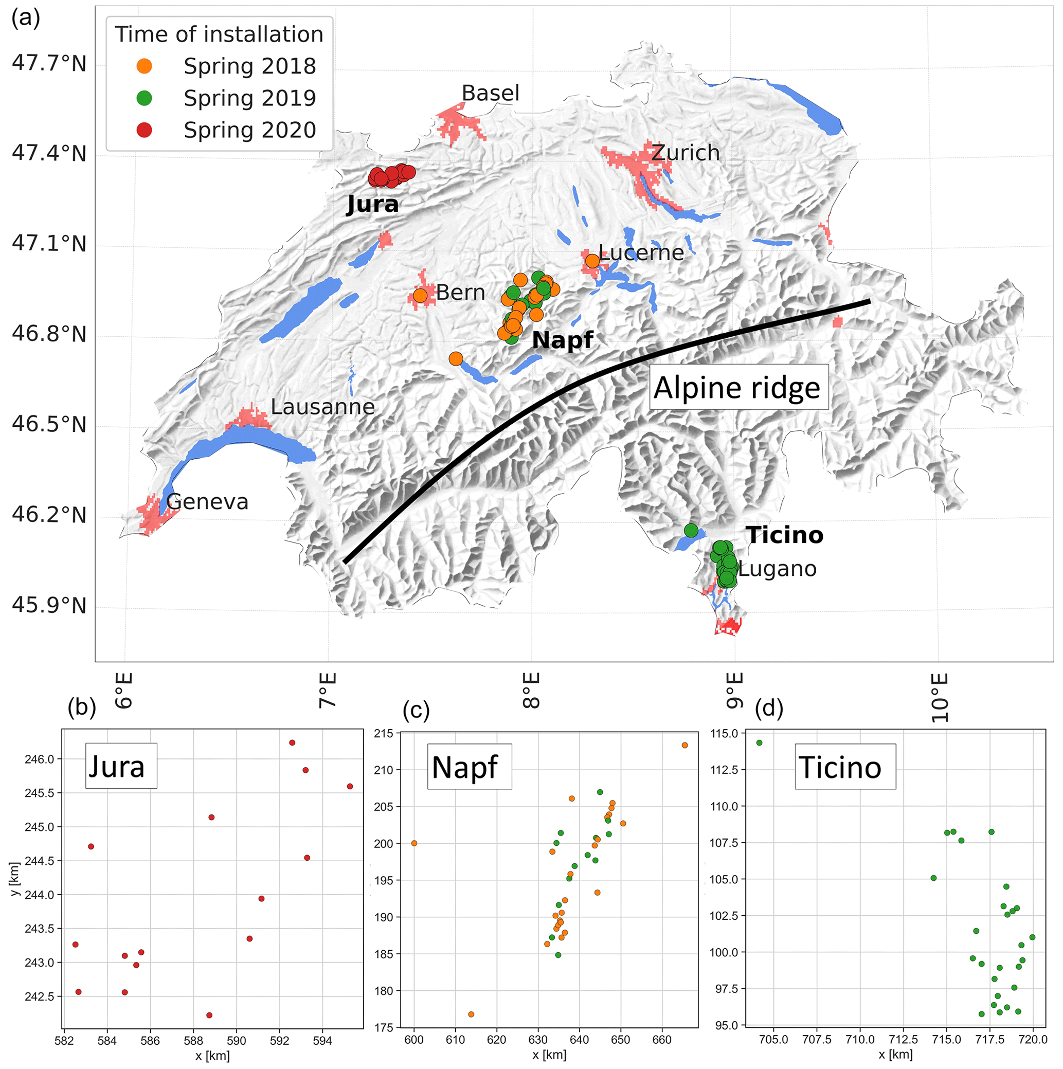
Figure 1 (a) Map of Switzerland showing the locations of the 80 sensors, according to their installation date in the three hail-prone regions (Jura is 15, Napf is 38, and Ticino is 27). Red patches show urban areas, and the black line denotes the alpine ridge. (b–d) Enlargement of the three hail-prone regions showing network density and scale in kilometres. The areas covered by the three networks are approximately 53 km² for Jura, 440 km² for Napf (excluding the three sensors in Bern, Lucerne, and Thun) and 86 km² for Ticino.

2.1.2 Measurement process

Each sensor is designed as a Makrolon thermoplastic disc, with a diameter of 50 cm (Fig. 2), providing a sensing area of approximately 0.196 m². The disc oscillates when hit by a hailstone, and a highly sensitive piezoelectric microphone records the oscillations, which are then converted to the hailstone kinetic energy (in joules) through a log-linear calibration curve.

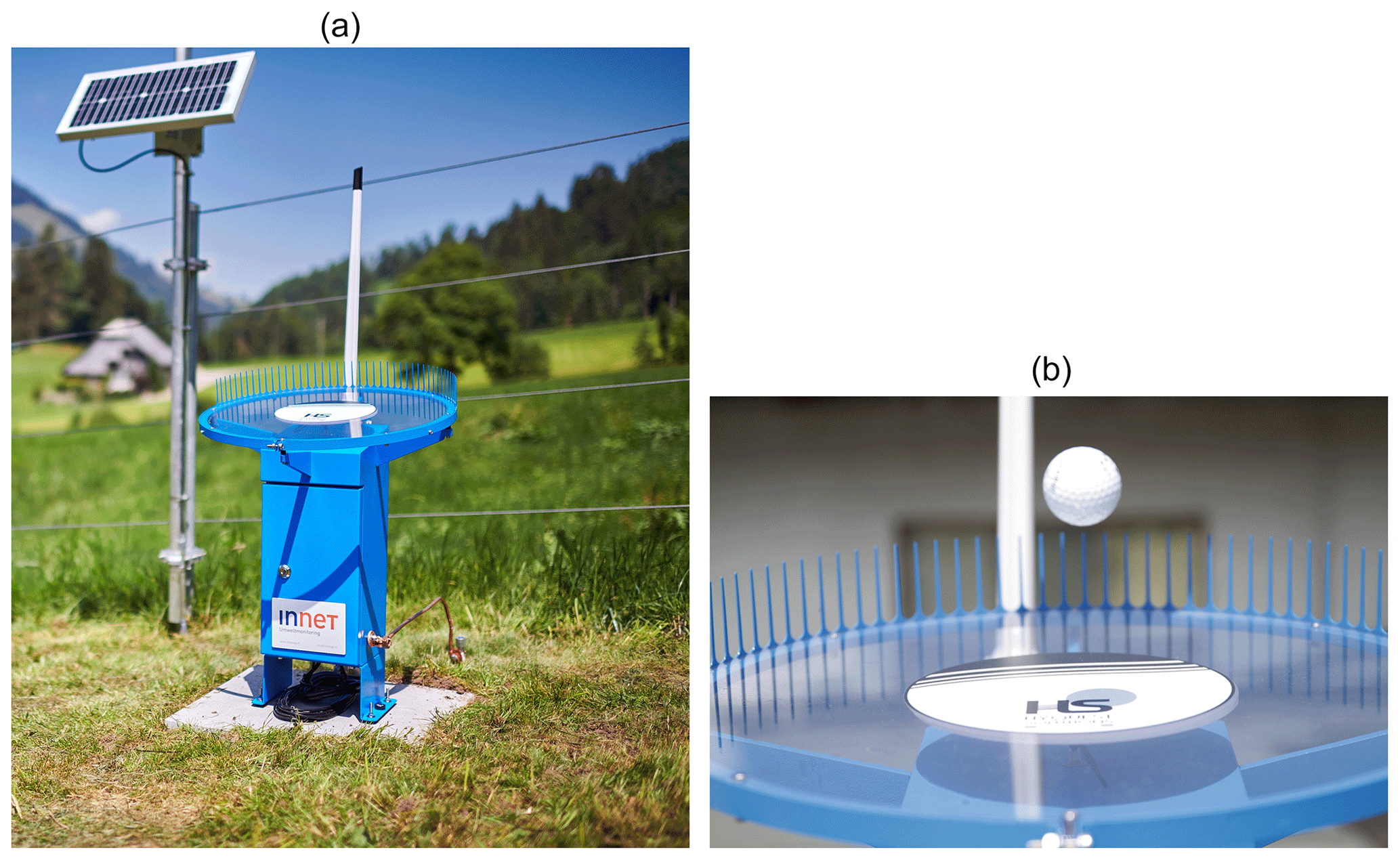
Figure 2 (a) Picture of one of the automatic hail sensors installed as part of the Swiss Hail Network project (photo credit: © Manu Friederich). (b) Enlargement of the sensor Makrolon disc as a golf ball is falling (photo credit: La Mobilière/Sascha Moetsch).

The calibration procedure (Riehle and Schön, 2021), which allows us to convert the electric signal output to an estimate of the kinetic energy, is a key step in the measurement process. Each sensor is individually calibrated by the manufacturer under laboratory conditions before its delivery (lab calibration). As each sensor is exposed to various weather conditions throughout the year, it has to be recalibrated once a year either before or at the beginning of the hail season (field calibration). The field calibration is done using a portable calibration unit that can be fixed to the sensor. Three rods of different known masses which are screwed onto a polyamide sphere at the bottom are each dropped 12 times from two fixed heights on the same calibration point. A material factor (determined at the factory using a hail gun) takes into account the different impact behaviour of ice and polyamide. The average of the signal responses is calculated for each of the six different mass–height combinations, giving six points used to fit a power law between the voltage signal and the kinetic energy. This power law is then used as the calibration curve to translate the voltage signal of hailstone impacts to a kinetic energy estimate.

2.1.3 Hailstone diameter estimation

The hailstone diameter is then determined from the kinetic energy, assuming spherical hailstones with constant drag coefficient, as follows (Pruppacher and Klett, 2010):

$$\begin{array}{}\text{(1)}& D={\left[{\displaystyle \frac{\mathrm{9}\cdot E_{\mathrm{kin}}\cdot {\mathit{\rho }}_{\mathrm{air}}\cdot c_{\mathrm{w}}}{{\mathit{\rho }}_{\mathrm{ice}}^{\mathrm{2}}\cdot \mathit{\pi }\cdot g}}\right]}^{\mathrm{0.25}},\end{array}$$

where D is the equivalent spherical hailstone diameter, E_kin is the kinetic energy of the hailstone, ρ_air=1.2 kg m⁻³ is the surrounding air density, c_w=0.5 is the drag coefficient, ρ_ice=870 kg m⁻³ is the hailstone ice density, and g=9.81 m s⁻² is gravity. Diameter calculations using Eq. (1) and the listed values for its parameters are directly implemented in the hail sensor software by the manufacturer. We note that values of ρ_air, ρ_ice, and c_w can vary, depending on the local environment and from one hailstone to another, but that similar values have been used previously in the literature (e.g. Waldvogel et al., 1978a; Brimelow, 2018; Manzato et al., 2022).

While Eq. (1) has been successfully used in the early literature (e.g. Federer and Waldvogel, 1975; Ulbrich and Atlas, 1982), the more recent literature has shown that the assumptions on which it is based are not always satisfied. First, hailstone growth results in a variety of hailstone shapes, and hailstones tend to become increasingly non-spherical with increasing size (see, for example, Shedd et al., 2021). Then, the drag coefficient of hailstones (even spherical ones – but to a lesser extent) depends on the Reynolds number, and their density can vary greatly (see, for example, Heymsfield et al., 2014, 2018, 2020).

We focus on relatively small hailstones, and most of them have an estimated diameter of less than 20 mm, such that the assumption of spherical hailstones remains a reasonable approximation (Waldvogel et al., 1978a; Shedd et al., 2021). Therefore, we do not expect the drag coefficient to significantly depart from the 0.5 value (Waldvogel et al., 1978a; Shedd et al., 2021). However, we note that, as the hail sensor primary output is the hailstone kinetic energy, relations other than Eq. (1) could be used and compared to estimate the equivalent hailstone diameter. We discuss this point further in the conclusion.

2.1.4 Known sources of uncertainties

As the sensor is continuously exposed to variable weather conditions, it is likely that its sensitivity slightly changes over the course of the year. The ambient temperature also influences the calibration process (personal communication from inNET Monitoring AG, 2022). Thus, despite the yearly field calibration, the sensitivity of the sensor to weather conditions introduces uncertainty in the kinetic energy measurements. Another source of uncertainty is the impact location on the sensor plate. The piezoelectric microphone is located under the centre of the Makrolon disc, and consequently, an impact close to the border of the disc will result in a slightly lower signal for the same hail size. The manufacturer indicates a 20 % uncertainty in the estimation of the kinetic energy and recommends that we work with hail classes of 5 mm diameter ranges, although the sensor produces measurements with a precision of several decimal places (Riehle and Schön, 2021).

2.1.5 Sensor dead time and saturation

A known and necessary limitation of the automatic hail sensor is the “dead time” (i.e. the time period following each impact during which no other hailstone can be recorded). The dead time allows the sensor to properly record an impact by avoiding interference from other hailstones hitting the sensor right after this first impact and by letting the sensor electronics perform the necessary signal treatment. The dead time of the sensor ranges from 64 ms for hailstones smaller than 10 mm to nearly 1 s for hailstones of about 35 mm (personal communication from the sensor manufacturer, 2022), which is the size range of the largest hailstone observed so far by the network. A dead time of 64 ms corresponds to 15 impacts per second on the sensor plate or 70 impacts per second per square metre. When the sensor is not able to record a new impact because it happens during the dead time of a previous impact, we call it saturation.

We investigated the influence of saturation and quantified to which extent it affects the measured hailstone density (number of hailstones per second). We used an approach from radiation detection (Lucke, 1976) to estimate the “true” detection rate R as follows:

$$\begin{array}{}\text{(2)}& R={\displaystyle \frac{N}{\left(T-{\sum }_{i=\mathrm{1}}^N{\mathit{\tau }}_i\right)}},\end{array}$$

where N is the number of recorded impacts, T is the duration of a hail event, and τ_i is the dead time of the ith hailstone. Equation (2) has been adapted to account for the hailstone size dependence of the dead time (hence the τ_i). We then multiply T by R to obtain an adjusted number of impacts, and we use this adjusted number to estimate the fraction of missed impacts.

The value of T (and subsequently R) depends on how we characterize and define a hail event (see Sect. 2.2 and 2.2.1 for details). At this stage, it is sufficient to say that the definition depends on one parameter, called the maximum blank time or t_mb, and that the estimated fraction of missed impacts, averaged over all hail events, takes values between 4 % and 4.6 % for the considered values of t_mb. Hence, the average fraction of the missed impacts remains low when compared to all impacts. The fraction can be higher for individual events (up to 10 %), especially for those events with a higher hit rate (hailstones per second). We also note that we cannot know the diameters of the missed hailstones.

Finally, hailpads can also become saturated (Manzato et al., 2022). Saturation on hailpads can happen when their surface is covered in dents (impacts) made by numerous hailstones, such that subsequent hailstones can fall inside those existing dents and cannot be distinguished. For a more in-depth discussion about hailpad saturation, we refer the interested reader to Manzato et al. (2022).

2.1.6 Minimum signal threshold

A minimum signal threshold is set by the manufacturer after lab calibration to avoid recording the impacts of large raindrops or graupel, whose kinetic energies could approach those of small hailstones (Pruppacher and Klett, 2010). This threshold is initially set to correspond to a 5 mm diameter hailstone, which is consistent with the World Meteorological Organization (WMO) definition of hail (which is the precipitation of ice particles with a diameter larger than 5 mm; World Meterological Association, 2017).

However, a close examination of the sensor data revealed that this threshold had not been adjusted after the field calibrations. Consequently, it happened that in some cases the threshold no longer exactly corresponded to a 5 mm hailstone but to a larger or smaller diameter, according to the new field calibration.

In the case of a less than 5 mm threshold, this led to the recording of graupel or possibly large raindrops. For such cases, a simple filtering of all impacts with an estimated diameter lower than 5 mm can correct the data.

In the case of a more than 5 mm threshold, some small hailstones larger than 5 mm might not have been recorded properly. This is more problematic, as the exact number of missed hailstones due to this higher threshold cannot be estimated.

It was not feasible to calculate the number of cases for which the threshold departed significantly from 5 mm from the archived calibration records. Considering the daily records by sensor, an examination of the data revealed that in 37 cases among 1447 (2.5 %), hailstones of less than 4 mm have been recorded. We cannot make the same estimation for a threshold larger than 5 mm as it is not possible to say if this was indeed due to the threshold or because the hailstones were all larger. A reasonable assumption would be that cases in which the threshold was significantly larger than 5 mm happened on average as often as cases where it was significantly smaller, leading to 2.5 % of cases in which the threshold prevented the measurements of hailstones smaller than 6 mm. Although we have to bear in mind that in some cases the lower end of the hail size distribution had been truncated due to this larger than 5 mm threshold, we believe that a 2.5 % missing rate is acceptable. We note that from the 2023 hail season onward, the signal threshold will be adjusted after each field calibration, such that the lower bound of diameters is fixed to 5 mm for all sensors and at all times.

2.1.7 Radar reflectivity filter

Not only hydrometeors can generate impacts on the sensor; examples include animals, such as birds, goats, cats, and dogs, touching the sensor or flying objects in case of strong winds, such as small branches or light gravel. For this reason, we use a radar reflectivity filter to ensure that there is a storm environment in close to the vicinity of the sensor. For that reason, we demand that the maximum reflectivity within a radius of 4 km around the sensor at the time that the sensor is hit is equal to or higher than 35 dBZ. This reflectivity threshold is operationally used in the thunderstorms radar tracking (TRT) algorithm by MeteoSwiss to identify storm objects (Hering et al., 2004; Nisi et al., 2016, 2018) and was used in Barras et al. (2019) to filter hail crowdsourced reports. While hail is usually associated with higher maximum reflectivity in radar-based hail algorithms (e.g. 40 to 50 dBZ; Waldvogel et al., 1979; Witt et al., 1998; Joe et al., 2004), Barras et al. (2019) found that it might be too restrictive. The 4 km radius accounts for the wind drift of hailstones Barras et al. (2019). This filter removed 1785 hailstone impacts out of 14 085 from our dataset.

2.2 Examples of measurements and event delineation

An interesting feature of the automatic hail sensors is that it provides the precise timing of each hailstone impact. This time information can be used to define the local duration of a hail event, just by looking at the first and last hailstones that hit the sensor and defining those times as the beginning and end of the event. However, it is sometimes not possible to unambiguously define the beginning and end of an event.

To illustrate this, we show five examples of impact time series (Fig. 3). The event can be clearly identified in Fig. 3a. Almost 300 impacts are registered within 3 min, with a clear start and end. The time series in Fig. 3b shows two impact clusters separated by 15 min, followed by two other impacts 45 min later. It is not straightforward to say whether the two first impact clusters come from the same hailstreak or from two distinct ones, due to the variability in the hailstreak dimensions and storm velocities. Based on studies from various countries, Brimelow (2018) found that the majority of hailstreaks are less than 5 km wide, increasing to 10 to 15 km for more organized hailstorms, with maximum widths ranging from 25 to 30 km. Nisi et al. (2018) analysed a 15-year radar-based climatology of hailstreaks from Switzerland and found average streak lengths from 10.4 to 36.2 km and an average streak duration from 25 to 60 min. This gives an average storm speed from 25 to 33 km h⁻¹. Trefalt et al. (2018) analysed a severe hailstorm in Switzerland and found that the storm mean velocity was approximately 6 km h⁻¹. They also found that other severe storms had speeds ranging from 4.5 to 18.6 km h⁻¹. Using an object-based analysis of the simulated thunderstorms in Switzerland, Raupach et al. (2021) found storm velocities ranging from a few kilometres per hour to 40 km h⁻¹. Combining those estimates of hailstreak areas and storm velocities, we conclude that the same storm can produce hail in the same place for durations ranging from a few minutes to just over an hour. This does not mean that hailstones would be produced continuously but that two or more series of hailstones separated by several minutes without hail (a blank period) could potentially be produced by the same storm at the same place.

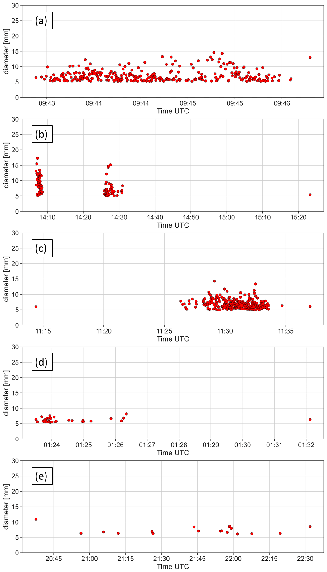
Figure 3 Time series of hailstone impacts; the y axis shows the estimated diameter (mm). Note the different timescales on the x axis. (a) 8 July 2021 at Trafohaus, Bironico. (b) 24 July 2021 at Mösli, Marbach. (c) 26 July 2021 at Bergstation Marbachegg. (d) 2 August 2019 at Onecars, Lugano. (e) 6 August 2021 at Scuola Elementare Cadro.

Figure 3c, d, and e present other examples of situations in which hailstone impacts are separated by blank periods. Figure 3e is particularly striking, as only 18 impacts are registered in nearly 2 h. One might ask whether those impacts really correspond to hail. The average maximum reflectivity during the impacts is 47 dBZ, and several neighbouring sensors also recorded impacts during the same time period with the same scarce pattern, indicating that hail was indeed responsible for the impacts. A more detailed analysis using radar data, numerical model data, and crowdsourced observations would be needed to understand the storm patterns and attribute the impacts to distinct hailstreaks. As we cannot investigate all of the time series of the impacts in such detail, we need a simple conceptual model to group hailstone impacts into distinct events to further analyse the hail duration.

2.2.1 Methodology for defining a hail event

We define a hail event as a series of consecutive impacts recorded by an individual sensor separated by less than t_mb in time. If two impacts are separated in time by more than t_mb, then they belong to two different events. The choice of t_mb determines the number of events and their duration. Large values of t_mb will merge events, thereby decreasing the number of events and increasing their average duration. As an example, the time series of Fig. 3e is considered to be a unique event for t_mb=20 min, while it is split into six distinct events for t_mb=10 min, including three events with a single impact, one with two impacts, one with three impacts, and another with 10 impacts.

We systematically considered values of t_mb, ranging from 1 min to 2 h, and found that when t_mb increases from 20 to 30 min then there is a jump in the increase in the average event duration (not shown). This suggests that we are grouping together events which are separated by a longer period without hail. Blank periods of 30 min or more would imply both particularly large and slow-moving storms. We also found that values of t_mb of less than 5 min are too small and lead to an artificially high number of events with a few impacts. However, as the choice of t_mb can impact the subsequent analysis of the local hailfall duration, we decided to investigate t_mb values of 5, 10, 15, and 20 min more closely and present a sensitivity analysis in Sect. 3.

The identification of hail events could be done using a temporal kernel density estimate or a clustering algorithm. However, we note that the variability in the hailstone temporal density between events and the limited number of impacts in some events could represent a challenge in the use of such methods.

2.3 Hailpad data

The closest measurement device to an automatic hail sensor is a hailpad; they measure hail at ground level and on a surface level of similar scale. Hailpads have an area of about 0.291×0.395 m =0.115 m², which is half of the sensor area (0.196 m²). Consequently, it makes sense to compare their observations.

Contrary to some of its neighbouring countries, Switzerland does not have an operating network of hailpads. A network of around 300 hailpads was set up during the Grossversuch IV experiment (Federer et al., 1986), which took place from 1977 to 1981. Several studies presented results and hailstone size distributions using Grossversuch IV hailpad observations (e.g. Waldvogel et al., 1978b, a; Mezeix and Chassany, 1983; Federer et al., 1986; Smith and Waldvogel, 1989; Schmid et al., 1992). However, each of these studies uses a different subset of Grossversuch IV hailpad measurements. Then, they provide only averaged quantities and give limited details on the hailpad selection process (e.g. is there a minimum number of dents needed to consider a hailpad? What is the calibration fit?), precluding a precise comparison with the hail sensor observations. The same conclusions were reached when reviewing hailpad studies covering other regions of the world (Fraile et al., 2003; Sánchez et al., 2009; Pocakal, 2011; Eccel et al., 2012).

For those reasons, we chose to work with hailpad observations from a station network of northeastern Italy, which was collected during the 1988–2016 (29 years) warm seasons (Manzato et al., 2022), because direct access to both the detailed dataset and to someone with in-depth knowledge about it was possible. While the observations were made in two different countries, Switzerland and northeastern Italy are geographically close (approx. 300 km apart), at the same latitudes, are close to the Alpine chain, and hence subject to similar synoptical-scale weather systems (Giaiotti et al., 2003). Therefore, we do not expect the hail size distributions to differ substantially on average. Moreover, both datasets include multiple hailstorms from several years, contributing to averaging out the effects of storm environments (Cheng et al., 1985).

The selection criteria applied to the hailpads were to keep only valid dents corresponding to hailstones of at least 6 mm with an aspect ratio (major $/$ minor axis) between 1 and 2. The reason was that dents corresponding to small diameters and very high aspect ratios likely do not represent true hailstone signatures. All hailpads with at least one valid impact were retained. This corresponds to 7782 hailpads, totalling 747 759 valid impacts. For details on the processing of hailpads and the selection criteria, the interested reader is referred to Manzato et al. (2022).

The hailpads are usually collected and replaced by volunteers after each hailstorm. It is likely that the volunteer will wait for the storm activity to end before going outside to collect the hailpad. We also note that cases in which the same station collected more than one hailpad on the same day are extremely rare, such that we can consider that each collected hailpad contains a daily aggregation of hail dents. Consequently, we also make daily aggregations of the impacts recorded by a given sensor and consider only impacts with estimated diameters of at least 6 mm to compare our data with the hailpad data in Sect. 3.2.1. With these selection criteria, our sample is composed of 8958 hailstones and 1058 daily aggregations.

3 Results and discussion

3.1 General observations, hailstone size, and kinetic energy distributions

From July 2018 (when the first sensors were installed) to August 2022, 12 300 hailstone impacts were registered (Fig. 4). Few impacts were recorded in 2018 and 2019, as the sensor network was not yet fully deployed. The highest number of yearly impacts (6400) was recorded in summer 2021, during a particularly active hail season (Kopp et al., 2022). The largest daily number of impacts for an event is 405 and has been recorded by the sensor of the Bergstation in Marbach (Napf region) on 26 July 2021 (see Fig. 3c).

Figure 4 Monthly number of impacts (all sensors).

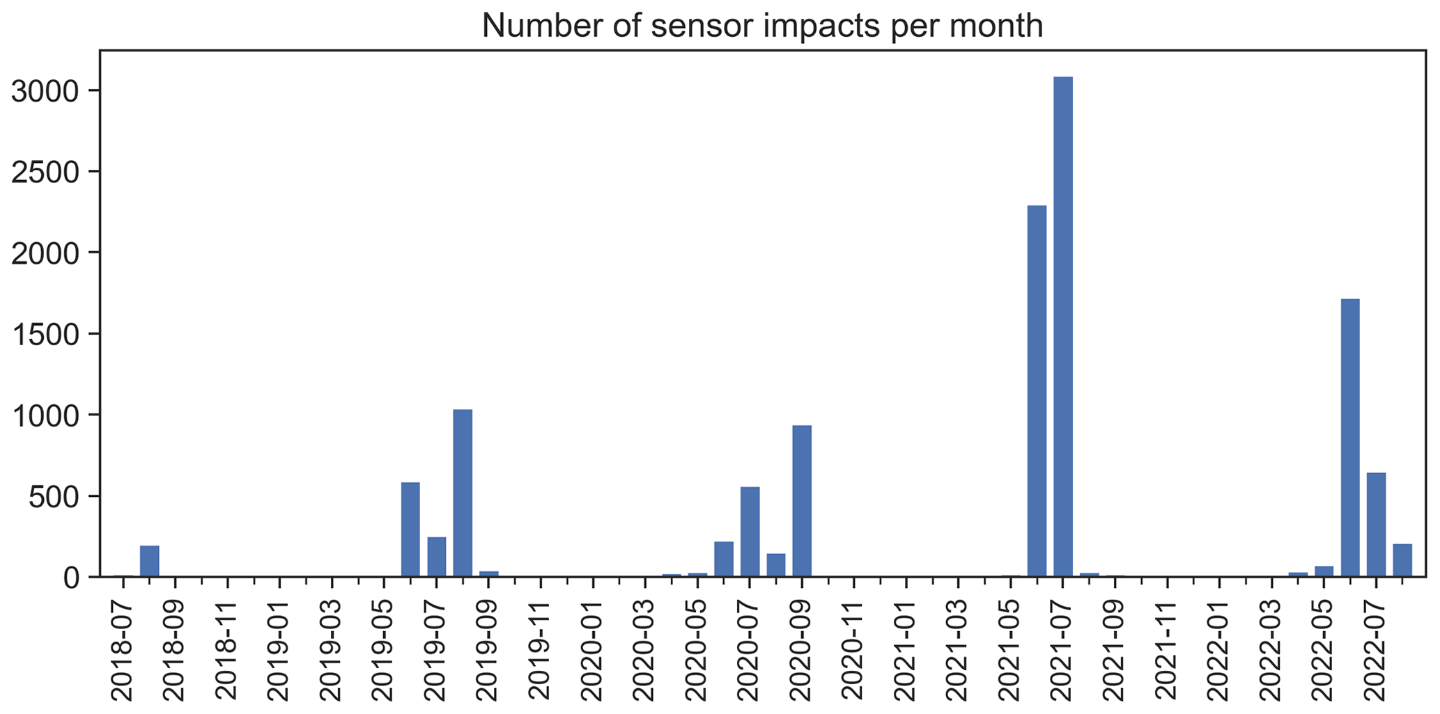
Figure 5a shows the hailstone diameter probability distribution and Fig. 5b the kinetic energy distributions. The largest hailstone had an estimated diameter of 33 mm, which corresponds to a kinetic energy of 5.2 J. The median diameter is 6.7 mm, and the median kinetic energy is $\mathrm{9}\times {\mathrm{10}}^{-\mathrm{3}}$ J. Only 41 impacts (0.33 %) had an estimated diameter of 20 mm or more. An exponential fit (red line in Fig. 5a) of the hailstone probability distribution gives the following (with D in mm):

$$\begin{array}{}\text{(3)}& P\left(D\right)=\mathrm{2.48}(\pm \mathrm{0.42})\times {\mathrm{10}}^{-\mathrm{0.16}(\pm \mathrm{0.01})D}.\end{array}$$

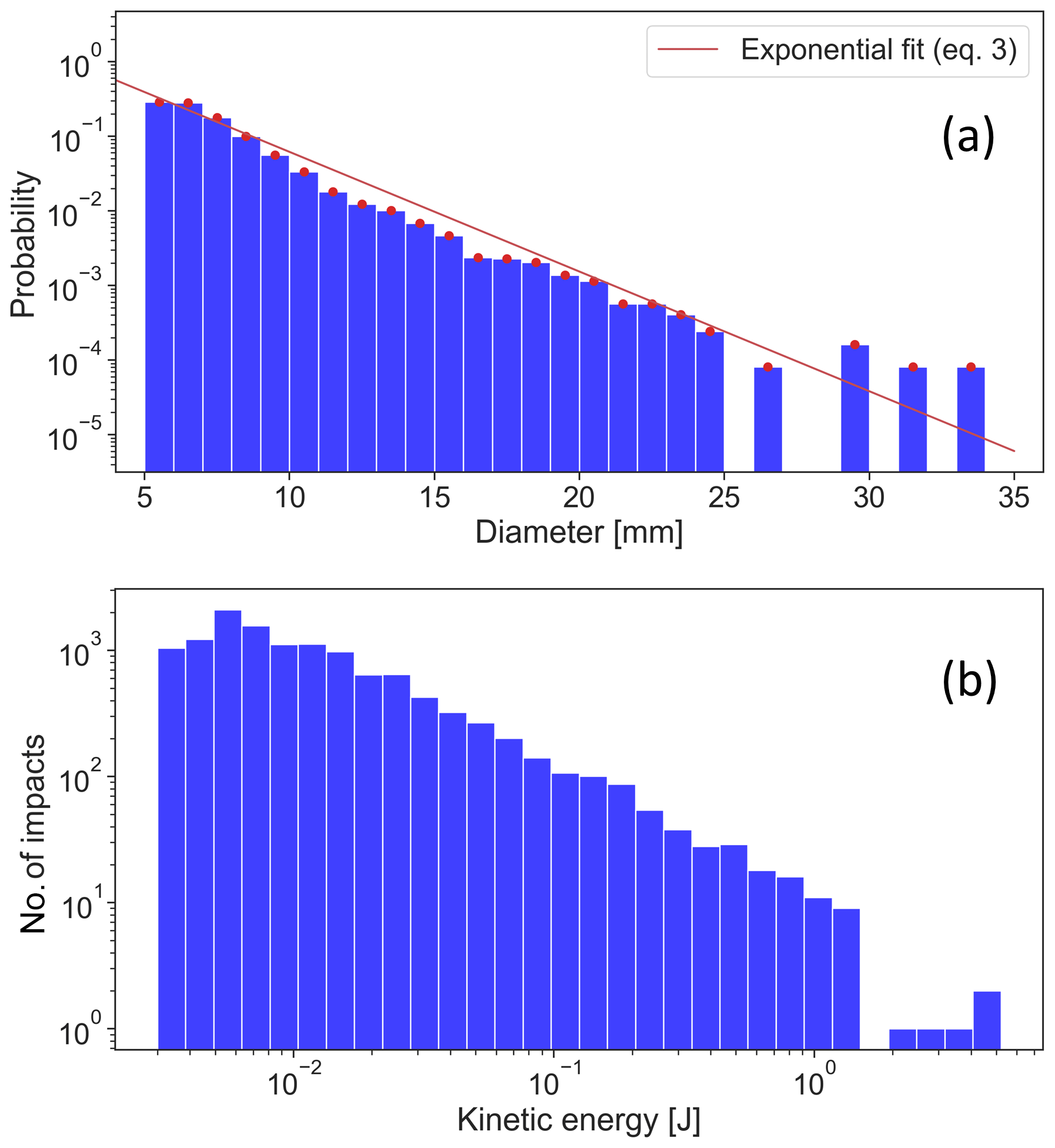
Figure 5 (a) Hailstone diameter probability distribution in 1 mm size classes (12 300 hailstones with diameter >5 mm), with an exponential fit (red line). (b) Hailstone kinetic energy distribution; note that the x log scale is the same sample as in panel (a).

The fit works reasonably well for diameters up to 25 mm but underestimates the largest hailstone probabilities.

3.2 Comparison with hailpad data

We first compare the distribution of the number of hailstones per hail sensor and hailpad. Then we look at the averaged hail size distribution (HSD) at the ground level by merging all measurements for each device.

3.2.1 Hail sensor and hailpad distributions

Figure 6 shows the probability distribution of the number of hailstones per hailpad and hail sensor. The two distributions differ substantially. There are proportionally many more sensors than hailpads with a few (one to five) hailstones and fewer sensors than hailpads with more than five hailstones.

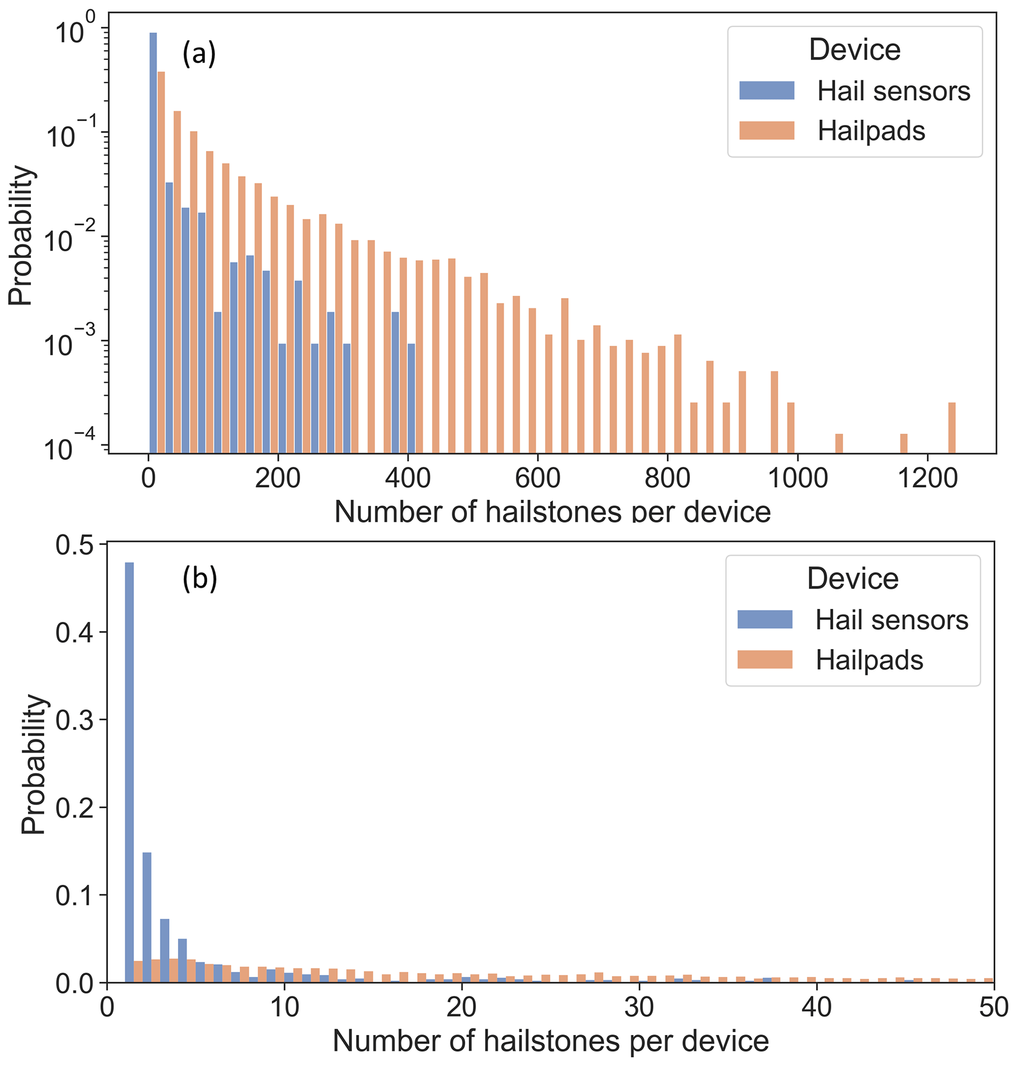
Figure 6 (a) Probability distributions (logarithmic y scale) of the number of hailstones per hail sensor (orange) and hailpad (blue). (b) The same distributions as in panel (a), with a linear y scale and a focus on hailstone numbers from 1 to 50.

The difference in the distributions for large hailstone counts can be explained by the limited sample size of the sensors compared to the hailpads. Hence, the tail of the distribution for hail sensors is probably missing the large hailstone counts. Indeed, the largest number of hailstones registered by a hailpad from Manzato et al. (2022) is 1244, and 362 hailpads recorded a higher hailstone number than the largest number recorded by a sensor (405 hailstones).

Despite our smaller sample size, there are 507 sensors and only 193 hailpads with a single hailstone. A plausible explanation is that more than one hailfall is overlaid on the same hailpad. This could happen because the volunteers checking hailpads with a low number of dents (possibly of a small size) might not notice them and would leave the hailpad exposed instead of replacing it with a new one. Volunteers could also not notice hailfalls with very low hailstone densities and thus not check the hailpad at all. This would lead to a lower relative number of hailpads with a few hailstones and a higher relative number of hailpads with many hailstones. It might also be that, despite the radar reflectivity filter, some impacts registered by the sensor were not caused by hailstones. A few exceptionally large raindrops or small windblown objects could have generated those one to five impacts.

As stated in Sect. 2.3, the area covered by a hailpad and a hail sensor are not the same. We looked at the distributions of the areal densities (impacts per m²) by normalizing both devices by their respective size. The same differences were noted in the distributions of the areal densities as in Fig. 6 (not shown).

3.2.2 Hailstone size distributions

The hailstone size distributions (HSDs) observed at the ground level by the hail sensors and the hailpads are compared in Fig. 7. A visual inspection of the curves reveals that they are very similar for diameters up to 18 mm, with a slight difference for the smallest diameters. The distributions start to differ for diameters larger than 18 mm (Fig. 7a). However, there is only a limited number of data points in the hail sensor sample for those diameters, which explains the discontinuities of the distribution. Using a fit of the form $a\times {\mathrm{10}}^{-bD}$, similar to Eq. (7) in Manzato et al. (2022), we found the following:

$$\begin{array}{}\text{(4)}& {\displaystyle }P\left(D\right)=\mathrm{4.84}\times {\mathrm{10}}^{-\mathrm{0.22}D}\text{for hail sensors}\text{(5)}& {\displaystyle }P\left(D\right)=\mathrm{4.44}\times {\mathrm{10}}^{-\mathrm{0.21}D}\text{for hailpads},\end{array}$$

which works reasonably well for diameters up to 18 mm but underestimates the largest hailstone probabilities.

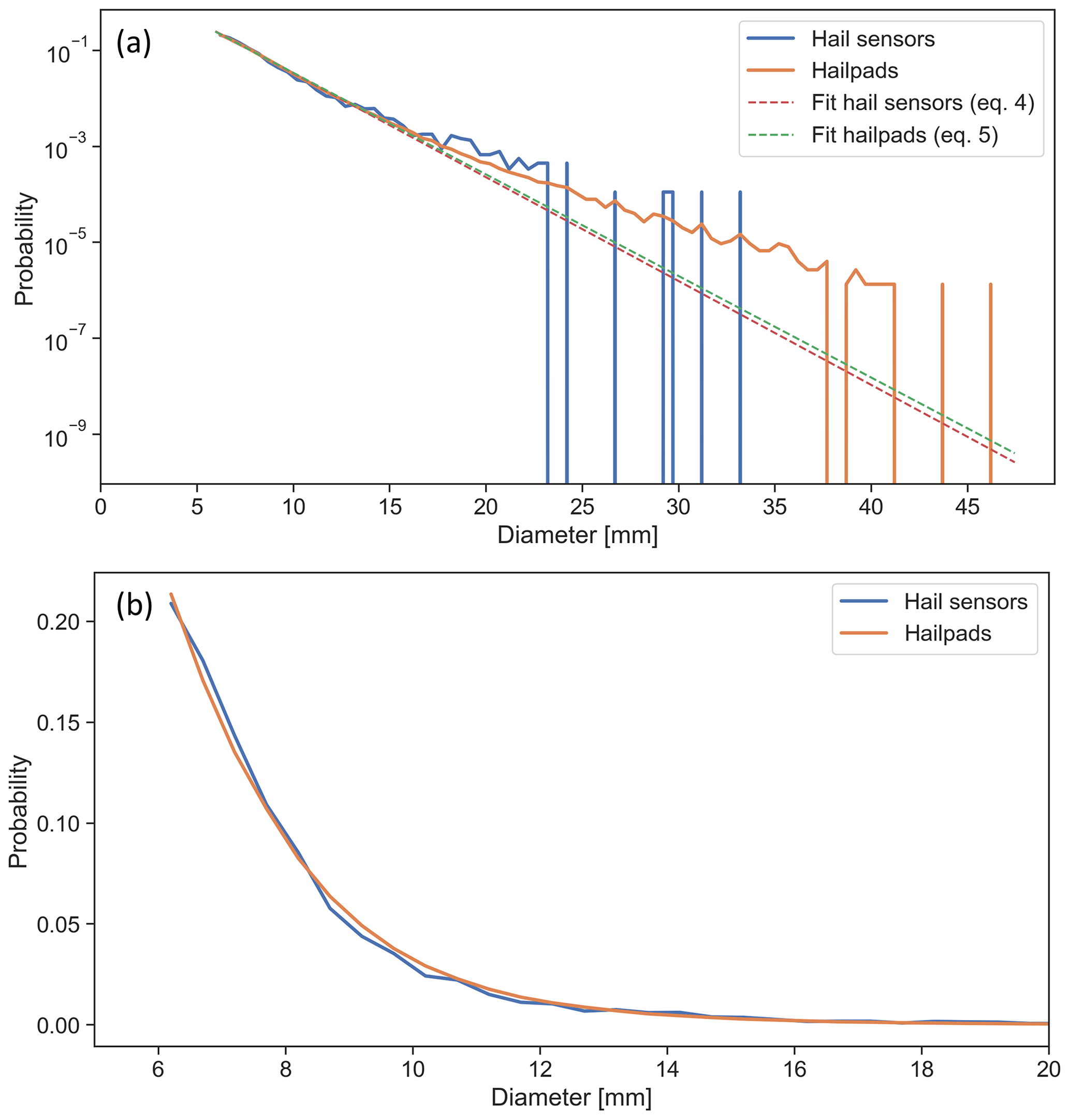
Figure 7 (a) Hailstone size distribution (probability) from hail sensors (orange) and hailpads (blue). The data are binned from 6 to 47 mm, using bins of 0.5 mm size (i.e. the first bin groups the diameters from 6 to 6.5 mm). (b) The same distributions as in panel (a) but with a linear y scale and a focus on diameters from 6 to 20 mm.

We looked at various statistical tests to assess the similarity of the hail size distributions from hail sensors and hailpads. Figure 8 shows a quantile–quantile plot (Q−Q plot) of the two distributions. Each dot represents a percentile, and we see that all dots except the last one are on, or very close to, the red line, showing the similarity of the distributions up to the 99th percentile. The difference in the maximum diameter of the distributions (33 mm for hail sensors; 46 mm for hailpads) explains the large difference in the 100th percentile. A Kolmogorov–Smirnov test (statistic =0.03; p value =1) did not reject the null hypothesis that distributions are similar. A standardized mean difference of $\mathrm{4.6672}\times {\mathrm{10}}^{-\mathrm{3}}$ showed that the means of the distributions are comparable. A more stringent chi-squared test on all of the percentiles of the distributions rejected the null hypothesis that the distributions are the same (statistic =149.95; p value =0.0007). However, the null hypothesis was not rejected at a 5 % confidence level when considering the first 95 percentiles of the distributions in the chi-squared test (statistic =113.44; p value =0.0840). Based on those tests, we conclude that the hail size distributions (HSDs) are very similar, except for the tail.

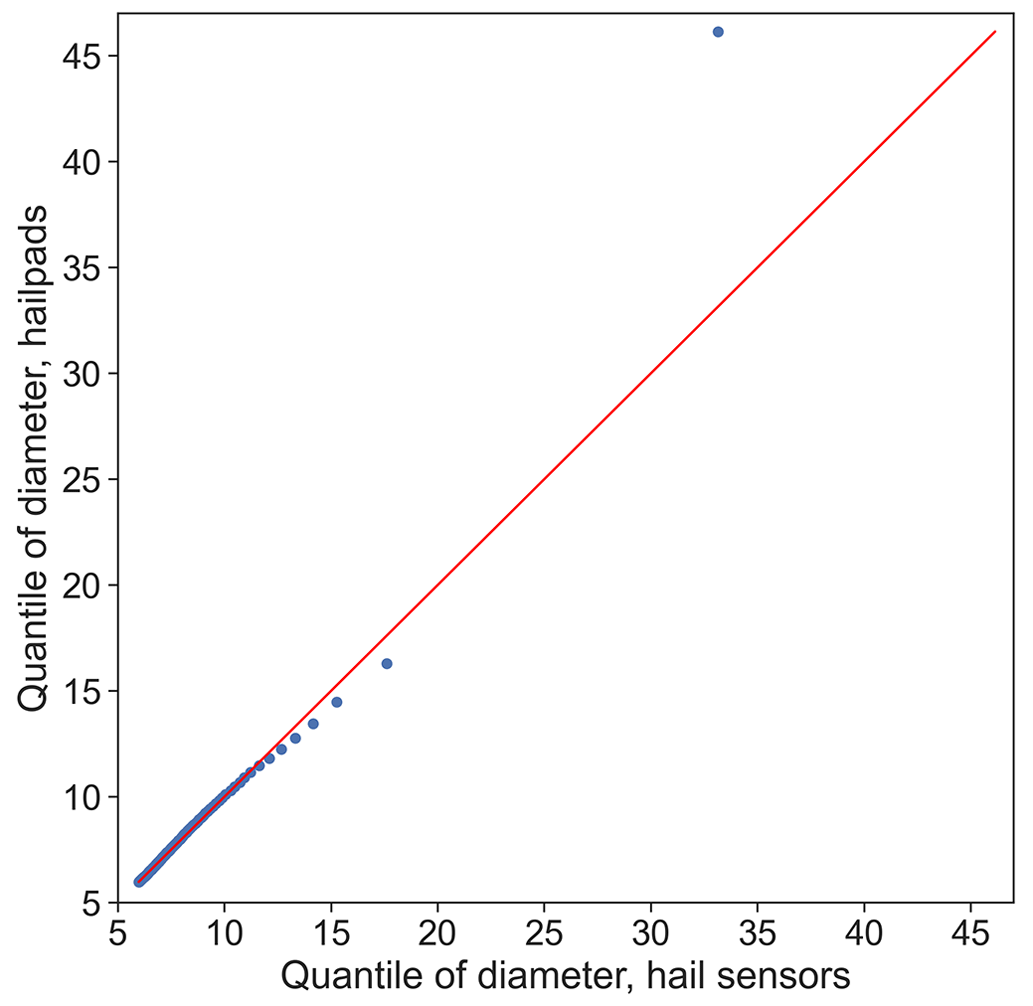
Figure 8 Quantile–quantile plot of the hail size distributions for hail sensors (x axis) and hailpads (y axis). Each 1 % is shown.

The similarity of the HSDs is particularly interesting when considering the observations in the previous section. First, it shows that, despite the fact that the distributions of the number of hailstones per hail sensor and hailpad are different, their overall hailstone size distributions are almost identical. Second, it shows that the two devices give coherent results when several events are pooled. We cannot draw any further conclusion, as the hail sensor and hailpad observations were not made on the same hailstorms. Moreover, they were made in different regions and in different years. It would also be interesting to redo this comparison, when the sample size from hail sensors becomes larger, to see if the difference in the tails remains.

We remark here that, due to their limited area, hailpads and hail sensors cannot capture the entire hail size distribution of a hailstreak. Aerial drone photography can offer promising perspectives in that sense (see, for example, Soderholm et al., 2020; Lainer et al., 2023), provided that one is lucky enough to have a drone ready and available in the right place at the right time.

3.3 Analysis of time-related quantities

We use the time information provided by the sensor to investigate the local hailfall duration, the time distribution of hailstones during an event, the hit rate (number of hailstones per second), and the relative time when the largest hailstone of an event is measured.

3.3.1 Hail event duration and sensitivity analysis

We investigate hail event duration and its sensitivity to the parameter t_mb used to delineate the events (t_mb values of 5, 10, 15, and 20 min). Furthermore, we stratify the hail events by the number of impacts in three categories, namely 2 to 5 impacts (scarce), 6 to 25 impacts (intermediate), and >25 impacts (dense). One reason for doing this is that events with very few impacts can artificially decrease the average duration, as they are usually shorter than events with a larger number of impacts. The value of 25 impacts to define dense events was chosen to have a sample large enough (around 100 events). We introduced an intermediate category (6 to 25 impacts) to clearly separate scarce events from dense hail events. Single-impact events are not considered because their duration cannot be properly defined. From the initial 12 300 impacts, approximately 1000 events with a single impact have been removed from the sample.

We see that the number of events and impacts in each category (first two columns in Table 1) almost do not change when varying t_mb, which means that the size of the samples remain constant and is comparable.

Table 1 Event statistics for different (t_mb) values stratified by impact numbers. From left to right are the number of events and hailstone impacts and the mean value, the first quartile, the median value, the third quartile, and the maximum value of event duration in seconds. The first quartile, median value, and third quartile of the cumulative time distribution of impacts (CTDIs) are given in seconds.

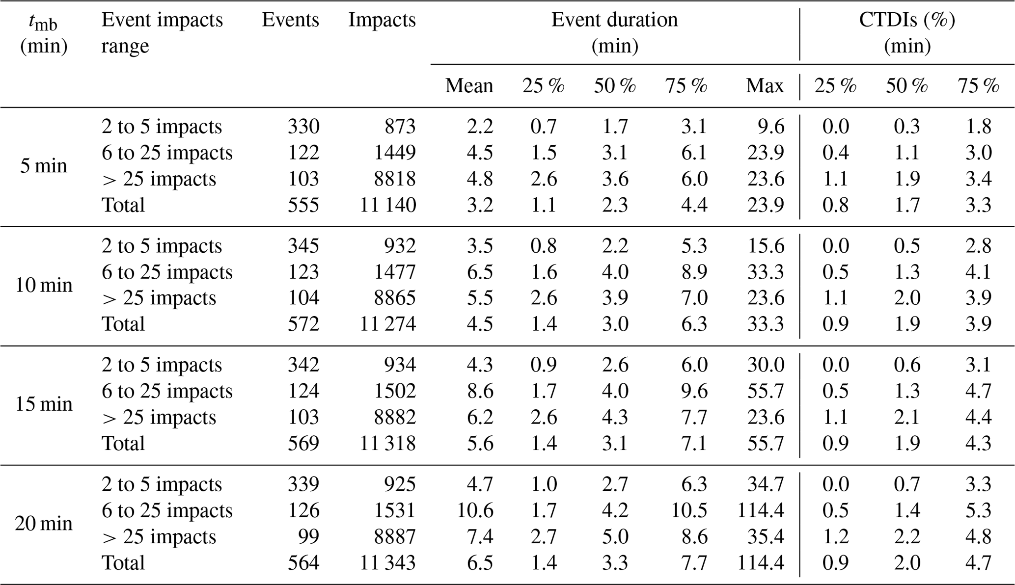
Increasing t_mb leads to a shift in the event duration distribution towards higher values (see Fig. 9 and Table 1, especially the columns with event duration statistics). Considering all events (see the rows labelled “Total” in Table 1), 50 % of the events last less than 2.3 min for t_mb=5 min and less than 3.3 min for t_mb=20 min, corresponding to a 40 % increase in median duration. In total, 75 % of the events last less than 4.4 min for t_mb=5 min and less than 7.7 min for t_mb=20 min, corresponding to a 75 % increase in third quartile duration. When considering only dense hail events (>25 impacts), 50 % of dense hail events last less than 3.6 min for t_mb=5 min and less than 5.0 min for t_mb=20 min, representing a 40 % increase in median duration. In total, 75 % of the dense hail events last less than 6.0 min for t_mb=5 min and less than 8.6 min for t_mb=20 min, representing a 44 % increase in third quartile duration. Dense hail events last longer than scarce hail events. However, quite interestingly, events in the intermediate category (6 to 25 impacts) can last longer than dense hail events, so the third quartile values (75 %) are always higher for the intermediate category.

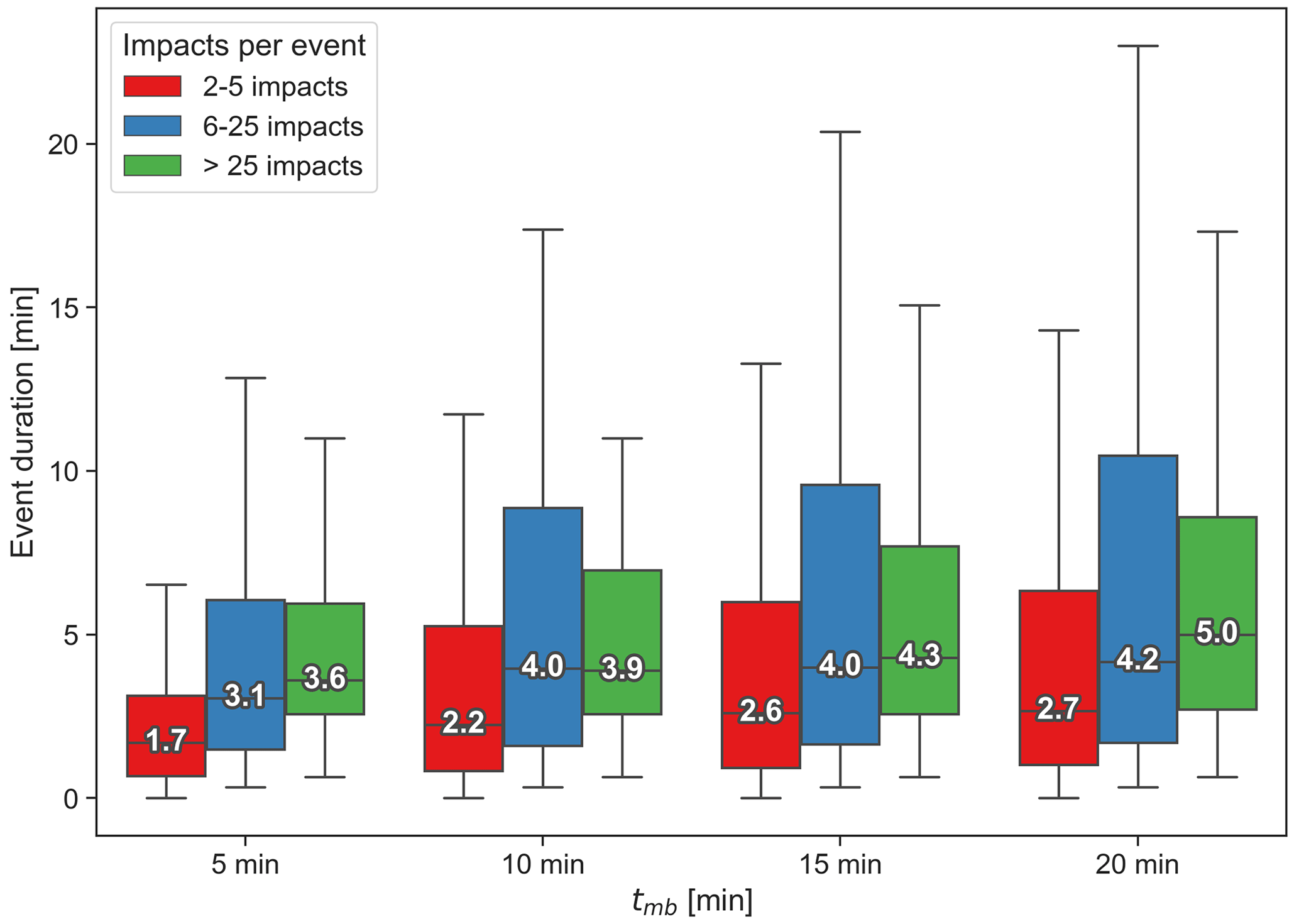
Figure 9 Box plots of the event duration for t_mb values of 5, 10, 15, and 20 min that are each stratified by the impact numbers (colours). The number shows the median duration in minutes.

We now compare our results with the existing literature. Most estimates of hailfall duration were made by human observers, with the exception of Changnon (1970) and Federer and Waldvogel (1975). Changnon (1970) found an average duration of 3.1 min for 786 hailfalls recorded in central Illinois (USA) from 1967 to 1968 with a rain gauge–hailpad network. Our average durations, considering all events (Table 1; fifth column), range from 3.2 min for t_mb=5 to 6.5 min for t_mb=20 min. Those average durations increase to 4.8 min for t_mb=5 min and 7.4 min for t_mb=20 min when considering only dense events. The short durations observed by Changnon (1970) compared to ours could be explained by the relatively high average storm speeds of around 50 km h⁻¹ that they recorded, which is significantly higher that the values observed in Switzerland (see Sect. 2.2.1). Wojtiw (1975) found an average duration of 10.1 min for 455 hailstreaks recorded in central Alberta (Canada) from 1957 to 1973 by human observers. Their study focused on major hailstreaks, from which at least 10 hail reports were obtained, with large (walnut size) hail reported at some point, which might explain the longer duration.

Počakal et al. (2009) found an average duration of 4.1 min from 11 500 reports on the occurrence of hail collected at hail suppression stations in Croatia between 1981 and 2008 by human observers. This value falls within the range of our average values. Počakal et al. (2009) mentioned that the local orography can cause a decrease in the storm speed, thereby potentially increasing the local hailfall duration. Nađ et al. (2021) discuss hail events observed in Serbia between 1981 to 2015 by human observers at hail suppression stations. They found that hailfall lasted less than 5 min in about 75 % of events, which is lower than our estimates, except in the case of scarce hail events for t_mb=5 min (3.1 min). They also found that only 8 % of events lasted more than 10 min, while in our case it ranges from 3.3 % (for t_mb=5 min) to 18.6 % (for t_mb=20 min). To our knowledge, the study of Federer and Waldvogel (1975) is the only one to have explicitly measured the local hailfall duration in Switzerland for a single hailstorm on 6 July 1973 in the Napf region. Using a hailstone spectrometer, they measured a duration of 13.5 min for an average storm speed of 6 km h⁻¹, which is very slow compared to the average storm speed in Switzerland (25 to 33 km h⁻¹; Nisi et al., 2018).

Our estimates of local hailfall duration in Switzerland are generally longer than the durations observed in other countries by previous studies. The storm velocity, which is influenced by orography, seems to be a key factor to be further investigated. The fact that an automatic hail sensor records every single hailstone impact is another important factor. The event duration is sensitive to isolated impacts recorded by the sensors that can be missed or deemed to not be part of the bulk of a hail event by human observers (see Sect. 3.2.1). For this reason, we looked at another relevant quantity, namely the cumulative time distribution of impacts during an event.

3.3.2 Cumulative time distribution of hailstone impacts

The cumulative time distribution of impacts (CTDIs) during an event indicate the proportion of the impacts recorded before a certain duration. It is similar to a cumulative distribution function in terms of the probabilities. The last three columns of Table 1 contain the first quartile, median, and third quartile values of the consolidated CTDIs, while Fig. 10 shows the entire CTDIs for the four values of (t_mb), stratified by impact number categories.

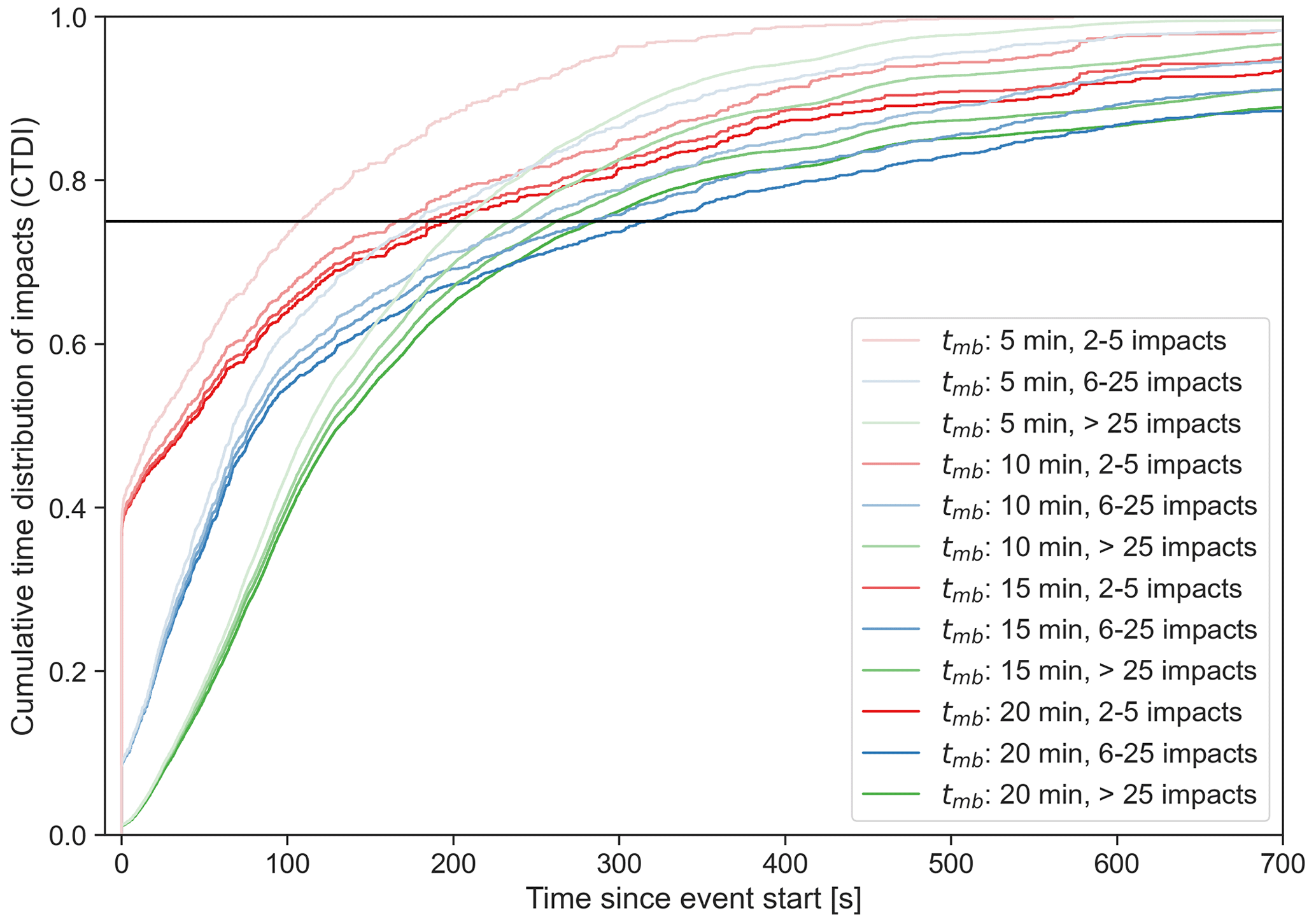
Figure 10 Cumulative time distribution of impacts for t_mb, ranging from 5 min (light colour) to 20 min (dark colour) and stratified by the event hit range (coloured curves). The horizontal black line denotes 75 % of the impacts.

We see that the third quartile of the CTDIs, when 75 % of the impacts have been recorded (black line in Fig. 10), is reached between 3.3 min (for t_mb=5 min) and 4.7 min (for t_mb=20 min). In the previous section, we found that 75 % of events last less than 4.4 min for t_mb=5 min and less than 7.7 min for t_mb=20 min. This means that the majority of the impacts occurs in a shorter time than the corresponding fraction of events and that the majority of impacts is on average concentrated at the beginning of an event.

This is interesting because hail sensors record hailstreaks at all stages of their lifecycle (initiation, maturity, and dissipation) and at all relative positions (border or centre of the streak). Considering several hailstreak records, we expected the CTDIs to increase steadily at an approximately constant rate, reflecting the average of the different lifecycle stages and relative positions of all hailstreaks. However, our results show that the CTDIs increase more rapidly at the beginning of an event than towards the end. Another way of saying it is to say that the hailstone density (hailstones per m²) is on average higher at the beginning of an event than towards the end. As a hypothesis to explain this pattern, we suggest that hailstreaks are composed of a short and intense maturing phase, where most hailstones reach the ground in very quick succession, followed by a longer dissipating phase with a few remaining hailstones of much lower density (dissipating phase). In such a model, the odds of recording an event with an extended phase of low hailstone density in the beginning and a phase of high density towards the end would be very low. This interpretation of the observations should be further investigated, considering our limited sample size.

It is also interesting to notice that the CTDIs reach 75 % in a shorter time for dense hail events (>25 impacts; Fig. 10; green curves) than for events in the intermediate category (6 to 25 impacts; Fig. 10; blue curves) for all t_mb values except 5 min. The steeper CTDIs for dense hail events suggest that their number of impacts per unit of time (or hit rate) is larger. This is consistent with the findings in Sect. 3.3.1, which explained that events with 6 to 25 impacts can last longer than events with >25 impacts. This is confirmed by the scatterplot in Fig. 11 that shows each event for t_mb=10 min, with the average hit rate (x axis), number of impacts (y axis), and the maximum instantaneous hit rate (colour and size). The average hit rate is the average number of impacts per second recorded during an event, whereas the maximum instantaneous hit rate is computed as the inverse of the shortest time between two impacts recorded during the event. We use this maximum hit rate to estimate the peak intensity of the hailfall. According to Fig. 11, events with the largest number of impacts also have the largest peak intensity. The maximum value of 15 hits per second, corresponding to the minimum dead time (see Sect. 2.1.5), is reached only by dense events with more than 20 impacts. Events with a few impacts (scarce hail) may show a large average hit rate because, on average, their duration is shorter than events with more impacts, but their peak intensity is lower than those of dense hail events.

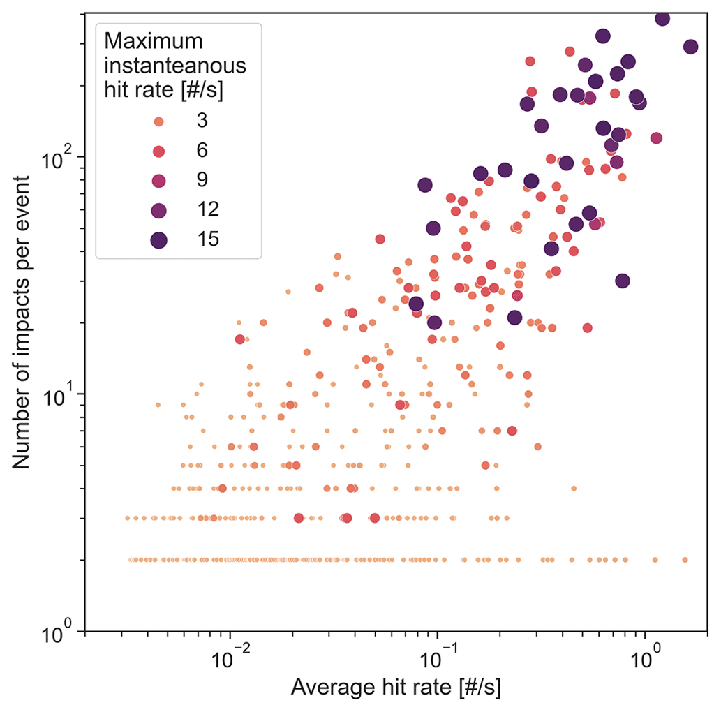
Figure 11 Scatterplot of hail events for t_mb=10 min organized by the average hit rate (x axis) and number of impacts (y axis). The colour and size represent the maximum instantaneous hit rate of the event (larger values are represented by darker and larger dots).

3.3.3 Timing of the largest hailstone (D_max)

Figure 12 shows the distribution of the relative time when the largest hailstone (D_max) of the event hit the sensor for the four values of (t_mb). For a given event, a value of 0.5 would mean that the D_max hailstone hit the sensor in the middle of the event.

If the D_max hailstone hit the sensor randomly during an event, then the distribution of Fig. 12 would be uniform, with a 0.5 median relative time. However, as the number of impacts per event increases, the time at which D_max occurs comes closer to the event's start. For dense hail events (>25 impacts), D_max occurs within the first third of the event for 50 % of the events (0.34 median relative time). This means that it is more likely that D_max would be recorded at the beginning of the event. This could be explained by the fact that the larger the hailstone, the faster it falls, and therefore, larger hailstones should hit the ground before smaller ones.

However, as stated in Sect. 3.3.2, a hailstreak can be recorded at any stage of its lifecycle and at any relative position. If the hailstones produced during a streak were first small, then grew in size to reach a maximum diameter (phase of increasing diameter), and then became smaller (phase of decreasing diameter), and if both phases lasted equally long, then we would expect that the relative time of D_max would be equally distributed, with a mean of 0.5 for a large number of observed events. Indeed, in the phase of increasing diameters, the sensor would measure D_max in the middle or towards the end of the event. In the phase of the decreasing diameter, the sensor would measure D_max at the beginning. Our results suggest that it is more likely for D_max to be recorded at the beginning of the event.

This is consistent with the hypothesis formulated in Sect. 3.3.2, which argues that most hailstones are reaching the ground in a short and intense maturing phase, followed by a few remaining hailstones during a longer dissipating phase. In such a model, the odds of observing any hailstone (including the one with the largest diameter) at the beginning of the event is increased.

We also note that, for hail events with few impacts (two to five impacts), it is difficult to reach any conclusion, as the number of hailstones observed is very small for each event (not shown).

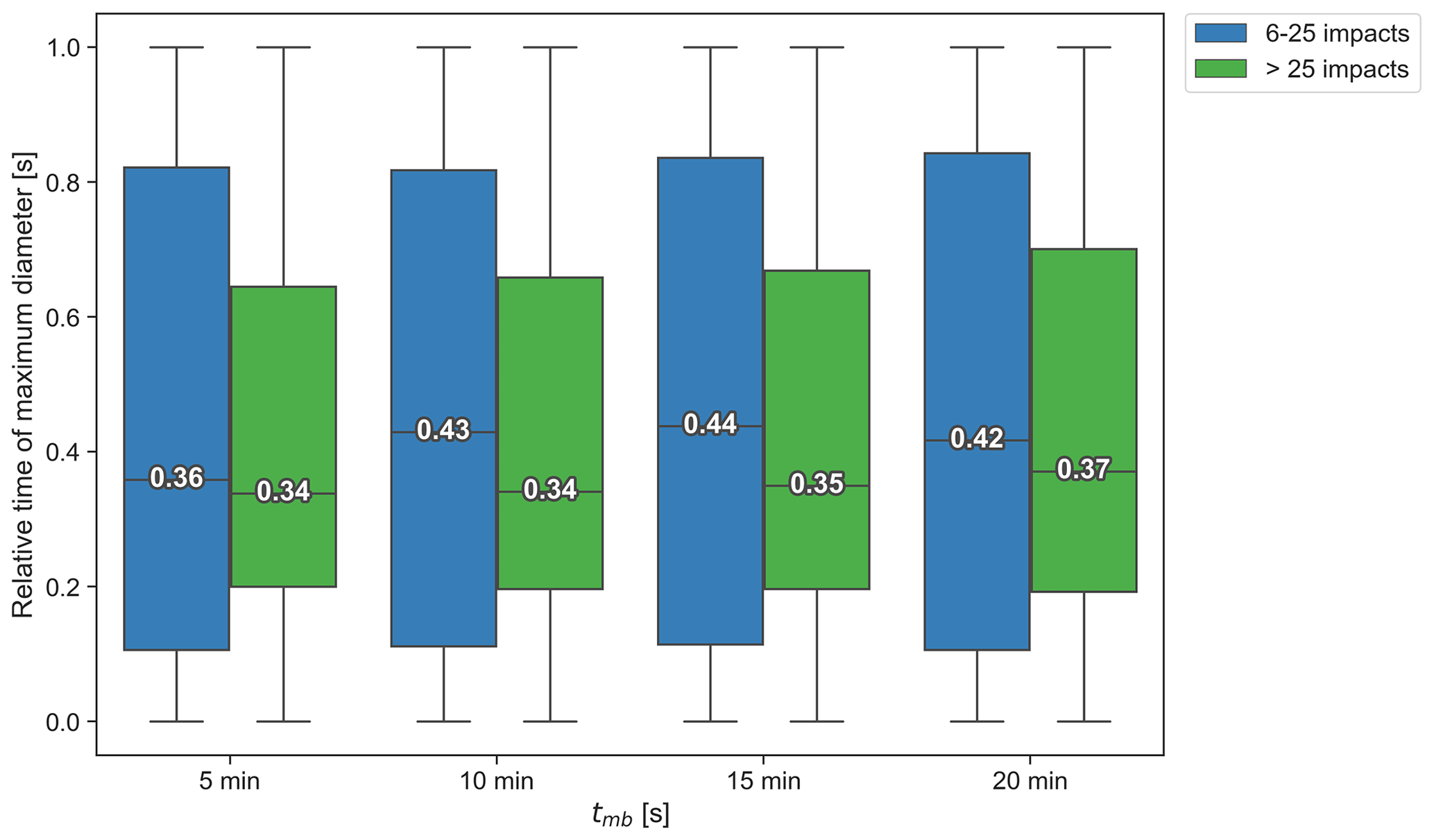
Figure 12 Box plots of the relative time of occurrence of the largest hailstones during an event for t_mb values of 5, 10, 15, and 20 min that are each stratified by impacts numbers (colours). The numbers show the median relative time in seconds.

4 Summary, conclusions, and outlook

We present an analysis of automatic hail sensor data from a national network in Switzerland. Our study is based on a sample of about 12 000 hailstone impacts and 500 hail events, gathered during three to five hail seasons, depending on the sensor location. The capacity of the sensors to record the precise timing of hailstone impacts and their kinetic energy opens new research avenues with respect to the local hailstorm duration and lifecycle and time-resolved hailstone size distributions.

As with any measurement device, the sensors come with some limitations; these include an uncertainty of the diameter measurement (it is recommended to work with 5 mm size bins), a diameter-dependent dead time ranging from 0.064 to 0.5 s, which can result in 4 % to 4.6 % of missed impacts, and the possible recording of impacts that are not due to hail. This accuracy is sufficient for our study.

The impacts of those limitations could be reduced by using the hail sensors together with other hail measurement devices. The number and size of the missed impacts could be estimated by using hailpads in conjunction with hail sensors and comparing their size distribution. This could also help reduce the uncertainty in the diameter measurements. The use of advanced radar-based hail algorithms (such as differential reflectivity (Z_DR) columns or hydrometeor classification; see, e.g., Besic et al., 2016) could help discriminate the impacts not due to hail.

More specifically, we recommend performing the field calibration and resetting the minimum threshold right before installing or using the sensor in a field campaign to obtain the most precise measurements. If two sensors are deployed at the same location, then it could also be interesting to set a signal threshold corresponding to diameters lower than 5 mm on one of them to observe graupel.

We showed that, despite their different measurement approaches, hail sensors and hailpads measure the same hail size distributions, as confirmed by the similar fits of Eqs. (5) and (4) and several statistical tests.

We discuss the time series of the impacts recorded by the hail sensors to illustrate that the definition of a hail event is sometimes not trivial and propose a method using a single parameter t_mb to characterize the events. We test values of t_mb between 5 and 20 min. The timing of hailstone impacts can be used to extract the local duration of hailfalls. The majority of local hailfalls last just a few minutes (less than 4.4 min for t_mb=5 min and less than 7.7 min for t_mb=20 min). Those durations are slightly higher than the previously reported durations by human observers in the literature for other countries. The difference might be due to the high sensitivity of the hail sensor, which records every single impact, compared to a human observer, who can miss those single impacts. To focus on the bulk of hail events, we looked at the cumulative time distribution of impacts (CTDIs) and found that the majority of impacts occurred in less than 3.3 min (t_mb=5 min) to less than 4.7 min (t_mb=20 min), a range of duration that is comparable to the existing literature. The fact that the local hailfall duration is usually shorter than 5 min should also be considered when examining radar-based data, as their time resolution in Switzerland is 5 min. The most considerable sensitivity of the hailfall duration and CTDIs is observed when t_mb increases from 5 to 10 min, whereas there is very little change when t_mb increases from 15 to 20 min. Therefore, we suggest using a 10 to 15 min value for t_mb in further studies.

The majority of the hailstone impacts is on average concentrated at the beginning of an event. This suggests that most events are composed of a rapidly increasing and short phase of high hailstone density at the beginning of the event, followed by a longer phase with low hailstone density. Most hailstones, including the largest, fall during the first phase of high intensity, while a few remaining and smaller hailstones fall in the second low-density phase. This interpretation of the observations remains a hypothesis and should be further investigated.

Finally, we observed that the hail events with the largest number of impacts also have the largest peak intensity, as measured by the maximum instantaneous hit rate.

The sensor data provide interesting results, but more observations are needed to reach more robust conclusions. The sensor network in Switzerland will be operating for at least 4 more years, and other countries have started or have considered using the same hail sensor model for national networks.

Our comparison of hail sensor and hailpad observations is done using samples coming from two different regions composed of a different set of hailstorms. Ideally, hail sensors and hailpads should be paired at the same locations for comparison. Used in pairs, they would not only give a more complete view of the hail size distribution but also would allow for the identification of possible differences in the measurements between the two devices and thus provide a better understanding of their respective biases.

We used the output diameters of the hail sensor as provided by the manufacturer in the present study. Such diameters were estimated using the approximation that hailstones are spherical, which is not always the case, especially for large hailstones. Pairs of hailpads and hail sensors could be used to investigate more advanced non-spherical approaches (e.g. Heymsfield et al., 2018; Shedd et al., 2021). For example, the distribution of aspect ratios could be inferred from the hailpad measurements and used as input when estimating the hailstone dimensions from the kinetic energy measurements of the hail sensors.

Hail is a rare phenomenon that is extremely localized in both space and time and is therefore challenging to observe. Automatic hail sensors allow us to observe hail extremely precisely in time – something which was difficult, if not impossible, to do with the existing devices. However, the sensors should be used together with other measurement sources such as hailpads, (mobile) radar, crowdsourced observations, or drone aerial measurements. Such a combination would allow us to obtain the most comprehensive picture of a hailstreak and its related hailstone distribution in further research.