the Creative Commons Attribution 4.0 License.
the Creative Commons Attribution 4.0 License.
 | 10 Aug 2023
Particle inertial effects on radar Doppler spectra simulation
Pavlos Kollias
Radar Doppler spectra observations provide a wealth of information about cloud and precipitation microphysics and dynamics. The interpretation of these measurements depends on our ability to simulate these observations accurately using a forward model. The effect of small-scale turbulence on the radar Doppler spectra shape has been traditionally treated by implementing the convolution process on the hydrometeor reflectivity spectrum and environmental turbulence. This approach assumes that all the particles in the radar sampling volume respond the same to turbulent-scale velocity fluctuations and neglects the particle inertial effect. Here, we investigate the inertial effects of liquid-phase particles on the forward modeled radar Doppler spectra. A physics-based simulation (PBS) is developed to demonstrate that big droplets, with large inertia, are unable to follow the rapid change of the velocity field in a turbulent environment. These findings are incorporated into a new radar Doppler spectra simulator. Comparison between the traditional and newly formulated radar Doppler spectra simulators indicates that the conventional simulator leads to an unrealistic broadening of the spectrum, especially in a strong turbulent environment. This study provides clear evidence to illustrate the droplet inertial effect on radar Doppler spectrum and develops a physics-based simulator framework to accurately emulate the Doppler spectrum for a given droplet size distribution (DSD) in a turbulence field. The proposed simulator has various potential applications for the cloud and precipitation studies, and it provides a valuable tool to decode the cloud microphysical and dynamical properties from Doppler radar observation.
- Article
(2722 KB) - Full-text XML
- BibTeX
- EndNote


The radar Doppler spectrum represents the frequency (velocity) distribution of the backscattered radar signal at a particular range. For a vertically pointing radar, the Doppler spectrum provides the distribution of the backscattered signal over a range of Doppler velocities, whose value depends on the dynamical (i.e., vertical air motion) and cloud microphysical (i.e., concentration and size of hydrometeors) properties within the radar sampling volume. A variety of research applications that utilize the full radar Doppler spectrum have been developed. For instance, Doppler spectrum can be used to retrieve rain droplet size distribution (DSD; Atlas et al., 1973), remove clutters and identify hydrometeor signals (Williams et al., 2018; Luke et al., 2008; Moisseev and Chandrasekar, 2009), identify the stage of drizzle development (Zhu et al., 2022; Acquistapace et al., 2019), retrieve vertical air motion (Kollias et al., 2002; Williams, 2012; Zhu et al., 2021), characterize the melting-layer properties (Li and Moisseev, 2020; Mróz et al., 2021), and improve the representation of cloud microphysical process in the model (Kollias et al., 2011b). Combined with the depolarization capability, the Doppler spectrum can also be used for cloud-phase classifications and to investigate ice-cloud microphysical process (Luke et al., 2010, 2021; Kalesse et al., 2016; Oue et al., 2018). The forward Doppler spectra simulator can further be utilized to simulate radar observation from the modeling output to evaluate the model performance (Oue et al., 2020; Mech et al., 2020; Silber et al., 2022). The list of widely used applications of the Doppler spectrum in the cloud–precipitation research mentioned above is by no means exhaustive.
Despite the extensive applications, an unambiguous interpretation of radar Doppler spectrum still remains a challenging task in the cloud radar community. One important reason is a lack of full understanding of the entanglement between the hydrometeor microphysics and environmental dynamics as well as their manifestation on the Doppler spectrum morphology (Kollias et al., 2002). More specifically, the Doppler spectrum width is mainly contributed by the spread of the still-air hydrometeor terminal velocity, the horizontal and vertical wind shear within the radar observation volume, and the environmental turbulence; while the Doppler frequency shift is a combined measure of the air motion and the falling velocity of particles (Doviak, 2006). A successful separation of the microphysical and dynamical contributions to Doppler spectrum is essential to reduce retrieval uncertainties and to better characterize the cloud–precipitation properties (Zhu et al., 2021).
Doppler spectrum simulators have been invaluable for the interpretation of the radar Doppler spectrum shape (Capsoni et al., 2001; Oue et al., 2020; Kollias et al., 2011a; Maahn et al., 2015). Traditionally, the impact of turbulence on the shape of the radar Doppler spectrum is represented by the convolution of the still-air (no-air motion) hydrometeor reflectivity spectrum with a Gaussian distribution (Gossard and Strauch, 1983). The width of the Gaussian distribution is parameterized as a function of the radar parameters and the turbulence intensity often represented in terms of eddy dissipation rate (Borque et al., 2016). This approach is only valid under the assumption that the droplet inertial effect is negligible and droplets with different sizes can follow the environmental wind field exactly. In reality, however, big droplets with large inertia cannot follow the rapid change of the wind velocity field like small droplets do (Yanovsky, 1996; Lhermitte, 2002). Not accounting for the particle inertial effect can lead to a misinterpretation of the Doppler spectrum and cause large uncertainties for retrieval products (Nijhuis et al., 2016).
Several physics-based frameworks have been proposed to simulate the droplet motions in the turbulence field (Khvorostyanov and Curry, 2005; Lhermitte, 2002). Here, the approach proposed by Lhermitte (2002) is used to illustrate the droplet inertial effect and to investigate this effect on the radar Doppler spectrum. In detail, we aim to answer the following questions. (1) How does inertia affect the response of a droplet in a fluctuating turbulent wind field? (2) Is this effect significant on the simulated and observed radar Doppler spectrum? (3) How can we account for the droplet inertia in radar Doppler spectrum simulators? Building on these investigations, a new approach to generate radar Doppler spectrum is described.
The structure of this paper is organized as follows: Sect. 2 describes the physical modeling framework used to simulate the liquid droplet motion and to illustrate the droplet inertial effect in a turbulent environment. Section 3 proposes the physics-based Doppler spectrum simulator and compares the emulated spectra to the ones generated from the traditional method. In Sect. 4, one observed Doppler spectrum is used as an illustrative example to compare the Doppler spectrum generated from the two simulators. Section 5 shows the conclusions of this study, which are followed by a discussion.
In this section, a physics-based simulation (PBS) framework used to illustrate the droplet inertial effect in a turbulent environment is presented. First, we will introduce the equations used to describe the velocity of droplets moving in the air. Then, a generated turbulent wind field is applied to the simulation framework to illustrate the droplet inertial effect and the potential implication on the generated Doppler spectrum.
2.1 Motion of droplets in the air
The fundamental dynamical framework of describing the motion of droplets in the air is adapted from Lhermitte (2002, p. 81). Assuming a liquid droplet with diameter D, the motion of the droplet in the air can be described as follows:
where m is the droplet mass, VD is the droplet velocity, F is the drag force exerted by wind expressed as
where Cd is the wind drag coefficient, ρa is air density, and S is the droplet cross section perpendicular to wind direction; Vw is wind velocity and (Vw−VD) indicates droplet velocity with respect to air. In a turbulent environment, Vw cloud be either positive or negative, thus the exerted wind can either accelerate or decelerate the droplet velocity. To this end, the sign function sgn(Vw−VD) is included to account for the wind drag force direction.
For spherical droplets, S can be calculated as
and droplet mass (m) is calculated as
where ρl is liquid water density.
The only unknown factor is the drag coefficient Cd, which should be derived from the experiment. Numerous studies have been conducted to measure the sphere terminal velocity in fluid and estimate Cd as a function of the Reynolds number (Re) (Schlichting and Kestin, 1961; Lapple and Shepherd, 1940; Haider and Levenspiel, 1989). However, the derived Cd–Re relationships in the previous studies are applied for rigid spherical particles. For the rain droplets with large diameters, the droplet is distorted and the exerted drag coefficient for a given Re deviates from the rigid sphere. To this end, the drag term of the rain droplet is obtained from the measurement of the terminal velocity of liquid droplets. Here, we adapt the experiment data from Gunn and Kinzer (1949); in their study, Cd and Re are estimated for liquid droplets with a diameter ranging from 100 µm to 5.8 mm. The experiment-derived Cd and Re are shown in Fig. 1. We further fit the data with a fifth-degree polynomial (red line) to estimate Cd for a given Re:
where the Reynolds number Re is represented as
where μ is the air dynamic viscosity. The values used for ρa, ρl, and μ are 1.22 kg m−3, 1000 kg m−3, and kg m−1 s−1, corresponding to the atmospheric environment of 15 ∘C and 1000 hPa.
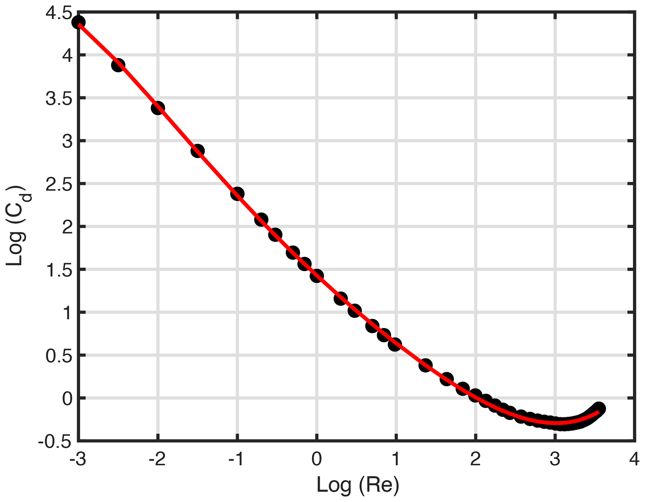
Figure 1The black dots represent the experiment-derived Cd and Re adapted from Gunn and Kinzer (1949). The red line is a fifth-degree polynomial fitting function.
Combining Eqs. (1)–(6), a set of ordinary differential equations is constructed, and the droplet velocity (VD) for a given droplet with diameter D as a function of time can be resolved numerically for a given wind field (Vw).
2.2 Illustration of droplet inertial effect
We first illustrate the inertial effect by calculating the motion of droplets using a constant wind velocity. For simplicity, here we assume all the droplets are moving horizontally, thus the gravity (mg) is neglected in Eq. (1). Seven droplets with diameters of 10 µm, 50 µm, 100 µm, 500 µm, 1 mm, 2 mm, and 5 mm are selected to cover the size range of cloud droplets, drizzle, and raindrops. The initial velocity of all the droplets is 0 m s−1, a constant wind velocity of 10 m s−1 is exerted upon the droplets when t>0 s. Due to the wind drag force, droplets start to move but with different accelerations depending on droplet inertia: droplets with small inertia are accelerated more quickly than larger ones. This effect is clearly illustrated in Fig. 2: droplets with a diameter of 10 µm quickly reach the wind velocity within only 0.002 s, while droplets with 1 and 5 mm need 5 and 50 s, respectively, to adjust their motion to the exerted wind velocity. The different response time of droplets with different sizes to the exerted wind velocity suggests that small droplets are more capable of following the velocity variation than their large counterparts.
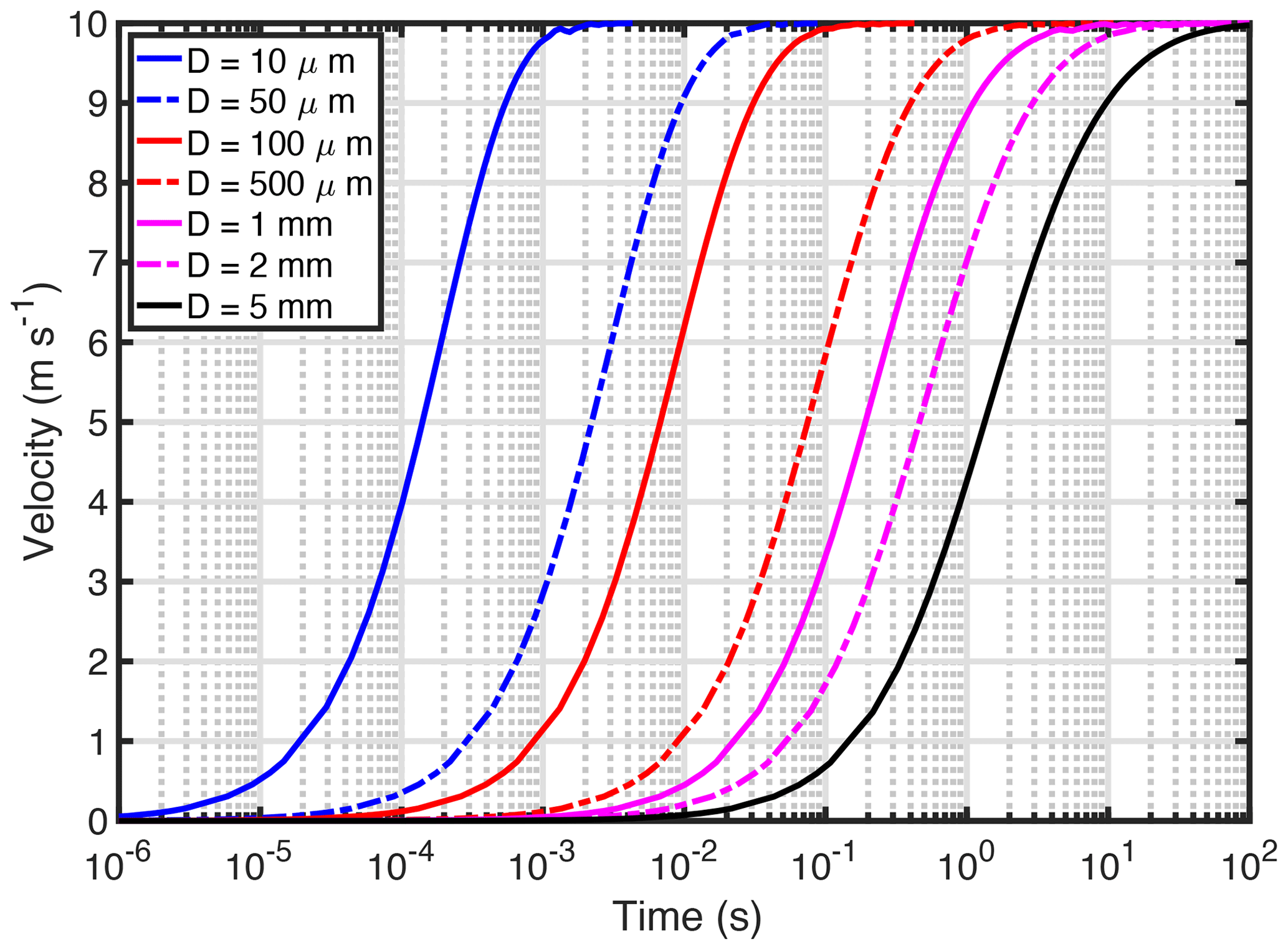
Figure 2Velocity of droplets with diameter of 10 µm (solid blue line), 50 µm (dash-dotted blue line), 100 µm (red line), 500 µm (dash-dotted red line), 1 mm (solid magenta line), 2 mm (dash-dotted magenta line), and 5 mm (solid black line) as a function of time after exerted by a constant wind with a velocity of 10 m s−1.
In real atmosphere, air velocity is not constant but fluctuates with time as a representative of turbulent nature. In this study, we adapt the approach proposed by Deodatis (1996) by using the spectral representation method (SRM) to generate the turbulent wind field based on a predefined Von Karman energy spectrum. The SRM is widely used in the wind engineering community due to its high accuracy, simplicity, and computational efficiency (Shinozuka and Deodatis, 1991; Zhao et al., 2021). Here, the 1-D turbulent wind is generated with 2 Hz sampling frequency, 1000 s duration, and with a standard deviation of 0.3 m s−1; the codes being applied to generate the wind can be accessed from Cheynet (2020). The selection of the 0.3 m s−1 standard deviation is based on a quantitative estimation of cloud radar observation under a typical cloudy environment. Specifically, for the convective cloud system with eddy dissipation rate (ε) of m2 s−3 (Mages et al., 2023), the turbulence-contributed Doppler spectrum width (σt) from a vertical pointing radar with 30 m range resolution (ΔR) and 0.3∘ beamwidth (θ) at 1 km height is estimated to be 0.27 m s−1 based on the equation from Borque et al. (2016):
where α is the Kolmogorov constant of 0.5, , , θ is the one-way half-power width with unit of radian, and z is height above surface.
The spectrum and time series of the generated air velocity are shown in Fig. 3: the turbulence spectrum (Fig. 3a) characterizes the typical inertial subrange of the turbulence scale with a standard deviation of 0.3 m s−1 (Fig. 3b).
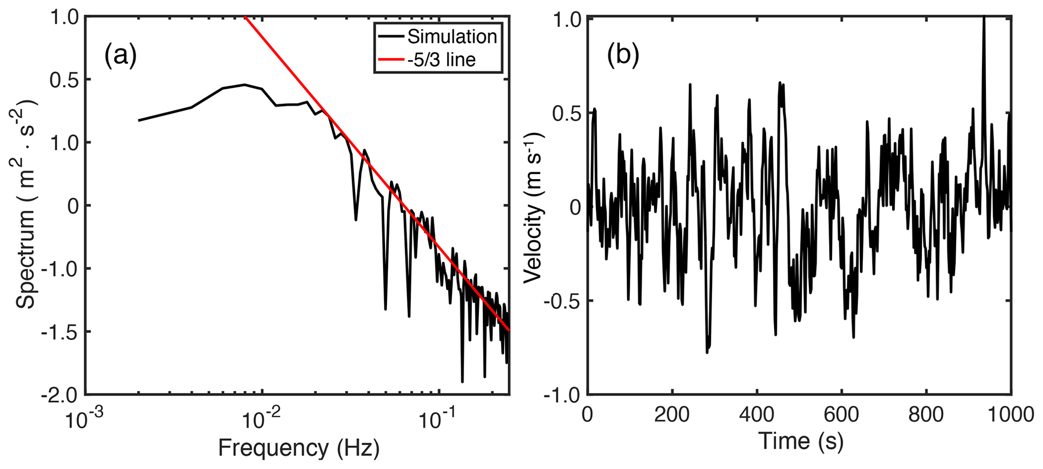
Figure 3(a) Spectrum of the simulated turbulence (black line), red line represents the slope. (b) Time series of vertical velocity for the simulated turbulence.
The generated air velocity is assigned to Vw in Eq. (2) to simulate the motion of droplets with initial velocity set as 0 m s−1. Figure 4a shows the time-dependent velocity of droplets with a selected diameter of 0.5, 1, 2, and 3 mm. Droplets with different sizes respond differently with the change of wind velocity, and there are two notable characteristics due to the inertial effect (highlighted in the black oval in Fig. 4a). First, large droplets need longer time to adjust to the wind velocity, thus there is a distinct time lag when the peak velocity is reached for different particles. Second, in addition to the time lag, the peak velocity reached by the large droplets is smaller than that of the small droplets. Here, we use the correlation coefficient between the actual wind velocity and the droplet velocity to quantify the inertial effect. A correlation coefficient of 1 represents droplets that can follow the wind velocity exactly, and a correlation coefficient less than 1 indicates a time-lag effect between the wind and droplet velocity due to droplet inertia. Figure 4b shows that the correlation coefficient is close to 1 when the droplets are smaller than 50 µm but it decreases dramatically as droplet size increases. The correlation coefficient drops to 0 when diameter reaches 2000 µm. In addition, for droplets with diameters smaller than 300 µm, the standard deviation of the actual droplet velocity is 0.29 m s−1 (blue curve, Fig. 4b), which is close to the standard deviation of the background wind field (0.3 m s−1). As the droplet size increases, the velocity variation decreases due to the droplet inertial effect.
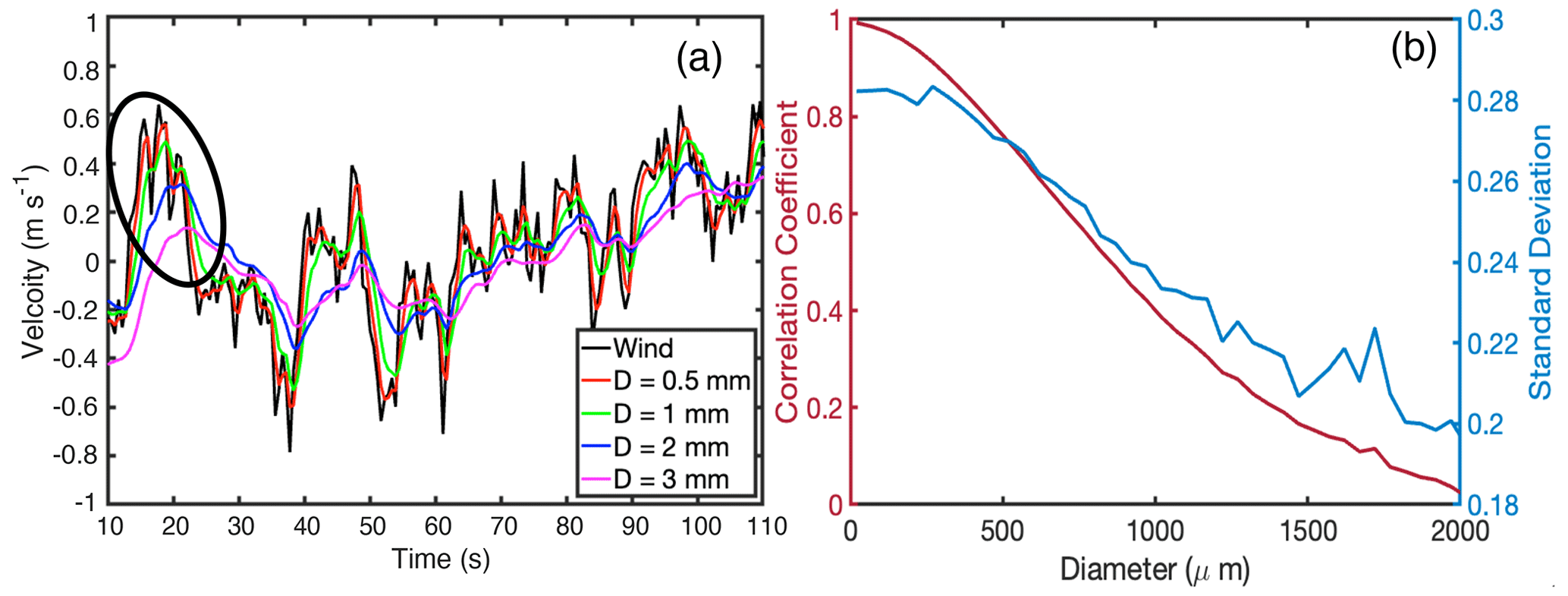
Figure 4(a) Generated wind velocity field (black line) and the simulated velocity for particles with a diameter of 0.5 mm (red line), 1 mm (green line), 2 mm (blue line), and 3 mm (magenta line) from 10 to 110 s. The black oval indicates the period showing the droplet inertial effect. (b) Left axis: correlation coefficient between wind field and droplet velocity for different droplet sizes; right axis: standard deviation of the droplet velocity with different droplet sizes. Only droplets with a size from 0 to 2000 µm are shown for the sake of clarity.
The simulation results shown in Fig. 4 suggest that droplets with diameter smaller than 300 µm are less affected by inertia and can quickly adjust their velocity to the imposing wind field, and thus, small cloud droplets can be treated as perfect air tracers (Kollias et al., 2001). On the other hand, large droplets (D>0.5 mm) exhibit a time lag in their response to the air motion and an amplitude reduction (inertia-based filtering). As the observed Doppler velocity is a combined measure of the droplet velocity and the ambient air motion, this droplet inertial effect is expected to have a considerable effect on the generated radar Doppler spectrum. In the following section, we will illustrate how the radar Doppler spectrum is affected by droplet inertia and how to account for this effect using a new radar Doppler spectrum simulator.
Two methodologies for simulating the radar Doppler spectrum for a given DSD and turbulent conditions are used here. The first approach is the traditional one. All droplets, independent of their sizes, are assumed to have no inertial effects and thus act like perfect tracers. In this case, the radar Doppler spectrum in a turbulent environment is represented through the convolution of a Gaussian distribution and the radar Doppler spectrum in still air, which is only determined by the hydrometeor DSD (Gossard, 1988; Kollias et al., 2011a; Zhu et al., 2021). A brief overview of the traditional method is described in Sect. 3.1.
3.1 Traditional Doppler spectrum simulator
For a given DSD described by a number concentration N(D) per unit of volume, the radar reflectivity dη(D) (m2 m−3) from particles with a diameter between D and D+dD can be expressed as in Lhermitte (2002, p. 228):
where σb(D) is the backscatter cross section (m2) of a particle with diameter D in meters. The Mie scattering theory is used to estimate σb(D). In this formulation, the radar power spectrum distribution is provided in terms of particle size. The profiling radar does not observe the backscattered radar power energy spectrum dη(D) but the radar Doppler spectrum density Sq(Vt), where Vt is the droplet still-air terminal velocity. The conversion from droplet size to velocity requires a Vt(D) relationship. Here, the function proposed by Lhermitte (2002, p. 120) is used to estimate Vt as a function of droplet diameter (D):
where the units of D and Vt are in centimeters (cm) and centimeters per second (cm s−1) respectively. Subsequently, the radar Doppler spectral density Sq(Vt) is given by
where is estimated from Eq. (9).
The Sq(Vt) is the still-air radar Doppler spectrum where the only velocity contribution is the droplet still-air terminal velocity. In the real atmosphere, the observed velocities from the radar include the turbulent motions with scales larger or smaller than that of the radar sampling volume (Kollias et al., 2001; Borque et al., 2016). The contribution of turbulence on Doppler spectrum broadening is commonly parameterized as σt. It is important to note that the σt value also strongly depends on the radar sampling characteristics (Kollias et al., 2005). For the same EDR value, σt is lower for radar systems with a short time dwell, narrow beamwidth, and short pulse length (Borque et al., 2016). The σt is typically used to introduce the effect of turbulence on the radar Doppler spectrum. Under the assumption of isotropic turbulence, the distribution of the turbulent motions within the radar sampling volume can be approximated using a Gaussian function:
Its impact on radar Doppler spectrum is formulated by the convolution between Sq(Vt) and G(v) (Gossard and Strauch, 1983) as
3.2 Physics simulation based Doppler spectrum simulator
In this approach, instead of using a Gaussian distribution to parameterize turbulence field and applying the convolution process to represent the interaction between DSD and environmental turbulence, the radar Doppler spectrum is generated using a large number of simulated droplet velocities during a given simulation period. Specifically, for droplets with diameter D moving in a turbulent flow, the droplet velocity at each specific time can be numerically resolved as V(Dt) based on the ordinary differential equations described in Sect. 2.1.
The radar Doppler spectrum density at each time step St(v) can be directly estimated as
where represents the diameter of the particle with velocity within the predetermined Doppler velocity interval at each time step; and indicate the number concentration and the backscatter power corresponding to each diameter. The predetermined Doppler velocity Vi is dependent on the radar configuration of the Nyquist velocity (Vnyquist) and the number of the fast Fourier transform points (NFFT):
The final Doppler spectrum can be obtained by averaging St(v) during the simulated period:
where Nt denotes the total simulation time steps:
where T and f are the simulated time and the sampling frequency of the generated turbulent wind field.
It is noted that the emulated radar Doppler spectrum is dependent on the generated turbulent flow, which is controlled by three parameters: time duration (T), sampling frequency (f), and standard deviation (σ); σ quantify the turbulence intensity, while T and f determine the total emulated time steps. Here, we use the typical cloud radar configurations to guide the choice of T and f. Specifically, T is set as 2s and f is set as 20 Hz to accommodate the cloud radar operated at the Atmospheric Radiation Measurement (ARM) program with approximately 40 spectra being averaged in 2 s (Kollias et al., 2005).
3.3 Doppler spectra comparison from two simulators
Both simulators described above are applied to emulate the Doppler spectrum observed by a 94 GHz (W-band) profiling cloud radar for a given DSD and for a set of different turbulent environments. The Nyquist velocity is set as ±12 m s−1 and a 512-point fast Fourier transform (FFT) is used to generate the radar Doppler spectrum. The Marshall–Palmer exponential DSD (Marshall and Palmer, 1948) with is used to represent the DSD in the radar sampling volume. The values of the intercept parameter N0 and the slope factor Λ are chosen to be 0.08 cm−4 and 15 cm−1, respectively. The droplet diameter ranges from 10 to 4000 µm with a bin size of 1 µm. The selection of W-band radar and the use of a rain DSD is because it is well known that the W-band radar Doppler spectrum in rain has distinct features which allow us to pinpoint the Doppler spectrum morphology. Specifically, according to the Mie scattering theory, radar backscattering cross section varies in an oscillatory manner with particle size (Mie, 1908). With the 3.2 mm wavelength radar, the backscattering cross section as a function of droplet size is characterized as several local minimal values with diameters of 1.66 and 2.86 mm, which correspond to still-air terminal fall velocity of 5.83 and 7.89 m s−1, respectively. This unique feather is known as “Mie notches” in the radar Doppler spectrum (Kollias et al., 2002, 2007; Courtier et al., 2022). In the simulation, turbulence field is generated with 20 Hz frequency (f), 100 s duration (T), and a standard deviation (σ) of 0.05, 0.25, 0.35, and 0.45 m s−1, respectively. The reason for applying different turbulence settings is to better illustrate the droplet inertial effect under different turbulent environments. It is expected that with increasing turbulence intensity the droplet inertial effect will be manifested in larger differences between the generated radar Doppler spectrum from the two methods.
When solving the ordinary differential equations described in Sect. 2.1, the initial droplet velocity is set as 0 m s−1; thus, at the beginning of the simulation, the droplet gravity force is greater than the wind drag force; the droplets will accelerate until their terminal fall velocity is reached, after which the droplets fluctuate around the terminal fall velocity with variations induced by the exerted wind. The radar Doppler spectrum should be estimated after the steady state is reached. Here, we split the 100 s simulated period into two parts: the first 40 s is the “speed-up” time which allows the droplets of different sizes to adjust to their steady state; the remaining 60 s is used for Doppler spectrum emulation. Specifically, each Doppler spectrum is estimated within a 2 s interval as illustrated in Sect. 3.2, then the generated 30 Doppler spectra in the 60 s are further averaged to produce the final Doppler spectrum. This final average step is used to smooth the Doppler spectrum generated in a short period (2 s) during which the averaged exerted wind may have a non-zero value.
The emulated Doppler spectrum from two methods with four turbulence settings is shown in Fig. 5. In a turbulent environment with σt of 0.05 m s−1 (Fig. 5a), the two simulated spectra (red and blue lines in Fig. 5a) and the Doppler spectrum without turbulence broadening (black line) almost overlap, indicating that the radar Doppler spectrum shape is dominated by the DSD shape and the droplet still-air terminal fall velocity in weak turbulent conditions. When σt equals 0.25 m s−1, the broadening of the right edge of the radar Doppler spectrum from the physics-based simulation(PBS) approach (red line in Fig. 5b) is less than that produced with the convolution approach (blue line in Fig. 5b). As σt increases to 0.35 m s−1, a large difference between the right edges of the spectra from the two simulators can be clearly identified. When σt reaches 0.45 m s−1, the right edge velocity difference between two spectra is larger than 1 m s−1. Overall, the right edge from the PBS-generated Doppler spectrum is more steep than that from the convolution-based approach, illustrating that large droplets cannot follow the rapidly changed turbulence field due to the inertial effect. Another notable finding is that the left part of the Doppler spectra (velocity smaller than 4 m s−1) from two simulators almost overlap with each other in different turbulence scenarios, as this part of the spectrum is mostly contributed by small droplets with negligible inertial effect, thus the corresponding Doppler spectrum can be adequately represented by the convolution process.
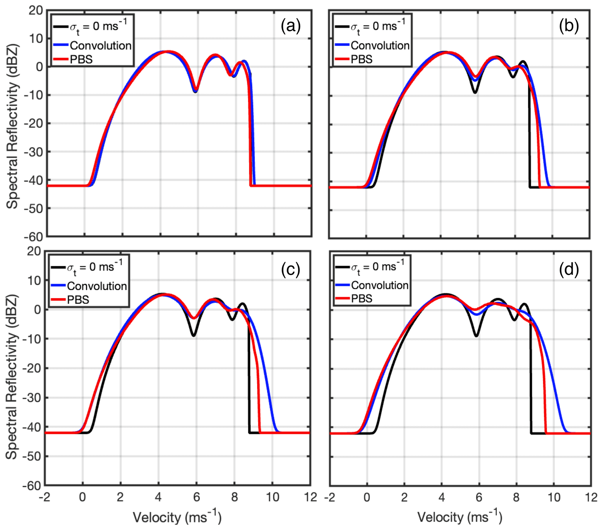
Figure 5Doppler spectrum generated by the convolution-based (blue line) and physics-based simulation (PBS) (red line) approach for turbulent standard deviation with (a) 0.05 m s−1, (b) 0.25 m s−1, (c) 0.35 m s−1, and (d) 0.45 m s−1. The black line represents the generated Doppler spectrum where σt=0 m s−1. Positive velocity indicates downward motion.
Comparing the three generated Doppler spectra in Fig. 5, we can clearly identify the effect of droplet inertia on Doppler spectrum morphology under different turbulent environments. In general, both simulators indicate a wider Doppler spectrum under a large turbulent condition but with different broadening magnitudes. The convolution-based approach generates a wider spectra in a more turbulent environment. This overestimation of the turbulence-broadening effect indicates that the convolution process used in the conventional simulator is unable to accurately represent the interaction between DSD and turbulence field. On the other hand, for the small droplets, the inertial effect is negligible and the generated Doppler spectra from the two approaches are consistent with each other. It is therefore concluded that the convolution process can simulate the Doppler spectrum for the light drizzle precipitation which mostly occurs in marine boundary layer clouds, but it is inadequate to emulate Doppler spectrum for the heavy precipitation in deep convection, especially in the presence of a strong turbulent environment.
In this section, we will present an illustrative example by using one observed Doppler spectrum to evaluate the performance of the simulators. The observed Doppler spectrum is obtained from the W-band ARM Cloud Radar (WACR) at the ARM Southern Great Plain (SGP) observatory during a heavy precipitation period on 9 May 2007. For the WACR, the maximum unambiguous velocity is 7.8 m s−1, which is smaller than the still-air terminal velocity of droplets with diameter larger than 3 mm and lead to velocity folding. Here, the velocity de-aliasing process is performed to reconstruct the Doppler spectrum with velocity from 0 to 11 m s−1. The observed Doppler spectrum is further calibrated from the displacement caused by vertical air motion by pinpointing the location of the first Mie notch of the Doppler spectrum to 5.83 m s−1 (Kollias et al., 2002). To simulate the Doppler spectrum, the hydrometeor DSD and the turbulence-broadening term (σt) are needed. Here, the rain DSD is observed from the impact disdrometer which can measure droplet diameters from 0.3 to 5.4 mm with 20 bins (Wang et al., 2021). The temporal resolution of the WACR and the disdrometer is 4.28 s and 1 min, respectively. To make the observation from two instruments comparable, the WACR-observed Doppler spectra are averaged over 1 min to coincide with the disdrometer observational period. For this example, we use the disdrometer-measured DSD from 05:44 to 05:45 UTC to simulate the radar Doppler spectrum and compare it with the one observed of WACR in the same period.
The observed DSD is shown in Fig. 6a, and the corresponding WACR-observed Doppler spectrum is shown as the black line in Fig. 6b. Based on the observed DSD, the radar Doppler spectrum for the droplets falling in still air is generated (not shown), from which the DSD-contributed Doppler spectrum width (σD) is estimated as 1.34 m s−1. Since the wind-shear-broadening contribution (σS) to the radar Doppler spectrum is generally smaller than σD and the turbulence broadening (σt) (Borque et al., 2016), here we neglect the σS contribution and estimate σt as
where σO is the observed Doppler spectrum width, which is 1.46 m s−1 in this example, and σt is estimated as 0.58 m s−1. To estimate the accuracy of σt, we further assume that the observed DSD is the only source of the uncertainty. Considering that the accuracy of the droplet size measurements of the disdrometer is approximately ±5 % (Wang et al., 2021), the uncertainty of σD and σt is estimated as 0.15 m s−1.
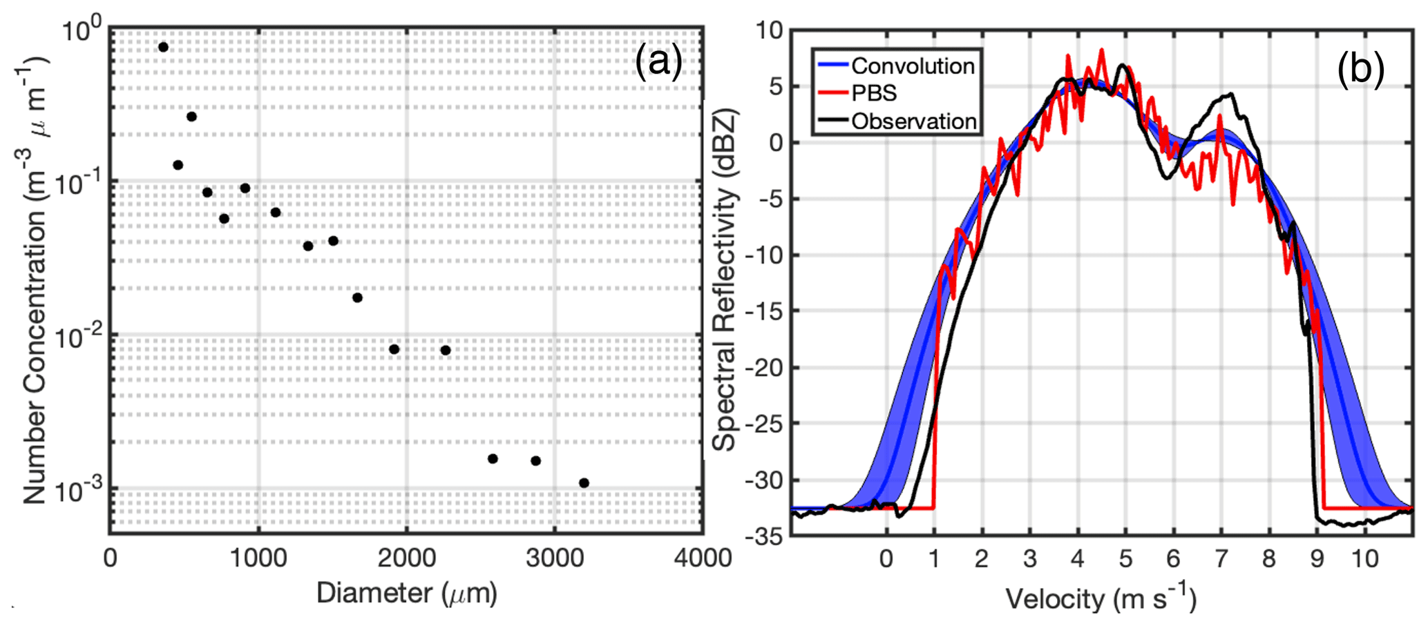
Figure 6(a) Black dots represent the observed raindrop number concentration from the disdrometer at 05:44 UTC on 9 May 2007 at the SGP site. (b) Doppler spectra simulated from the PBS method (red), convolution method (blue), and the observed spectrum from WACR (black line). The shaded blue region represents the uncertainty of the simulated Doppler spectrum produced by the uncertainty in σt based on the convolution method. Positive velocity indicates downward motion.
With the observed DSD and the estimated σt, the radar Doppler spectrum can be simulated. It is noted that large rain droplets falling in the air are nonspherical, thus backscattered power from an oblate droplet may be different to the one from a rigid liquid sphere. To this end, for the Mie scattering calculation, the axis ratio of the droplet with a diameter larger than 2 mm is considered a function of the diameter (D) in millimeters (Pruppacher and Beard, 1970):
The simulated Doppler spectrum from the convolution and the PBS methods are shown in Fig. 6b. It is noticeable that the Doppler spectrum from the PBS approach (red line) is more noisy than that from the convolution approach (blue line). This is due to the insufficient bin categories of the particles measured from the disdrometer. It is expected that by increasing the number of the measured particle size, the generated Doppler spectrum becomes more smooth. Nevertheless, it is still recognizable that both the morphology and the magnitude of the PBS-based spectrum right edge is more consistent with observation compared to the one generated from the convolution approach. Both of the simulators represent the first peak of the Doppler spectrum from 3 to 6 m s−1 very well, while neither of them generate a consistent second-peak morphology compared to observation. The left edge of the Doppler spectrum from the convolution-based approach is broader than the observation, while the PBS is unable to represent the Doppler spectrum smaller than 1 m s−1 due to the absence of droplets with a diameter smaller than 0.3 mm observed from the disdrometer.
The purpose of this Doppler spectrum comparison is not for a robust validation, but it is used as an illustrative example to show the morphology of the simulated Doppler spectrum based on real observations and to discuss the required measurements that would be used for a robust Doppler spectrum simulator validation. To a certain degree, a more consistent Doppler spectrum morphology is identified between the observation and the PBS simulator, especially for the right edge of the spectrum. However, great caution should be taken for further interpretation as both of the simulators cannot represent the left part of the Doppler spectrum and the second notches very well. This discrepancy is mainly because the observed DSD by the disdrometer may not provide an adequate representation of the hydrometeors that contribute to the Doppler spectrum observed by WACR. Specifically, there are three critical challenging issues that should be overcome before a solid and convincing evaluation effort of the Doppler spectrum simulator can be performed. (1) The disdrometer is located at the surface, while the lowest measurement height of WACR is 460m. When the rain droplets fall, droplets may collide, break up, and be advected from adjacent regions by the horizontal wind. Thus a large uncertainty is expected by using the surface-observed DSD to represent the hydrometeor distribution at 450 m above. (2) The observed DSD from the disdrometer only measures droplets with 20 size categories, which is insufficient for the physics-based simulation to generate a smooth and complete Doppler spectrum. (3) It is challenging for the uncertainty of the estimated σt to be well constrained due to the large uncertainty of the observed DSD mentioned above. A comprehensive and solid validation of the Doppler spectrum simulator requires simultaneous and well-aligned DSD and Doppler spectrum measurements, i.e., a large number of the measured droplet size categories and careful estimation of the environmental turbulence-broadening factors.
The radar Doppler spectrum offer unprecedented capabilities for studying cloud and precipitation microphysics. Recent advancements in radar technology and signal processing have enabled the continuous recording of high-quality radar Doppler spectra observations from a wide range of profiling radar systems (Kollias et al., 2005, 2016). Until now, the simulation of the radar Doppler spectra was based on well-established techniques (Gossard, 1988; Kollias et al., 2011a). However, the inertial effect of large droplets are typically neglected in the design of current simulators. Here, the impact of the liquid droplet inertia on the shape of the radar Doppler spectrum was investigated. A physics-based simulation framework is developed to simulate the droplets velocity in a given turbulent environment. It demonstrates that big droplets with large inertia will take longer time to adapt to the change of velocity field, indicating that large droplets are incapable of following the turbulent wind as small droplets do.
Building on the simulation framework, a new approach is proposed to emulate the Doppler spectrum by simulating the velocity of each droplet during the entire time domain. The simulated W-band radar Doppler spectrum is compared with the one generated from the traditional method for a typical DSD with four different turbulent environments. The comparison indicates that the traditional Doppler simulator generates an artificially broader Doppler spectrum without considering the inertial effect. This inertial effect becomes more noticeable as turbulence intensity increases. This finding suggests that special caution should be taken when applying convolution-based approaches to represent DSD turbulence interaction in heavy precipitation. In the case of light precipitation mostly happening in the marine boundary layer cloud, the droplet inertial effect on Doppler spectrum is negligible and the traditional simulator generates consistent results with the proposed simulator.
One WACR-observed Doppler spectrum collected from the ARM SGP observatory is compared with the simulated Doppler spectrum as an illustrative example to validate the fidelity of the simulator from the convolution and PBS approaches. The presented case shows that the proposed PBS generates a similar morphology of the right edge of the Doppler spectrum compared to the traditional simulator. However, both of the simulators fail to reconstruct the left edge and the second notch of the Doppler spectrum. These inconsistencies are due to the fact that the surface-based DSD from the disdrometer is inadequate to represent the hydrometeor observed by cloud radar at a high level. A careful and solid validation of the radar Doppler spectrum simulator would require co-aligned observations of DSD and Doppler spectrum including well-constrained turbulence-broadening estimations. Nevertheless, the proposed Doppler spectrum simulator, with the ability to simulate individual droplet motions and their manifestation on the Doppler spectrum, provides a valuable tool to improve the understanding of the Doppler radar observation from a fundamental physics perspective. We expect that this proposed Doppler spectrum simulation framework can stimulate more studies to better interpret the Doppler radar observation and to decode the microphysics and dynamics information concealed in the radar Doppler spectrum.
The codes of the proposed Doppler spectrum simulator can be accessed via https://doi.org/10.5281/zenodo.7897981 (Zhu, 2023).
Ground-based data were obtained from the Atmospheric Radiation Measurement (ARM) user facility, a U.S. Department of Energy's (DOE) Office of Science user facility managed by the Office of Biological and Environmental Research (Johnson et al., 2022, https://doi.org/10.5439/1025318; Wang, 2022, https://doi.org/10.5439/1025181).
ZZ implemented the method, performed the analysis, produced the figures, and wrote the initial draft of the paper. PK supervised and provided advice and guidance on all aspects of the analysis and contributed to the writing of the paper. FY advised on results interpretation and paper editing. All authors read the manuscript draft and contributed comments.
At least one of the (co-)authors is a member of the editorial board of Atmospheric Measurement Techniques. The peer-review process was guided by an independent editor, and the authors also have no other competing interests to declare.
Publisher’s note: Copernicus Publications remains neutral with regard to jurisdictional claims in published maps and institutional affiliations.
Zeen Zhu's contribution is supported by the Brookhaven National Laboratory via the Laboratory Directed Research and Development (grant no. LDRD 22-054). Pavlos Kollias and Fan Yang are supported by the U.S. Department of Energy (DOE) under contract no. DE-SC0012704.
This paper was edited by Stefan Kneifel and reviewed by Davide Ori and two anonymous referees.
Acquistapace, C., Löhnert, U., Maahn, M., and Kollias, P.: A New Criterion to Improve Operational Drizzle Detection with Ground-Based Remote Sensing, J. Atmos. Ocean. Tech., 36, 781+-801, 2019.
Atlas, D., Srivastava, R., and Sekhon, R. S.: Doppler radar characteristics of precipitation at vertical incidence, Rev. Geophys., 11, 1–35, 1973.
Borque, P., Luke, E., and Kollias, P.: On the unified estimation of turbulence eddy dissipation rate using Doppler cloud radars and lidars, J. Geophys. Res.-Atmos., 121, 5972–5989, 2016.
Capsoni, C., D'Amico, M., and Nebuloni, R.: A multiparameter polarimetric radar simulator, J. Atmos. Ocean. Tech., 18, 1799–1809, 2001.
Cheynet, E.: Wind field simulation (text-based input), Version 1.3, Zenodo [code], https://doi.org/10.5281/ZENODO.3774136, 2020.
Courtier, B. M., Battaglia, A., Huggard, P. G., Westbrook, C., Mroz, K., Dhillon, R. S., Walden, C. J., Howells, G., Wang, H., and Ellison, B. N.: First Observations of G-Band Radar Doppler Spectra, Geophys. Res. Lett., 49, e2021GL096475, https://doi.org/10.1029/2021GL096475, 2022.
Deodatis, G.: Simulation of ergodic multivariate stochastic processes, J. Eng. Mech., 122, 778–787, 1996.
Doviak, R. J.: Doppler radar and weather observations, Courier Corporation, ISBN-10: 0486450600, ISBN-13: 978-0486450605, 2006.
Gossard, E. E.: Measuring drop-size distributions in clouds with a clear-air-sensing Doppler radar, J. Atmos. Ocean. Tech., 5, 640–649, 1988.
Gossard, E. E. and Strauch, R. G.: Radar observation of clear air and clouds, Elsevier, ISBN-10: 0444421823, ISBN-13: 978-0444421821, 1983.
Gunn, R. and Kinzer, G. D.: The terminal velocity of fall for water droplets in stagnant air, J. Atmos. Sci., 6, 243–248, 1949.
Haider, A. and Levenspiel, O.: Drag coefficient and terminal velocity of spherical and nonspherical particles, Powder Technol., 58, 63–70, 1989.
Johnson, K., Nelson, D., and Matthews, A.: W-Band (95 GHz) ARM Cloud Radar (WACRSPECCMASKCOPOL). 2007-05-09 to 2007-05-10, Southern Great Plains (SGP) Central Facility, Lamont, OK (C1), ARM Data Center [data set], https://doi.org/10.5439/1025318, 2022.
Kalesse, H., Szyrmer, W., Kneifel, S., Kollias, P., and Luke, E.: Fingerprints of a riming event on cloud radar Doppler spectra: observations and modeling, Atmos. Chem. Phys., 16, 2997–3012, https://doi.org/10.5194/acp-16-2997-2016, 2016.
Khvorostyanov, V. I. and Curry, J. A.: Fall velocities of hydrometeors in the atmosphere: Refinements to a continuous analytical power law, J. Atmos. Sci., 62, 4343–4357, 2005.
Kollias, P., Albrecht, B. A., Lhermitte, R., and Savtchenko, A.: Radar observations of updrafts, downdrafts, and turbulence in fair-weather cumuli, J. Atmos. Sci., 58, 1750–1766, 2001.
Kollias, P., Albrecht, B. A., and Marks, F.: Why Mie? Accurate observations of vertical air velocities and raindrops using a cloud radar, B. Am. Meteorol. Soc., 83, 1471–1483, https://doi.org/10.1175/bams-83-10-1471, 2002.
Kollias, P., Clothiaux, E. E., Albrecht, B. A., Miller, M. A., Moran, K. P., and Johnson, K. L.: The atmospheric radiation measurement program cloud profiling radars: An evaluation of signal processing and sampling strategies, J. Atmos. Ocean. Tech., 22, 930–948, 10.1175/jtech1749.1, 2005.
Kollias, P., Clothiaux, E., Miller, M., Albrecht, B., Stephens, G., and Ackerman, T.: Millimeter-wavelength radars: New frontier in atmospheric cloud and precipitation research, B. Am. Meteorol. Soc., 88, 1608–1624, 2007.
Kollias, P., Remillard, J., Luke, E., and Szyrmer, W.: Cloud radar Doppler spectra in drizzling stratiform clouds: 1. Forward modeling and remote sensing applications, J. Geophys. Res.-Atmos., 116, D13201, https://doi.org/10.1029/2010jd015237, 2011a.
Kollias, P., Szyrmer, W., Remillard, J., and Luke, E.: Cloud radar Doppler spectra in drizzling stratiform clouds: 2. Observations and microphysical modeling of drizzle evolution, J. Geophys. Res.-Atmos., 116, D13203, https://doi.org/10.1029/2010jd015238, 2011b.
Kollias, P., Clothiaux, E. E., Ackerman, T. P., Albrecht, B. A., Widener, K. B., Moran, K. P., Luke, E. P., Johnson, K. L., Bharadwaj, N., and Mead, J. B.: Development and applications of ARM millimeter-wavelength cloud radars, Meteor. Mon., 57, 17.11–17.19, 2016.
Lapple, C. and Shepherd, C.: Calculation of particle trajectories, Industrial & Engineering Chemistry, 32, 605–617, 1940.
Lhermitte, R. M.: Centimeter & millimeter wavelength radars in meteorology, Lhermitte Publications, ISBN 10: 0971937206, ISBN 13: 9780971937208, 2002.
Li, H. and Moisseev, D.: Two layers of melting ice particles within a single radar bright band: Interpretation and implications, Geophys. Res. Lett., 47, e2020GL087499, https://doi.org/10.1029/2020GL087499, 2020.
Luke, E. P., Kollias, P., Johnson, K. L., and Clothiaux, E. E.: A technique for the automatic detection of insect clutter in cloud radar returns, J. Atmos. Ocean. Tec., 25, 1498–1513, https://doi.org/10.1175/2007jtecha953.1, 2008.
Luke, E. P., Kollias, P., and Shupe, M. D.: Detection of supercooled liquid in mixed-phase clouds using radar Doppler spectra, J. Geophys. Res.-Atmos., 115, D19201, https://doi.org/10.1029/2009jd012884, 2010.
Luke, E. P., Yang, F., Kollias, P., Vogelmann, A. M., and Maahn, M.: New insights into ice multiplication using remote-sensing observations of slightly supercooled mixed-phase clouds in the Arctic, P. Natl. Acad. Sci. USA, 118, e2021387118, https://doi.org/10.1073/pnas.2021387118, 2021.
Maahn, M., Loehnert, U., Kollias, P., Jackson, R. C., and McFarquhar, G. M.: Developing and Evaluating Ice Cloud Parameterizations for Forward Modeling of Radar Moments Using in situ Aircraft Observations, J. Atmos. Ocean. Tech., 32, 880-903, https://doi.org/10.1175/jtech-d-14-00112.1, 2015.
Mages, Z., Kollias, P., Zhu, Z., and Luke, E. P.: Surface-based observations of cold-air outbreak clouds during the COMBLE field campaign, Atmos. Chem. Phys., 23, 3561–3574, https://doi.org/10.5194/acp-23-3561-2023, 2023.
Marshall, J. S. and Palmer, W. M. K.: The distribution of raindrops with size, J. Meteorol., 5, 165–166, 1948.
Mech, M., Maahn, M., Kneifel, S., Ori, D., Orlandi, E., Kollias, P., Schemann, V., and Crewell, S.: PAMTRA 1.0: the Passive and Active Microwave radiative TRAnsfer tool for simulating radiometer and radar measurements of the cloudy atmosphere, Geosci. Model Dev., 13, 4229–4251, https://doi.org/10.5194/gmd-13-4229-2020, 2020.
Mie, G.: Beitrage Zur Optik Trüber Medien, Speziell Kolloidaler Metallosungen, Annalen der Physik, 330, 377–445, https://doi.org/10.1002/andp.19083300302, 1908.
Moisseev, D. N. and Chandrasekar, V.: Polarimetric spectral filter for adaptive clutter and noise suppression, J. Atmos. Ocean. Tech., 26, 215–228, 2009.
Mróz, K., Battaglia, A., Kneifel, S., von Terzi, L., Karrer, M., and Ori, D.: Linking rain into ice microphysics across the melting layer in stratiform rain: a closure study, Atmos. Meas. Tech., 14, 511–529, https://doi.org/10.5194/amt-14-511-2021, 2021.
Nijhuis, A. C. O., Yanovsky, F. J., Krasnov, O., Unal, C. M., Russchenberg, H. W., and Yarovoy, A.: Assessment of the rain drop inertia effect for radar-based turbulence intensity retrievals, Int. J. Microw. Wirel. T., 8, 835–844, 2016.
Oue, M., Kollias, P., Ryzhkov, A., and Luke, E. P.: Toward exploring the synergy between cloud radar polarimetry and Doppler spectral analysis in deep cold precipitating systems in the Arctic, J. Geophys. Res.-Atmos., 123, 2797–2815, 2018.
Oue, M., Tatarevic, A., Kollias, P., Wang, D., Yu, K., and Vogelmann, A. M.: The Cloud-resolving model Radar SIMulator (CR-SIM) Version 3.3: description and applications of a virtual observatory, Geosci. Model Dev., 13, 1975–1998, https://doi.org/10.5194/gmd-13-1975-2020, 2020.
Pruppacher, H. R. and Beard, K.: A wind tunnel investigation of the internal circulation and shape of water drops falling at terminal velocity in air, Q. J. Roy. Meteor. Soc., 96, 247–256, 1970.
Schlichting, H. and Kestin, J.: Boundary layer theory, Springer, https://doi.org/10.1002/zamm.19800600419, 1961.
Shinozuka, M. and Deodatis, G.: Simulation of stochastic processes by spectral representation, https://doi.org/10.1115/1.3119501, 1991.
Silber, I., Jackson, R. C., Fridlind, A. M., Ackerman, A. S., Collis, S., Verlinde, J., and Ding, J.: The Earth Model Column Collaboratory (EMC2) v1.1: an open-source ground-based lidar and radar instrument simulator and subcolumn generator for large-scale models, Geosci. Model Dev., 15, 901–927, https://doi.org/10.5194/gmd-15-901-2022, 2022.
Wang, D.: Impact Disdrometer (DISDROMETER). 2007-05-09 to 2007-05-10, Southern Great Plains (SGP) Central Facility, Lamont, OK (C1), ARM Data Center [data set], https://doi.org/10.5439/1025181, 2022.
Wang, D., Bartholomew, M. J., Giangrande, S. E., and Hardin, J. C.: Analysis of Three Types of Collocated Disdrometer Measurements at the ARM Southern Great Plains Observatory, DOE/SC-ARM-TR-275, ARM user facility [data set], https://doi.org/10.2172/1828172, 2021.
Williams, C. R.: Vertical air motion retrieved from dual-frequency profiler observations, J. Atmos. Ocean. Tech., 29, 1471–1480, 2012.
Williams, C. R., Maahn, M., Hardin, J. C., and de Boer, G.: Clutter mitigation, multiple peaks, and high-order spectral moments in 35 GHz vertically pointing radar velocity spectra, Atmos. Meas. Tech., 11, 4963–4980, https://doi.org/10.5194/amt-11-4963-2018, 2018.
Yanovsky, F.: Simulation study of 10 GHz radar backscattering from clouds, and solution of the inverse problem of atmospheric turbulence measurements, in: 1996 Third International Conference on Computation in Electromagnetics (Conf. Publ. No. 420), Bath, UK, 10–12 April 1996, IEE Conference Publication, 188–193, https://doi.org/10.1049/cp:19960182, 1996.
Zhao, N., Huang, G., Kareem, A., Li, Y., and Peng, L.: Simulation of ergodic multivariate stochastic processes: An enhanced spectral representation method, Mech. Syst. Signal Pr., 161, 107949, https://doi.org/10.1016/j.ymssp.2021.107949, 2021.
Zhu, Z.: Physics-based Doppler Spectrum Simulator, Version V0.1.0, Zenodo [code], https://doi.org/10.5281/zenodo.7897981, 2023.
Zhu, Z., Kollias, P., Yang, F., and Luke, E.: On the estimation of in-cloud vertical air motion using radar Doppler spectra, Geophys. Res. Lett., 48, e2020GL090682, https://doi.org/10.1029/2020GL090682, 2021.
Zhu, Z., Kollias, P., Luke, E., and Yang, F.: New insights on the prevalence of drizzle in marine stratocumulus clouds based on a machine learning algorithm applied to radar Doppler spectra, Atmos. Chem. Phys., 22, 7405–7416, https://doi.org/10.5194/acp-22-7405-2022, 2022.
- Abstract
- Introduction
- Droplet inertial effect in a turbulent environment
- Radar Doppler spectrum simulator
- An illustrative example of Doppler spectrum comparison between observation and simulation
- Conclusions
- Code and data availability
- Author contributions
- Competing interests
- Disclaimer
- Financial support
- Review statement
- References