Electrochemical sensors on board a Zeppelin NT: in-flight evaluation of low-cost trace gas measurements

In this work, we used a Zeppelin NT equipped with six sensor setups, each composed of four different low-cost electrochemical sensors (ECSs) to measure nitrogen oxides (NO and NO₂), carbon monoxide, and O_x (NO₂+O₃) in Germany. Additionally, a MIRO MGA laser absorption spectrometer was installed as a reference device for in-flight evaluation of the ECSs. We report not only the influence of temperature on the NO and NO₂ sensor outputs but also find a shorter timescale (1 s) dependence of the sensors on the relative humidity gradient. To account for these dependencies, we developed a correction method that is independent of the reference instrument. After applying this correction to all individual sensors, we compare the sensor setups with each other and to the reference device. For the intercomparison of all six setups, we find good agreements with R²≥0.8 but different precisions for each sensor in the range from 1.45 to 6.32 ppb (parts per billion). The comparison to the reference device results in an R² of 0.88 and a slope of 0.92 for NO_x (NO+NO₂). Furthermore, the average noise (1σ) of the NO and NO₂ sensors reduces significantly from 6.25 and 7.1 to 1.95 and 3.32 ppb, respectively. Finally, we highlight the potential use of ECSs in airborne applications by identifying different pollution sources related to industrial and traffic emissions during multiple commercial and targeted Zeppelin flights in spring 2020. These results are a first milestone towards the quality-assured use of low-cost sensors in airborne settings without a reference device, e.g., on unmanned aerial vehicles (UAVs).

1 Introduction

The effects of poor air quality are manifold – they are environmental (e.g., McLaughlin, 1985; Bytnerowicz et al., 2007), economic (e.g., Quah and Boon, 2003), and health related (e.g., Kampa and Castanas, 2008; Von Schneidemesser et al., 2020). Ambient air quality is dependent on the level of pollutant concentrations in the lower troposphere that includes both airborne particles and gaseous substances. Increasing concentrations of target pollutants, i.e., particulate matter, PM, nitrogen dioxide (NO₂), and ozone (O₃), increase the risk of cardiovascular, respiratory, and cerebrovascular mortality for short-term (Orellano et al., 2020) and long-term exposure (Huangfu and Atkinson, 2020; Chen and Hoek, 2020). Furthermore, these pollutants can influence climate change with either cooling or warming effects (IPCC, 2021). Historically, in order to limit such impacts, the World Health Organization (WHO, 2021) and the Intergovernmental Panel for Climate Change (IPCC, 2021) set global guidelines for countries to achieve. Quantification of pollutants is, therefore, an essential procedure for assessing air quality and climate change and the first step through which subsequent action can be taken.

In Europe, this has been largely achieved via ground-based monitoring networks, such as the European Environment Agency's European Monitoring and Evaluation Programme (EMEP; https://ebas.nilu.no/, last access: 14 January 2023) or even infrastructures such as the Aerosols, Clouds, and Trace Gases Research Infrastructure network (ACTRIS; https://www.actris.eu/, last access: 14 January 2023) that provide high-quality data for criteria pollutant concentrations around the world. The EU Ambient Air Quality Directive 2008/50/EC, with its amendment 2015/1480/EC, was introduced to create uniform requirements for air quality measurements. In Germany, the measuring stations are operated by the states' environmental agencies and the Federal Environment Agency, in accordance with the Ambient Air Quality Directive's specifications. However, such ground-based measurements are typically stationary and thus cover local air quality trends with limited insights to the vertical distribution of pollutants or small-scale spatial gradients (Apte et al., 2017; Messier et al., 2018). Furthermore, the maintenance and operation of such networks at the spatial resolution needed to inform decision-makers may exceed available budgets.

In the last few years, development of low-cost sensors e.g., electrochemical sensors (ECSs), whose costs are 2 to 3 orders of magnitude lower than those of typical laboratory-grade devices, have been used as an alternative and affordable option to perform measurements that cover multiple locations (Popoola et al., 2018; Rai et al., 2017; Shusterman et al., 2016; Sun et al., 2016; Mead et al., 2013). Such sensors have been extensively used and evaluated alongside measuring stations (Popoola et al., 2018; Sahu et al., 2021; Mead et al., 2013; Dallo et al., 2021; Spinelle et al., 2017, 2015) and have recently been extended for airborne applications (Villa et al., 2016; Schuyler and Guzman, 2017; Gu et al., 2018; Mawrence et al., 2020; Pochwala et al., 2020; Pang et al., 2021; Bretschneider et al., 2022). ECSs are light, compact in size, and of low power consumption (Alphasense, 2019b, a, f, e, d) – properties required for use on unmanned aerial vehicles (UAVs); however, the evaluation compared to reference devices in such airborne applications still remains a challenge.

The data quality assurance of ECSs is an essential step due to their cross-sensitivities to a wide range of influencing factors. These include meteorological parameters, such as temperature (Mead et al., 2013; Popoola et al., 2016) and relative humidity (RH; Samad et al., 2020; Wei et al., 2018), and cross-sensitivities to other gases (Mueller et al., 2017; Pang et al., 2018; Lewis et al., 2016). Furthermore, the gradients of meteorological parameters like the rate of relative humidity changes (% s⁻¹) can influence the sensor signal, with slow recovery times of up to hours (Mueller et al., 2017; Pang et al., 2017, 2018). There are two possible scenarios to compensate for such interferences, namely hardware modifications and post-processing of the data. Examples of hardware modifications are the introduction of a fourth electrode in the typical three-electrode electrochemical sensor to compensate for zero shifts (Baron and Saffell, 2017) and the implementation of a filter for specific cross-interfering gases, e.g., for O₃ in a NO₂ ECS (Hossain et al., 2016). On the post-processing side, a growing variety of methods are used to obtain sufficient data quality. These include not only parametric algorithms such as multiple linear regressions (Wei et al., 2018) but also non-parametric methods such as decision trees (Zimmerman et al., 2018), artificial neural networks (Han et al., 2021), or other numerical models (Cross et al., 2017). Machine learning is often used as an equivalent term for non-parametric models (WMO, 2018). It has the advantage to identify more complex interferences in large datasets such as non-linearities, time dependencies, or combined interferences. A limitation, however, is that the cause of these interferences remains unknown when using machine learning models, in contrast to, for example, linear regression methods where such dependencies can be identified.

In this work, we evaluate the performance of low-cost sensors and develop a correction method that accounts for ECS interferences based on real-time airborne observations on board a Zeppelin NT. This includes the measurements of CO, NO, NO₂, and O_x (NO₂+O₃) that are compared to the MIRO MGA (Tillmann et al., 2022) used as a reference device to evaluate the performance of the sensors. We show that ECSs can be used for reliable, in situ trace gas measurements and highlight their potential for airborne applications aboard UAVs.

2 Methods

2.1 Experimental setup/platform

Figure 1 shows the experimental setup for the in situ airborne measurements. This includes a Zeppelin NT (Fig. 1b) as a measurement platform equipped with a hatch box (Fig. 1a), located on the bottom of the airship. The Zeppelin NT is particularly suitable for planetary boundary layer (PBL) measurements due to its long flight duration (up to 20 h) at low altitudes below 1 km, a high payload of around 1000 kg, and good maneuverability. This allows measurements within the PBL to investigate the influence of different urban emission sources on air quality (Tillmann et al., 2022).

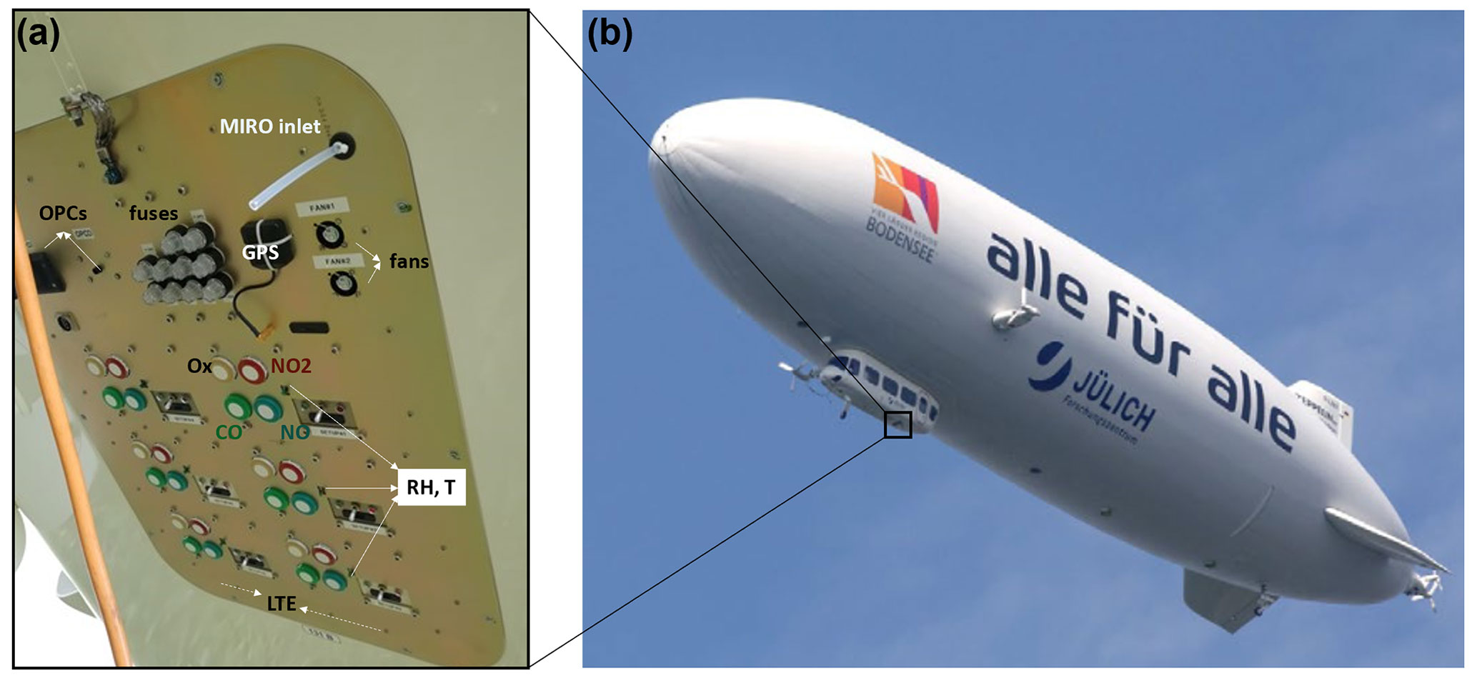
Figure 1 (a) Hatch box, including the sensor setups, located on the bottom of (b) the Zeppelin NT (© Forschungszentrum Jülich/Ralf-Uwe Limbach) that was used as the measurement platform in this work. The reference device, MIRO MGA, was installed inside the gondola but with the inlet line right beside the sensor setups, as shown at the top right of panel (a).

Six electrochemical sensor (ECS) setups are installed at the hatch box, together with a GPS module (Adafruit Ultimate GPS), Long-Term Evolution (LTE) – a standard for wireless broadband communication for mobile devices – equipment for remote access, ventilation fans to regulate the hatch box pressure, two optical particle counters, and fuses to protect the electronics. The hatch box dimensions are $\mathrm{738}\times \mathrm{538}\times \mathrm{162}$ (length × width × height in millimeters). The sensor inlets are located outside of the hatch box and exposed to ambient air via diffusion. A sensor setup, as shown in Fig. S1 in the Supplement, consists of four ECS to measure the trace gases CO, NO, NO₂, and O_x (NO₂+O₃), a Telaire ChipCap 2 sensor for temperature and relative humidity measurements, and a self-developed printed circuit board (PCB) for managing and saving the incoming data at a frequency of 1 Hz. Further specifications of the sensors are given in Table 1. The setups are powered by the Zeppelin NT and further supported by two batteries to provide uninterrupted power to the sensors.

Table 1 Specifications of each sensor setup. Note: ppm is parts per million, and ppb is parts per billion.

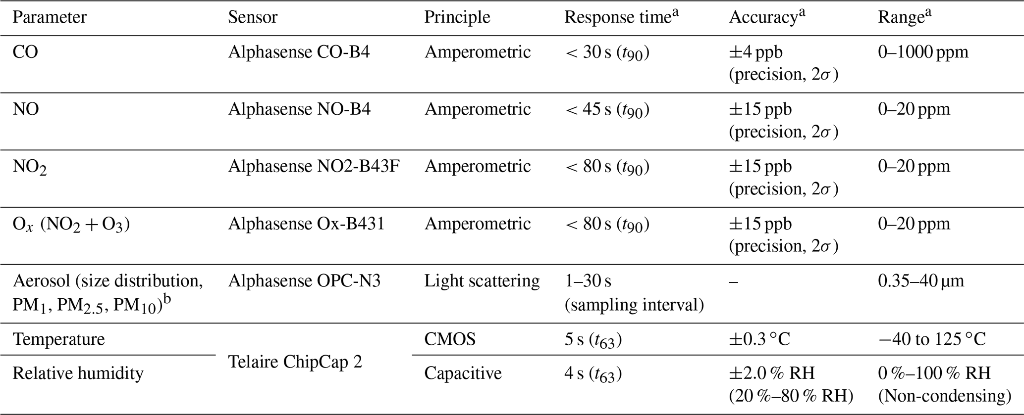
^a Specifications given in the corresponding data sheets. ^b Connected to setup no. 1 and no. 4 but not used in this work.

In this study, we focus on the measurements of NO and NO₂ (NO_x), using electrochemical sensors from Alphasense (Essex, UK). Laboratory evaluation and optimization of the CO and O_x sensor performance is currently ongoing and the focus of a future study, as further discussed in Sect. 2.3.3. Here, the NO_x measurements are performed using amperometric gas sensors that have four electrodes, namely a working electrode (WE), a counter electrode (CE), a reference electrode (RE), and the auxiliary electrode (AUX). The measuring principle is based on a redox reaction that takes place at the WE and the CE (reduction and oxidation). The RE keeps the WE at a constant potential to force the desired electrochemical reaction of the analyte on the three-phase boundary (electrode, electrolyte, and gas). The resulting charges are transferred to each electrode in the form of ions via the electrolyte solution and in the form of electrons via an external circuit. The resulting current of the electron transfer is the measurement signal of the sensor. This current is exactly proportional to the concentration of the analyte when the sensor is operated under appropriate diffusion-limited conditions. Many kinetic factors, such as the mass transfer of the analyte to the electrode and the electrocatalytic activity of the electrode material, can be adjusted via the design of the sensor (Stetter and Li, 2008). AUX has the same design as the WE but is fully immersed in the electrolyte and has no interface with the gas phase (Baron and Saffell, 2017). Therefore, the AUX signal can be used to correct the WE signal from influences on the WE other than the analyte (e.g., temperature). The measured WE and AUX currents are converted into a voltage signal using an individual sensor board (ISB; Alphasense). Finally, this signal is digitized by the measurement board and then recorded on a SD (Secure Digital) card in binary format and can also be transferred serially.

Besides the measurement equipment in the hatch box, a MIRO MGA10-GP multi-compound gas analyzer was installed in the gondola. The MIRO MGA measures the amount fractions of 10 trace gases (NO, NO₂, O₃, SO₂, CO, CO₂, CH₄, H₂O, NH₃, and N₂O) by direct laser absorption spectroscopy. In this study it is used as a reference system for the ECS and enables a direct performance evaluation of the ECS in an airborne setting. Hundt et al. (2018) and Liu et al. (2018) provide more in-depth details about the MIRO, while more information on its use on the Zeppelin NT is given by Tillmann et al. (2022). For an accurate intercomparison to the ECSs, a perfluoroalkoxy alkane (PFA) inlet line with a length of 8 m was placed next to the ECSs in the hatch box (Fig. 1a) and connected to the MIRO. The volumetric flow rate used for the MIRO was 1.2 SLM, resulting in a residence time of the gas inside the line of around 5 s.

2.2 Location and dates

Figure 2a depicts a map with the flight paths for our measurements in 2020. The flights took place within two periods in mid- to late spring, with targeted research flights performed from 29 April to 9 May 2020 and measurements during commercial flights from 27 May to 15 June 2020. All flights were over Germany and predominantly over North Rhine-Westphalia, except for the transfer flights on 29 April and 27 May 2020 from Friedrichshafen to North Rhine-Westphalia and from North Rhine-Westphalia back to Friedrichshafen on 9 May and 15 June 2020. During the targeted flights, specific emission sources, e.g., a power plant, were targeted in addition to cities and rural areas. More detailed information on individual flights is provided by Tillmann et al. (2022). Figure 2b shows the in-flight measured temperature and relative humidity values. According to the manufacturer's specifications, the sensors should be used in the range from −30 to 40 ^∘C and 15 % to 85 % relative humidity (Alphasense, 2019b, a, e, d). Nearly the entire dataset is within these specifications, with 1 % and 99 % percentiles at 8.4 ^∘C (1 %), 25.7 ^∘C (99 %) and 28.0 % RH (1 %) and 84.0 % RH (99 %), respectively. Furthermore, the manufacturer recommendations are given for continuous exposure at high or low RH, which was not observed for the whole dataset, hence limiting the influence of such interferences for this study.

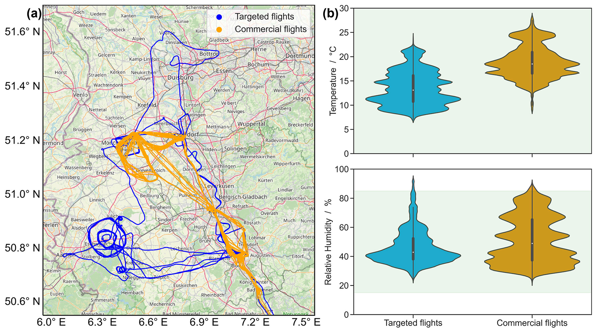
Figure 2 (a) Map with flight paths in North Rhine-Westphalia, Germany (© OpenStreetMap contributors 2021. Distributed under the Open Data Commons Open Database License (ODbL) v1.0), and (b) the frequency distribution of the corresponding temperature and relative humidity in-flight values for the targeted (blue) and commercial (orange) flights, as illustrated in violin plots. The manufacturer-specified limits within which the sensors should be used are depicted in shaded green in the background.

2.3 Data processing

The quality of sensor data can be influenced by various parameters, including transmission errors to the measurement board and electromagnetic interference between the devices (Alphasense, 2013), and defective sensor components. In this work, we use multiple ECSs in parallel to track defective sensors after following the steps that are outlined below.

2.3.1 Time synchronization and noise reduction

The clocks on each of the six sensor setups were manually preset; therefore, time synchronization was not ensured. In the first step, we chose a master setup, here setup no. 2, that was operational throughout all flights with a data coverage of 99 %. Next, a time shift was applied to the other setups to match it. To find the optimal values for this time shift, setup X was shifted from −60 to +60 s, stepwise by 1 s, performing a linear regression analysis (setup $X(t+-x)$ vs. setup no. 2). The linear regression resulting in the highest coefficient of determination, R², was used to correct for the time difference in each setup to the master setup. This was done using the full dataset of each period of flights, both targeted and commercial, resulting in shifts within ±15 s and an average time drift of ±0.31 s per week, leading to a maximum drift of $<\pm \mathrm{1}$ s during each single period of flights.

In the next step, the data of the sensors and the MIRO MGA, whose clock is set via LTE, were synchronized. This synchronization step made it possible to properly compare the sensors with each other and with the reference instrument. Last, to reduce the noise of the ECS signals, a Savitzky–Golay filter (Savitzky and Golay, 1964) was used. Here, a polynomial regression with a window size of 2n+1 adjacent data points is solved by linear least squares. A window of 11 s (n=5) and a polynomial degree of 3 was found to be optimal to smooth the signals without altering the analyte peaks. Figure S3 shows the difference between the sensor signal before and after applying the filter at different NO and NO₂ concentrations. The signal reduction is within 10 ppb (parts per billion; 2σ, corresponding to around 95 % of the data), i.e., similar to the noise levels of the sensors (Fig. S2), independent of the NO and NO₂ concentrations, which highlights the minor influence of the Savitzky–Golay filter on larger peaks.

2.3.2 Temperature and relative humidity data

In addition, six ChipCap 2 sensors were used for temperature and relative humidity measurements. The sensor's measurement principle is based on a capacity change for relative humidity and a resistance variation for temperature. To evaluate the performance of these sensors, we intercompared the differences between the six sensors, as shown in Fig. S4. From these results it is evident that the temperature and relative humidity sensors of setups no. 4, no. 6, and partly no. 5 provide erroneous data. We therefore calculate and use throughout this work the mean values and standard deviations of the remaining, quality-assured temperature and relative humidity measurements, assuming response times within 5 s, as shown in Table 1.

2.3.3 Determination of amount fractions

In this work, we develop a correction method to accurately determine the amount fractions of NO and NO₂ using regression parameters determined with the ECS in-flight data (Sect. 3). A detailed description of the correction procedure is given in the Supplement and is based on the method of Mead et al. (2013). After applying this correction method, the sensor voltage signals in millivolts are converted to amount fractions using sensitivity values in millivolts per part per billion provided by the manufacturer (Table S1 in the Supplement). Here, we assume constant sensitivities, given that their dependency, e.g., to temperature, is a second-order effect (Mead et al., 2013; Popoola et al., 2016).

To account for sensor response times, a low-pass filter, in this case a centered moving average with a window size of 31 s, is used that corresponds to the t₉₀, which is defined as the duration the sensor needs to reach 90 % of the final signal after a step change in concentration. This value is derived from the combined information given by the laboratory measurements (Table S2), which is in agreement with the manufacturer and published measurements (Mead et al., 2013); the manufacturer provides a t₉₀ of <45 s for NO and <80 s for NO₂ from 0 to 2 ppm (parts per million), whereas Mead et al. (2013) provide a t₉₀ of 21 s for NO₂.

As a reference correction method, we use the recommended correction described by the manufacturer (Alphasense, 2019c), following the above equations, to correct the NO and NO₂ WE output for effects of temperature as follows:

$$\begin{array}{}\text{(1)}& {\displaystyle }\begin{array}{rl}{\text{WE}}_{\mathrm{NO},\mathrm{c}}& =\left({\text{WE}}_{\mathrm{u}}-{\text{WE}}_{\mathrm{e}}\right)-k_{\mathrm{T}}\times \left({\displaystyle \frac{{\text{WE}}_{\mathrm{0}}}{{\text{AUX}}_{\mathrm{0}}}}\right)\\ & \times \left({\text{AUX}}_{\mathrm{u}}-{\text{AUX}}_{\mathrm{e}}\right),\end{array}\text{(2)}& {\displaystyle }{\text{WE}}_{{\mathrm{NO}}_{\mathrm{2}},\mathrm{c}}=\left({\text{WE}}_{\mathrm{u}}-{\text{WE}}_{\mathrm{e}}\right)-n_{\mathrm{T}}\times \left({\text{AUX}}_{\mathrm{u}}-{\text{AUX}}_{\mathrm{e}}\right),\end{array}$$

where WE and AUX are the working and auxiliary electrode voltages. The subscripts u, e and 0 stand for the uncorrected components, i.e., measured signal, the electronic offset, and the sensor zero, respectively. The electronic offsets and sensor zero values are provided by the manufacturer and given in Table S1. WE_NO,c and WE${}_{{\mathrm{NO}}_{\mathrm{2}},\mathrm{c}}$ are the corrected working electrode voltages for NO and NO₂, respectively. The temperature compensation factors k_T and n_T are given in the range of −30 to 50 ^∘C in 10 ^∘C steps. For temperatures within these 10 ^∘C steps, a linear interpolation is advised.

ECSs were also used to measure CO and O_x (NO₂+O₃). A comparison of the ECS measurements to the MIRO reference instrument was performed after following the manufacturer's recommendations to estimate amount fractions for CO and O_x. However, high uncertainties were found due to the high CO and O₃ backgrounds creating an offset to the sensors that was not accurately accounted for based on the manufacturer's correction procedure (Fig. S5). Additionally, the described correction procedure in the Supplement that is used in this work for NO and NO₂ relies on periods with low analyte concentrations, ideally at zero, to account for offsets of the background signal. While this is a good approximation for NO and NO₂, it is not applicable to CO and O₃ because of their higher background concentrations which are often above several tens of ppb. Laboratory evaluation and optimization of the CO and O_x sensor performance is currently ongoing and the focus of a future study. In this work, we evaluate the performance and highlight the potential of the NO and NO₂ sensors for accurate airborne applications.

3 Results and discussion

3.1 Sensor signal dependencies

All Zeppelin measurements were filtered for periods of low NO and NO₂ concentrations (<2 ppb) using the measurement data of the reference instrument in order to find possible interferences in the WE signal of the electrochemical sensors. This procedure reduces the data to only background concentration periods and provides the signal that is influenced by cross-interferences. The correction method developed and described in the following is entirely independent of a reference device and requires only the sensors used. Figures 3 and S6 show the correlation of WE to AUX, T, and $\mathrm{d}\text{RH}/\mathrm{d}t$ at different time resolutions (i.e., averaging intervals) for NO and NO₂, respectively. For 1 s resolution, coefficients of determination (R²) are 0.86, 0.71, and 0.83 for NO and 0.57, 0.13, and 0.86 for NO₂ with respect to AUX, T, and $\mathrm{d}\text{RH}/\mathrm{d}t$, respectively. For this dataset, we could not detect any other significant dependencies, including $\mathrm{d}T/\mathrm{d}t$ (Fig. S7). As described in Sect. 2.1, AUX can be used to correct the WE signal from external interferences. The collinearity between AUX and T that is shown by the colored dataset in Fig. 3 further promotes the significant influence of temperature on the sensor measurements. However, other unknown interferences could have a simultaneous effect on WE and AUX, such as changes in the electrolyte composition or influences on the sensor board electronics that control the voltages of the electrodes. Therefore, we also consider AUX to be an additional correction parameter, despite the observed collinearity with temperature.

Figure 3 shows that temperature and AUX dependencies are effective on a longer timescale, since the relationship with WE does not change with lower time resolutions transitioning from 1 to 30 and 120 s. On the contrary, the correlation with $\mathrm{d}\text{RH}/\mathrm{d}t$ decreases progressively with decreasing time resolution. Since ECSs are mostly deployed for long-term monitoring of air quality at, for example, stationary monitoring stations, mean values of up to 1 h are often used (Mijling et al., 2018). Therefore, at longer time resolutions, such effects are filtered out. However, for mobile applications, a high time resolution results in a better spatial resolution of the pollutant distributions, making this effect relevant.

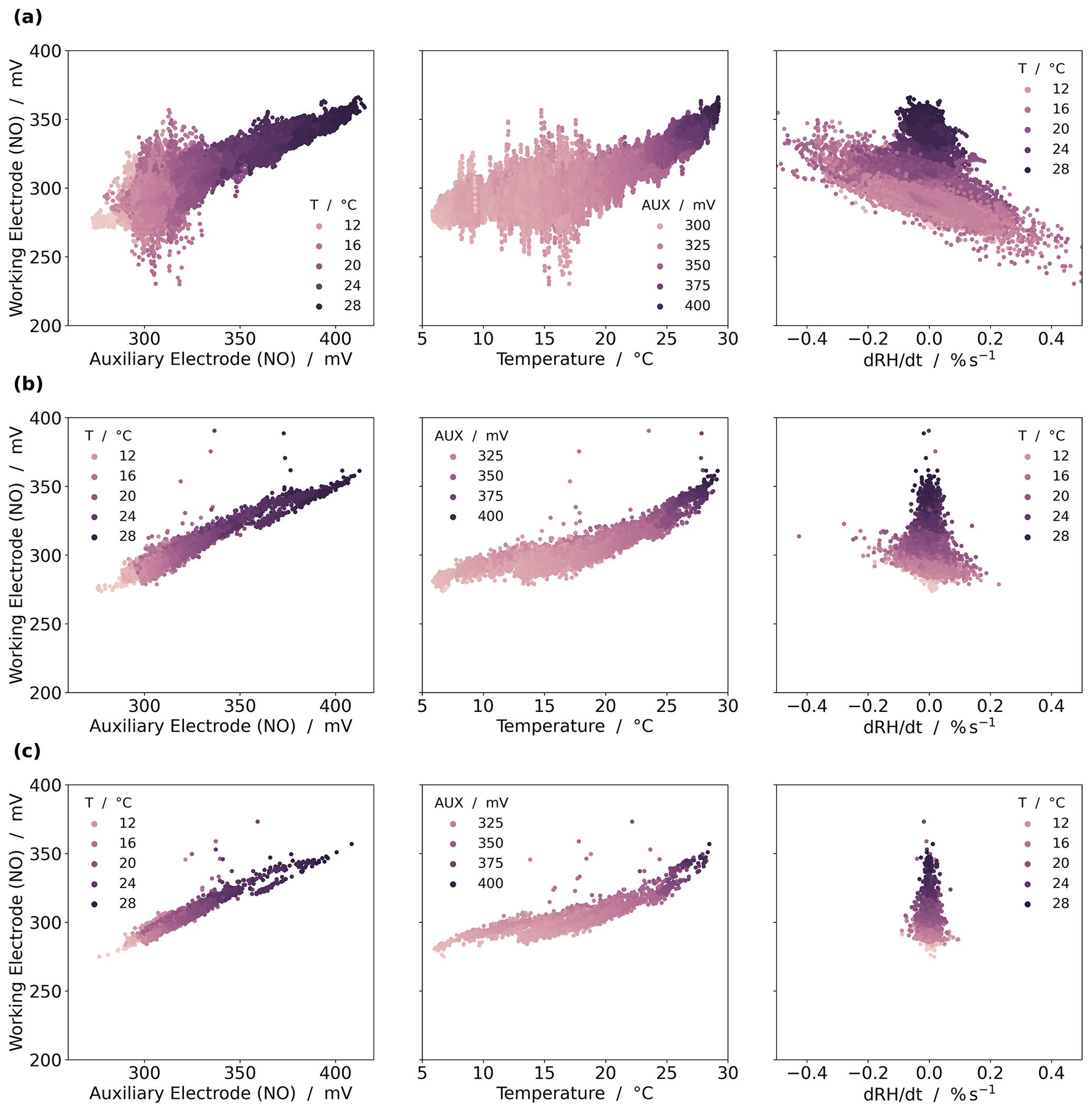
Figure 3 Scatterplots of NO sensor (setup no. 2) for WE vs. AUX, T, and $\mathrm{d}\text{RH}/\mathrm{d}t$, with different time resolutions of (a) 1 s, (b) 30 s, and (c) 120 s provided per row. The colors are used to show collinearity between AUX and T and that the shift in WE voltages in the $\mathrm{d}\text{RH}/\mathrm{d}t$ plot is a temperature interference.

Previous publications have shown the influence of humidity changes on the WE signal, after which there is a spike in the signal followed by a slow decay (Mueller et al., 2017; Pang et al., 2017, 2018). Mueller et al. (2017) conducted laboratory tests with relative humidity changes of 5 % RH every 20 min between 40 % RH and 60 % RH. They observed that this changed the sensor signal by a similar order of magnitude to the addition of 70 ppb NO₂. Afterwards, the signal decreased exponentially in time back to equilibrium. Through further measurements, they found that the effect was dependent on the magnitude and rate of the relative humidity variation that can affect the measurement accuracy over minutes to hours – but the physical reason for this is currently unknown. Pang et al. (2017) came to a similar conclusion. Rapid RH changes (≈20 % min⁻¹) had an immediate influence on the sensor signal, followed by a required recovery period of up to 40 min to restore the original value, whereas small humidity changes of about 0.1 % min⁻¹ had no significant effect. When compared to our measurements, the humidity changes in these laboratory experiments are unidirectional and over a longer timescale. During the flights, we observe both negative and positive humidity changes on a short timescale. For example, the mentioned 20 % min⁻¹ RH change that triggers the long recovery phase results in 0.33 % s⁻¹, assuming a linear increase. During the Zeppelin flights, we observe such a longer-lasting effect, starting at about 0.7 % s⁻¹, after which it takes up to 5 min for the signal to stabilize again, depending on the magnitude of the rate of change. Since we do not have an exact analytical solution for correcting this dependency yet, these values were removed from the dataset. However, we were able to describe the dependence of the WE voltages on the temporally small-scale changes in relative humidity (max ±0.6 % s⁻¹), which affect the signals only immediately and briefly, with a linear relationship (see Fig. 3).

In the following, we use the above correlations on T, AUX, and $\mathrm{d}\text{RH}/\mathrm{d}t$ to develop a correction method using the equations below for NO and NO₂.

$$\begin{array}{}\text{(3)}& \begin{array}{rl}{\text{WE}}_{\mathrm{NO},\mathrm{c}}\left(t\right)& ={\text{WE}}_{\mathrm{NO},\mathrm{a}}\left(t\right)-{\mathit{\beta }}_{\mathrm{0}}\times {\displaystyle \frac{\mathrm{d}\text{RH}}{\mathrm{d}t}}\left(t\right)\\ & -\left(\mathit{\alpha }+{\mathit{\beta }}_{\mathrm{1}}\times \exp \left({\mathit{\beta }}_{\mathrm{2}}\times T\left(t\right)\right)+{\mathit{\beta }}_{\mathrm{3}}\times \text{AUX}\left(t\right)\right),\end{array}\end{array}$$

$$\begin{array}{}\text{(4)}& \begin{array}{rl}{\text{WE}}_{{\mathrm{NO}}_{\mathrm{2}},\mathrm{c}}\left(t\right)& ={\text{WE}}_{{\mathrm{NO}}_{\mathrm{2}},\mathrm{a}}\left(t\right)-{\mathit{\beta }}_{\mathrm{0}}\times {\displaystyle \frac{\mathrm{d}\text{RH}}{\mathrm{d}t}}\left(t\right)\\ & -\left(\mathit{\alpha }+{\mathit{\beta }}_{\mathrm{1}}\times T\left(t\right)+{\mathit{\beta }}_{\mathrm{2}}\times \text{AUX}\left(t\right)\right),\end{array}\end{array}$$

where WE_a is the WE signal after the preparation steps from Sect. 2.3.1, T is the temperature in degrees Celsius, and α, β_z (z= 0, 1, 2, 3) are the determined regression parameters. We give a more detailed description of how to obtain Eqs. (S3) and (S4) in the Supplement and show the regression parameters in Table S3. To calculate the amount fractions, WE_NO,c and WE${}_{{\mathrm{NO}}_{\mathrm{2}},\mathrm{c}}$ are then divided by the corresponding sensitivities of the sensors (Table S1). In the following sections, we will often use NO_x (NO+NO₂). For the ECSs, this means the following:

$$\begin{array}{}\text{(5)}& x_{{\mathrm{NO}}_x}\left(t\right)={\displaystyle \frac{{\text{WE}}_{\mathrm{NO},\mathrm{c}}\left(t\right)}{S_{\mathrm{NO}}}}+{\displaystyle \frac{{\text{WE}}_{{\mathrm{NO}}_{\mathrm{2}},\mathrm{c}}\left(t\right)}{S_{{\mathrm{NO}}_{\mathrm{2}}}}},\end{array}$$

in which the summands are moving averages, as described in Sect. 2.3.3, to consider the response time of the ECSs.

3.2 Validation of ECSs performance

3.2.1 Intercomparison of ECS setups

Table 2 shows the intercomparison of all ECS setups, after applying the corrections presented in Sect. 3.1, by performing linear regression analysis including their slopes, the intercepts, and coefficients of determination R². All NO sensors are in good agreement with slopes ranging from 0.92 to 1.12, intercepts from ±0.09 to ±5.91 ppb, and R²>0.99, whereas for NO₂ slopes range from 0.82 to 1.07, intercepts from ±0.07 to ±4.29 ppb, and R² from 0.80 to 0.94. Although the R² is high for all setups, the regressions of setup nos. 4 and 5 with the NO sensors show greater variability in terms of intercepts and slopes. For NO, setup no. 5 has the highest offset of 5.91 ppb and a larger slope compared to all other setups. For NO₂, the results are not as definite, but the R² is generally lower for setup nos. 4 and 5, indicating the higher noise of the sensors. This is also further supported by Fig. S8, with the noise of the sensor setup nos. 4 and 5 at 5.03 and 3.59 ppb for NO and 6.32 and 5.43 ppb for NO₂, respectively. Setup nos. 3 and 6 have similar precisions for NO compared to setup no. 2, with values of 1.45 and 1.98 ppb compared to 1.95 ppb, respectively; however, their noise for NO₂ is approximately 55 % and 61 % higher than for setup no. 2. Therefore, we exclusively use setup no. 2 in the following, given the consistent agreement to other sensors, the lower noise, and the high in-flight data coverage >98 %.

Table 2 From left to right are the (a) slopes, (b) intercepts, and (c) R² of the linear regressions between one setup and any other setup for ≈286 h of measurements (≈75 h in flight). The lower triangles, depicted with black framed rectangles, are the NO sensors results. The gray diagonally striped rectangles in the upper triangle show the results of the NO₂ sensors. The light-to-dark color map indicates the range from worst to best values, respectively.

The regression parameters for NO₂ are more variable than for NO. One possible reason is the smaller temperature dependence for NO₂. As a result, AUX, for example, for setup no. 2, varies only between 220 and 240 mV, whereas NO varies between 300 and 400 mV (Figs. 3 and S6). This indicates that the temperature influence is the dominant contribution for the baseline correction of the NO sensor, whereas the WE of the NO₂ sensor could additionally be influenced by other interfering factors that do not affect the AUX and are not accounted for here. Another factor is the much larger number of data points for NO (n=4026) than for NO₂ (n=155) for amount fractions above 50 ppb, leading to a more stable regression line for NO.

3.2.2 Noise reduction

Figure 4 shows the distributions of the standard deviations of the NO (Fig. 4a) and NO₂ (Fig. 4b) sensors for each of the 31 s windows, which were used to calculate the moving average (Sect. 2.3.3). The data were filtered for periods with height above 100 m (n=270 198) to avoid engine exhaust peaks that would result in high standard deviations because of the high changes in concentrations inside these time windows. The correction used here, shown in blue and green, results in the lowest noise, with modal values for NO of 2.03 ppb for the correction with T and AUX and 1.95 ppb when $\mathrm{d}\text{RH}/\mathrm{d}t$ is additionally included in the correction, whereas for NO₂, the noise modal values are 3.66 and 3.32 ppb. Besides the change in peak position, the distributions become narrower when correcting with $\mathrm{d}\text{RH}/\mathrm{d}t$. This leads to significantly higher peaks of around 60 % for both analytes because the number of data points with standard deviations above 3 ppb for NO and above 5 ppb for NO₂ decreases, highlighting the significant noise reduction when including $\mathrm{d}\text{RH}/\mathrm{d}t$ in the correction procedure.

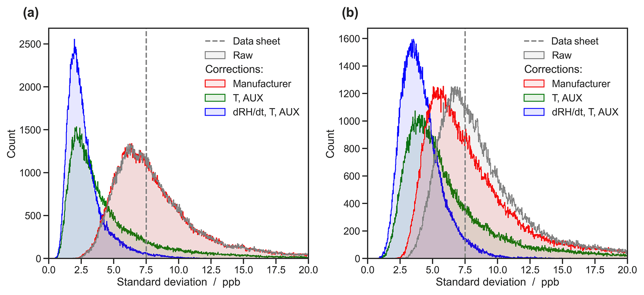
Figure 4 Distributions of standard deviations calculated inside 31 s windows shown for (a) NO and (b) NO₂ sensors of setup no. 2 and filtered for flights above 100 m to avoid engine exhaust peaks (number of data points =270 198). Adding $\mathrm{d}\text{RH}/\mathrm{d}t$ to the correction procedure leads to a narrower distribution by reducing high changes in the signal on a short timescale.

3.2.3 Comparison of ECSs with the MIRO MGA

Figure 5a and b show the amount fractions of NO_x for sensor setup no. 2 (master setup; see Sect. 2.3.1), following the corrections recommended by the manufacturer, as described in Sect. 2.3.3, whereas Fig. 5c and d show the correction method developed in this work compared to the MIRO MGA used as a reference device. Additionally, comparisons of all setups with the MIRO MGA are shown in Fig. S10. As shown in Fig. 5a and c, the deviations of the sensor values to MIRO decreased from an absolute average of 27.3±4.8 to 3.5±3.1 ppb. This means an absolute accuracy improvement by nearly an order of magnitude. The accuracy increase is mainly the result of the improved offsets changing from −13.15, −8.29, and −19.76 to 9.12, −6.76, and 3.15 ppb for NO, NO₂ (Fig. S9), and NO_x, respectively. Precision also improved, as reflected by the decrease in the associated error bars in Fig. 5, resulting in a higher coefficient of determination from 0.54 to 0.88. In general, NO and NO₂ measurements corrected with our method, and the resulting NO_x values are close to the 1:1 line. Moreover, the 2 standard deviations corresponding to 95 % of the data in each bin are within a factor of 2 above 20 ppb, which is particularly driven by the $\mathrm{d}\text{RH}/\mathrm{d}t$ correction, as also shown in Fig. 4.

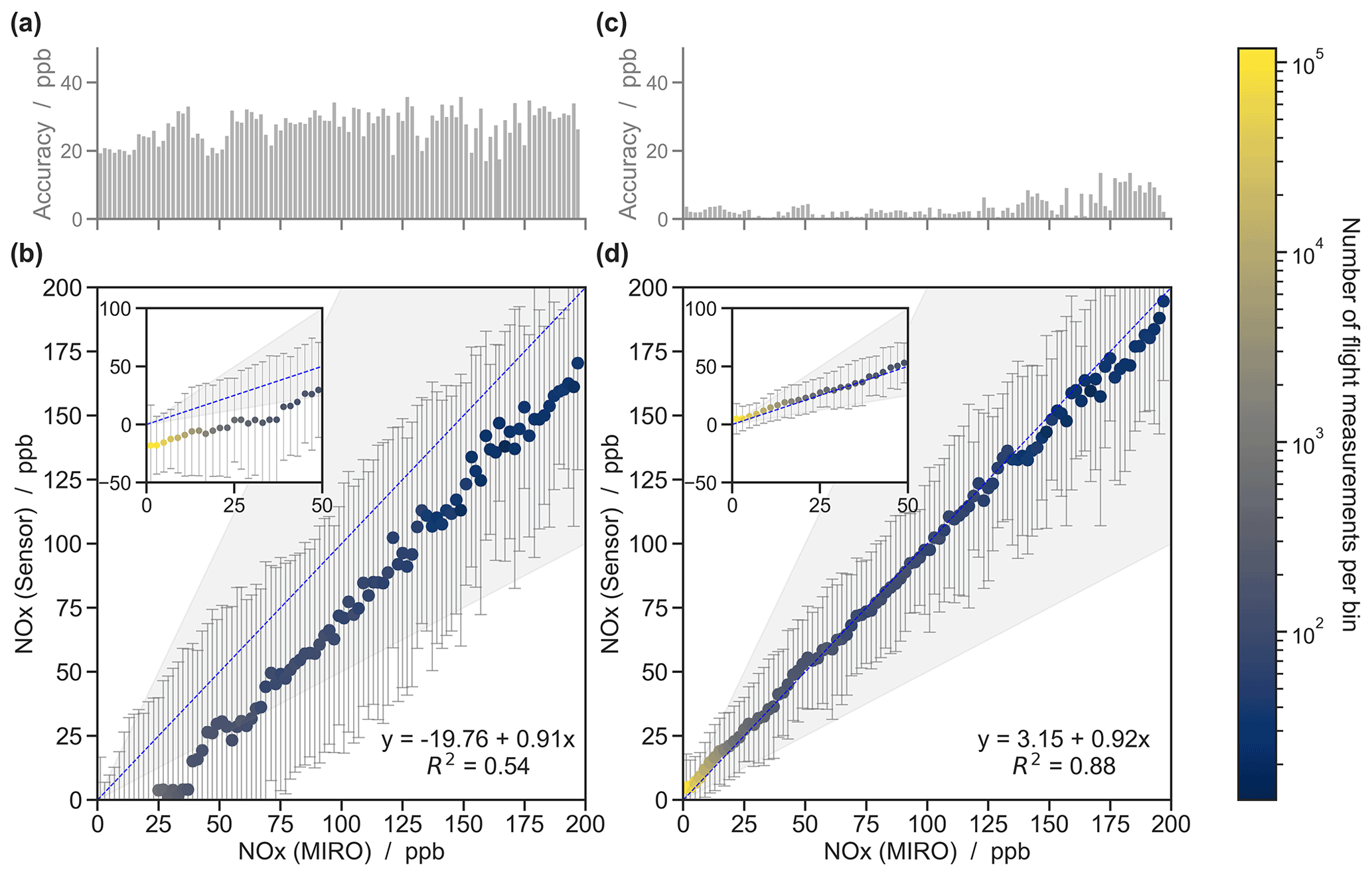
Figure 5 Scatterplots of the in-flight-corrected (≈75 h) NO_x sensor data (setup no. 2) vs. MIRO MGA data (reference) classified in 2 ppb bins and 2 times the standard deviations (±2σ). Shown in panels (a) and (c) are the accuracies for each bin, i.e., the absolute difference between sensor and MIRO MGA data per bin. Panels (a) and (b) represent the corrections, as recommended by the manufacturer, whereas panels (c) and (d) provide the results of our correction method. The dashed blue line marks the 1:1 line, and the range of 2:1 and 1:2 is shaded in gray. The inlet plots show the data in a higher resolution from 0 to 50 ppb of the reference instrument. In addition, the linear regression results are shown at the bottom right.

While, on average, there is agreement within 3.5 ppb for NO_x between the MIRO and ECSs at both high and low concentrations, this agreement is not evident for the lower amount fractions of NO or NO₂ (Fig. S9). For NO, an average overestimation of 34.4 % is observed below 40 ppb that increases to an average deviation of up to 600 % in the range of 0 to 5 ppb, whereas for NO₂ an underestimation of 31.3 % is observed for amount fractions below 25 ppb, increasing to 300 % below 5 ppb, because of the small absolute numbers. It is possible that the 8 m sampling line to the MIRO could influence the composition of NO and NO₂, as an in-line reaction of NO with O₃ could lead to higher NO₂ and lower NO concentrations, compared to the sensors that have no sampling line. However, this effect is expected to be minor due to the short sample residence time of 5 s. In addition, other parameters may influence the performance of the electrochemical sensors compared to the MIRO, such as cross-sensitivities to other gases, the wind speed (Mead et al., 2013), or the atmospheric pressure. In this study, measurements of gases are limited to CO, CO₂, CH₄, N₂O, H₂O, and O₃ that are performed by the MIRO MGA (Tillmann et al., 2022). No significant cross-interference was observed under the present atmospheric concentrations, as shown in Fig. S12. To quantify possible influences from wind speed and atmospheric pressure, a measuring chamber of a constant volumetric flow, together with pressure sensors, will be used in future campaigns.

Besides the above direct influences, there is also the possibility of sensor drifts, i.e., a change in the sensor signal with time. Wei et al. (2018) estimated a possible drift of <2 ppb per month, whereas Mead et al. (2013) state that the sensitivity of the sensors remained unchanged over an 11-month measurement period. For our deployment duration of 1.5 months, sensor drifts are therefore expected to be within the uncertainty in the measurements, which is also reflected by the good agreement of the ECS and the MIRO in Figs. 5 and S10. Furthermore, Fig. S11 shows the time series of all sensors during different flight days in May and June to evaluate the influence of such sensor drifts. The consistent correlation of all setups to the MIRO highlights the stability of the sensors during this study. However, we promote the need for controlled laboratory measurements in the future to evaluate long-term influences on the stability of the ECS signals, including sensor drifts.

Evidently, with the manufacturer's correction, amount fractions (Fig. 5 a) cannot be accurately quantified predominantly due to the high offset of −19.76 ppb. One possible reason is that, in Eqs. (1) and (2), the same temperature compensation factors are used for all sensors, whereas each sensor may react differently to a temperature change, which is also shown by our regression parameters in Table S3. Another cause could be a drift of the zero value, which is not caught by the temperature and AUX correction in these equations. In our method, sensor drifts are corrected by using minimum values of measured WE voltages, following the procedure described in Mead et al. (2013), as discussed in Sect. 2.3 and the Supplement.

3.3 Detection of anthropogenic NO_x emission sources

After the successful validity check by comparing the corrected sensor data with the reference device in the former section, we now present possible applications and the potential of ECSs for airborne measurements. Figure 6a and b show the flight path on 6 May 2020 between 07:30 and 08:30 UTC in Eschweiler, North Rhine-Westphalia, Germany, when using the reference instrument and the ECSs, respectively. Another example is shown in Fig. 6c and d during a Zeppelin flight over Duisburg-Nord (Hamborn), North Rhine-Westphalia, Germany, on 7 May 2020 between 13:30 and 14:15 UTC. As depicted in Fig. 6a, NO_x background concentrations are 4.9±2.0 ppb and increase significantly in the northwest to a maximum of 21.3±2.2 ppb due to the emissions from the lignite-fired power plant located near the flight path (Tillmann et al., 2022), which is further supported by the wind data that were extracted from high-resolution model simulations. When applying the correction method recommended by the manufacturer for the ECSs (Sect. 2.3.3), background concentrations of NO_x are at $-\mathrm{8.6}\pm \mathrm{5.2}$ ppb and the industrial plume emissions at 11.3±17.3 ppb, highlighting the limitations of this method. However, after applying the correction method developed in this work, as shown in Fig. 6b, a significant improvement is observed, with background concentrations at 3.5±4.2 ppb and the power plant plume average at 21.4±6.6 ppb (Fig. S13a). This results in 40 % higher background concentrations for the sensor measurements in comparison to the MIRO and 5 % lower concentrations for the in-plume measurements.

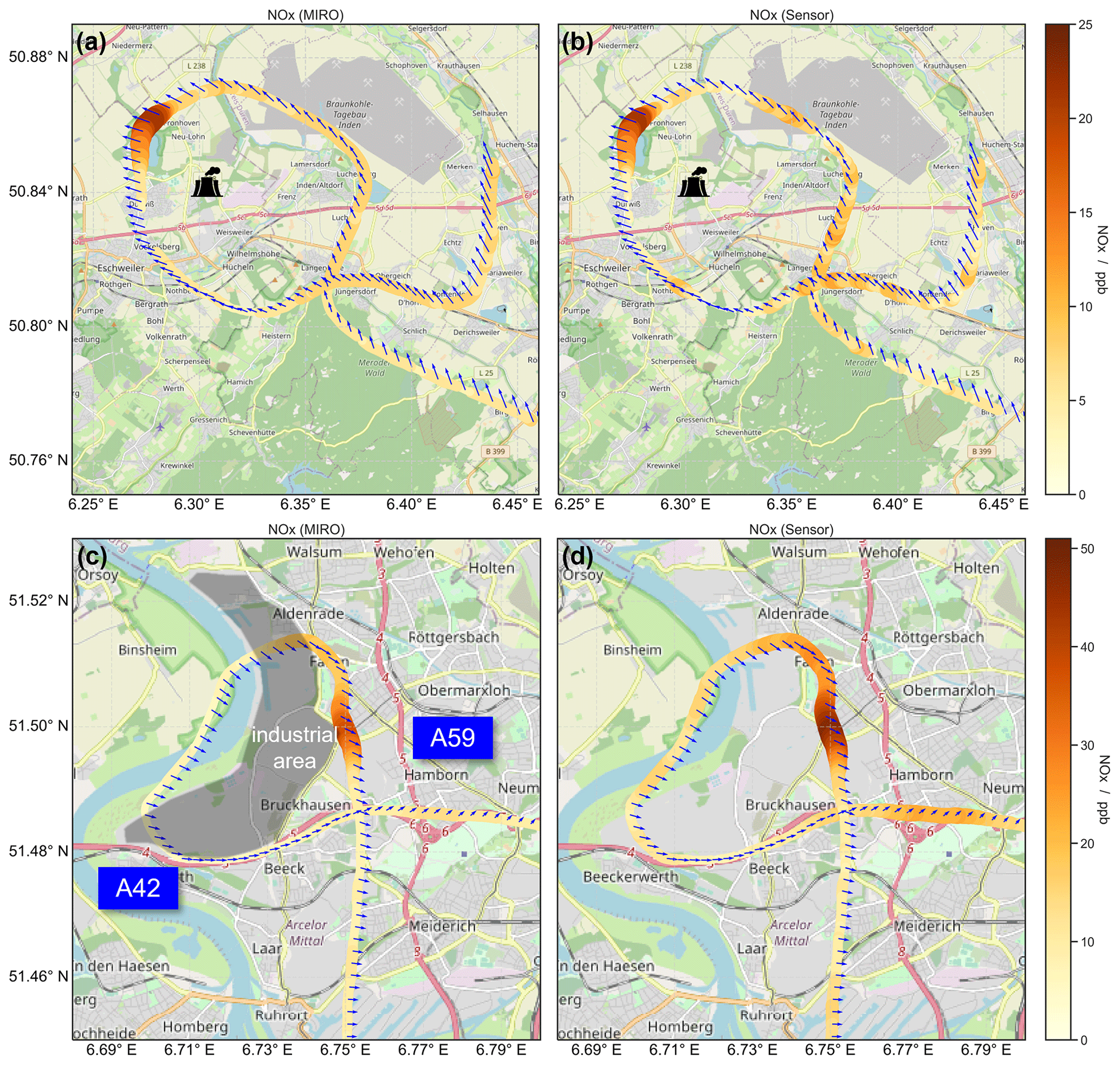
Figure 6 Amount fractions of NO_x are shown by color and size for the MIRO MGA (a, c) and the corrected sensor data of setup no. 2 (b, d) during flights in North Rhine-Westphalia, Germany, near and in the cities of Eschweiler and Duisburg, respectively (© OpenStreetMap contributors 2022. Distributed under the Open Data Commons Open Database License (ODbL) v1.0). The orientation and length of the arrow indicate the wind direction and wind speed (2.1 to 7.2 m s⁻¹ for panels a and b and 1.0 to 2.6 m s⁻¹ for panels c and d; data from EURAD-IM, WRF), respectively. With this, the emission sources can be narrowed down to a lignite-fired power plant located southeast of the detected peak (a, b) and to a steel industry (c, d) located in the gray shaded area.

Similar results can be seen in Fig. 6c and d. Duisburg is known for its industry; there is a steel mill in this district, which is supplied with electricity by the gas-fired combined heat and power plant located on site. In addition, the motorways A42 and A59 run through the area. Westerly winds indicate that the source of emissions during the observed maximum amount fractions of 37.7±6.1 ppb for the MIRO and 47.1±6.4 ppb (Fig. S13b) for the sensor measurements are from the steel mill and the heat and power plant. The influence of highway emissions on the NO_x concentrations is observed at around 51.48^∘ N and 6.77^∘ E when southerly wind directions transported emissions from the A42 and A59 highways to our sampling line. This is especially evident not only for the sensor data (Fig. S13d) but also observable for the MIRO (Fig. S13c). Here, the peak values are 13.8±0.7 and 22.6±3.6 ppb for the MIRO and the ECS, respectively.

These case examples highlight the potential of the ECSs to detect emission sources with concentrations down to 20 ppb. Although, there are larger relative uncertainties due to the deviations in the individual NO and NO₂ sensors (see Sect. 3), the ECSs show better agreement with the MIRO at higher concentrations, especially for NO_x, further promoting their potential for airborne applications.

4 Conclusions

We showed that electrochemical sensors (ECSs) can be successfully used for airborne in situ measurements in the PBL. For this, we used a Zeppelin NT to perform an in-flight comparison of six sensor setups with a reference device during two measurement campaigns, including targeted and commercial flights, in Germany from April to June 2020. Each setup consisted of four electrochemical sensors for CO, NO, NO₂, and O_x (NO₂+O₃) and one sensor each for temperature and relative humidity. These were installed in a custom-built hatch box mounted under the gondola. A quantum cascade laser-based multi-compound gas analyzer, called MIRO MGA, was placed as a reference instrument inside the gondola with an inlet line beside the ECSs.

We developed a standalone correction method, i.e., independent of a reference device, for the ECSs that accounts for external influences on the NO and NO₂ sensor signals by using the variability in the auxiliary electrode voltage, temperature, and the relative humidity gradient. We show that this correction method substantially improves the accuracy down to 6.3±5.7 and 8.7±5.9 ppb and lowers the noise (1σ) of the ECS to 1.92 and 3.32 ppb for NO and NO₂, respectively. The combination of both sensor types (NO and NO₂) leads to a further improved accuracy of 3.5±3.1 ppb for NO_x. When compared to the MIRO MGA, good agreement with a coefficient of determination of 0.88 and a slope of 0.92 is achieved for NO_x measurements. However, at lower concentrations below 40 and 25 ppb, average deviations of 34.4 % and −31.3 % for NO and NO₂, respectively, were evident. Below 5 ppb, these deviations increased up to 300 % and −600 %, because of the small absolute values, indicating the limitations of ECSs for accurate quantification at lower amount fractions.

We highlight the potential to use the sensors for emission source identification during Zeppelin flights by identifying emissions from a lignite-fired power plant with a peak of approximately 21 ppb of NO_x and from a large industrial area in Duisburg with a peak above 40 ppb.

Results from this work emphasize the potential of these sensors for in situ airborne applications and provide a first milestone for future quality-assured use on board UAVs without the need for a reference device. A comprehensive characterization in the laboratory, including the simulation of airborne conditions, before and after such applications, will improve the ECS data quality even further.