Retrieval of snow layer and melt pond properties on Arctic sea ice from airborne imaging spectrometer observations

A melting snow layer on Arctic sea ice, as a composition of ice, liquid water, and air, supplies meltwater that may trigger the formation of melt ponds. As a result, surface reflection properties are altered during the melting season and thereby may change the surface energy budget. To study these processes, sea ice surface reflection properties were derived from airborne measurements using imaging spectrometers. The data were collected over the closed and marginal Arctic sea ice zone north of Svalbard in May–June 2017. A retrieval approach based on different absorption indices of pure ice and liquid water in the near-infrared spectral range was applied to the campaign data. The technique enabled us to retrieve the spatial distribution of the liquid water fraction of a snow layer and the effective radius of snow grains. For observations from three research flights, liquid water fractions between 6.5 % and 17.3 % and snow grain sizes between 129 and 414 µm were derived. In addition, the melt pond depth was retrieved based on an existing approach that isolates the dependence of a melt pond reflection spectrum on the pond depth by eliminating the reflection contribution of the pond ice bottom. The application of the approach to several case studies revealed a high variability of melt pond depth, with maximum depths of 0.33 m. The results were discussed considering uncertainties arising from the airborne reflection measurements, the setup of radiative transfer simulations, and the retrieval method itself. Overall, the presented retrieval methods show the potential and the limitations of airborne measurements with imaging spectrometers to map the transition phase of the Arctic sea ice surface, examining the snow layer composition and melt pond depth.

1 Introduction

Compared to the whole globe, the Arctic experiences an enhanced warming, which is referred to as Arctic amplification (Serreze and Francis, 2006; Serreze and Barry, 2011). The surface albedo feedback is one of the most important mechanisms driving Arctic amplification (Curry et al., 1995; Hall, 2004; Pithan and Mauritsen, 2014; Wendisch et al., 2023). The Arctic sea ice albedo depends on wavelength, solar zenith angle, snow grain size, and shape as well as snow layer morphology, impurities, and liquid water fraction. Therefore, the sea ice albedo is strongly altered by melting processes (Warren, 1982; Kokhanovsky and Zege, 2004; Dozier et al., 2009; Gardner and Sharp, 2010).

Following the snow metamorphism, the deposited snow grains become more spherical and larger, leading to a decrease of surface albedo (Warren, 1982; Colbeck, 1983; Gubler, 1985). During the summer months, the initially dry and cold snow layer covering the sea ice surface is beginning to melt, thereby undergoing three melting stages: moistening, ripening, and runoff (Dingman, 2015). Meltwater accumulates in the initially air-filled interstices between the snow grains, leading to a further surface albedo decrease. In this stage, the melting snow layer is composed of a mixture of ice, liquid water, and air, as schematically illustrated in Fig. 1 (I. Snow melting). If the maximum snow grain interstitial capacity is reached, the runoff phase begins (Dingman, 2015). Meltwater accrues in sea ice surface depressions and melt ponds form (Polashenski et al., 2012), as illustrated in Fig. 1 (II. Ponding). The meltwater volumes stored in melt ponds, depending on surface area and depth, represent a significant portion of the ice surface meltwater balance (Perovich et al., 2021). Overall, Fig. 1 demonstrates the sea ice surface transition from a melting snow layer to the beginning of melt pond formation in late spring and early summer, which is characterized by a distinct surface albedo decrease (Perovich and Polashenski, 2012). To observe this phase in more detail, the snow grain size, snow layer wetness, and melt pond depth are important parameters characterizing the melting processes. Past Arctic field campaigns provided in situ surface albedo measurements over a melting snow layer and melt ponds (Perovich et al., 2002; Light et al., 2022). The retrieval of the regarded properties was already the subject of several studies. Bohn et al. (2021) developed a methodology to retrieve snow grain size, liquid water fraction, and the mass mixing ratio of light absorbing particles from spectral reflection measurements with optimal estimation for airborne and spaceborne applications. Jäkel et al. (2021) compared optical-equivalent snow grain radius retrieval methods based on the grain-size-dependent absorption in the solar spectral range, which were applied to ground-based, airborne, and spaceborne reflection measurements. Grain sizes below 300 µm were retrieved for springtime snow layers on sea ice. Hannula and Pulliainen (2019) examined the snow reflection in visible to near-infrared spectral bands as a function of wetness in a laboratory experiment. Marin et al. (2020) investigated the information on snow wetness in spaceborne radar observations.

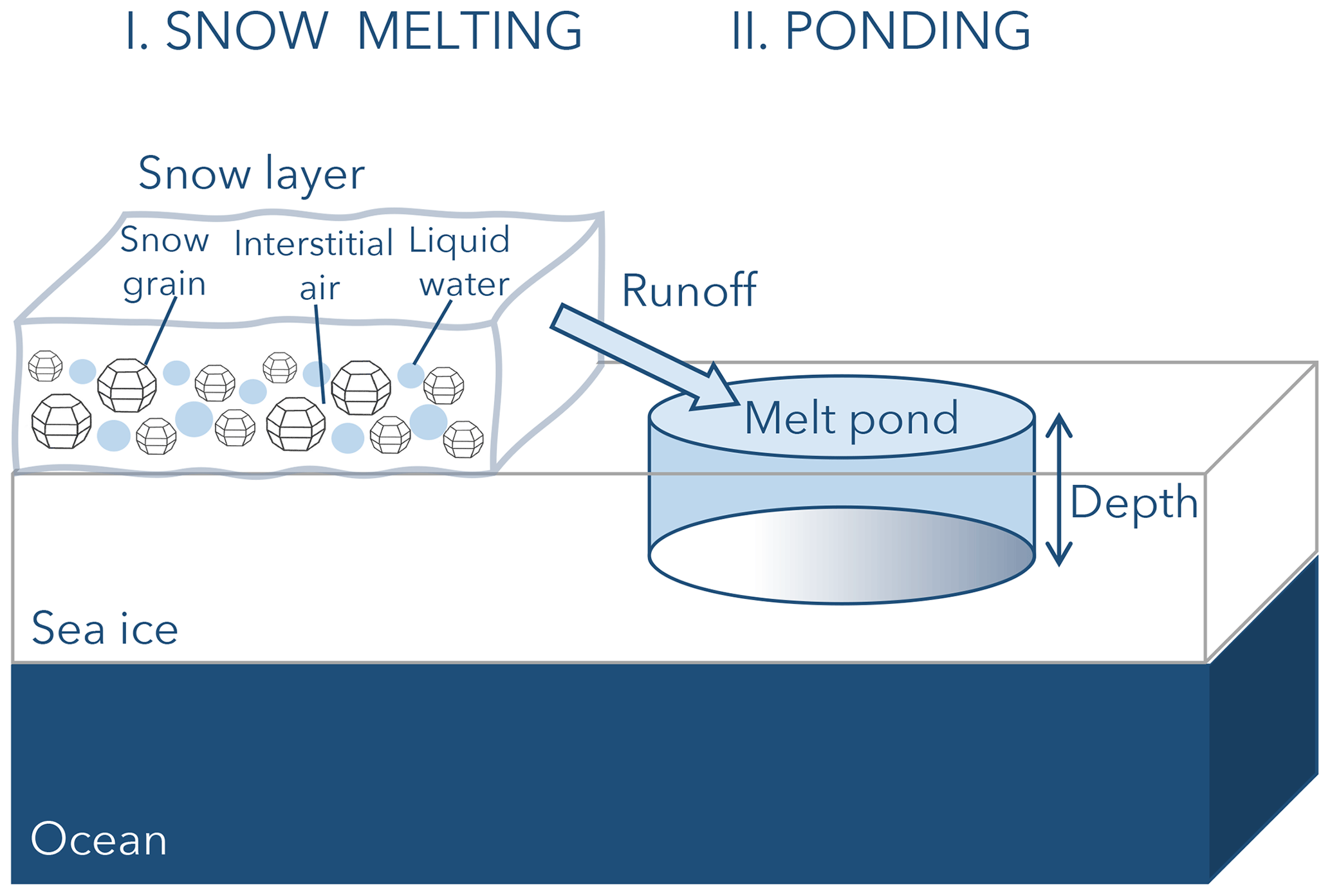
Figure 1 Schematic overview of the sea ice surface transition during the early melting season: a melting snow layer (I.) as a composition of snow grains, liquid water, and interstitial air, determining the ongoing albedo decrease. With start of the runoff phase, the melt pond formation (II.) is induced. The reflective behavior of the melt pond is described by its depth and the ice bottom albedo, indicated by a color gradient.

To quantify the snow layer wetness, the liquid water fraction f_LW is a useful measure. It is defined as the ratio of snow layer liquid water content (LWC) and total water content (TWC = ice water content + LWC), which are both given in units of grams per cubic meter (g m⁻³). Therefore, the f_LW of a snow layer can range between 0 % (dry snow) and 15 % (very wet snow), reaching a soaked state with f_LW>15 % (Fierz et al., 2009). A snow reflection spectrum is sensitive to the snow layer wetness in the near-infrared spectral range because of different absorption characteristics of liquid water and pure ice (Warren, 1982; Kou et al., 1993). Based on the spectral dependence of local absorption minima and maxima, Green et al. (2002) retrieved snow layer liquid water fraction and snow grain size by comparing measured snow reflection spectra with simulations for varying snow grain sizes and liquid water fractions. This approach was tested on a snow sample block in the field under cloud-free solar illumination by Green et al. (2002) and validated by Donahue et al. (2022) with further field and laboratory experiments.

The reflection of melt ponds depends on the melt pond ice bottom reflection and pond depth (Malinka et al., 2018). Based on this dependence, several approaches retrieving the pond depth were developed (Legleiter et al., 2014; Malinka et al., 2018; Lu et al., 2018). König and Oppelt (2020) derived a linear model to isolate the dependence of the pond reflection spectrum on the pond depth. Typically, the depth of melt ponds on sea ice reaches at maximum 1 m and is dependent on the local meltwater availability and surface topography. Multi-year ice is usually characterized by surface ridges and depressions providing vertically more extended basins for deeper melt ponds compared to often level first-year ice surfaces, on which shallower ponds form (Untersteiner, 1961; Morassutti and LeDrew, 1996; König et al., 2020; Webster et al., 2022).

In this study, the retrievals of snow layer liquid water fraction, snow grain size, and melt pond depth are based on measurements of the radiation reflected by the surface. These measurements could be performed on ground-based, airborne, or spaceborne platforms. However, for observing surface features, airborne measurements have the advantage of providing data with higher spatial resolution than spaceborne sensors and greater spatial coverage in contrast to ground-based measurements. Therefore, the present study is based on airborne observations of the sea ice north of Svalbard in late spring 2017. An airborne imaging spectrometer measured the spectral upward radiance $I_{\mathit{\lambda }}^{\uparrow }$ (W m⁻² nm⁻¹ sr⁻¹) in a narrow angular range close to nadir, which is normalized by the spectral downward irradiance $F_{\mathit{\lambda }}^{\downarrow }$ (W m⁻² nm⁻¹), measured by an albedometer, to determine the spectral reflectivity ℛ_λ of the Arctic sea ice surface according to

$$\begin{array}{}\text{(1)}& {\mathcal{R}}_{\mathit{\lambda }}={\displaystyle \frac{\mathit{\pi }\cdot I_{\mathit{\lambda }}^{\uparrow }}{F_{\mathit{\lambda }}^{\downarrow }}}\mathrm{sr}.\end{array}$$

The Arctic sea ice conditions in spring allowed us to observe the snow layer and melt ponds simultaneously. Our work comprises the adaptation and application of the approaches by Green et al. (2002) (retrieval of snow layer liquid water fraction and snow grain size) and König and Oppelt (2020) (retrieval of melt pond depth) for selected case studies. These analyses can provide a basis for future airborne observations with the aim to determine a combined picture of the snow layer and melt pond evolution during the melting season. From a technical perspective, this paper evaluates the potential as well as limitations of the presented retrieval methods and is structured as follows. The airborne measurements and the setup for snow layer radiative transfer simulations are introduced in Sect. 2. The study is further subdivided into two main parts, the retrieval of snow layer properties in Sect. 3 and the retrieval of melt pond depth in Sect. 4, which comprise the approach methodology and the results, respectively. Following a discussion of technical limitations in Sect. 5, a conclusive summary is given in Sect. 6.

2 Data and tools

2.1 Airborne measurements

Airborne observations of sea ice surface characteristics were performed during the Arctic CLoud Observations Using airborne measurements during polar Day (ACLOUD) campaign from 23 May to 26 June 2017 (Wendisch et al., 2019). The research flights covered the northwest of Svalbard (Fig. 2). The Polar 5 aircraft of the Alfred Wegener Institute, Helmholtz Centre for Polar and Marine Research (Wesche et al., 2016), was equipped with remote sensing instruments measuring solar spectral radiation (Ehrlich et al., 2019), providing spectral surface reflectivity measurements according to Eq. (1). The specifications of these instruments are summarized in Table 1 and explained in the following.

Table 1 Description of measured quantities that were applied in the retrievals by characterizing the respective instrument, the SMART albedometer (two spectrometers) and the imaging spectrometers AisaEagle and AisaHawk (FWHM – full width at half maximum, FOV – field of view).

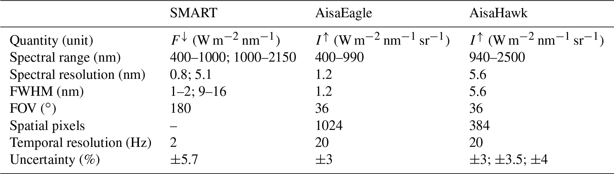
The Spectral Modular Airborne Radiation measurement sysTem (SMART) albedometer was installed to measure the solar spectral downward and upward irradiance with 2 Hz temporal resolution (Wendisch et al., 2001; Bierwirth et al., 2009; Ehrlich et al., 2019; Jäkel et al., 2021). For each hemisphere, an optical inlet was mounted on the aircraft fuselage, connected via optical fibers to two respective spectrometers (Wendisch and Mayer, 2003). A wavelength range from 400 to 2150 nm is covered with a full width at half maximum (FWHM) for each spectrometer of 1–2 and 9–16 nm, respectively. The optical inlets were actively stabilized to account for the varying aircraft attitude with an accuracy of ±0.2 % (Wendisch et al., 2001) for pitch and roll angles in a range of ±4.5^∘. Considered uncertainties account for the cosine correction (4 %) and sensor tilt (2.5 %). Further uncertainties include the wavelength accuracy as well as contributions from the radiometric calibration. The laboratory calibration was transferred to field conditions using a transfer calibration regularly performed during the airborne campaign (see Sect. 5.2). A total uncertainty of ±5.7 % for the downward irradiance in the near-infrared spectral range was estimated by Jäkel et al. (2021).

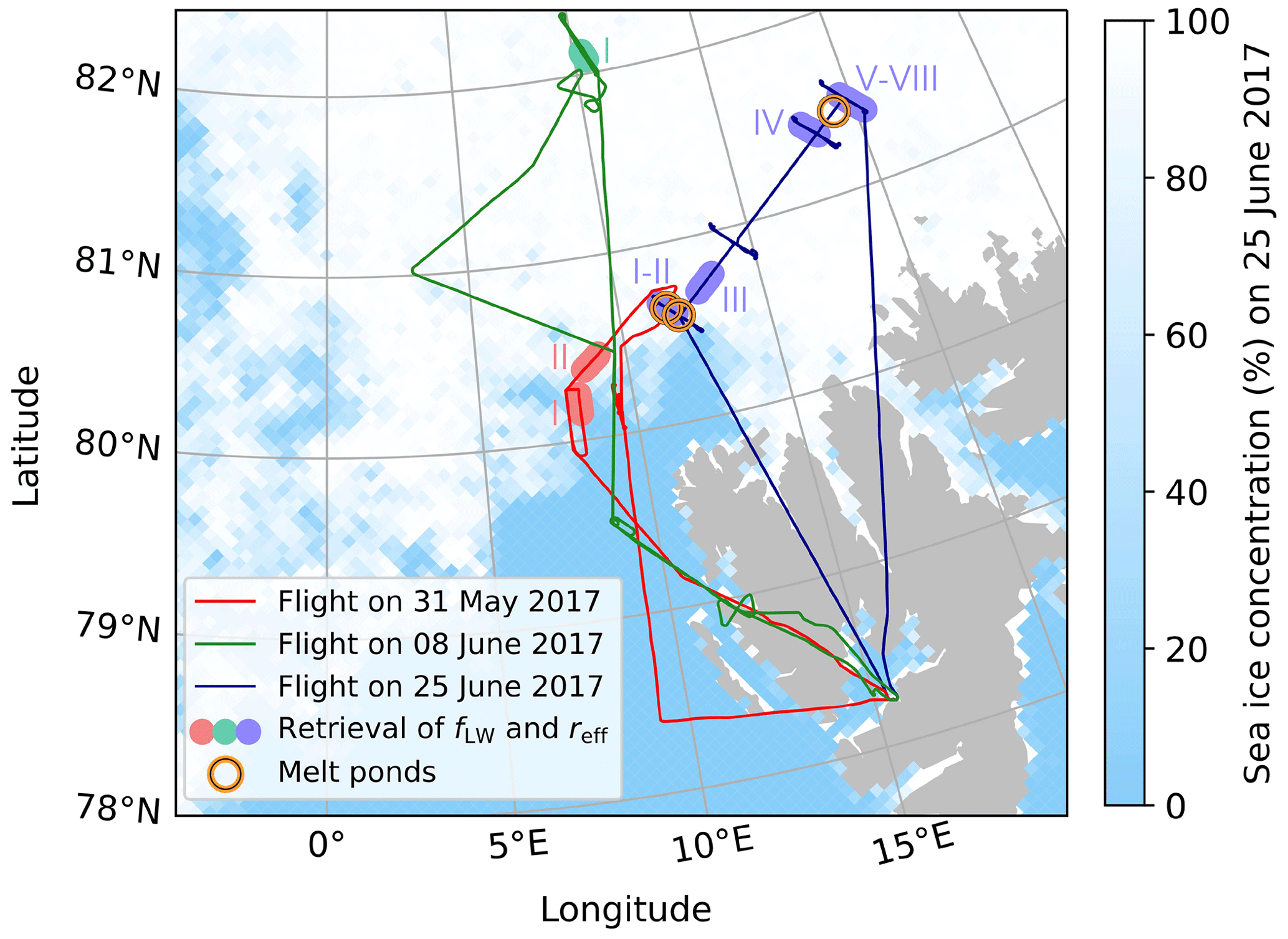
Figure 2 Map showing three flight tracks of the aircraft Polar 5 during the ACLOUD campaign with highlighted and numbered segments (several overflights in the case of the flight on 25 June 2017), for which the liquid water fraction f_LW and the effective radius r_eff were retrieved. Locations of the selected melt ponds are marked by open orange circles. In the background, the AMSR2 sea ice concentration on the 25 June 2017 is shown (Spreen et al., 2008).

AisaEagle and AisaHawk are across-track push-broom imaging spectrometers with a field of view (FOV) of 36^∘, which is spatially divided into 1024 (AisaEagle) and 384 (AisaHawk) pixels. These instruments measure the upward radiance with 20 Hz temporal resolution, covering collectively a wavelength range from 400 to 2500 nm (Schäfer et al., 2013; Ehrlich et al., 2019; Ruiz-Donoso et al., 2020). The radiance measurements have a spectral, temporal, and spatial dimension. An AisaEagle or AisaHawk scene is composed of a swath of pixels moving forward due to the aircraft motion. Therefore, the area covered by a single pixel is determined by the FOV and the number of spatial pixels as well as the flight altitude and aircraft speed (Schäfer et al., 2013). The calibration of the instruments was performed with a certified diffuse radiation source, whose relative uncertainty varies spectrally. For the spectral range of the AisaEagle radiance relevant for this study, the calibration uncertainty amounts to ±3 % (500–990 nm). The radiance measured by AisaHawk is required for a wider spectral range, for which the calibration uncertainty varies between ±3 % (940–990 nm), ±3.5 % (1000–1100 nm), and ±4 % (1150–1700 nm).

2.2 Radiative transfer simulations

In order to simulate snow reflectivity spectra, the library of radiative transfer routines and programs (libRadtran) was used (Mayer and Kylling, 2005; Emde et al., 2016). Applying libRadtran to model the radiative transfer in a dense medium such as a snow layer requires that the far-field assumption applies, which presumes that particles are at distance and, therefore, that the scattering waves can be assumed to be planar. Additionally, the multiple scattering assumption needs to be valid that defines particles by their single scattering properties and assumes no interaction between the particles takes place. Both assumptions might be violated when increasing the cloud density more than 100-fold to represent a snow layer. The issue was addressed by Pohl et al. (2020), who showed corresponding effects can be neglected.

The optical properties of the snow layer were calculated for a gamma size distribution n(L) (Emde et al., 2016) with the maximal dimension L, effective area A, and volume V. The size of ice particles or liquid water spheres in the snow layer is represented by the effective radius r_eff,

$$\begin{array}{}\text{(2)}& r_{\mathrm{eff}}={\displaystyle \frac{\mathrm{3}}{\mathrm{4}}}{\displaystyle \frac{{\int }_{L_{min}}^{L_{max}}V\left(L\right)\cdot n\left(L\right)\mathrm{d}L}{{\int }_{L_{min}}^{L_{max}}A\left(L\right)\cdot n\left(L\right)\mathrm{d}L}}.\end{array}$$

For our purpose the database of optical properties available in libRadtran was expanded to simulate effective particle radii r_eff larger than 25 µm. The single scattering properties (single scattering albedo, extinction coefficient) and Legendre moments representing the scattering phase function of ice crystals with sizes up to 800 µm were taken from an external database (Yang et al., 2000). The “smooth droxtal” shape was selected since it accounts for the expected rounding of ice crystals during the snow aging process. Applied by Pohl et al. (2020), this particle shape is assumed to be an adequate choice. For liquid water spheres, the Mie tool (Wiscombe, 1980), provided by libRadtran, was used to derive respective single scattering properties. The δ–M approach (Wiscombe, 1977) was applied in the simulations in order to reduce the number of Legendre moments necessary for an adequate representation of the scattering phase function. The bulk optical properties were scaled accordingly. More detailed information on the simulation setup is provided in the Appendix A.

3 Retrieval of snow layer properties

3.1 Methodology

To retrieve maps of snow layer particle size and liquid water fraction, an approach by Green et al. (2002) was adapted. Their approach is based on a least-squares fit between measured and simulated snow layer reflection spectra in the near-infrared spectral range, in which the local maxima of liquid water and ice absorption indices are shifted by several nanometers. Thus, this spectral range of a snow layer reflection spectrum is characterized by the liquid water fraction and the effective radius of snow grains. A direct derivation of f_LW from the spectral shift of the reflection minimum was not feasible due to its nonlinearity and sensitivity with respect to grain size and viewing zenith angle. Furthermore, regarding the airborne reflectivity measurements applied here, the spectral resolution of the imaging spectrometers is too low to resolve the nearly sigmoidal spectral shift function. Therefore, the retrieval method by Green et al. (2002) was adapted and applied to selected measurement cases observed during ACLOUD and libRadtran simulations.

The selection of ACLOUD flight sections used in this study was based on certain criteria. Overall, only cloud-free conditions were considered to reduce the required input information for radiative transfer simulations. Furthermore, flight sections with temporal stability of aircraft heading and height as well as pitch and roll angles near 0^∘ were selected. Hence, 11 flight sections from flights on 31 May, 8 June, and 25 June 2017 were chosen. They are depicted in Fig. 2; the specific times of the selected flight sections are provided in Table 2.

For the retrieval of r_eff and f_LW, the AisaHawk measurements (20 Hz resolution) were averaged to fit the SMART measurements (2 Hz resolution). This reduces the influence of small spatial structures and three-dimensional (3D) effects. Both spectral data sets were interpolated to a common wavelength grid with a spectral resolution of Δλ=1 nm. Using the upward radiance from the AisaHawk instrument and the downward irradiance data from the SMART albedometer, the spectral reflectivity was calculated according to Eq. (1). In accordance to the libRadtran simulations, the reflectivity spectra of the AisaHawk swath were averaged to 13 viewing zenith angles between $\mathit{\alpha }=-\mathrm{15}$^∘ and +15^∘ in Δα=2.5^∘ steps to reduce the influence of local inhomogeneities. This resulted in a nadir pixel area of 4.4 m × 30 m (across × along track) for a flight altitude of 100 m, aircraft speed of 60 m s⁻¹, and 0.5 s integration time.

Regarding the simulations, temporally constant conditions throughout each individual flight section were assumed, and, hence, the respective reflectivity spectra were calculated for the averaged solar azimuth and zenith angle and the aircraft height and heading. The observation geometry in the simulations was indicated via viewing azimuth angle (aircraft heading ±90^∘) and viewing zenith angle of the imaging spectrometers in order to consider the correct viewing geometry relative to the Sun position. Further information is provided in Table A1. The melting snow layer was assumed to be a mix of liquid water spheres between droxtal-shaped ice particles. Donahue et al. (2022) also applied the approach by Green et al. (2002) and showed this interstitial sphere model to be the most reliable out of three different models they tested in comparison to laboratory and field experiments.

This way, a lookup table (LUT) was simulated with libRadtran for varying viewing zenith angles, effective radii, and liquid water fractions. In the LUTs, the liquid water fractions were varied between f_LW=0 % to 30 % in Δf_LW=2.5 % steps, and effective radii ranged from r_eff=50 to 800 µm in Δr_eff=50 µm steps. Moreover, for each f_LW step, the 16 simulated spectra of varying r_eff were transferred to a resolution of Δr_eff=1 µm by cubic interpolation. The total water content was set to TWC = 100 000 g m⁻³ and the snow thickness to 1 m. The albedo of the underlying surface was chosen to be zero. This is justified because the TWC was chosen to be sufficiently high to ensure that the reflectivity is independent of the underlying surface albedo as most of the scattering takes place in the upper few centimeters of the snow layer.

In order to reduce the influence of the wavelength-dependent systematic errors in the instrumental calibration, measured and simulated reflectivity spectra were normalized by the measured or respectively simulated reflectivity value at the wavelength λ=1100 nm, where the absorption indices of liquid water and ice are almost identical. Hence, the information on effective radius and liquid water fraction is represented by the spectral shape of the normalized reflectivities rather than by their absolute values. Therefore, the normalization enables a more distinct separation of the sensitivity to both properties in the regarded wavelength ranges. Additionally, the simulated LUTs were convoluted according to the AisaHawk slit function (Ehrlich et al., 2019) in order to improve comparability between simulations and aircraft measurements.

For the coupled retrieval of r_eff and f_LW, three wavelength ranges were selected for the least-squares fit (Fig. 3): λ=982–1054 nm (Part 1), λ=1181–1240 nm (Part 2), and λ=1294–1320 nm (Part 3), omitting areas with strong atmospheric absorption. Part 1 covers the reflectivity minimum for pure ice at 1030 nm, making it sensitive to f_LW, while Parts 2 and 3 cover a spectral region that shows a strong dependence on r_eff with only minor sensitivity to f_LW.

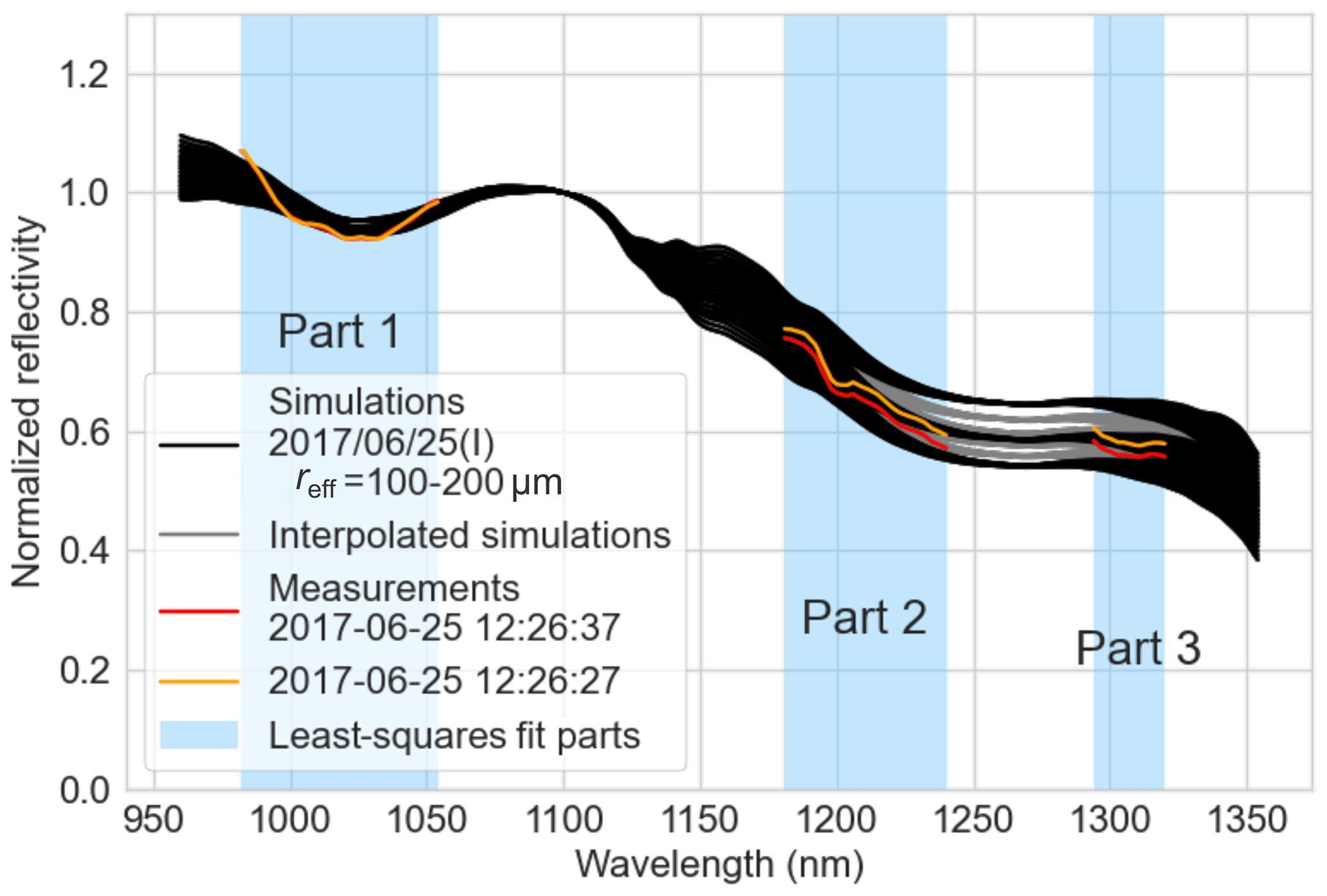
Figure 3 Comparison of measured (red and orange) and simulated (black) reflectivity spectra for flight section 2017/06/25 (I) for nadir measurements. Each black spectrum accounts for a certain combination of r_eff and f_LW in the simulations. Interpolated spectra were calculated for Δr_eff=1 µm, but only Δr_eff=10 µm steps are displayed in gray to enable visual distinction. The red and orange reflectivity spectra each correspond to one exemplary time step (given in UTC) of the flight section 2017/06/25 (I). The wavelength ranges used for the least-squares fit to retrieve r_eff and f_LW are indicated (Part 1–3 in blue).

3.2 Retrieval results

We applied the least-squares retrieval method to derive spatial maps of r_eff and f_LW for 11 selected flight sections. A statistical overview of the results is given in Table 2. Exemplarily, Fig. 4 shows the AisaEagle RGB (red, green, blue) composite, maps, and frequency distributions of r_eff and f_LW for flight section 2017/06/25 (I). The parameter maps show the derived properties for 13 viewing zenith angles between −15 and +15^∘ converted to the distance from nadir on the y axis and the along-track distance on the x axis. In the r_eff and f_LW maps, open water and melt ponds were filtered out and indicated as white areas in the r_eff map and as black areas of f_LW up to 100 % in the f_LW map.

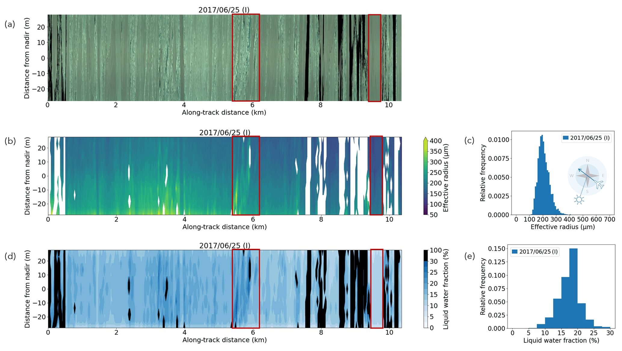
Figure 4 Flight section 2017/06/25 (I): (a) AisaEagle RGB composite (without spectral weighting for true color impression). Maps and frequency distributions of (b–c) r_eff and (d–e) f_LW. The maps are plotted over along-track distance and distance from nadir; the flight direction and Sun position are indicated in panel (c). Sections containing melt ponds or open water are excluded and shown in white in (b) and black in (d), corresponding to f_LW=100 %. For better contrast, the color bar of f_LW is compressed from 30 % on. Red highlighted areas include specific surface structures as melt ponds and pressure ridges (left) and rather homogeneous snow layer conditions (right).

The r_eff frequency distribution in Fig. 4c shows effective radius values between 100 and 400 µm, with occurrence of generally higher values towards the northeast (negative distances from nadir) as depicted in the map in Fig. 4b. This r_eff gradient is visible on all southeast- or northwest-heading flight sections, with the Sun located in the azimuthal range from south to west (see Table A1). It might therefore be an effect of geometry, rather than an actual overall gradient of the effective radius. The simulated reflectivity spectra show a dependence on viewing zenith angle with deviations about Δr_eff=100 µm between a viewing zenith angle of +15 and −15^∘. In addition, the nearer the scattering angle towards the forward-scattering peak, the stronger a non-complete representation of the phase function will influence the simulated reflectivity spectra. For future application, the influence of different particle shapes on the retrieved r_eff and f_LW should also be investigated.

The map and frequency distribution of retrieved snow layer liquid water fraction f_LW presented in Fig. 4d–e show values mostly between f_LW=5 %–30 %. In general, due to increased uncertainty of the AisaHawk calibration function for larger viewing zenith angles, the least-squares fit showed higher residuals towards the FOV edges, leading to higher uncertainties in these angle ranges.

Structures like melt ponds or pressure ridges, visible in the AisaEagle RGB composite, are also obvious in the r_eff and f_LW maps, as indicated by the left red box. At this point, possible 3D effects should also be considered, which could have been introduced by surface inhomogeneity and roughness and may be the reason for higher retrieved r_eff and f_LW values. In contrast, the right red box highlights a particularly homogeneous area, which is also represented in the maps of retrieved r_eff and f_LW.

Table 2 presents an overview of all analyzed cases including the mean, median, and standard deviation for all r_eff and f_LW maps. The retrieved effective radii were mostly between 50–700 µm and flight section averages of the order of 100–400 µm. This is a realistic magnitude compared to findings of particle sizes from Mei et al. (2021) and Jäkel et al. (2021) for an Arctic field campaign in March–April 2018. They derived the snow grain size from measurements of the Sea and Land Surface Temperature Radiometer (SLSTR) instrument on board Sentinel-3 and airborne SMART albedo measurements, respectively, and found snow grain sizes of 2017; thus 2 months later in the melting season, larger grain sizes can be thus 2 months later in the melting season, larger grain sizes can be expected due to snow metamorphism.

Table 2 Overview of statistics of the analyzed flight sections (SD – standard deviation).

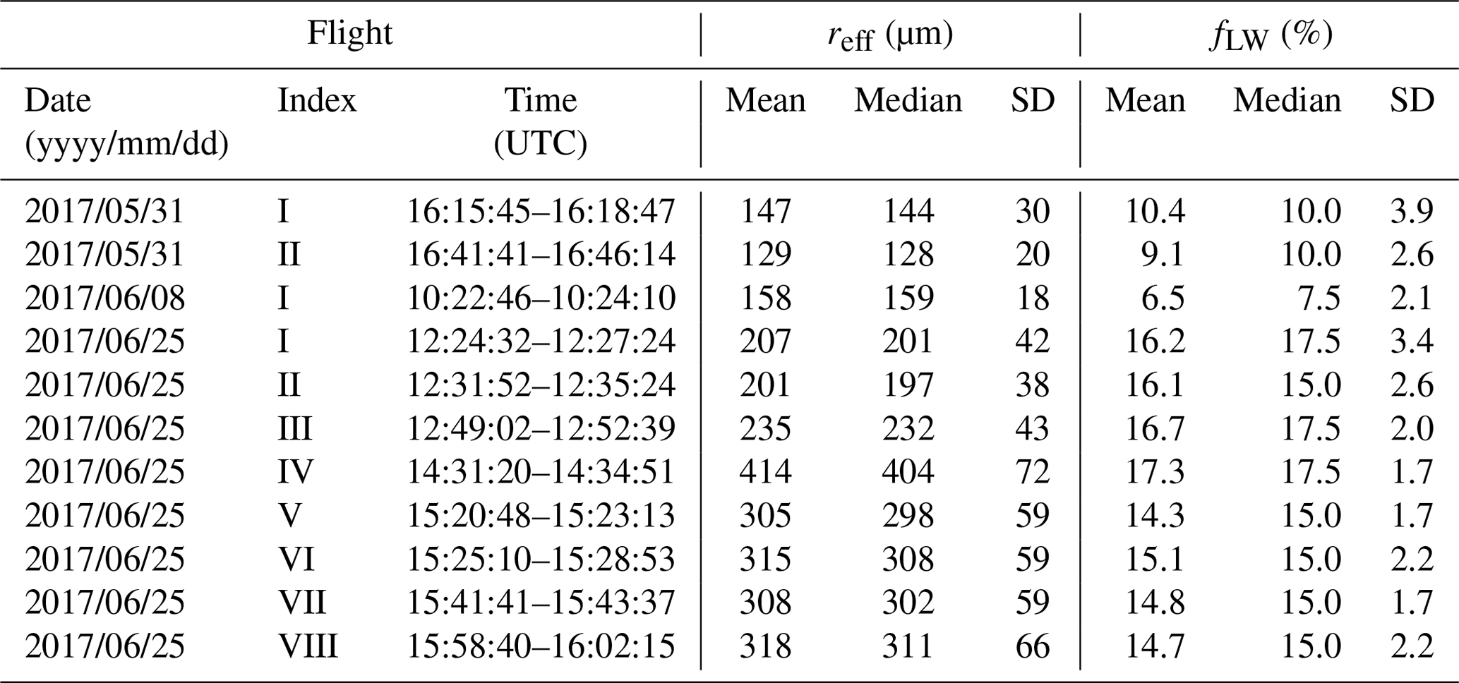
The retrieved liquid water fractions, averaged over the respective flight sections, were between 6.5 % and 17.3 %, corresponding to wet (3 %–8 %), very wet (8 %–15 %), and soaked (>15 %) snow layers according to the international classification for seasonal snow on the ground (Fierz et al., 2009). With the lowest mean liquid water fraction, during the flight section 2017/06/08 (I) a wet snow layer was probably observed. Regarding the flight sections (I) and (II) on 31 May 2017 the overflown snow could be characterized as very wet. A very wet to soaked snow layer can be assumed for the eight flight sections on 25 June 2017. This is in good agreement with the observation of numerous melt ponds during these flight sections (f_LW=14.3 %–17.3 %) in comparison to almost no melt ponds covered by the flight sections on 31 May and 8 June 2017 (f_LW=6.5 %–10.4 %). But especially for flight sections with no observable melt ponds, liquid water fractions above 8 % could have overestimated the actual snow wetness or be attributed to small or freshly refrozen leads that were not detected as areas of open water. However, since the approach is mostly sensitive to the uppermost snow layers, high retrieved f_LW values could be explained by the daily melting cycle rather than being due to an overall soaked snowpack. Generally, the retrieved liquid water fractions indicate progressed melting probably reaching the runoff phase except for flight section 2017/06/08 (I).

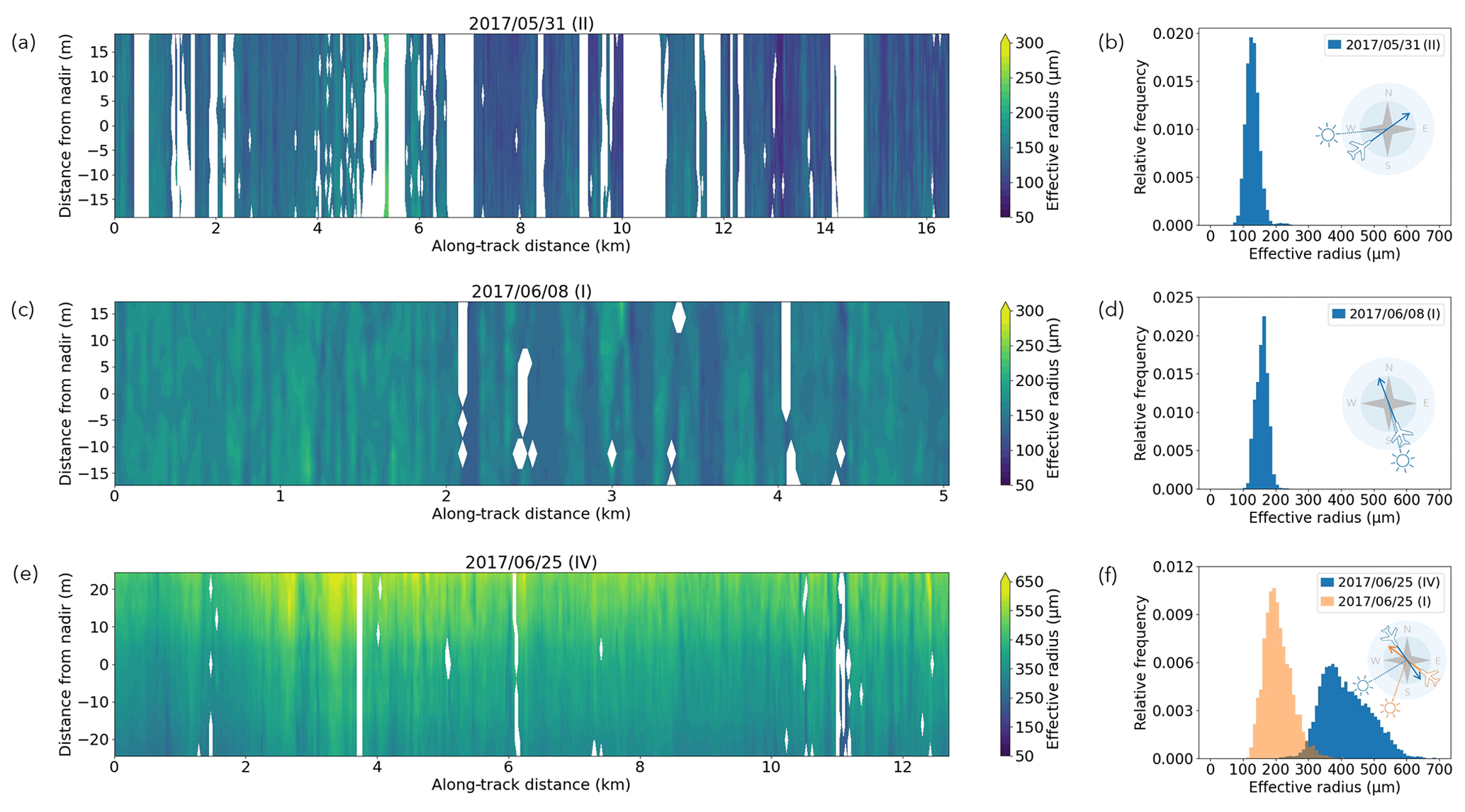
Figure 5 Maps of r_eff and respective frequency distributions for flight sections (a–b) 2017/05/31 (II), (c–d) 2017/06/08 (I), and (e–f) 2017/06/25 (IV). In the case of section 2017/06/25 (IV), the color bar maximum was adapted to account for overall higher r_eff. The r_eff frequency distribution of flight section 2017/06/25 (I) (map shown in Fig. 4) is also shown in (f) to represent geographical variability. In addition, the respective flight direction and Sun position are indicated for each flight section.

Since flight sections were selected from three different dates (31 May, 8 June, and 25 June 2017), a first attempt was made to investigate the temporal and regional variability of the derived parameters based on the presented case studies. Figure 5 shows r_eff maps of three flight sections (Fig. 5a, c, e) and frequency distributions of the data displayed in these maps (Fig. 5b, d, f). An overall increase in r_eff and broadening of the size distribution is visible from flight section 2017/05/31 (II) to 2017/06/25 (IV) and is interpreted to represent the expected snow metamorphism throughout the melting season. However, the derived r_eff seems to depend on the geographical location and local variations. In Fig. 5f the frequency distribution of flight section 2017/06/25 (IV) is plotted together with the distribution of flight section 2017/06/25 (I) (r_eff map shown in Fig. 4), which was conducted 2 h earlier and around 100 km southwesterly. The two particle size distributions show significant differences, with the 2017/06/25 (I) case consisting of overall smaller particle sizes and a narrower distribution in comparison to the 2017/06/25 (IV) distribution. Both flight sections have similar temporal length and across-track coverage. Therefore, differences can be attributed only to local characteristics. Hence, temporal variations are concealed by the seemingly stronger effects of geographical location.

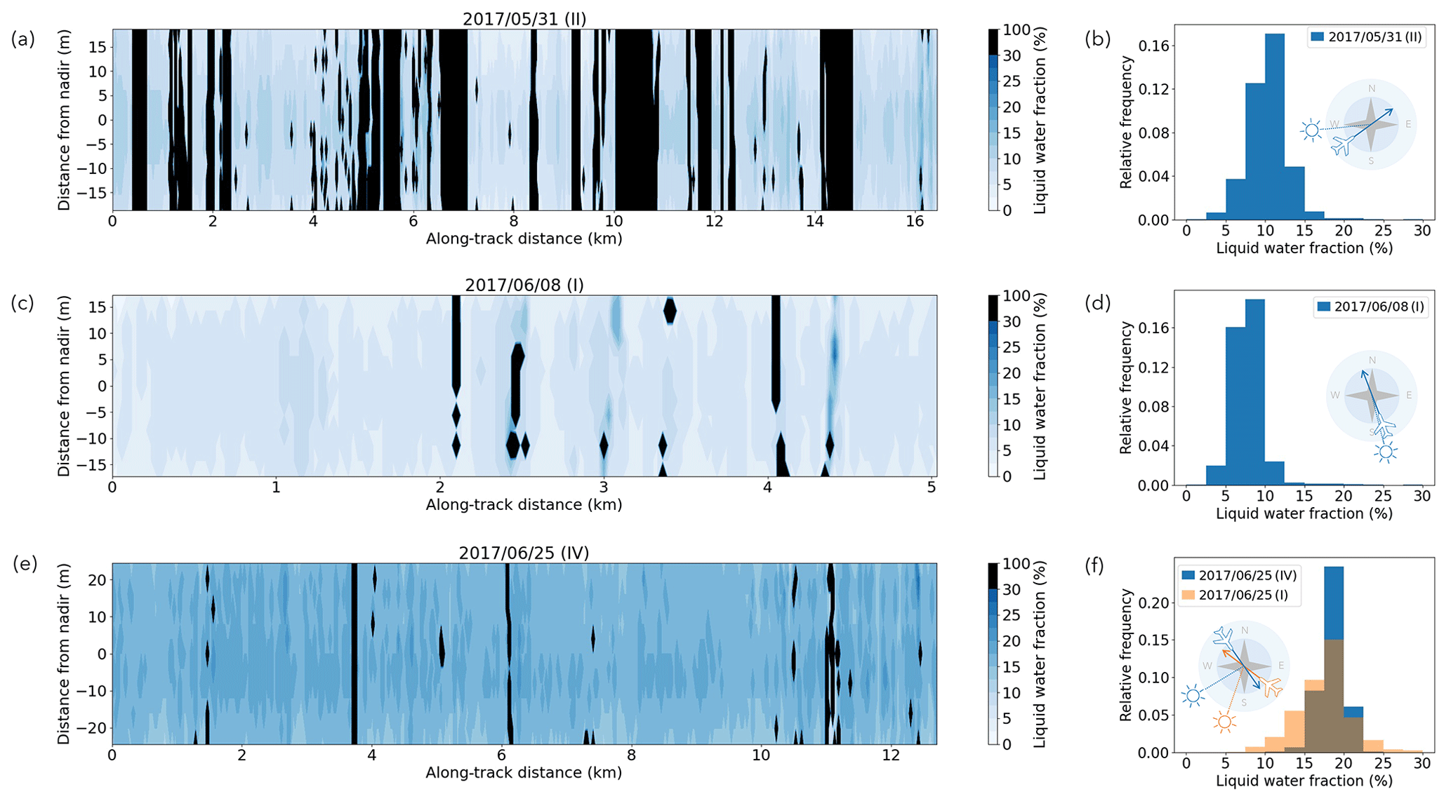
Figure 6 Maps of f_LW and respective frequency distributions for flight sections (a–b) 2017/05/31 (II), (c–d) 2017/06/08 (I), and (e–f) 2017/06/25 (IV). In the case of section 2017/06/25 (IV), the f_LW frequency distribution of flight section 2017/06/25 (I) (map shown in Fig. 4) is also shown in (f) to represent geographical variability. In addition, the respective flight direction and Sun position are indicated for each flight section.

Figure 6 shows f_LW maps and frequency distributions for the same flight sections that were presented in Fig. 5. Similar to r_eff, the distribution of f_LW also seems to be influenced rather by location than season. Here, the expected increase in mean f_LW during the season is not represented, and even a decrease during the flight section on 8 June 2017 is visible. However, also in this case, the influence of geographical location might again overlay any visible effect of temporal changes throughout the melting season, since the flight section on 8 June 2017 was carried out further north than the other two (see flight map in Fig. 2), where lower f_LW could be expected. Figure 6f shows the f_LW distributions of flight sections 2017/06/25 (IV) and 2017/06/25 (I) (f_LW map in Fig. 4). Some geographical variability is apparent, with the f_LW distribution of section 2017/06/25 (IV) being narrower than that of section 2017/06/25 (I). This could also be connected to the higher melt pond fraction of 0.76 % for flight section 2017/06/25 (I) compared to 0.41 % for 2017/06/25 (IV), which could indicate a differing melting progress. However, the effect seems less pronounced compared to the r_eff distribution in Fig. 5f. A daily cycle due to undamped solar radiation in cloud-free conditions could also overlay seasonal effects.

4 Retrieval of melt pond depth

4.1 Methodology

The spectral melt pond reflectivity is mainly determined by the pond ice bottom reflectivity and only limited by the pond depth (Lu et al., 2016, 2018). To retrieve the melt pond depth, König and Oppelt (2020) analyzed the spectral slopes of log-scaled simulated reflectivity spectra of ponds with different pond ice bottom characteristics and depths at the wavelength λ=710 nm, where pond water absorption causes distinct attenuation implying a depth dependence. They found a property that is nearly independent of the pond ice bottom characteristics and strongly correlated with the pond depth z. This relation can be described by a linear equation:

$$\begin{array}{}\text{(3)}& {\displaystyle }z=a\left({\mathit{\theta }}_{\mathrm{Sun}}\right)+b\left({\mathit{\theta }}_{\mathrm{Sun}}\right){\left[{\displaystyle \frac{\partial \log \left({\mathcal{R}}_{\mathit{\lambda },*}\right)}{\partial \mathit{\lambda }}}\right]}_{\mathit{\lambda }=\mathrm{710}\mathrm{nm}},\end{array}$$

with ${\mathcal{R}}_{\mathit{\lambda },*}={\mathcal{R}}_{\mathit{\lambda }}\cdot (\mathit{\pi }\mathrm{sr}{)}^{-\mathrm{1}}$. The fitting parameters a and b depend on the solar zenith angle θ_Sun, and the melt pond depth z is retrieved in units of centimeters (König and Oppelt, 2020). Evaluating the accuracy of this linear model, König and Oppelt (2020) compared retrieved depths to in situ measurements and stated a coefficient of determination of 0.65. Zhang et al. (2022) also applied a modified version of the linear model to albedo measurements. In comparison to other approaches, they found limited reliability and pointed out model-based limitations. However, Linhardt et al. (2021) found a reasonable agreement of melt pond depths retrieved by the linear model with measurements of a ground-based echo sounder within a range up to 1 m depth. These measurements were performed during the Multidisciplinary drifting Observatory for the Study of Arctic Climate (MOSAiC) campaign in 2019/20 (Nicolaus et al., 2022). Furthermore, König et al. (2020) applied the linear model to airborne imaging spectrometer observations focusing on the comparison of different atmospheric correction techniques as measurements of the downward irradiance were affected by the operated helicopter. Regarding this study, with the AisaEagle upward radiance and the SMART downward irradiance, both components of the reflectivity (see Eq. 1) were measured and used as input for the linear model to retrieve the depth of selected melt ponds captured during the ACLOUD campaign.

An application of the linear model by König and Oppelt (2020) is constrained by certain assumptions and limitations, which led to specific criteria for the selection of overflown melt ponds during the ACLOUD campaign. First, the model is only applicable under cloud-free conditions as clouds would cause deviating in-water pathways due to diffuse incidence. Also specular reflections at the water surface would be more likely in purely diffuse illumination conditions. That aspect is of importance because measurements of the upward radiance performed above the melt pond also capture water surface reflections. As only the water leaving radiance is of interest to retrieve pond properties, this component has to be minimized in order to increase the sensitivity to the pond depth. However, observing a stagnant water body within a narrow FOV under cloud-free conditions can be regarded as optimal conditions for avoiding glint perturbations (Zibordi et al., 2019; Pitarch et al., 2020). Therefore, specular reflections could be neglected here, as suggested by König and Oppelt (2020). Furthermore, in the narrow angular range captured by AisaEagle the reflective behavior of ponded ice is almost isotropic (Goyens et al., 2018). Consequently, all measurements were assumed to represent nadir conditions, although the viewing zenith angle varied. Second, pure melt pond water without any dissolved matter is assumed. This way, the depth retrieval is based on water absorption along the traversed pathway through the pond. Due to increasing absorption with depth, König and Oppelt (2020) stated a model applicability for depths reaching a maximum of 1 m. Therefore, only ponds with apparently light blue color were selected to limit the probability of mixing with ocean water. Third, based on the general horizontal plane assumption, flight sections with aircraft pitch and roll angles exceeding 4.5^∘ in absolute values were excluded from the retrieval. Figure 2 shows the selected melt pond locations along the flight track on 25 June 2017. In total, five ponds were selected, of which three were overflown consecutively and are depicted by a single orange circle.

To perform the melt pond depth retrieval, the downward irradiance of SMART was interpolated to match the temporal resolution of AisaEagle (see Table 1). This ensured a sufficiently high spatial resolution to resolve single melt pond pixels. Thus, the pixel size of the AisaEagle measurements determined the minimum resolvable pond size. For a flight altitude of 100 m, aircraft speed of 60 m s⁻¹, and 0.05 s integration time, a nadir AisaEagle pixel would cover an area of 0.06 m × 3 m (across × along track). Melt ponds were identified with a mask algorithm, which classified the surface into open ocean water, sea ice/snow, and melt ponds according to surface typical reflectivity spectra. Pond pixel clusters were found with their respective reflectivity spectra, which were calculated according to Eq. (1) and spectrally interpolated to Δλ=1 nm.

Furthermore, based on a comparison with libRadtran simulations, possible atmospheric effects, occurring between surface and flight level, could be neglected. Representing near-surface conditions, the determined reflectivity spectra were processed as suggested by König and Oppelt (2020). First, a moving mean filter with a window size of 5 nm was used to smooth the reflectivity spectra. Second, to obtain the spectral slope at λ=710 nm, a Savitzky–Golay filter was applied, fitting a second-order polynomial to the log-scaled reflectivity spectrum and determining the first derivative of a 9 nm window. The slope as well as the solar zenith angle, which ranged between 57.7 and 63.2^∘, were inserted into the linear model by König and Oppelt (2020) (Eq. 3) to retrieve the depth of the five selected melt ponds and their depth statistics. The retrieved depth z is defined here as the depth of a single pond pixel, i.e., pixel depth, of which the spectral reflectivity was measured.

4.2 Retrieval results

In a case study, the depth of the melt pond P1 was retrieved, which was also covered during flight section 2017/06/25 (I) shown in Fig. 4 inside the left red box. The pond has a surface area of 225.4 m² and is surrounded by pressure ridges, as shown in Fig. 7a. For each pond pixel, the water depth was retrieved with the linear model by König and Oppelt (2020) yielding the pond depth shown in Fig. 7b. The maximum depth of 0.33 m was derived for the pond center. Pond parts to the right at between 30 and 45 m along-track distance are mostly shallower, with depths varying around 0.2 m. Overall, the melt pond depth is characterized by a high spatial variability and also inversely represents the underlying sea ice relief.

Figure 7c connects depth statistics of the five selected melt ponds P1 to P5 to their contained total meltwater volume. Pond P1, already analyzed, contains the largest meltwater volume of 47.8 m³ because of its spatial expansion and rather deep parts. The box-and-whisker plot with median and mean depth points out a rather symmetrically distributed depth. The main fraction of the pixel depths is located within the whisker range. However, a few outliers of shallower pixels occur. Pond P3 stores the second largest volume with 6.0 m³ despite covering a smaller area of 39.1 m² than P5 with an area of 50.6 m² and a meltwater volume of 4.9 m³. But a distinct fraction of P3 pond pixels is located at larger depths, resulting also in a skewed distribution as indicated by median and mean positions. Conversely, the pixel depths of pond P5 rather show a bimodal distribution. Melt pond P4, storing 2.4 m³, is smaller in surface area with 22.2 m², and the depth distribution is nearly symmetrical. In contrast to P1, the smallest pond in terms of area (13.6 m²), volume (1.2 m³), and, therefore, also depth range is P2. This comparison points out the high variability of the geometrical melt pond dimensions depending on local factors, especially on ice surface roughness and the available amount of meltwater.

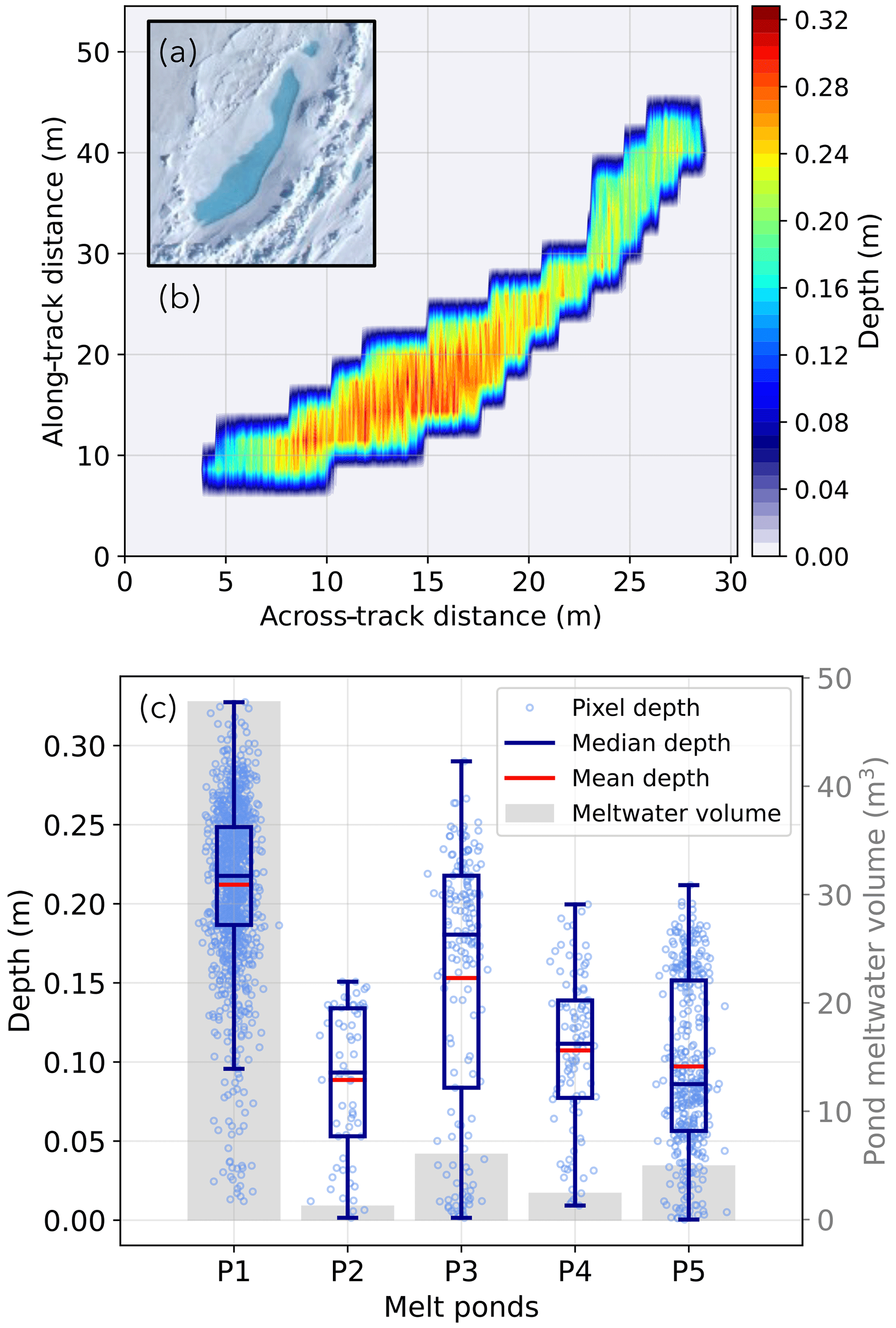
Figure 7 (a) Image captured by a digital camera with a fisheye lens mounted on Polar 5. (b) Mapped depth distribution of melt pond P1 according to the pixel sizes in the along- and across-track direction, with a color bar displaying the depth. (c) Pixel-based depths (light-blue dots) of the five selected melt ponds P1 to P5 plotted together with box (first to third quartile) and whisker (1.5 times the interquartile range) plots visualizing the depth distribution with indicated mean (red) and median (dark blue) depth. The gray bars represent the total meltwater volume contained in the respective pond.

As no ground-based reference measurements were performed during the ACLOUD campaign, only in situ pond depth measurements of other campaigns can provide a guideline to evaluate the here retrieved pond depth. The studies by König and Oppelt (2020) and König et al. (2020) obtained reference in situ measurements with a folding ruler on 10 June 2017 with a maximum pond depth of about 0.35 m. During the MOSAiC campaign in 2019–2020, the sea ice surface observations also comprised melt pond depth measurements in late June and yielded mean depths of about 0.1 to 0.15 m (Webster et al., 2022). Therefore, the magnitude of the depths retrieved here can be assumed to be quite reasonable at the start of the pond evolution.

5 Discussion of technical limitations

An estimation of the reliability of the retrieval methods described here is restricted due to the lack of ground-based reference measurements during the ACLOUD campaign. Instead, the derived r_eff and f_LW maps as well as the melt pond depth were compared to typical values from the literature. Additionally, the potential sources of uncertainties and retrieval biases are quantified and discussed in the following.

5.1 Snow layer properties

Considering the different sources of uncertainty imposed by the retrieval approach that add to the uncertainty of the airborne measurements, a deviation from the actual r_eff and f_LW can be expected. In the following, the sources of uncertainty are estimated with sensitivity studies. An overview of uncertainty sources and their contribution is provided in Table 3.

Table 3 Overview of different sources of uncertainty and their influence on the derived effective radii and liquid water fractions given as maximum uncertainty and RMSE (root mean square error).

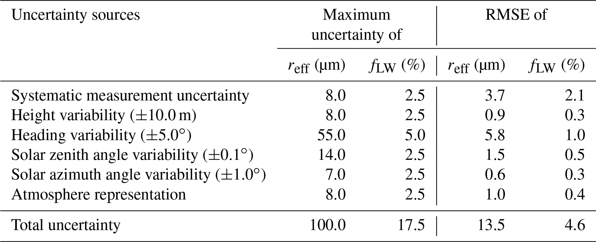
First, the impact of the SMART and AisaHawk measurement uncertainties on the derived parameters was quantified by spectrally adding and subtracting the maximum possible bias (between 5.7 % + 3 % = 8.7 % up to 5.7 % + 4 % = 9.7 %; see Table 1) from the reflectivity spectra and then again performing the retrieval approach. This led to deviations of Δr_eff=8 µm and Δf_LW=2.5 %, which demonstrate the effectiveness of normalizing the reflectivity spectra in order to reduce the influence of systematic errors. Statistical errors were rather small (about 0.1 %), and creating modified reflectivity spectra with a Gaussian error distribution (SD = 0.1 %) did not change the derived r_eff and f_LW significantly.

In a similar way, the influence of averaging the aircraft height and heading and the solar zenith and azimuth angle for the simulations was examined by varying those properties in the simulations between the maximal and minimal value during the flight sections. The retrieval method was performed again for these adapted LUTs, leading to the maximal uncertainties and RMSE (root mean square error) values in the derived properties that are listed in Table 3. The strongest sources of uncertainty are deviations from the aircraft heading due to the sensitivity of the retrieval method to the phase function of the scattering particles.

Furthermore, the representation of atmospheric conditions in the simulations was analyzed. The simulations, used in the retrieval, were performed assuming a standard Arctic summer atmosphere in combination with radiosonde profiles from Ny-Ålesund for the respective flight day. To evaluate the importance of information on local conditions, additional simulations were performed with the standard atmosphere only. A comparison of both atmosphere representations in the simulations yielded the given deviations for retrieved r_eff and f_LW.

The total uncertainty given at the bottom of Table 3 shows a high susceptibility of the retrieval method to the examined uncertainty sources and rather strong deviations for single pixels on the map (maximum uncertainty), possibly due to 3D effects. The RMSE is generally lower than the maximum uncertainty in the order of 10 % for r_eff and 30 % for f_LW. However, the uncertainty of the liquid water fraction might be overestimated because the retrieved values are restricted to the resolution of Δf_LW=2.5 % of the simulations. Increasing the f_LW resolution would probably reduce the total error margin. Moreover, reducing the measurement uncertainty and increasing the wavelength resolution of the measurement devices could further improve the reliability of the retrieval method. In addition to that, only choosing flight sections with very stable headings, only minor changes in solar azimuth and zenith angles and shorter examined flight sections would further increase the steadiness of the retrieved parameters.

5.2 Melt pond depth

Uncertainties affecting the retrieved pond depth can be ascribed to systematic measurement uncertainties of AisaEagle and SMART in the range of ±3 % and ±5.7 %, respectively. A total uncertainty of ±8.7 % was applied to the whole reflectivity spectrum. However, the effect on the pond depth was negligible as the linear model by König and Oppelt (2020) is based on the spectral slope of the log-scaled reflectivity. An uncertainty of ±2 % arising from the SMART transfer calibration (Sect. 2.1), which is connected to the temperature dependence of the spectrometer, was applied to vary the steepness of the reflectivity spectrum in the spectral range of 9 nm around λ=710 nm that was scanned by the Savitzky–Golay filter. For this uncertainty component, a maximum depth deviation of the selected ponds of about ±0.07 m was found and showed a dependence on the respective solar zenith angle, which was the second input property of the linear model. With increasing solar zenith angle, the deviation of the pond depth due to a differing reflectivity slope decreased.

Furthermore, the calculation of the reflectivity spectrum slope by the Savitzky–Golay filter itself should also be regarded as a potential uncertainty affecting the retrieval. The filter was applied, as suggested by König and Oppelt (2020), with a polynomial order of 2 and a scanned window size of 9 nm. Thus, at the selected wavelength, a polynomial fit was applied to a 9 nm interval of the log-scaled reflectivity spectrum, and the first derivative, i.e., the slope, was determined. The selection of the window size was based on the compromise between noise removal and the preservation of important spectral features. In that context, a 9 nm window was an adequate choice. However, to quantify the effect of the window size, the melt pond depth was also retrieved with a 3 nm window, i.e., applying no smoothing. The retrieved depth deviated at a maximum of about 0.11 m. Therefore, the smoothing is affecting the retrieval distinctly and has to be applied specifically depending on instrument and measurement conditions.

6 Conclusion

In this study, snow layer and melt pond properties were retrieved based on airborne imaging spectrometer observations. The retrieval approach for liquid water fraction and effective radius of snow grains is based on a method introduced by Green et al. (2002), exploiting the spectrally differing absorption indices of ice and liquid water in the near-infrared spectral range. Snow layer reflectivity LUTs were simulated for varying liquid water fractions and effective radii to identify the spectral ranges with the strongest sensitivity to both parameters. Measured snow reflectivity spectra were compared to simulations via a least-squares fit, and the respective liquid water fraction and effective radius values were derived as the minimum residual. The determined parameters were mapped for 11 flight sections on 3 d of the ACLOUD campaign. The flight section averages of retrieved liquid water fractions ranged from 6.5 % to 17.3 % and the effective radii from 129 to 414 µm. These results were analyzed in the context of temporal snow layer development, but the effect was mainly masked by the geographical location of the measurements. The small number of cloud-free flight sections during the ACLOUD campaign did not allow us to average over different flight sections for each day with varying geographical locations and times. However, based on the performed case studies, the total uncertainty margin of the approach was evaluated by performing sensitivity studies that took uncertainty in measurements and simulations into account. In order to reduce the number of free variables, only droxtal-shaped ice particles were considered in the simulations here. Future studies should investigate the effect of different ice particle shapes on the retrieval method. Furthermore, the same effective sizes of ice and liquid water particles were assumed in this study. Donahue et al. (2022) used a similar model of same-sized ice and liquid water particles, which compared well to laboratory and field measurements. However, the actual relation between ice and liquid water particle size is unknown and might also vary with melting regime (Colbeck, 1978, 1979; Hannula and Pulliainen, 2019). It was concluded that a realistic representation of the reflective behavior of a melting snow layer in radiative transfer simulations is crucial for reliable retrieval results.

In the second part of this study, the melt pond depth was retrieved with the linear model developed by König and Oppelt (2020). This approach is almost independent of the pond ice bottom reflectivity and is based on the slope of the log-scaled reflectivity spectrum at 710 nm as well as the solar zenith angle. The pond depth and the in-pond depth distribution were analyzed for five selected cases, with a maximum retrieved depth of 0.33 m. It can be stated that the pond depth is a spatially highly variable property. The importance of a precise pond depth retrieval was highlighted, estimating the meltwater volumes stored in the observed melt ponds. Uncertainties affecting the retrieval included the measurement uncertainty and retrieval assumptions, comprising pure pond water and negligible water surface reflections. Another aspect concerns the data processing and especially the smoothing procedure, which can introduce further uncertainties. Also a complete independence of the pond ice bottom reflectivity cannot be guaranteed for the linear model, as stated by König and Oppelt (2020).

The two retrieval methods illustrate the potential of studying melting processes on sea ice by combining the retrieved snow grain size, liquid water fraction, and melt pond depth to obtain an overall picture. However, a validation with ground-based reference measurements would be required for further improvements of the approaches and their adjustment to airborne measurements. In future studies, different areas of sea ice should be overflown multiple times throughout the entire melting season to characterize the temporal development of snow layer composition and melt ponds. This would exploit the full potential of airborne imaging spectrometers, e.g., AisaEagle and AisaHawk, to map the Arctic sea ice surface transition, following the meltwater path from the snow layer to melt ponds.

Appendix A: Radiative transfer simulations

The spectral downward irradiance and upward radiance were simulated with the library of radiative transfer routines and programs libRadtran (Mayer and Kylling, 2005; Emde et al., 2016). To solve the radiative transfer equation, the discrete ordinate algorithm DISORT (Stamnes et al., 2000) was selected. For the intensity correction, Legendre moments were used (Nakajima and Tanaka, 1988). Furthermore, the extraterrestrial solar spectrum by Gueymard (2004) and the absorption parameterization by Gasteiger et al. (2014) were applied. Atmospheric conditions were described by standard profiles of pressure, temperature, relative humidity, air, and trace gas densities for the subarctic summer (Anderson et al., 1986). Additional atmospheric information was provided by radio soundings performed at Ny-Ålesund (Maturilli, 2020).

Table A1 Aircraft orientation and illumination conditions during the selected flight sections given with their respective standard deviation.

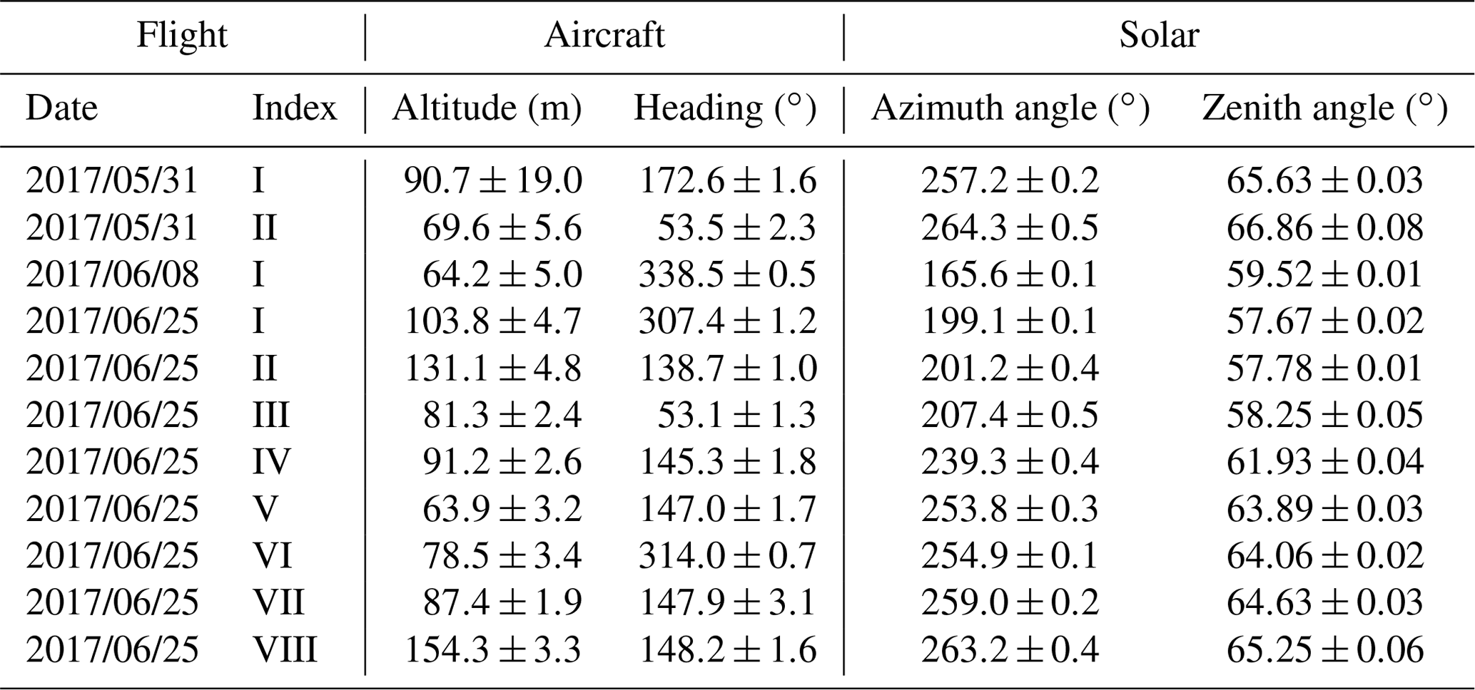
Further input parameters are listed in Table A1 and comprise the flight day and altitude as well as solar and viewing azimuth and zenith angles describing the Sun position and observation geometry with respect to the aircraft heading in order to simulate reflectivities comparable to the push-broom imaging spectrometer measurements.

To represent the snow layer, a mixed-phase cloud layer located at 0–1 m above the surface was defined by a constant total water content (TWC) of 100 000 g m⁻³ while varying the liquid water and ice water content to account for melting processes. An external mixture of liquid water and ice particles was assumed (Donahue et al., 2022). The extinction coefficient, the single scattering albedo, and the scattering phase function for a gamma size distribution of liquid water spheres and smooth ice droxtals were calculated with the Mie tool (Wiscombe, 1980), provided by libRadtran, and the Yang tables (Yang et al., 2000), respectively. These properties were derived with 2048 Legendre moments and δ–M scaling (Wiscombe, 1977) to ensure an adequate resolution of the phase function.