A retrieval of xCO₂ from ground-based mid-infrared NDACC solar absorption spectra and comparison to TCCON

Two global networks of ground-based Fourier transform spectrometers are measuring abundances of atmospheric trace gases that absorb in the near infrared and mid-infrared: the Network for the Detection of Atmospheric Composition Change (NDACC) and the Total Carbon Column Observing Network (TCCON). The first lacks a CO₂ product; therefore, this study focuses on developing an xCO₂ retrieval method for NDACC from a spectral window in the 4800 cm⁻¹ region. This retrieval will allow extending ground-based measurements back in time, which we will demonstrate with historical data available from Ny-Ålesund, Svalbard. At this site, both TCCON and NDACC measurements are routinely performed, which is an advantage for collocated comparisons. The results are compared with collocated TCCON measurements of column-averaged dry-air mole fractions of CO₂ (denoted by xCO₂) in Ny-Ålesund, Svalbard, and only TCCON in Burgos, Philippines. We found that it is possible to retrieve xCO₂ from NDACC spectra with a precision of 0.2 %. The comparison between the new retrieval and TCCON showed that the sensitivity of the new retrieval is high in the troposphere and lower in the upper stratosphere, similar to TCCON, as seen in the averaging kernels, and that the seasonality is well captured as seen in the retrieved time series. Additionally, we have included a retrieval strategy suggestion to improve the quality of the xCO₂ product.

1 Introduction

Carbon dioxide (CO₂) is the most important anthropogenic greenhouse gas. Fossil fuel combustion and deforestation are the main net sources of CO₂; the ocean and terrestrial ecosystems currently act as net sinks, absorbing approximately half of anthropogenic emissions (IPCC, 2022). Remote sensing measurements provide a column integral that is less affected by vertical transport and local sources. The CO₂ column derived from ground-based Fourier transform infrared (FTIR) spectrometry from near-infrared radiation (NIR) solar absorption spectra can achieve precision better than 0.25 % (Wunch et al., 2011a).

The Total Carbon Column Observing Network (TCCON), a worldwide network, currently has 26 measurement sites that have been operational since 2004. The network was founded for satellite validation and remotely measures abundances of CO₂, CO, CH₄, and other molecules absorbing in the near infrared, covering the spectral range from 4000 to 11 000 cm⁻¹.

The Network for the Detection of Atmospheric Composition Change Infrared Working Group (NDACC-IRWG) was founded in 1991 and has a total of 25 sites. The network provides total column abundances and profiles of several atmospheric constituents, with a focus on the O₃ cycle (De Maziere et al., 2018) retrieved from the mid-infrared, covering the spectral region 2000 to 5000 cm⁻¹. It uses an optical filter to limit the spectral range of the recorded spectrum. The NDACC official filters are listed in the Appendix of Blumenstock et al. (2021).

NDACC trace gas products, in contrast to TCCON, do not include CO₂. An extension of the retrieval capabilities of NDACC spectra to include an CO₂ product would expand the temporal and spatial coverage of the total column products. In this study one set of historical data for Ny-Ålesund is presented, where the CO₂ spectra date back to 1997. Two major challenges have to be faced on the way to an NDACC xCO₂ product. The TCCON retrieval method uses the ratio of CO₂ from the 6300 cm⁻¹ band and O₂ from the 7885 cm⁻¹ band (Yang et al., 2002); in contrast, there are no O₂ absorption lines present in the NDACC mid-infrared (MIR) spectra. Therefore, there is no proxy for the dry-air column with which to make a ratio. N₂ lines are present in the 4800 cm⁻¹ region; however, the lines are too weak. Additionally, the presence of multiple interfering gases hinders the use of broad spectral windows (Buschmann et al., 2016).

Previous efforts towards an xCO₂ product using MIR spectra include Barthlott et al. (2015) and Buschmann et al. (2016). The column-averaged dry-air mole fractions of CO₂ (xCO₂) retrieval proposed by Barthlott et al. (2015) using four microwindows in the 2620 cm⁻¹ region were appropriate for long-term monitoring of instrument stability and consistency of trends of tropospheric species. However, due to the low sensitivity of the MIR averaging kernels to the surface, the proposal by Barthlott et al. (2015) was not applicable for shorter timescales; therefore, it did not provide new information on the carbon cycle, as the annual trends are already well understood. Similarly, Buschmann et al. (2016) presented an approach for the retrieval of xCO₂ from several NDACC MIR microwindows in the 2620 to 3350 cm⁻¹ region. This approach was shown to have a strong sensitivity to the chosen a priori and low sensitivity in the troposphere due to the small averaging kernels in comparison to TCCON.

In this study a retrieval of the column-averaged dry-air mole fraction of CO₂ from MIR solar spectra in the 4800 cm⁻¹ region is described. We will discuss the different retrievals, their sensitivities, and dependence on the a priori information and air mass factor. We will present the averaging kernels, and their influence on the retrieval as well as our approach to an error budget, covering standard errors, the diurnal variation, sensitivity to several error sources, and finally their application to Ny-Ålesund historical data.

In the next section information on the selected sites is given, and the window and the retrieval used are described. Then in Sects. 3 and 4 the influence of the averaging kernels, the a priori, and air mass factor on the retrieval is investigated and compared to TCCON, respectively. Section 5 includes the error budget and error source tests. In Sect. 6 the time series for both Burgos and Ny-Ålesund historical data are presented, and an acquisition strategy is proposed in Sect. 7, followed by conclusions in Sect. 8.

2 Measurements and methods

2.1 Location and measurements

Data from two sites were used, Ny-Ålesund in the Arctic and Burgos in the tropics. Ny-Ålesund provides the collocated measurements of NDACC and TCCON. On the other hand, Burgos gives us the opportunity to assess the retrieval in an atmosphere with higher temperature and water content.

The measurements in Ny-Ålesund (Spitzbergen; 78.92^∘ N, 11.92^∘ E) were performed using the Bruker IFS 120-5 HR instrument with indium–gallium–arsenide (InGaAs) and liquid-nitrogen-cooled indium–antimonide (InSb) detectors. NDACC spectra have been recorded with the InSb detector since 1992, which covers the mid-infrared spectral region with an optical path difference (OPD) of 180 cm, giving a spectral resolution of approximately 0.005 cm⁻¹. The acquisition is performed with different band-pass filters. The filter of interest for this study transmits from 4044 to 4822 cm⁻¹; it will be referred to as filter 4433 according to its center wavenumber, and it started being used in 1996. On the other hand, TCCON has used the InGaAs detector for its measurements since 2004, covering the spectral region 4000 to 11 000 cm⁻¹ (Wunch et al., 2011a).

Burgos (Philippines; 18.53^∘ N, 120.65^∘ W) has a warm and humid climate. There, only TCCON InGaAs measurements are performed with a Fourier transform spectrometer (FTS) model Bruker 125 HR. The operations started in 2017 (Morino et al., 2018; Velazco et al., 2017). The tropics face different challenges with a higher water vapor content along the light path and a higher tropopause.

The spectra available were separated in two groups, InSb (from NDACC) and InGaAs (from TCCON); both were used to retrieve xCO₂ from the new window and compared to the xCO₂ retrieved from the two TCCON CO₂ windows from InGaAs spectra.

Additionally, collocated TCCON and aircraft profiles from campaigns over TCCON stations and AirCore were used where available to do a comparison with in situ data. This allows for the determination of the systematic biases in the spectroscopy of the column measurement as is similarly done for TCCON windows in the recent GGG2020 soon to be released.

2.2 CO₂ window in the MIR

The mid-infrared region not only has CO₂ absorption lines but also other gases with strong absorption lines. The high-resolution measurements of NDACC allow for the use of narrower windows or single lines. The selected spectral window is centered at 4790 cm⁻¹ and has a 20 cm⁻¹ width; hence, we will refer to it as w4790. It contains water lines but minimal interference from other gases.

To choose the windows, we made use of information on the NDACC filters and the intensity of the transitions of CO₂ in the region. The first step to select prospect windows was to study the NDACC spectra available from Ny-Ålesund and select which of the available regions would be used. The region of 4800 cm⁻¹ acquired using the filter 4433 was selected because it contains a strong band of CO₂ corresponding to the transition 2 1 1 1 3 → 0 1 1 0 1 (quantum numbers: ν₁ν₂l₂ν₃n) for the main isotope and weaker bands for the other isotopes (Toth et al., 2008). This is referred to as a “hot” band because it contains a transition between two excited vibrational states. The population of the initial state is dictated by the Boltzmann distribution; this makes the band temperature-dependent, as the intensity is proportional to the population of the excited initial state (Buckingham, 1976). With a ground-state energy $E^{\prime \prime }=\mathrm{858}$ cm⁻¹ the estimated theoretical error for a 2 K error in temperature is between 1.2 % and 1.8 % of the retrieved xCO₂. However, from tests performed, the temperature sensitivity is approximately 1.5 % K⁻¹ (see Sect. 5.2). The CO₂ transitions and the intensity of each line were taken from the line parameters from the GFIT atm.161 line list, which is based on the HITRAN 2016 (high-resolution transmission molecular absorption) database (Toon et al., 2016). The line list and an evaluation of the temperature and the impact of using isotopes for the retrieval are addressed in Appendix E.

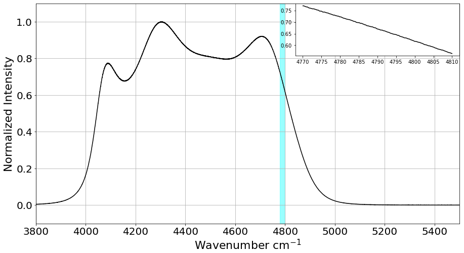
An example of a spectral fit is shown in Fig. 1 where we can observe how the measured spectra fit the calculated spectrum. On the left, at wavenumbers lower than 4794 cm⁻¹, there is an overlap between measured transmittance (Tm) and CO₂. However, after that, at higher wavenumbers, the measured spectrum slopes down and we can see a considerable gap between it and the CO₂ lines towards the end of the window. This is caused by the filter used to record this spectrum. The w4790 window is located near the end of the filter 4433, where the transmission has started to decline (see Appendix C).

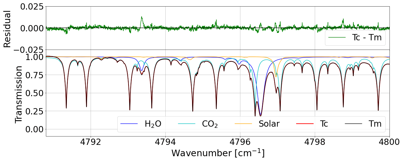
Figure 1 An example of the computed transmittance (Tc) and the measured transmittance (Tm) for the w4790 window, CO₂ absorption lines, and other gases, as well as the residual (Tm − Tc) for a typical InSb spectrum acquired in Ny-Ålesund.

To provide the best fit to the measured spectrum and minimize the residuals, other gas profiles and other parameters are scaled and adjusted. The gas mole fraction is retrieved from these scaled profiles (Wunch et al., 2015). The parameters fitted are continuum level, continuum tilt, continuum curvature, frequency shift, and solar lines. The gases fitted are CO₂, H₂O, HDO, CH₄, and N₂O. See Appendix A for the full window fitting parameters used in the retrieval.

For comparison the TCCON xCO₂ data from Ny-Ålesund (Buschmann et al., 2022) and Burgos (Morino et al., 2022) were used. These windows are centered at 6220.00 and 6339.50 cm⁻¹ with spectral widths of 80 and 85 cm⁻¹, respectively (Wunch et al., 2011a). Additionally, TCCON is introducing a new window in the 4800 cm⁻¹ region called lCO₂; for more details refer to Appendix G.

Table 1 The names of the three different xCO₂ retrievals, with the spectral details, the resolution of each spectra used, and the data availability for each site.

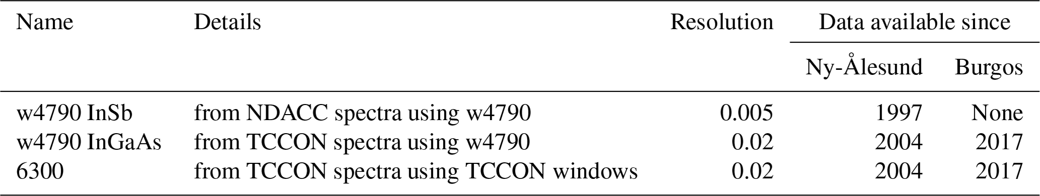
In this study we work with two types of spectra that we will denote with the detector used to record: InGaAs and InSb. Following this, we have three windows used for retrievals: the w4790 and the two TCCON windows around 6300 cm⁻¹. Details of the three xCO₂ retrievals are shown in Table 1.

2.3 Retrieval method

The retrieved xCO₂ in this study is obtained by the profile scaling algorithm GFIT (version 5.28 in GGG2020) nonlinear least-squares fitting algorithm, which is also used for the TCCON xCO₂ retrievals. A full description is available in Laughner et al. (2020).

The CO₂ column-averaged dry-air mole fraction (DMF) retrieved by TCCON is calculated using CO₂ obtained from the band at 7885 cm⁻¹. The well-mixed CO₂ is used to estimate the total dry-air column. The column-averaged dry-air mole fraction is derived by dividing the vertical column (VC) of CO₂ by the VC of O₂ (Wunch et al., 2011a). For the purpose of this retrieval the O₂ mole fraction is assumed to be constant.

$$\begin{array}{}\text{(1)}& {\mathrm{xCO}}_{\mathrm{2}}={\displaystyle \frac{{\mathrm{VC}}_{{\mathrm{CO}}_{\mathrm{2}}}}{{\mathrm{VC}}_{{\mathrm{O}}_{\mathrm{2}}}}}\times \mathrm{0.2095}\end{array}$$

w4790 xCO₂ was also retrieved using the GFIT software for both InSb and InGaAs spectra. However, InSb spectra used here do not contain an O₂ window. An additional difference between the w4790 window and the 6300 TCCON windows is that we do not currently apply an air-mass-dependent correction (ADCF) or in situ correction factor (AICF) to the w4790 xCO₂, while the TCCON xCO₂ includes both. The mole fraction for the MIR spectra was calculated using the dry-air column abundance inferred from the surface pressure (Wunch et al., 2011a) with the following equation.

$$\begin{array}{}\text{(2)}& {\mathrm{xCO}}_{\mathrm{2}}={\displaystyle \frac{{\mathrm{VC}}_{{\mathrm{CO}}_{\mathrm{2}}}}{\frac{P_{\mathrm{s}}{N}_{\mathrm{A}}}{m_{\mathrm{air}}^{\mathrm{dry}}\mathit{\left\{}g\mathit{\right\}}}-\frac{{\mathrm{VC}}_{{\mathrm{H}}_{\mathrm{2}}\mathrm{O}}{m}_{{\mathrm{H}}_{\mathrm{2}}\mathrm{O}}}{m_{\mathrm{air}}^{\mathrm{dry}}}}}\end{array}$$

VC${}_{{\mathrm{CO}}_{\mathrm{2}}}$ is the CO₂ vertical column from the GGG2020 output from w4790, VC${}_{{\mathrm{H}}_{\mathrm{2}}\mathrm{O}}$ is the vertical column from the GGG2020 output for water vapor from the window at 4576.85 cm⁻¹ of width 1.90 cm⁻¹, P_s is the surface pressure (hPa), $N_{\mathrm{A}}=\mathrm{6.0221415}\times {\mathrm{10}}^{\mathrm{23}}$ molec. mole⁻¹ is the Avogadro number, $m_{\mathrm{air}}^{\mathrm{dry}}=\mathrm{28.9644}$ g mole⁻¹ is the mass of dry air, $m_{{\mathrm{H}}_{\mathrm{2}}\mathrm{O}}=\mathrm{18.01534}$ g mole⁻¹ is the mass of water, and the column-averaged gravitational acceleration is {g}=9.81 m s⁻².

These are two main important differences between the 6300 and the w4790 retrievals: the calculation of the mole fraction using CO₂ or pressure and the inclusion of an air mass and in situ correction or lack thereof (the two corrections are explained in Sect. 4.2 and 4.4, respectively).

The retrieved mole fraction is quality-controlled following flagging similar to TCCON (Wunch et al., 2011a). Data points with high solar zenith angles (SZAs) (> 83^∘ as used by TCCON in Burgos) and/or high relative retrieval errors (10 % of the average) were discarded; spectra with negative error output were also removed. Finally, data points with high relative retrieval error (> 20 % of the average) of H₂O were filtered out.

For the time series, an error-weighted daily mean (${\stackrel{\mathrm{‾}}{x}}^{\mathrm{daily}}$) and the standard deviation of the daily mean (σ_w4790) were calculated. Because InSb spectra recorded each day on the filter covering w4790 are not abundant (usually less than 20 spectra per day), the weighted daily mean of 6300 was used to calculate the standard deviation.

$$\begin{array}{}\text{(3)}& {\displaystyle }{\stackrel{\mathrm{‾}}{x}}^{\mathrm{daily}}={\displaystyle \frac{{\sum }_N^i\frac{x_i}{{\mathit{ϵ}}_i^{\mathrm{2}}}}{{\sum }_N^i\frac{\mathrm{1}}{{\mathit{ϵ}}_i^{\mathrm{2}}}}}\text{(4)}& {\displaystyle }{\mathit{\sigma }}_{\mathrm{w}\mathrm{4790}}=\sqrt{{\displaystyle \frac{{\sum }_N^i{\left(\frac{x_i-{\stackrel{\mathrm{‾}}{x}}^{\mathrm{daily}}}{{\mathit{ϵ}}_i}\right)}^{\mathrm{2}}}{{\sum }_N^i\frac{\mathrm{1}}{{\mathit{ϵ}}_i^{\mathrm{2}}}}}}\end{array}$$

Here, x_i is a given xCO₂ value and ϵ_i its corresponding relative retrieval error.

The error budget was approximated by using the standard deviations of the daily means (Eq. 4) and the standard error to better reflect the uncertainty in the daily mean, which is affected by the number of measurements. In addition, the diurnal variation was calculated to determine the precision following Yang et al. (2002).

$$\begin{array}{}\text{(5)}& \mathrm{DV}=\left({\displaystyle \frac{x}{{\stackrel{\mathrm{‾}}{x}}_{\mathrm{daily}}}}-\mathrm{1}\right)\times \mathrm{100}\end{array}$$

In the next sections several sensitivity tests and error budgets are presented to determine the quality of the retrieval.

3 Averaging kernels

In this section the effect of the different averaging kernels on the retrieved xCO₂ is evaluated by comparing two different retrievals (Rodgers and Connor, 2003). For a perfect column measurement, the column averaging kernel should be 1.0 at all altitudes, but in practice, there is greater sensitivity to some altitudes than others. The column averaging kernels depend on the retrieval method and the choice of parameters to be fitted as well as the solar zenith angle (Wunch et al., 2011a). The main difference in the averaging kernels originates in the shape and depth of the absorption lines. In this case the w4790 InSb CO₂ averaging kernels show high sensitivity in the troposphere, and it decreases towards the upper atmosphere. High sensitivity remains towards the stratosphere because the lines used are weak and do not saturate.

In Fig. 2 we see the averaging kernels for w4790 InGaAs in Ny-Ålesund, and those corresponding to w4790 InSb spectra look very similar (see Fig. I1 in the Appendix).

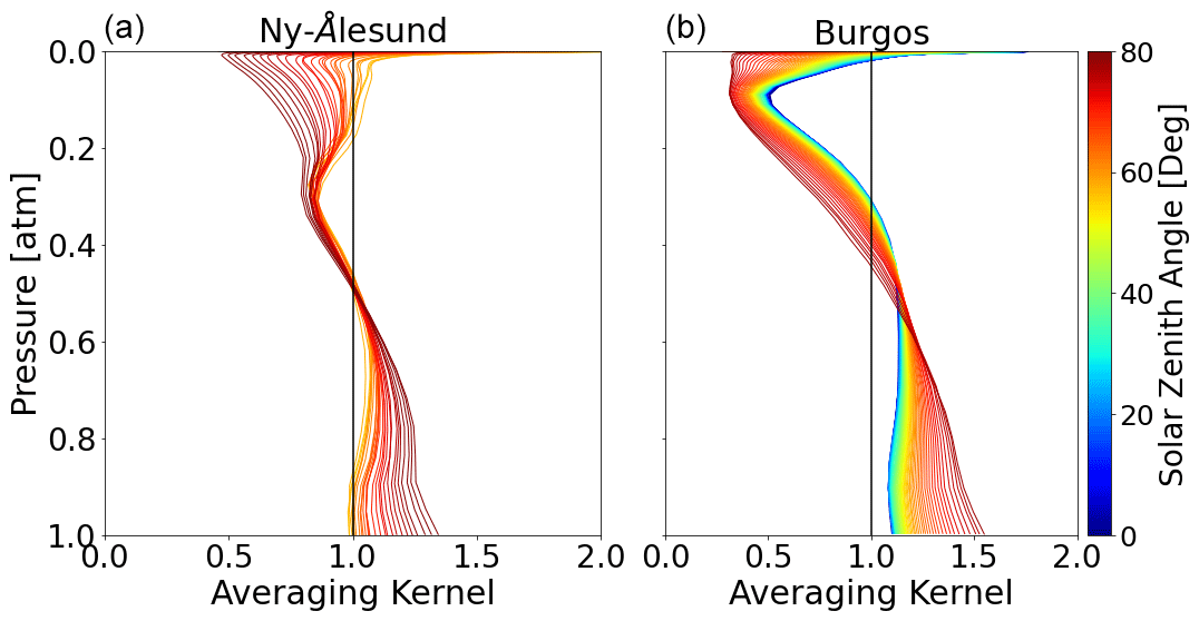
Figure 2 The w4790 averaging kernels averaged to 1^∘ for InGaAs Ny-Ålesund on the left and Burgos on the right.

We observe that the averaging kernels for Burgos look different to Ny-Ålesund; however, they follow a similar shape but with the minimum lying at different altitudes. When seeing the averaging kernels plotted against altitude (see in Figs. I3 and I4 in the Appendix) the overall shape is similar but the minimum occurs around 10 km for Ny-Ålesund and around 15 km in Burgos, and the maximum is between 40 and 50 km for both. This is probably due to the difference in the height of the tropopause in both locations, Burgos having a higher tropopause than Ny-Ålesund.

4 Sensitivity studies

4.1 A priori influence

As described by Rodgers (2000), the retrieved quantity $\widehat{\mathit{x}}$​​​​​​​ relates to the true atmospheric quantity x, the a priori x_a, and the averaging kernel A by the following equation:

$$\begin{array}{}\text{(6)}& \widehat{\mathit{x}}-{\mathit{x}}_{\mathrm{a}}=\mathbf{A}\left(\mathit{x}-{\mathit{x}}_{\mathrm{a}}\right)+{\mathit{ϵ}}_x,\end{array}$$

where ϵ_x is the random and systematic error term. The a priori profile will influence the retrieved xCO₂ depending on how much the measured information can constrain the retrieval (Rodgers, 2000). The prior profiles of GGG2020 are produced using the Goddard Earth Observing System Forward Product for Instrument Teams (GEOS-5 FP-IT or GEOS FP-IT) (Lucchesi, 2015) reanalysis product that has a temporal resolution of 3 h. The full description is found in Laughner et al. (2023a).

The use of a priori profiles that are close to the true atmosphere can give the impression of a successful retrieval, even if the information content of the measured quantity is not sufficient. To avoid this possibility, the influence of the a priori needs to be evaluated with a test retrieval performed with a modified a priori, as shown in this section. The modified a priori is initially fixed to 400 ppm at all altitudes and includes a linear increase of 0.1 ppm for each modeled profile (see Fig. I5 in the Appendix). The xCO₂ retrieved using the modified a priori is then compared to the xCO₂ retrieved using the standard a priori. Apart from the different a priori, the same retrieval algorithm, procedure, and post-processing parameters have been used as in the original retrievals with the standard a priori.

For both locations, the correlation coefficients R² between the retrievals with the fixed and the standard a priori are better than 0.95, which means a strong correlation. From Fig. 3 we observe that the scattering for Burgos is higher than for Ny-Ålesund, likely due to the higher humidity and temperature given that the window is temperature-sensitive. For Ny-Ålesund we see in the latest years a tendency to shift towards lower ΔxCO₂. The modified a priori used for these tests includes a linear increase in xCO₂. This increase might not correctly represent the atmospheric evolution and result in an overestimation. For both locations, the ΔxCO₂ is mostly smaller than 2 ppm.

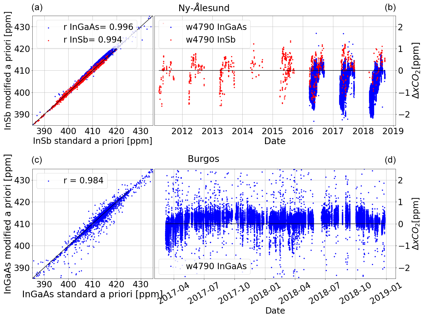
Figure 3 (a, b) Ny-Ålesund InGaAs (2016–2018) in blue and InSb (2012–2018) in red. (c, d) Burgos (2017–2018). (a, c) The correlation plots and (b, d) the difference between xCO₂ retrieved with the standard a priori minus the xCO₂ retrieved with the modified a priori, ΔxCO₂.

4.2 Solar zenith angle dependence

The w4790 xCO₂ has an air-mass-dependent artifact and an air-mass-independent artifact, similar to the TCCON xCO₂. The air-mass-dependent artifacts are primarily caused by systematic errors introduced by spectroscopic inadequacies in the line list and instrumental problems (Wunch et al., 2011a).

From Wunch et al. (2011a), the TCCON xCO₂ product has an SZA or air-mass-dependent artifact causing the retrieval to be larger by approximately 1 % at 20^∘ SZA than at 80^∘ SZA. To correct this, TCCON applies an empirical correction (ADCF). In GGG2014, the correction was derived separately for each xGAS product. In GGG2020, it is derived for each retrieval window.

In this study we did not apply the air mass correction (ADCF) to the w4790 retrievals shown to determine if the retrieval of xCO₂ has to be corrected for air mass artifacts. We show in Fig. 4 $x{\mathrm{CO}}_{\mathrm{2}}-\stackrel{\mathrm{‾}}{x}{\mathrm{CO}}_{\mathrm{2}}$ against SZA, where $\stackrel{\mathrm{‾}}{x}{\mathrm{CO}}_{\mathrm{2}}$ is the daily mean. Under the assumption that, on a given day, any variation of xCO₂ that is symmetrical around noon is an artifact and anti-symmetrical variations are real, the dependence on the SZA is observed (Wunch et al., 2011a).

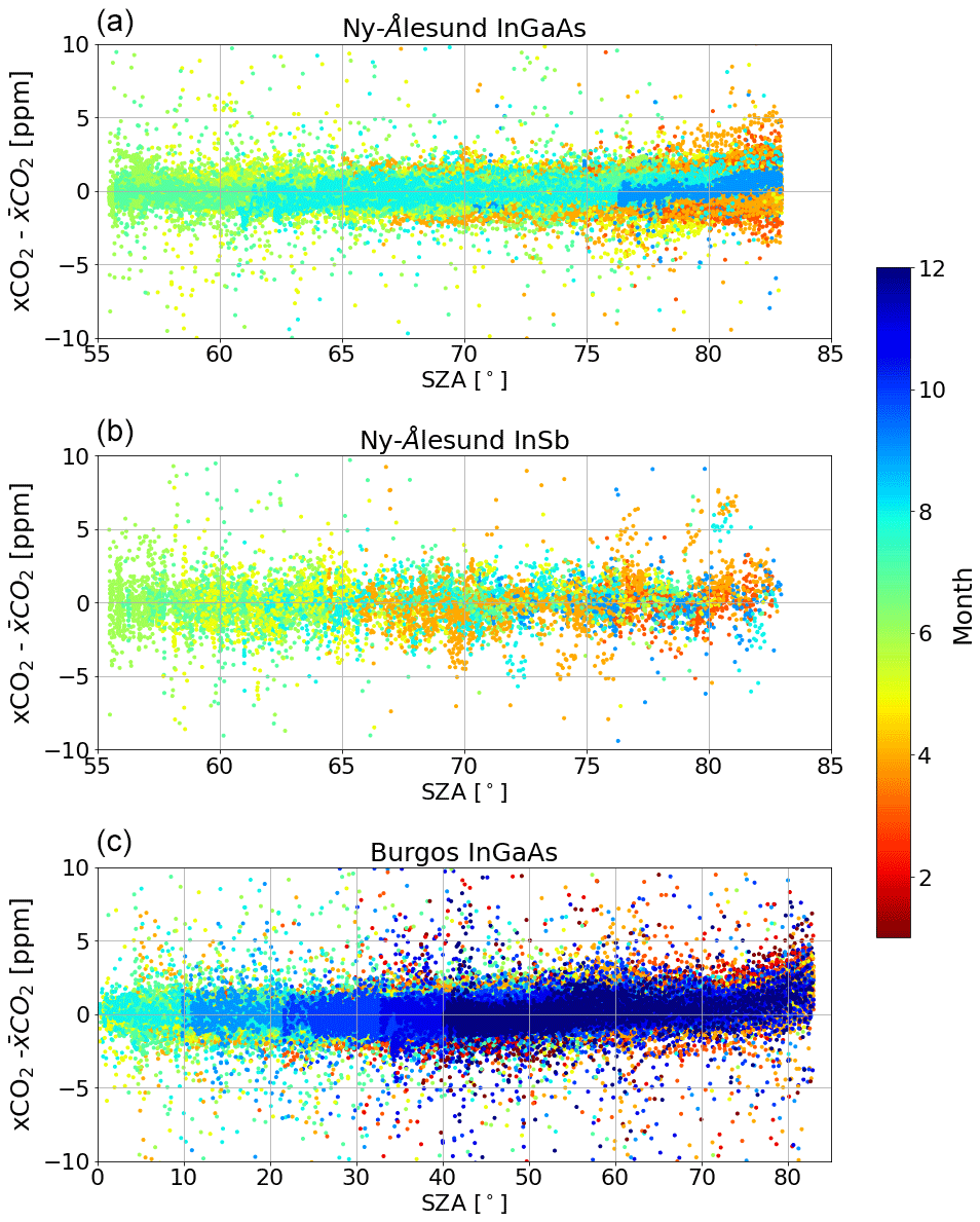
Figure 4 (a) Ny-Ålesund w4790 InGaAs (2016–2018) xCO₂ minus the daily mean. (b) Ny-Ålesund w4790 InSb (1997–2018) xCO₂ minus the daily mean. (c) Burgos w4790 InGaAs (2017–2018) xCO₂ minus the daily mean.

For w4790 InGaAs, we can see that there is an increase in the scattering of xCO₂ at SZA larger than 75^∘ for Ny-Ålesund. Some values can be approximately 1 % larger at 83^∘ than at SZA lower than 75^∘, and others remain within the range ±2 ppm. w4790 InSb seems to remain mostly unchanged for the SZA range (50 to 83^∘), but there is the possibility that this is due to the low number of data points.

For Burgos there is an increase in all xCO₂ values for SZA larger than 50^∘, with values around 83^∘ being 1 % larger than for SZA values below 50^∘. This asymmetry around zero indicates an air mass dependence for large SZA. On the other hand, we found that for the 6300 window, prior to the air mass correction, the tendency is consistent with the findings of Wunch et al. (2011a) where at lower SZA the values are higher than at high SZA (see Figs. I6 and I7 in the Appendix). This indicates that both retrievals have an air mass dependence, especially for high SZA, but the observed artifacts are different.

4.3 Site-to-site consistency

This section serves to investigate if the scaling between 6300 and w4790 xCO₂ is consistent between locations. To emulate a correction via a scaling factor, a ratio between 6300 and w4790 for each data point was calculated.

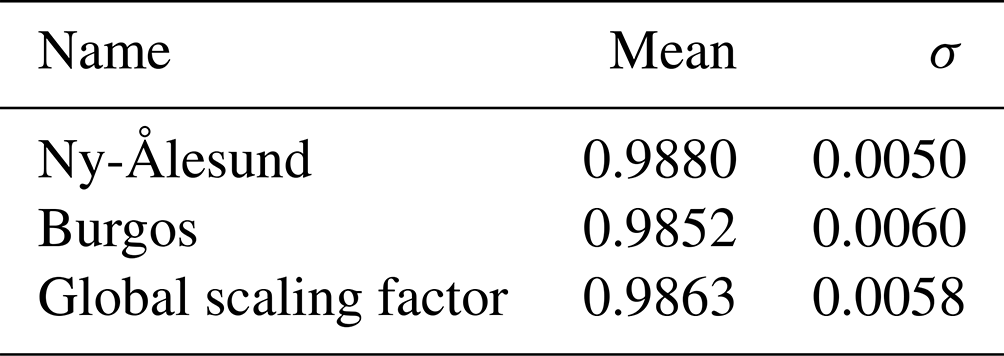
The means of the ratios (shown in Fig. 5) were calculated with their corresponding standard deviation; these values are presented in Table 2. The difference between the ratios' means are within the error, indicating good consistency between the two sites. These values also serve to determine the global scaling factor (GSF) to be applied to both w4790 retrievals shown in Sect. 7. To determine a global SF, all data points from Ny-Ålesund and Burgos were used to calculate the mean. Table 2 shows the values for the ratios and the SF.

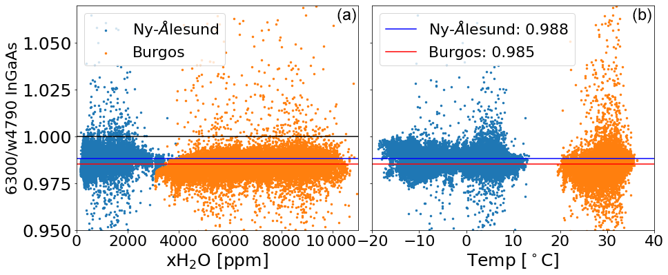
Figure 5 The ratios (6300 xCO₂ $/$ w4790 InGaAs xCO₂) of Ny-Ålesund (2016–2018) are in blue and Burgos (2017–2018) are in orange plotted against (a) xH₂O and against (b) temperature. The means of the ratio are presented as lines: blue for Ny-Ålesund and red for Burgos.

Table 2 The means of the ratios and corresponding standard deviations between w4790 and InGaAs 6300.

4.4 Comparison with aircraft profiles

The air-mass-independent correction factor (AICF) (also called in situ correction) is determined with collocated in situ profiles. The procedure for this comparison is similar to the calibration of TCCON described in Wunch et al. (2010). We also check for correlation between the TCCON–in situ difference and both xluft and SZA (See Fig. I8). xluft is used to diagnose instrument or retrieval errors and is calculated as a ratio of two columns of dry air (one derived from surface pressure and the prior H₂O profile and the second derived from the retrieved O₂ column). We use this correlation to check how sensitive the w4790 window is to instrument errors. Similarly, we use the correlation with SZA to check whether the air mass correction for this window is likely to be significant.

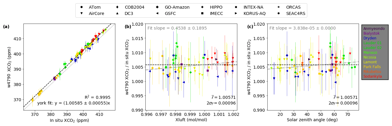
Figure 6 (a) Correlation between w4790 xCO₂ and in situ xCO₂. (b) Ratio of w4790 xCO₂ window to in situ xCO₂ against xluft between 0.996 and 1.002. (c) Ratio of w4790 xCO₂ window to in situ xCO₂ against solar zenith angle.

The correlation between w4790 xCO₂ and in situ xCO₂ in Fig. 6a shows a good performance of w4790 at the sites evaluated. The correlation coefficient R² is 0.9995.

The w4790 has a slightly larger scatter and stronger relationship between xluft and the bias vs. in situ xCO₂ than the TCCON 6300 windows. This means that if xluft deviates much from the nominal 0.999 value, there will be an increased bias in xCO₂ (see Fig. 6b). There is a weak correlation between the bias and the SZA (see Fig. 6c). The variation with SZA is smaller than the scattering; therefore, the lack of air mass correction is a minor component. The higher scatter is to be expected as the w4790 has higher sensitivity towards the surface, and this might be driven by the surface variability of CO₂ that aircraft and balloons cannot capture, in addition to the temperature sensitivity of the window. These features make the w4790 single data point uncertainties larger than those of 6300.

The mean ratio between w4790 xCO₂ and in situ xCO₂ is 1.01 for the 6300 windows and 1.005 for w4790 window, suggesting that the line strengths in the 6300 windows are biased lower than in the w4790. For the 6300 window, this bias is removed by the in situ correction. Likewise, we will similarly apply an in situ correction for the w4790 derived from this analysis. Additionally, while the correlation between the bias and SZA in Fig. 6 (right) is small, we will derive an air-mass-dependent correction factor for the w4790 xCO₂ in the future to remove this small dependence.

5 Error analysis

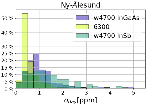
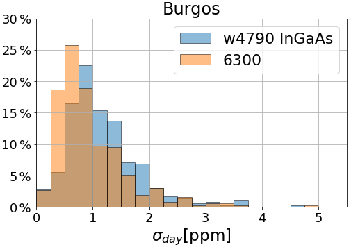
In this section we will look into the systematic and random errors of this retrieval. This analysis was performed on filtered data as described in Sect. 2.3. A total of 3304 data points for InGaAs were flagged and removed, leaving 46 307 usable points. For InSb 121 data points were flagged and removed, leaving 1115 usable data points. In total, less than 10 % of the original data points were filtered out.

As described by Eq. (4), an error-weighted standard deviation of the daily mean, σ_day, was calculated for the years presented in the previous sections. To evaluate the distribution of σ_day, we will list the values below which we find 95 % of σ_day (2 standard deviations) for each location and retrieval. For 6300, 95 % of σ_day is below 1.5 ppm for Ny-Ålesund and below 2 ppm for Burgos. For w4790 InGaAs, over 95 % of the error σ_day is below 2 ppm for both locations. For w4790 Insb, around 95 % is below 2.75 ppm. The σ_day is larger for w4790 InSb, but one thing to consider is the difference in the number of data points between InSb and InGaAs that affects the standard deviation. For this reason the standard error was also calculated (shown in Table 3) to have a representation of mean error.

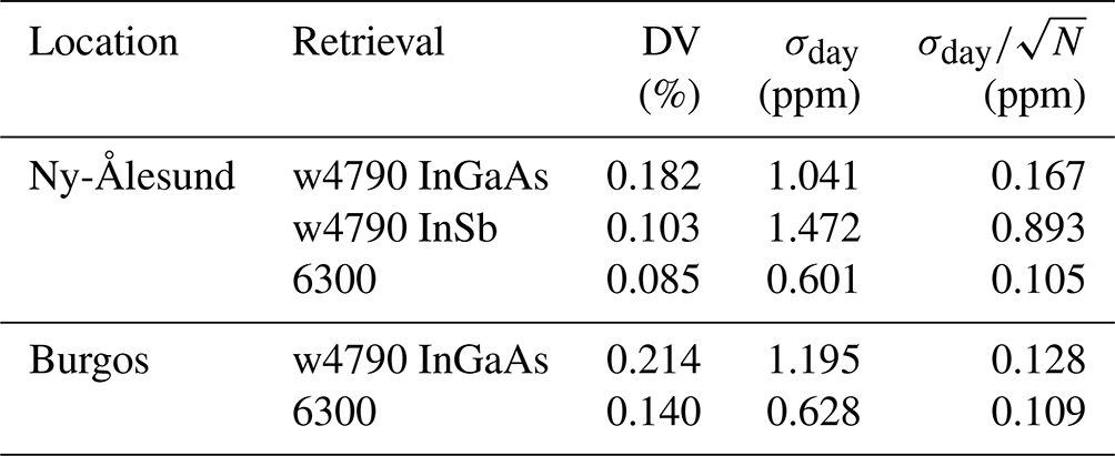
Table 3 Estimated errors for the retrievals, the mean of the absolute value of the diurnal variation (DV), the mean standard deviation (σ), and the standard error ($\mathit{\sigma }/\sqrt{N}$) of the daily means of Burgos (2017 and 2018) and Ny-Ålesund (2016–2018).

5.1 Diurnal variations

The precision of the column-averaged dry-air mole fraction is estimated from its diurnal variation (Yang et al., 2002); see Eq. (5) for a definition. Part of the diurnal variation (DV) is caused by real variations in the atmospheric xCO₂, dependent on the local natural diurnal cycles, while the other part is composed of errors; therefore, this method gives an upper limit for the precision. However, this strategy was still chosen as, due to the small number of data points of InSb spectra, it is a shorter time period in which to make a meaningful average.

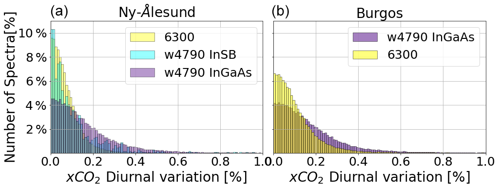
The diurnal variations follow a similar pattern for all InGaAs retrievals, following a normal distribution (compare Fig. 7). However, w4790 InSb looks different than the rest. For w4790 InGaAs, 95 % of the diurnal variations are below 0.384 % in Ny-Ålesund and 0.425 % in Burgos, while for w4790 InSb 95 % is below 0.246 %. The fewer data points measured per day for InSb might explain why the DV extends to 1 %. There is a total of fewer than 500 data points for the 3 years for InSb, while there are over 4600 InGaAs data points for the same 3 years. For 6300, 95 % of the diurnal variations are below 0.103 % in Ny-Ålesund and 0.247 % in Burgos. As we saw in Sect. 5, the retrievals for w4790 have more scattering than 6300; this can be seen in the diurnal variation as well.

Figure 7 Histograms of the diurnal variations in Ny-Ålesund (a) and Burgos (b).​​​​​​​

5.2 Perturbations of potential error sources

This subsection presents a sensitivity study of the w4790 xCO₂ retrieval, where several retrieval input parameters were perturbed by a realistic amount following a similar method to Wunch et al. (2011a). For the InGaAs tests, Burgos spectra were used, and for the InSb tests, Ny-Ålesund spectra were used. The quantities are listed in Table 4 followed by the average of each of the perturbations for each site. All tests, except for the CO₂ a priori profile, were performed with positive and negative perturbations (i.e., +5 and −5 s); this is to evaluate if they behave in a symmetric way.

Table 4 The w4790 error budget; in the first column is the error source, and the second column is the magnitude of the perturbation. The last two columns are the average magnitudes of the fractional difference (FD) per perturbation of the retrieved xCO₂ for Ny-Ålesund and Burgos.

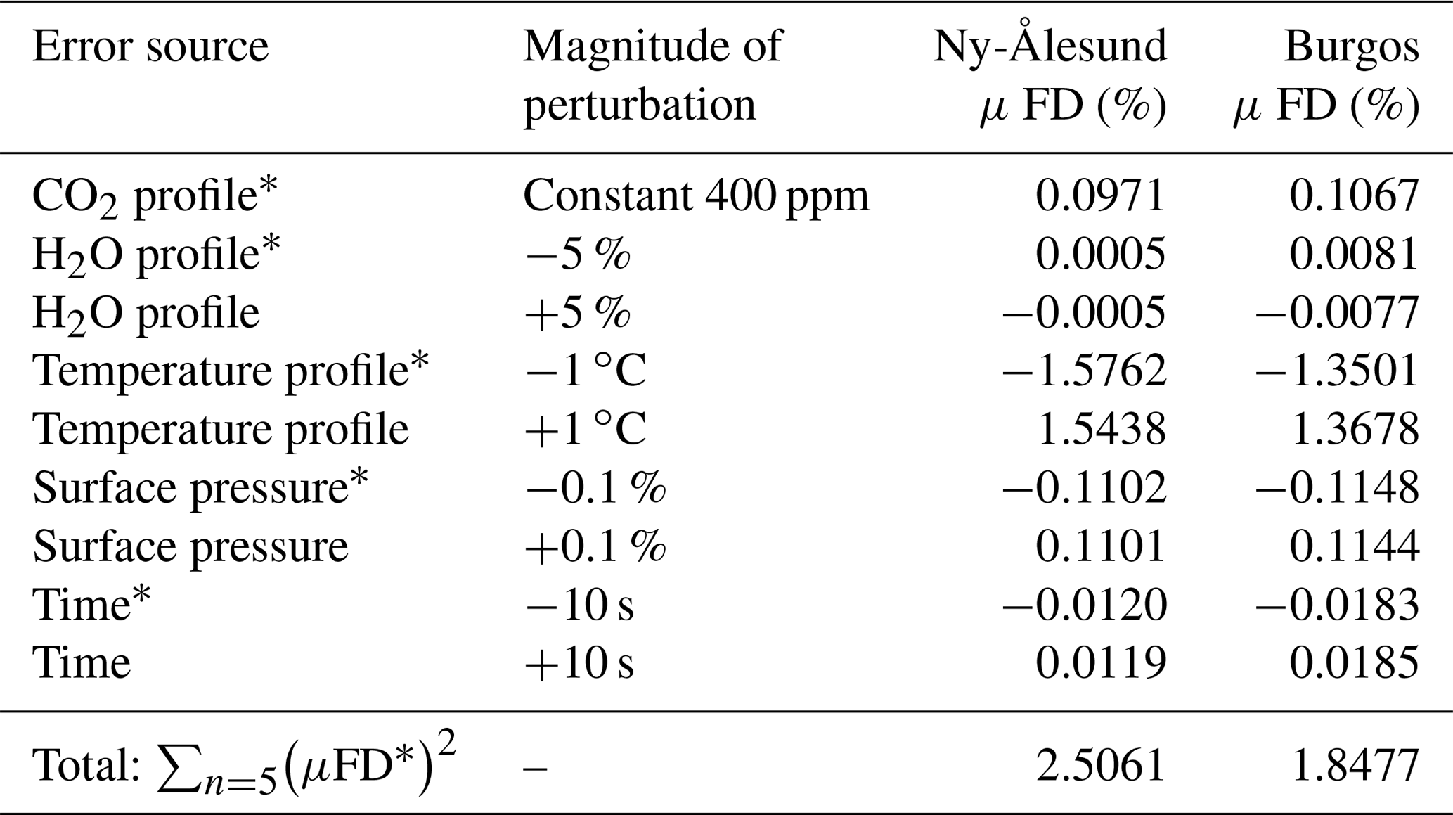
^∗ Corresponds to the perturbations used for the calculation of the total sum of the squared errors from these sources as similarly performed in Wunch et al. (2011a).

The perturbations were performed by slightly modifying variables in different retrieval steps. Two perturbations were done by multiplying by, adding to, or subtracting from the whole profile in the a priori input files. The H₂O profile was multiplied by 1.05 or 0.95, and for the temperature profile ±1 ^∘C was added. The CO₂ perturbation was done by replacing the a priori profile with 400 ppm for all layers. For pressure, the measured surface pressure was multiplied by 1.0001 or 0.9999. Lastly, time of measurement was perturbed by adding ±10 s. Then the output of each perturbed retrieval was evaluated against the unperturbed case by calculating the fractional difference (FD) with the following formula:

$$\begin{array}{}\text{(7)}& \mathrm{FD}=\mathrm{100}\times \left({{\mathrm{xCO}}_{\mathrm{2}}}^{\mathrm{unp}}-{{\mathrm{xCO}}_{\mathrm{2}}}^{\mathrm{p}}\right)/{\mathrm{xCO}}_{\mathrm{2}}^{\mathrm{unp}},\end{array}$$

where ${{\mathrm{xCO}}_{\mathrm{2}}}^{\mathrm{unp}}$ is the unperturbed total column and ${{\mathrm{xCO}}_{\mathrm{2}}}^{\mathrm{p}}$ is the perturbed total column. The results are shown in Fig. 8.

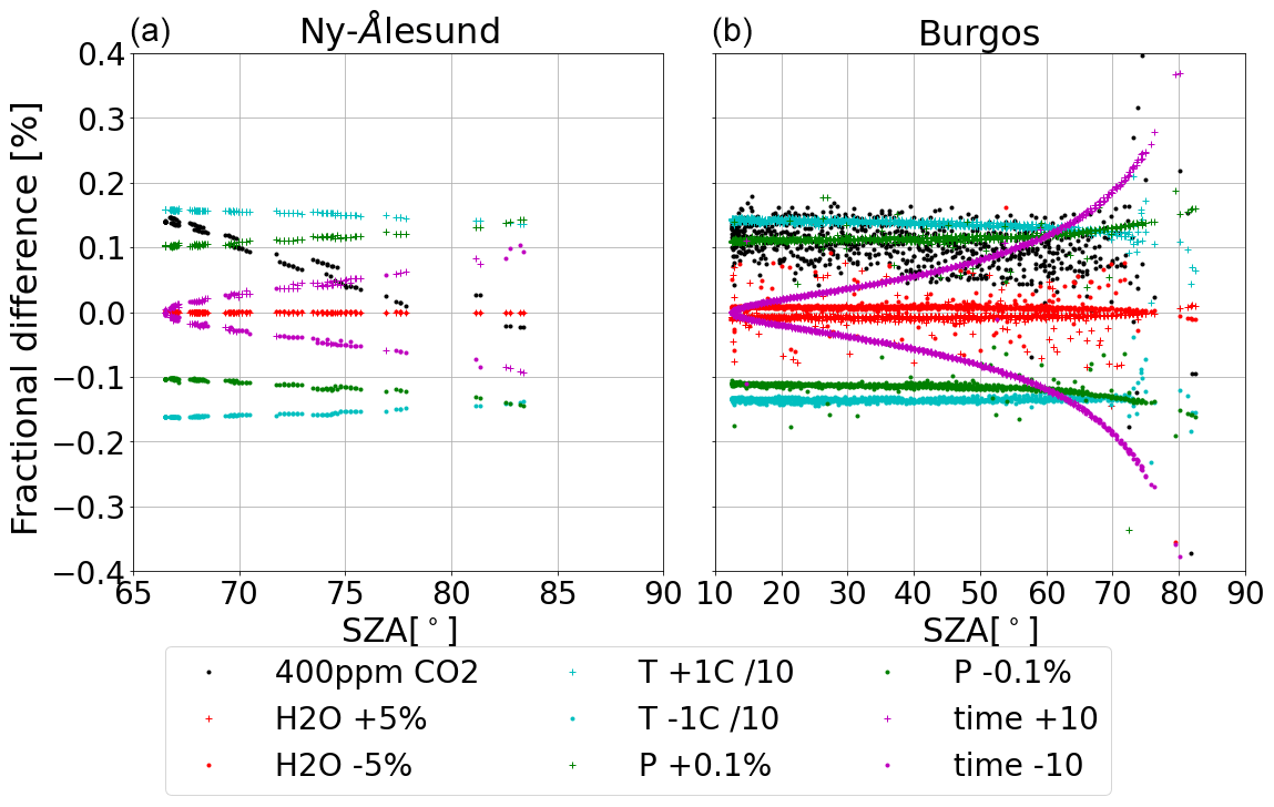
Figure 8 Fractional difference of perturbations (CO₂ a priori profile, H₂O a priori profile, surface pressure, time, and temperature a priori profile divided by 10) as a percent of the retrieved CO₂ for Ny-Ålesund (InSb, a) and Burgos (InGaAs, b). Remark: the values for the temperature perturbations are divided by 10 to fit in the plot range.​​​​​​​

The w4790 retrieval is more sensitive to pressure perturbations than TCCON, which is expected, as it makes use of pressure in the calculation of the dry-air mole fraction. For TCCON the pressure error (−0.1 % profile perturbation) is −0.036 at SZA 20^∘ and −0.033 at SZA 70^∘ (Wunch et al., 2011a). From Wunch et al. (2011a) we know that the largest errors for xCO₂ computed using surface pressure are zero-level offsets, surface pressure errors, and Sun tracker pointing errors and that those are larger compared to using CO₂ $/$ O₂. This is consistent with the findings of the perturbation tests performed for this study.

Along with pressure, as mentioned in previous sections, the temperature sensitivity of w4790 is also an important source of error. The Ny-Ålesund and Burgos temperature perturbations behave symmetrically and are the largest source of error. The negative perturbation mean is −1.5 % K⁻¹, and the positive perturbation mean is 1.5 % K⁻¹.

The time perturbations have both positive and negative effects depending on the time of the day. For the +10 s case, the effect is a negative bias in the morning and a positive error in the afternoon. The opposite happens in the −10 s case. Both intersect at the zero line at the minimum SZA of the day. This behavior was expected due to the nature of the SZA and time corrections observed in spectroscopy gas retrievals. The results of the perturbations of pressure and H₂O that have both positive and negative magnitudes behave symmetrically. For pressure, a perturbation of +0.1 % generates a negative difference in the xCO₂ retrieval of approximately −0.1 % and vice versa for both Burgos and Ny-Ålesund. For H₂O, the smallest of all perturbations, a positive perturbation also causes a negative difference in the xCO₂ retrieval. However, the magnitude of the difference is larger in Burgos than in Ny-Ålesund. This is to be expected, given that the atmospheric water content in Burgos is larger.

For the perturbations of the xCO₂ a priori profile, we have a different effect in both locations. For Burgos, a constant a priori causes an offset of less than 0.1 %. But for Ny-Ålesund, the effect is SZA-dependent, having the largest difference (−0.122 %) at the largest SZA during the morning. Then it decreases, crossing zero at 65^∘, and at midday, when the SZA is the smallest (∼ 60^∘), the difference is positive (∼ 0.05 %). Finally, at the end of the day, the difference is negative once again.

The total average error caused by all four sources is calculated by adding the square of the mean of the negative perturbations (denoted by * in Table 4), resulting in 2.5 % for Ny-Ålesund and −1.8 % for Burgos.

6 xCO₂ time series

In this section the time series is presented for historical data in Ny-Ålesund from 1997 to 2018. There are some spectra that have been recorded since 1992; however, the specific filter used was installed later. The full retrieved time series of xCO₂ can be seen in Fig. 12.

The data were processed, filtered, and scaled, and the daily mean was calculated for all three retrievals. Comparing the w4790 xCO₂ to the 6300 xCO₂ for the overlapping time will show how well the seasonality is represented as well as the scattering in comparison to the 6300 window.

We can see that the xCO₂ retrieved from w4790 can reproduce the seasonal cycle with the same amplitude of 10 ppm successfully. However, the w4790 xCO₂ data points show more scattering than the 6300 xCO₂; this is due to the influence of the averaging kernels as is addressed in the Appendix.

In Ny-Ålesund the recorded data cover March to October. During this period the solar zenith angle range changes. At the peak of summer the smallest SZA is around 55^∘, and during March and October the smallest SZA is around 73^∘. This means a difference in the minimum SZA of 18^∘. Given that the maximum SZA in the datasets is 83^∘, the range of SZA during spring and autumn is quite limited. We observe in Fig. 9 that the difference between w4790 InGaAs and 6300 changes during the year, being higher for spring and autumn than for the peak of summer. Taking into account Sect. 4.2 and the lack of air mass correction for both datasets, the changes in the range of the solar zenith angle can be responsible for this observed characteristic. The mean of the difference between w4790 InGaAs and 6300 is −0.895 ppm with a standard deviation of 1.513 ppm. The mean of the difference between w4790 InSb and 6300 is −0.620 ppm with a standard deviation of 1.516 ppm.

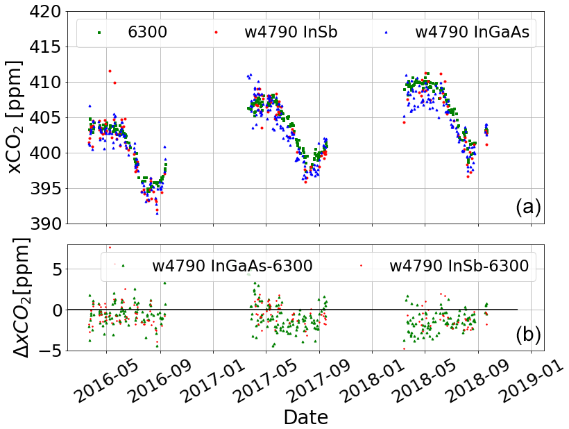
Figure 9 Ny-Ålesund weighted daily mean of w4790 InGaAs (blue triangles) and w4790 InSb (red dots) xCO₂ compared with the daily means of 6300 (green squares) xCO₂ for the overlapping years. (b) The difference between w4790 InGaAs and 6300 (green triangles) and between Insb and 6300 (red dots).

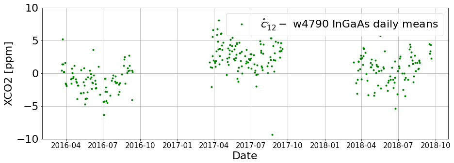
In Burgos, the seasonal cycle includes a dry (October to May) and a rainy season. The behavior of its seasonality, unlike Ny-Ålesund's, cannot be fitted to a cosine curve. In Burgos, like in Ny-Ålesund, there is a change in SZA depending on the month, but it is larger. Around December the smallest SZA is around 40^∘, while for June it reaches 0^∘, resulting in a difference in the minimum SZA of 40^∘, which is twice that of Ny-Ålesund. This means the dry season contains data with a smaller range of SZA than the wet season. We can observe that the scattering is larger during the first 3 months of 2018, corresponding to the dry season. Lastly, the scattering of both w4790 and 6300 is larger for the last 2 months of 2018 (see Fig. 10). This is similar to what is observed in Ny-Ålesund, where periods with a smaller SZA range have a higher w4790 InGaAs 6300 difference. This can also be due to different sensitivity towards the surface and to thin clouds. The mean of the difference between w4790 InGaAs and 6300 is 0.456 ppm with a standard deviation of 1.014 ppm.

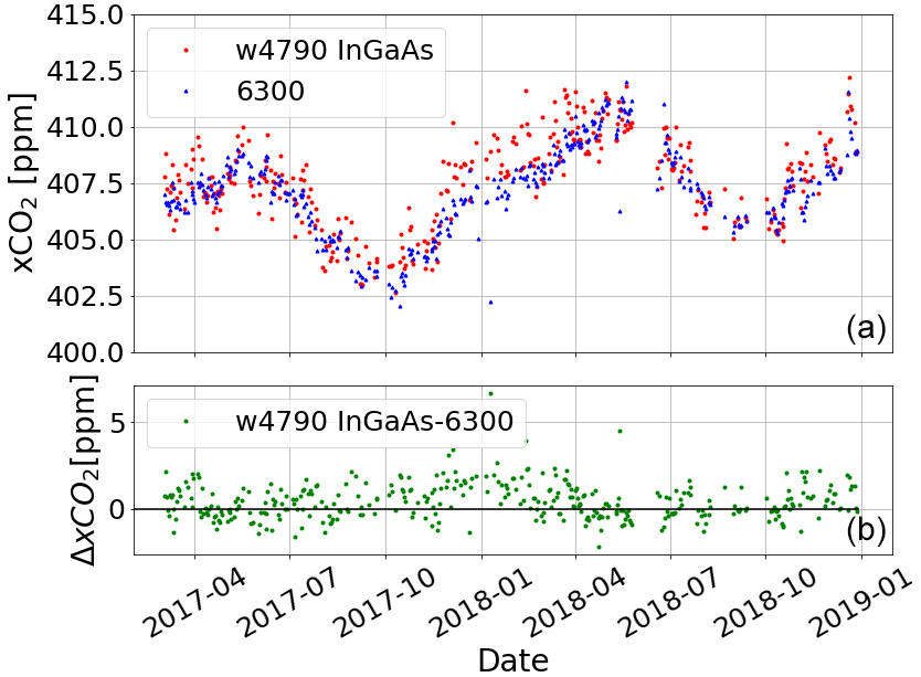
Figure 10 (a) Burgos weighted daily mean of w4790 InGaAs xCO₂ (red dots) compared with the daily means of 6300 xCO₂ (blue triangles) and the difference (in green) between them (b).

There are several InGaAs measurements per day performed for TCCON, while there are only a couple of InSb NDACC measurements per filter per day. This influences the scattering of the InSb data points to the fitted curve. There are several years in which there are very few data points or none. In 2005 and 1999 there were technical difficulties with the instrument; therefore, those years have one or no data points. The low number of measurements per year makes the InSb product very sensitive to thin clouds. All spectra with cloud contamination have been filtered out.

The correlation coefficients R² between the daily means of w4790 and 6300 (Fig. 11) are 0.934 for Ny-Ålesund InSb, 0.946 for Ny-Ålesund InGaAs, and 0.841 for Burgos.

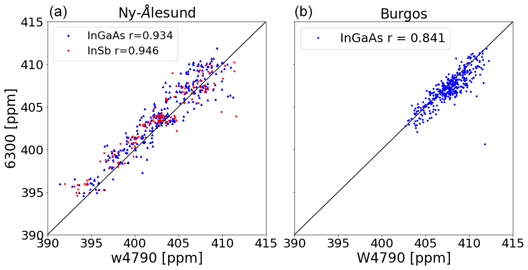
Figure 11 (a) The correlation between w4790 and 6300 xCO₂ for the overlapping years in Ny-Ålesund. In blue triangles represent w4790 InGaAs and 6300 xCO₂ daily means, and the red dots represent w4790 InSb and 6300 xCO₂ daily means. (b) The correlation between the weighted daily mean of w4790 InGaAs xCO₂ and the daily means of 6300 xCO₂ for Burgos.

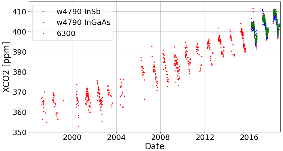
Figure 12 Ny-Ålesund weighted daily mean of w4790 InSb xCO₂ (red dots) for time series of all spectra available and the weighted daily mean of w4790 InGaAs (blue triangles) as well as the daily means of 6300 (green squares) for the 3 overlapping years.​​​​​​​

7 Retrieval strategy suggestion

Here we present setup recommendations for the acquisition of spectra to perform an xCO₂ retrieval from the 4800 cm⁻¹ region.

There are eight standard filters used by NDACC to acquire spectra in different regions (Blumenstock et al., 2021), but there are several other filters available for use. In Ny-Ålesund the nonstandard NDACC filter 4433 has been used since 1997, and in Bremen another nonstandard filter, 4825, that covers 4570 to 5080 cm⁻¹ is used. Both filters have a good transmission in the region of the w4790 window (see Appendix Figs. C3 and C4). For the 4433 filter the w4790 window is located near the end of the filter range but still above the 50 % cut-off. Both filters have been tested for the retrieval, and we can confidently recommend either.

Similarly to the protocols of NDACC, a KBr or CaF2 beam splitter that covers the spectral range can be used for acquisition (https://ndacc.larc.nasa.gov/data/protocols/appendix-ii-infrared-ftir, last access: 23 August 2023).

Different resolutions were tested with sample sets of InSb spectra measured in Bremen in March 2021 and used with the MIR xCO₂ retrieval. Lowering the resolution from 0.005 to 0.02 cm⁻¹ was found to have a negligible effect on the individual data points, while a larger number of measurements gives a higher temporal resolution and improves the precision of the retrieval as an average of more measurements reduces the noise. Lower resolutions did not show further benefit in terms of the precision, and very low resolution affects the retrieval as the spectral line shape is not resolved sufficiently. Furthermore, lower resolution allows for faster measurements and therefore more measurements, which allow better performance in cloudy conditions. Given that the retrieval works just as well at a TCCON resolution of 0.02 cm⁻¹ (OPD 45 cm), we recommend this resolution to increase the number of data points collected.

To keep temperature errors low the understanding and representation of the atmospheric temperature profile should improve (as seen in Sect. 5.2) and use data when a smoothed xluft mean is between 0.996 and 1.002 (as seen in Sect. 4.4). The input file where the spectral parameters to be fitted in GFIT are listed, known as the window file w4790.gnd, is shown in Appendix A.

8 Conclusions

This study showed that it is possible to successfully retrieve the column-averaged dry-air mole fraction xCO₂ from InSb NDACC spectra and from InGaAs TCCON spectra in the spectral window w4790. The averaging kernels show high sensitivity towards the surface. The retrieval proved not to have a big dependence on the a priori to correctly represent the daily and seasonal cycles (with correlation coefficients of at least 0.980 for all three retrievals). This is an improvement from Buschmann et al. (2016) where the averaging kernels limited the sensitivity, making the retrieval highly dependent on the a priori. The retrieval also proved useful to retrieve daily and subdaily values. However, the w4790 InGaAs and the 6300 xCO₂ both have an air mass dependence. For w4790 InGaAs, the values at larger SZA increase, while for 6300 they decrease. Additionally, w4790 retrievals are temperature-dependent and will require very accurate temperature measurements. Temperature is the largest error source with ±1.5 % K⁻¹, followed by pressure with ±0.11 % for ± 0.1 % error in the pressure measurement.

We showed that the xCO₂ product from w4790 InGaAs is site-consistent and has a global scaling factor (GSF) to the 6300 xCO₂ product of 0.9863 ± 0.0058 . That GSF was used for both time series and the corresponding correlations. The time series shown for the daily means show good agreement between 6300 and w4790 (InGaAs and InSb) with a larger scattering for w4790 caused by the influence of the averaging kernels (see the Appendix) and possible temperature inconsistencies.

The errors for w4790 retrievals are larger than 6300 for σ_day and $\frac{{\mathit{\sigma }}_{\mathrm{day}}}{\sqrt{N}}$ but of similar magnitude for the diurnal variation (DV). In agreement with the findings by Wunch et al. (2011a), the retrieval is most sensitive to pressure perturbations, which will require having well-calibrated pressure sensors. Implementing the new suggested setup for current and new NDACC measurement sites will provide valuable additional information on the carbon cycle.

Appendix A: The window fitting parameters

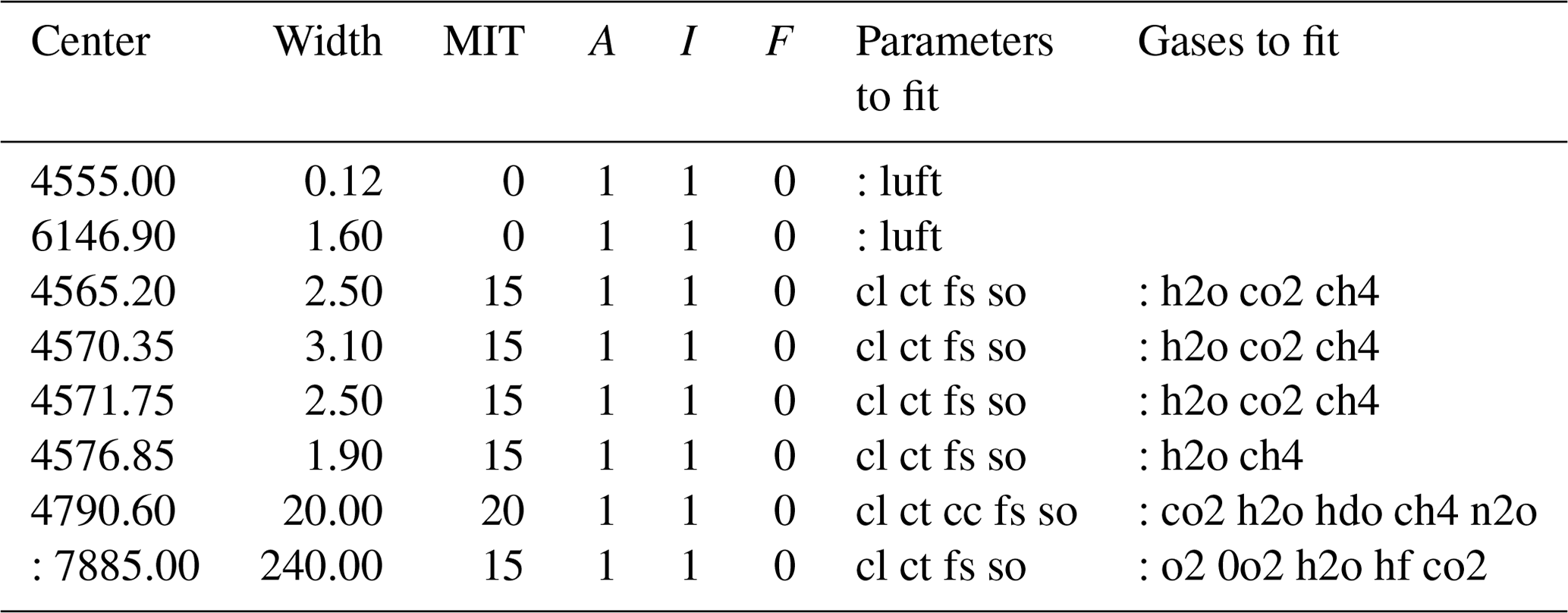
Table A1 These are the contents of the window file w4790.gnd used as input in the GFIT software specifying which windows will be used, their center and width, the gases to retrieve from each window, and other parameters. The O₂ line is commented out but can be used if the spectra include it. MIT is the maximum number of iterations, A is apodization, I is interpolation, and F is frequency reference frame (0: instrument, 1: Sun). The parameters to fit are as follows: cl is the continuum level, ct is continuum tilt, fs is frequency shift, “so” represents solar lines, and ak is used to generate the averaging kernels, which is an optional addition. The gases to fit are given, with the first species being the main species to fit and the following listing any interfering species to account for in the window.​​​​​​​

Appendix B: The effect of the averaging kernels

To evaluate how the averaging kernels (AKs) affect the retrieval a smoothing of the 6300 retrieval with the w4790 InSb averaging kernels was done. Using the 1^∘ SZA averaged AK, it was possible to interpolate to the exact solar zenith angle (SZA) of each of the spectra in 6300 and using Eq. (25) from Rodgers and Connor (2003) as done by Wunch et al. (2011b):

$$\begin{array}{}\text{(B1)}& {\widehat{c}}_{\mathrm{12}}^{\prime }=c_{\mathrm{c}}+\sum _j{h}_j{a}_{\mathrm{1}j}\left(\mathit{\gamma }{x}_{\mathrm{c}}-x_{\mathrm{c}}\right),\end{array}$$

where ${\widehat{c}}_{\mathrm{12}}^{\prime }$ is the smoothed total column, InSb = 1 and 6300 = 2, h_j is the pressure weighting, a represents the averaging kernels from the InSb spectra, and γ is the 6300 scaling factor applied to the a priori profile (x_c) to get the final 6300 profile that is then integrated to produce the total column ${\widehat{c}}_{\mathrm{2}}$ (Wunch et al., 2011b).

This comparison was chosen over using aircraft profiles due to availability. Aircraft profiles are scarce and do not cover a broad range of weather conditions or the variation with SZA. Hence, a comparison with aircraft would have been very limited.

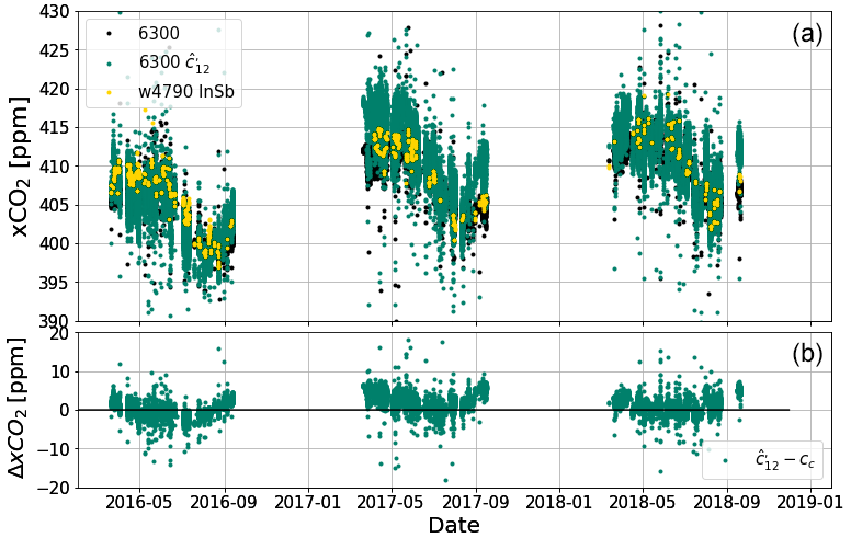
Figure B1 The comparison of xCO₂ from 6300 in black, the 6300 smoothed with the InSb averaging kernels in green, and the InSb w4790 in yellow. Panel (b) is the difference between the 6300 smoothed ${\widehat{c}}_{\mathrm{12}}^{\prime }$ and the 6300 xCO₂ ${\widehat{c}}_{\mathrm{2}}$.

Figure B2 The smoothed TCCON ${\widehat{c}}_{\mathrm{12}}^{\prime }$ daily mean minus w4790 InSb daily mean.

Figure B3 The smoothed TCCON ${\widehat{c}}_{\mathrm{12}}^{\prime }$ daily mean minus w4790 InGaAs daily mean.

Appendix C: The filters and their spectra

Here we show the measurement of solar spectra with each of the filters. The first is the NDACC 4433 used in Ny-Ålesund, and the second is the 4750 filter used in Bremen. The signal-to-noise ratio (SNR) for a single InGaAs spectrum in Ny-Ålesund is around 140 (calculated as an average of 21 March 2017 measurements), and in Bremen it is also around 140 (calculated as an average of 16 January 2020 measurements). The SNR for NDACC is 536.5 (derived from the residuum of the spectra in Fig. 1).

The transmission curves are for both filters.

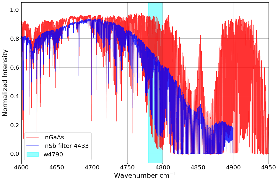
Figure C1 Sample solar spectra for InGaAs (in red) and InSb using the filter 4433 (in blue). Both spectra were collected in Ny-Ålesund.

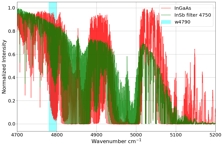
Figure C2 Sample solar spectra for InGaAs (in red) and InSb using the filter 4750 (in green). Spectra were collected in Ny-Ålesund and Bremen.

Figure C3 The transmission curve for the filter 4433 and a zoom-in for the w4790 window.

Figure C4 The transmission curve for the filter 4750 and a zoom-in for the w4790 window.

Appendix D: Reduced-resolution tests

In this section we show the results of the resolution tests performed on 3 clear days in Bremen using the 4750 cm⁻¹ filter: 2 March 2021 for the first test shown in Fig. D1 and 26 and 28 April 2021 for the test shown in Fig. D2. On the first day, four different resolutions where measured. These included the controls: TCCON (reference) with an optical path difference (OPD) of 68.3 cm (in black) and the original NDACC OPD of 180 cm (in red). Then there were tests at 90.01, 64.3, and 45.01 cm (in blue). On the second and third day, lower resolutions were measured: 18.01, 12.01, 9.01, 6.01, 4.51, 3.01, 2.26, and 1.81 cm (in green) with the corresponding controls, NDACC and TCCON.

The strategy on the first day consisted of 15 min of measurements of each resolution and two alternating measurements of TCCON (in red) every 30 min as a control. In total, four rounds of measurements were performed. The figure below shows the mean (black dot), the measurements (smaller color dots), and the variation of each set of measurements.

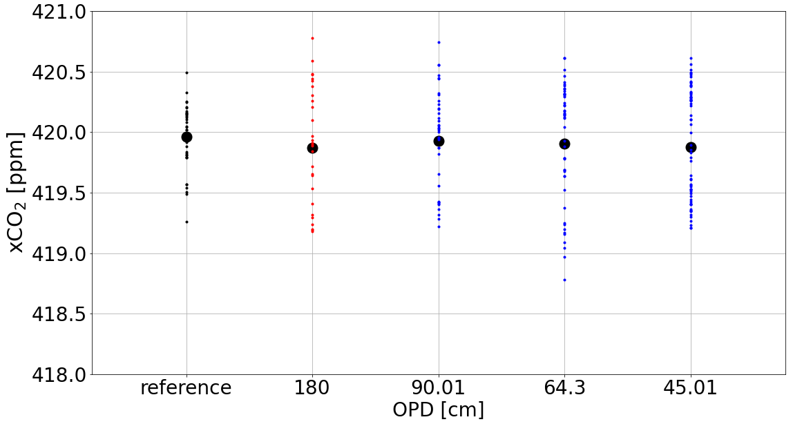
Figure D1 The variation in xCO₂ of the resolution test by OPD for the higher resolutions tested. In black is the reference spectrum: xCO₂ retrieved from 6300 with the standard TCCON resolution of 45 cm. In red is the standard NDACC resolution of 180 cm, and in blue are the test resolutions for InSb spectra of 90, 63, and 45 cm.

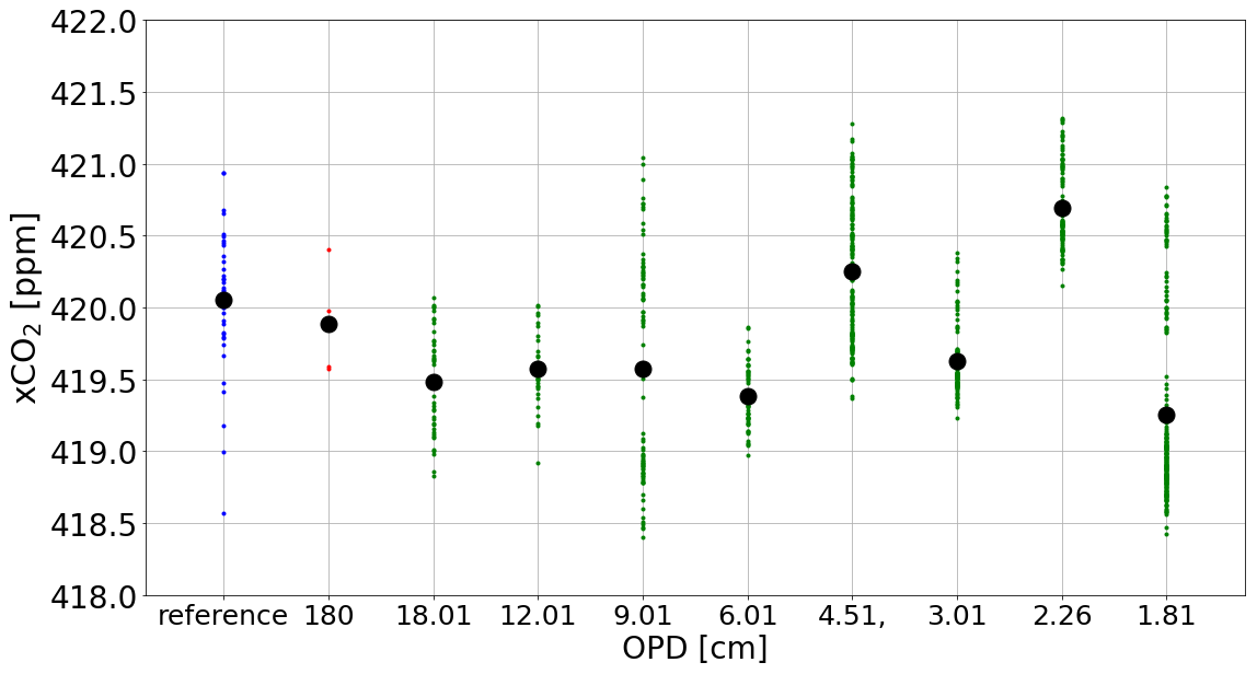
Figure D2 The variation in xCO₂ in the resolution test by OPD for the lower resolutions tested. In blue is the reference spectrum: xCO₂ retrieved from 6300 with the standard TCCON resolution of 45 cm. In red is the standard NDACC resolution of 180. In green are the resolution tests for InSb spectra.

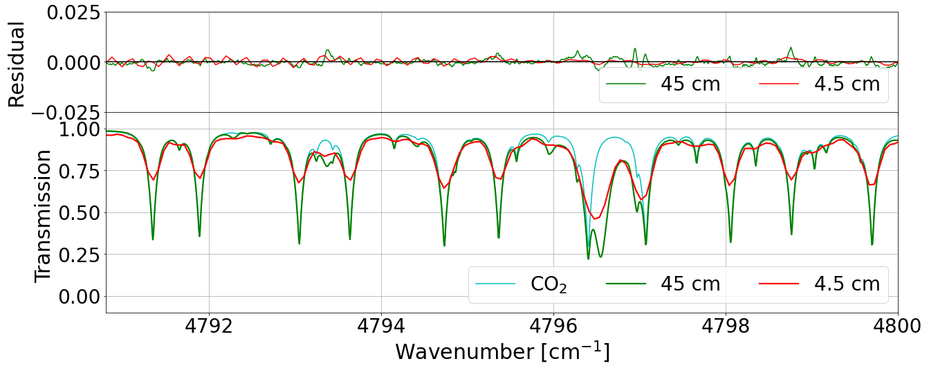
Figure D3 Spectral fit and residuum of spectra of different resolutions. In green are the calculated spectra (Tm) with OPD 45 cm, and in red are the calculated spectra (Tm) with OPD 4.5 cm; in cyan are the CO₂ absorption lines.

The lower-resolution tests were performed (and results are shown in Fig. D2) with more random alternations but covered at least 15 min of measurements. The control TCCON measurements are performed at the beginning, in the middle, and at the end of the other measurements.

In Fig. D1 in the 64 cm OPD there are a few outliers. This is seen below the 419 ppm line for resolution 64.3 that has the lowest values among the rest of the tests.

The goal is to find the optimal resolution to improve the precision of the retrieval without compromising other aspects. An OPD lower than 45 cm does not significantly decrease the standard deviation of the mean from the increased number of measurements; therefore, we see no advantage in using lower resolutions. At the same time, 45 cm results in a well-resolved spectral fit, while a lower resolution starts to misrepresent the actual spectral lines.

Appendix E: Temperature dependence and alternative retrieval

As mentioned in Sect. 2.2 the band chosen is a “hot” band, which makes the retrieval temperature-dependent. With a lower mean energy level of $E^{\prime \prime }=\mathrm{858}$ cm⁻¹ the estimated theoretical error for a 2 K error in temperature is between 1.2 % and 1.8 % of the retrieved xCO₂.

One alternative window considered for this retrieval was the third isotope ¹⁶O¹²C¹⁸O (named 3CO₂ by HITRAN) in the same region as shown in Fig. E1 in yellow. Using the 3CO₂ band would yield a less temperature-dependent product because it has a lower mean energy level, $E^{\prime \prime }=\mathrm{217}$ cm⁻¹.

However, tests showed that due to the averaging kernels' low sensitivity towards the surface, the retrieval does not capture the seasonal cycle properly and is heavily dependent on the a priori. This alternative brings benefits as it captures the stratosphere; however, there is an offset to be calculated that is possibly due to GFIT's assumed isotopic fractionation, which can be easily corrected for.

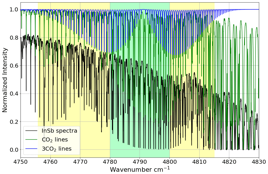
Figure E1 Spectra and spectral lines: in black is a sample InSb spectrum, in green are FTIR atlas CO₂ lines, and in blue is CO₂. Two windows are shown: in green is the original w4790, and in yellow is the alternative window to use 3CO₂.

Appendix F: Pressure dependence and the pressure sensor

The pressure sensor used in Ny-Ålesund is the Digiquartz 6000-16B barometer with an accuracy of ±0.08 hPa. This sensor is not recalibrated regularly. Single comparisons to other sensors have been performed, and the difference was within the error of both instruments. The pressure sensor used in Burgos is the Setra 270-12V with a range 800–1100 hPa and an accuracy (at constant temperature) of ±0.05 % FS. This sensor has been compared twice since 2017. Once in September 2017, against Japan's CS106, the difference was within the sum of the precisions, so no calibration was needed. In November 2023 the differences against PTB330 from Japan were again within the sum of the precisions, but 0.041 hPa was added to the Setra 270 as an offset.

We suggest calibrating the sensor biannually or more frequently to avoid drifts. Drifts in the pressure measurements could introduce a retrieval error; this would affect the xCO₂ retrieved from w4790, while it would not affect the xCO₂ retrieved from TCCON because the pressure cancels out due to the use of O₂.

Appendix G: The line list in w4790

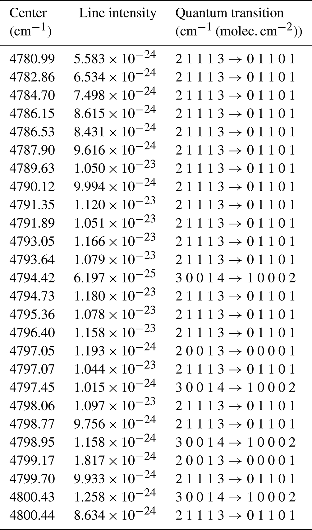
Table G1 The mid-IR line list used in this study. Each line is characterized by the center wavenumber. Additionally, the corresponding molecular transition for the quantum numbers ν₁, ν₂, l₂, ν₃ and n is given. Three of these, ν₁, ν₂, and ν₃, express the number of quanta activated for each fundamental; l₂ is the l value for the degenerate ν₂ fundamental and its overtones. The fifth integer is the nth component of the Fermi interacting ν₁ and 2ν₂ vibrational states including their overtone and combination states (Toth et al., 2008). Data are taken from the TCCON GGG2020 line list, adapted from HITRAN (Rothman et al., 2009).

Appendix H: TCCON's lCO₂ window

TCCON is working on a new window in the same region centered at 4852.87 cm⁻¹ of 86.26 cm⁻¹ width that uses the same band to retrieve CO₂. The lCO₂ window was not developed for the same purposes that w4790 was developed; therefore, it is not ideal for retrieving historical NDACC spectra from Ny-Ålesund as done in this paper because the window is located past the 50 % cut-off of the 4433 filter used there. However, the window would work with TCCON and NDACC spectra with other filters such as 4750 shown in Appendix C.

The lCO₂ and the w4970 windows have a large difference in the averaging kernels. The lCO₂ AKs have little variation with SZA. For low SZA w4790 is closest to 1 and shows the largest difference between the two windows.

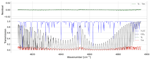
Figure H1 An example of the calculated spectra (Tc) and the measured spectra (Tm) for the lCO₂ window, CO₂ absorption lines, other gases, and the residual (Tm − Tc) for typical spectra recorded in Ny-Ålesund.​​​​​​​

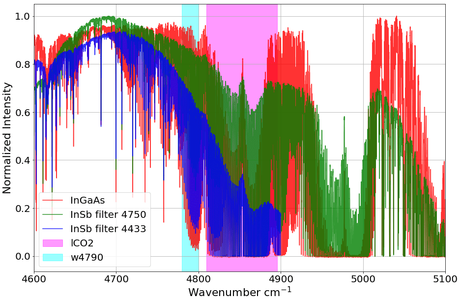
Figure H2 Sample solar spectra for InGaAs (in red) and InSb using the filter 443 (in blue) and filter 4750 (in green), collected in Ny-Ålesund. The lCO₂ window is in magenta.

Figure H3 The w4790 averaging kernels averaged to 1^∘ for InGaAs in Ny-Ålesund.

Figure H4 The lCO₂ averaging kernels not averaged for InGaAs in Ny-Ålesund.

Appendix I: Supplemental plots

Figure I1 The w4790 averaging kernels averaged to 1^∘ for InSb Ny-Ålesund spectra.

Figure I2 The averaging kernels for the Burgos TCCON product (from GGG2014).

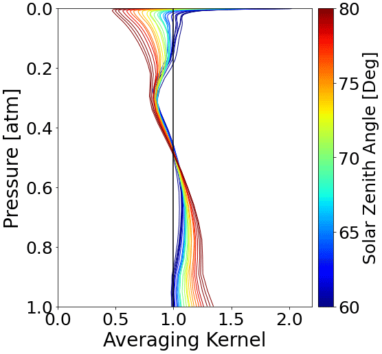
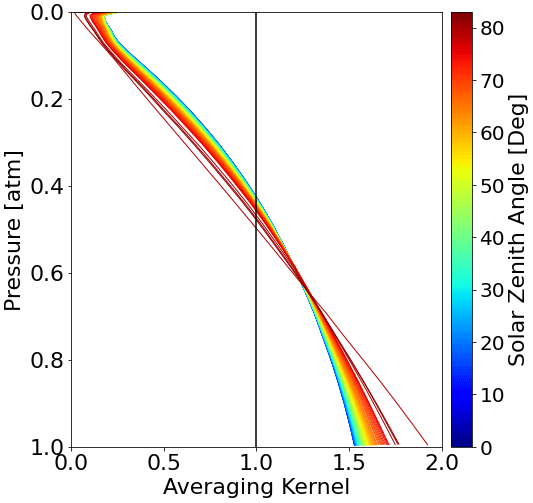
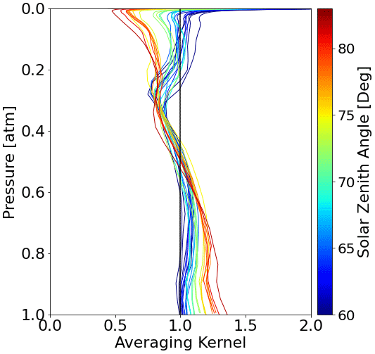
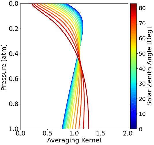
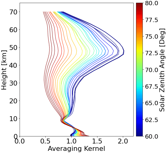
Figure I3 The w4790 averaging kernels averaged to 1^∘ SZA for InGaAs Ny-Ålesund spectra plotted against altitude in kilometers.

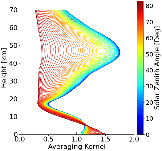
Figure I4 The w4790 averaging kernels averaged to 1^∘ SZA for InGaAs Burgos spectra plotted against altitude in kilometers.

Figure I5 The standard (b) and deseasonalized or modified (a) a priori profiles for Burgos.

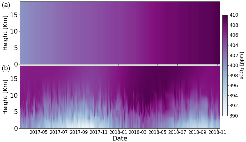
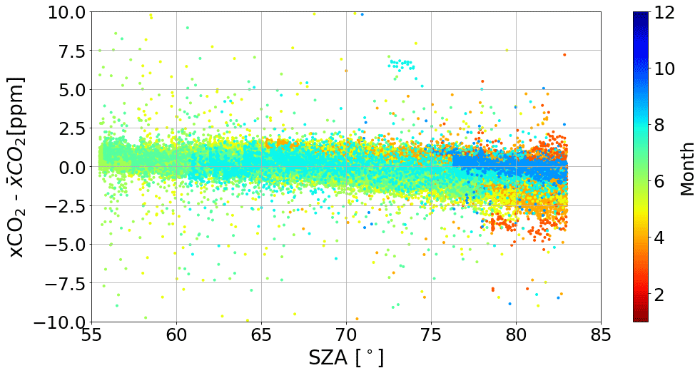
Figure I6 Ny-Ålesund 6300 xCO₂, prior to the air mass correction, minus the daily mean of the corresponding month.

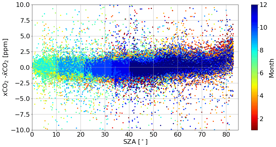
Figure I7 Burgos 6300 xCO₂, prior to the air mass correction, minus the daily mean of the corresponding month.

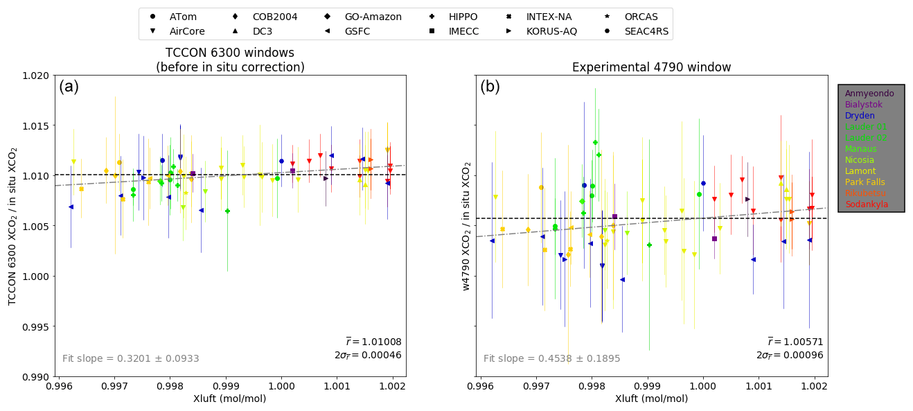
Figure I8 (a) Ratio of TCCON xCO₂ to in situ xCO₂ against xluft between 0.996 and 1.002. (b) Ratio of w4790 xCO₂ window to in situ xCO₂ against xluft between 0.996 and 1.002.

Figure I9 Histogram of the standard deviation of the daily means of CO₂ in Ny-Ålesund.

Figure I10 Histogram of the standard deviation of the daily means of CO₂ in Burgos.