the Creative Commons Attribution 4.0 License.
the Creative Commons Attribution 4.0 License.
 | 11 Oct 2023
Revision of an open-split-based dual-inlet system for elemental and isotope ratio mass spectrometers with a focus on clumped-isotope measurements
Stephan Räss
Peter Nyfeler
Paul Wheeler
Will Price
Markus Christian Leuenberger
In this work, we present a revision of an open-split-based dual-inlet system for elemental and isotope ratio mass spectrometers (IRMSs), which was developed by the division of Climate and Environmental Physics of the University of Bern 2 decades ago. Besides discussing the corresponding improvements we show that with this inlet system (NIS-II, New Inlet System II) external precisions can be achieved that are high enough to perform measurements of multiply substituted isotopologues (clumped isotopes) on pure gases. For clumped-isotope ratios and of oxygen, we achieved standard deviations of and , respectively, that we calculated from 60 interval means (20 s integration) of pure-oxygen gas measurements.
Moreover, we report various performance tests and show that delta values of various air components can be measured with precisions of the order of tens of per meg and higher with the NIS-II. In addition, we demonstrate that our new open-split-based dual-inlet system allows us to measure some of these delta values with significantly higher precisions than an NIS-I (precursor of the NIS-II) and conventional changeover-valve-based dual-inlet systems (tests performed with two dual-inlet systems built by Elementar and Thermo Finnigan). Especially, our measurements point out that our inlet system provides reliable results at short idle times (20 s) and that the corresponding data do not need to be corrected for non-linearity. However, the sample consumption of our open-split-based dual-inlet system is several orders of magnitude higher than that of changeover-valve-based ones (0.33 sccm versus 0.005 sccm; standard cubic centimetres per minute).
Due to the successful preliminary tests regarding measurements of clumped-isotope ratios, we will continue our work in this area to perform clumped-isotope studies according to common practices.
- Article
(2644 KB) - Full-text XML
- BibTeX
- EndNote


Among the established peripherals for sample introduction to isotope mass spectrometers (IRMSs), there are changeover-valve-based dual-inlet systems. While the external precision of such inlet systems is of the order of hundredths of per mil (Leuenberger et al., 2000) and thus high enough for many common applications, it is too low for measurements requiring a very high precision; for example, the annual variability in measured in ambient air is of the order of tens of per meg (Berhanu et al., 2019). To make measurements like these possible, more than 20 years ago, the division of Climate and Environmental Physics of the University of Bern developed an open-split-based dual-inlet system whose basic principle was adapted from gas chromatography–mass spectrometry (GC–MS) open splits (Brand, 1995).
Basically, changeover-valve-based dual-inlet systems consist of two individual metal bellows (one for storing the sample gas and the other for the standard gas), two separate gas lines and a changeover valve block. The metal bellows, which typically have a volume of between 20 and 100 mL (Leuenberger et al., 2000), are compressible such that the signals of the two gases can be equalised. During operation, the gases are transported from the two bellows to the changeover valve block; there, the gas is selected that is admitted to the mass spectrometer. By switching between the two gases the isotope ratios and the corresponding delta values can be determined. To guarantee a similar gas consumption for both sides of the inlet system, the gas that is not admitted to the mass spectrometer is consumed by one of the inlet system's pumps.
Unfortunately, these changeover-valve-based dual-inlet systems have some drawbacks that deteriorate the measurement precision; firstly, as the gas flux through such inlet systems is not continuous and many metallic surfaces are present, surface adsorption/desorption effects on these surfaces may occur (Leuenberger et al., 2015). This can in turn lead to variations in the gas composition. Secondly, isotope fractionation (Leuenberger et al., 2000) may occur because the pressure of the gases under study is altered through the inlet system's valves.
As reported by Leuenberger et al. (2000), these issues can be overcome using an open-split-based dual-inlet system. The primary goals of Leuenberger et al. (2000) were to improve the pressure and temperature adjustment, to reduce adsorption/desorption effects on metallic surfaces and to build an inlet system that is as symmetrical as possible. To reduce signal variations to 0.25 ‰, the pressure and the temperature may not vary more than 0.1 mbar and 0.03 ∘C, respectively (Leuenberger et al., 2000). Due to these requirements, the gas flow rates of the measured gases must be highly constant; otherwise, non-linearity effects may lead to fractionations noticeable at the scale of per meg (Leuenberger et al., 2000). The three aims were achieved as follows (Leuenberger et al., 2000): the changeover valve block was replaced by a Y-shaped open-split interface, which was situated inside an aluminium container. The temperature of the container could be regulated utilising cartridge heaters, and, for the pressure regulation, a vacuum pump and a pressure controller were used. Through this design, it was possible to fully separate the inlet system from the ion source. For the transfer of gas from the gas containers to the open split and from the open split to the mass spectrometer glass capillaries were used.
The dual-inlet system we present in this paper, the “New Inlet System II” (NIS-II), is the successor of the first version (NIS-I) described in the paper by Leuenberger et al. (2000). In addition to high-precision measurements of conventional elemental and isotope ratios, the NIS-II was built to detect multiply substituted isotopologues (clumped isotopes). For clumped-isotope studies, the corresponding isotope ratios usually need to be measured with precisions of the order of 10−5 to 10−6 (Eiler, 2007).
In general, the basic working and design principles of both versions of the NIS are identical. However, the NIS-I had the following two major disadvantages that we have now eliminated.
-
Since the open-split interface was implemented through a Y-shaped piece of glass (two inlets for the transport of standard or sample gas into the open split and one for the gas transfer to the IRMS), it was difficult to purge the open split thoroughly. To attain good results, the glass capillaries had to be equipped with rubber seals at their ends and had to be positioned very precisely. Not only did the proper positioning of the rubber seals require many attempts, but also position checks were necessary regularly.
-
The second drawback concerns the mechanism responsible for switching between the sample (SA) and the standard (STD) gas. This mechanism was based on two pneumatic pistons, which were put in motion through two electromagnetic valves. Although this mechanism did not have a noticeable influence on the measurement results, it was not ideal; to ensure a gas tightness over 5 decades of pressure, the pneumatic valves had to be equipped with two-step seals that required frequent maintenance.
In what follows, we first describe the design and working principles of the NIS-II. Thereafter we report the results of different studies we carried out to assess the performance of the new inlet system. Moreover, we present a comparison of our new inlet system to its precursor as well as to a common changeover-valve-based dual-inlet system (Elementar iso DUAL INLET). The central part of the paper, the feasibility study of clumped-isotope measurements of air components, is documented at the end.
2.1 Design principle
The housing of our new dual-inlet system, the NIS-II, consists of a cylindrical aluminium frame with an inner diameter of 31 cm and a wall thickness of 2 cm. The housing, whose height is 11 cm, can be closed with a cap made of acrylic glass having a thickness of 2 cm. This cap can in turn be fixed to the aluminium frame using 16 screws. Next to the corresponding screw holes there is a circular recess for a rubber seal that improves the gas tightness of the container (see Fig. 1).
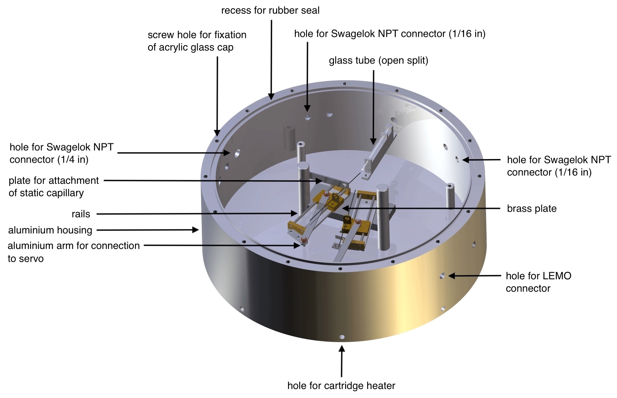
Figure 1Computer-aided design (CAD) image of the NIS-II container created by the mechanical workshop team of the division of Climate and Environmental Physics of the University of Bern with annotations added by the authors.
In the centre of the container, we installed an aluminium base plate on which different components are mounted: on the top end of the base plate there is a glass tube acting as an open-split interface. This tube is closed at its back end and has a length of approximately 4 cm. This glass tube, which has an inner diameter of 1.4 mm, is fixed to the base plate using an intermediate piece of aluminium, which allows for inserting the open split in a horizontal position. While the intermediate piece of aluminium is screwed down on the base plate, the glass tube can be removed easily as the fixation to the intermediate piece is realised through tape. On the lower end of the container's base plate, there are two Blue Bird Standard BMS-660 servos, which together constitute the centrepiece of the dual-inlet system's switching mechanism. These servos can be controlled through an Olimex PIC-P18 development board (outside of the container) and the mass spectrometer's software (Elementar isoprime precisION running IonOS). In contrast to the pneumatic valves of the NIS-I, the servos require little maintenance and do not influence the temperature inside the container significantly. Each of the servos' arms is in turn attached to a brass plate that can be moved along 8 cm long rails. On each of these moveable brass plates, we installed a in. Swagelok bulkhead union that is used for the fixation of a gas transfer capillary. To fix the capillary, we first remove the union's nuts, guide the capillary through the union and add a BGB Analytik graphite–Vespel in. × 0.4 mm ferrule; then we mount the nuts again.
As pointed out before, the gas transfer is realised through glass capillaries. For this transfer at least three capillaries are required: one capillary is static and connects the open split to the IRMS. The other two capillaries, which are fixed to the moveable brass plates, transfer gas from the containers for the sample and standard gas, respectively, to the open split. Please note that the static capillary is installed in a fashion similar to the other two, except that the capillary holder is not mounted on a moveable brass plate instead but on a static piece of aluminium near the centre of the base plate.
For guiding the capillaries into the container, we integrated five Swagelok NPT (national pipe thread) connectors ( in.) into the container walls. Of these five connectors at least three are used, namely one per capillary. For the fixation of the capillaries, the same principle was applied that was used for the capillary holders mounted on the moveable brass plates.
In addition to these five connectors, we added three larger Swagelok NPT ports ( in.). One of these ports is used for connecting an ANALYT-MTC pressure controller to the inlet system that, along with a KNF N 920 (KT.29.18G) feed pump, stabilises the pressure inside of the container. For most applications, the pressure inside of the container is set to a value between 20 and 250 mbar; in fact, this eventually depends on the capillaries and the desired signal height. The second of these three ports is connected to a pure-argon gas cylinder, which is used for the purging of the container; typically, the flow rate of this gas is held constant at a value between 5 and 10 mL min−1. Between the container and the pressure controller as well as between the container and the gas cylinder there are Nupro gas shut-off valves, which can be used to isolate the container from the laboratory. In addition to the gas ports, we embedded three LEMO connectors in the container walls which are used for the signal transmission and the power supply of the electronic components situated on the inside of the container.
To regulate and stabilise the temperature of the NIS-II container, we use electric cartridge heaters. For the placement of these heaters, we drilled eight equally distributed holes into the bottom end of the container walls. Moreover, for the fixation of the heaters with screws, eight holes were drilled into the bottom of the container. To improve the heat transmission, we dipped the cartridge heaters into a heat sink compound before introducing them into the holes. The heating status of the container can be monitored utilising an external temperature control unit, which responds to a Pt100 temperature sensor located on the inside of the NIS-II container below the aluminium base plate. To reduce the occurrence of thermal fractionation the set temperature should be similar to the temperature of the mass spectrometer.
2.2 Working principle
The NIS-II is built in such a way that there is an uninterrupted gas flow through all of the capillaries. During operation, one of the two moveable capillaries is situated inside of the open split, while the other is kept outside; while the gas of the former capillary is automatically transferred to the static capillary, which is also situated inside of the open split, the gas of the other capillary is poured into the free space of the NIS-II container. As the static capillary is connected to the mass spectrometer, the gas eventually reaches the ion source. During this procedure, the NIS-II container is constantly flushed with a purge gas and is held at a constant pressure.
When switching between the moveable capillaries, the system goes through the following steps: at the end of each measuring interval the capillary that is currently outside of the open split is inserted into it, and, subsequently, the other one is retracted. By fully inserting the former capillary into the glass tube before the latter is pulled out, we ensure that the open split remains sealed off from the container atmosphere. However, as this type of sealing also relies on a gas flow rate that is high enough to prevent container gas from entering the open split, we had to find a way to detect possible leaks. This can for example be achieved by selecting a container purge gas that the mass spectrometer's Faraday collector array can detect. For the studies presented in this work, we used pure argon (stored in a regular steel cylinder).
The fundamental principle that is applied to transfer gas from the two gas sources to the mass spectrometer is the generation of flow through a pressure gradient. To provide a continuous gas flow, the pressure has to gradually decrease from the gas sources to the mass spectrometer.
The gas flow rate through a capillary, which depends on the pressure gradient as well as on the length and the inner diameter of the capillary, can be estimated using the Hagen–Poiseuille equation:
In Eq. (1), denotes the volumetric flow rate; η is the dynamic viscosity of the fluid; r and l are the inner radius and the length of the capillary, respectively; and Δp is the pressure difference between the two ends of the capillary.
Eventually, the length and the radius of any capillary are selected based on the required flow rate. While the flow rates of the capillaries of the switching mechanism (gas cylinders to the NIS-II) have a lower limit, namely the minimal purge flow rate (see Sect. 3.2), the flow rate of the static capillary (NIS-II to IRMS) is restricted by the range of detectable signals; for our Elementar isoprime precisION the range is 0 to 100 V. For instance, if the pressure of the NIS-II is set to 20 mbar and an air sample is transferred to the IRMS via a capillary with a length of 1.7 m and an inner diameter of 100 µm, the flow rate is approximately sccm (standard cubic centimetres per minute); at a trap current of 200 µm, the signal on the u e−1 cup turns out to be around 50 V (or A).
While changeover-valve-based dual-inlet systems need to adjust the gas pressure to compensate for the gas loss, namely through bellow compression, this is not necessary for our system; throughout the entire gas transfer from the gas sources via the NIS-II to the mass spectrometer the gases are subjected to the same pressure conditions. If one would like to alter the pressure inside of the system, this can be achieved with the help of the ANALYT-MTC pressure controller and the KNF N 920 feed pump. This pressure regulation in turn allows for altering the gas flow into the ion source and therefore the signal intensity.
For the studies presented in this section, we measured gas cylinders containing either compressed air or pure oxygen from Carbagas, Switzerland. In the following, when referring to gas cylinders we will use the prefix “LUX” for aluminium Luxfer cylinders and “SC” for regular steel cylinders. Typically, for the air measurements we used gas from cylinders LUX 3588 and LUX 3591. For oxygen measurements cylinders SC 84567 (O2≥99.998 %), SC 62349 (O2≥99.9995 %) and SC 540546 (O2≥99.9995 %) were available.
Our main measurement setup, which was set up according to the descriptions in Sect. 2, consists of the Elementar isoprime precisION IRMS and the open-split-based NIS-II. For comparison purposes, we also used the changeover-valve-based Elementar iso DUAL INLET for certain experiments. The two bellows of the iso DUAL INLET have volumes of around 100 and 40 mL, respectively; the stainless-steel capillaries have a length of 635 mm and an inner diameter of 0.004 in. The crimps are set in such a way that a depletion of the major beam of approximately 12 % to 15 % over a 12-comparison acquisition is achieved; with new non-crimped capillaries, the depletion rate is normally above 50 %.
Our isoprime precisION is equipped with a Faraday collector array for measuring air components. This array consists of 10 cups designed for measuring the mass-to-charge () ratios 28 to 30, 32 to 36 u e−1, and 40 and 44 u e−1. Hereafter, we will drop the units of mass-to-charge ratios for the sake of simplicity. The delta values we present in this section were calculated from the measurement signals as described in Appendix A. The notation we adopted for delta values referring to isotope ratio R is δR.
The measurements we carried out with the Elementar isoprime precisION were composed of six measuring intervals for sample gas and six or seven measuring intervals for standard gas; these intervals were executed in alternating order. In the following, measurements of this type will be denoted as “SA–STD measurements”. The integration time of each of the measuring intervals was set to 20 s. Unless otherwise stated, external precisions derived from such a measurement series were always assessed by calculating the standard deviation of the mean delta values (or isotope ratios) of the individual measurements. For the assessment of the internal precision of delta values (or isotope ratios), we computed the mean value of the standard errors in the individual measurements.
The first performance test we carried out concerned the purging of the new open split. Thereafter, we studied the measurement precision limits and the signal stability of the new measurement setup. As a next step, we determined the precisions with which delta values of air components can be measured and compared these results to those obtained with the NIS-I and the iso DUAL INLET. As a last step, we used the NIS-II to measure air and pure oxygen to assess the feasibility of clumped-isotope measurements with our setup.
In the following subsections, we first report our experience with the new inlet system's maintenance and then discuss the previously mentioned studies along with their results.
3.1 Maintenance
Concerning the maintenance of the NIS-II, we saw an improvement when compared to the first version of the inlet system; within 1 year of almost daily use, the only maintenance required was the removal of dust from the rails of the capillary switching mechanism. This dust, which mainly accumulates due to mechanical abrasion, had to be removed twice in this period. After cleaning the rails with alcohol, they have to be greased with an oil having a low vapour pressure. When including the time needed to open and close the NIS-II container, this procedure takes approximately 30 min. When the NIS-II is operated over longer periods, at some point, the servos driving the capillary switching mechanism have to be replaced. This is usually the case after 1 to 2 years. Nevertheless, when the NIS-II is heavily used or the servos are of poor quality, this replacement might also be due sooner.
3.2 Open-split purging
As the open-split interface is not mechanically sealed off from the dual-inlet system's container atmosphere, this has to be ensured by establishing a gas flow rate that is high enough to prevent container gas from reaching the ion source. In the following, this gas flow rate will be referred to as “purge flow rate”. This flow rate must not be confused with the flow rate of the container purging gas (argon).
To study the influence of the purge flow rate on the measurement signals, we connected the pure-oxygen gas cylinder SC 84567 to the standard inlet of the NIS-II and performed 12 time scans (Faraday cup signal recording at a fixed acceleration voltage) at different volumetric purge flow rates. To vary this flow rate, we introduced an ANALYT-MTC mass flow controller (MFC) of the 358 series between the gas cylinder and the NIS-II. As the pressure inside of the NIS-II container was kept constant, namely at 20±1 mbar, the pressure variation through the MFC allowed for altering the volumetric purge flow rate.
In Fig. 2, the mean signal of the cup recorded during the aforementioned time scans is shown as a function of the measured volumetric flow rate, namely in cubic centimetres per minute (measured) as well as in standard cubic centimetres per minute (calculated). We performed the standardisation with respect to pressure (101 325 Pa) and temperature (273.15 K). For the calculations, we used the ideal gas law as well as the temperature and the pressure readings of the MFC. As an aside, it may be mentioned that the relevant pressure is not the pressure reading of the MFC but the mean value of the pressure reading and the NIS-II container pressure (20 mbar); the reason for this is that according to Eq. (1) the pressure between the MFC and the NIS-II container decreases linearly.
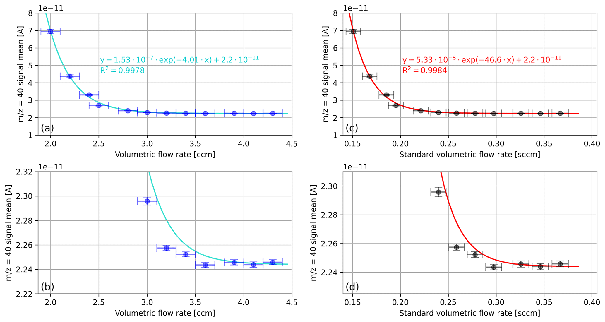
Figure 2Mean cup signals recorded during a series of 3 min oxygen time scans corresponding to different volumetric flow rates. (a) Signals of the cup as a function of the measured volumetric flow rate in cubic centimetres per minute. (c) Same data as in panel (a) but in standard cubic centimetres per minute (mass flow). (b) Zoomed-in view of panel (a); (d) zoomed-in view of panel (c). The vertical error bars correspond to the standard deviations of the signal. In panel (a), the horizontal error bars indicate the approximate fluctuation in the flow rate reading (0.1 sccm), and in panel (b) this error was converted to standard cubic centimetres per minute.
The data shown in Fig. 2 indicate potential contaminations of pure oxygen with the gas of the NIS-II container atmosphere. This gas is mainly composed of the purge gas argon and the analyte. Additionally, as the LEMO connectors of the container are only gas-tight to a certain degree, at pressures distinctly below atmospheric pressure, it cannot be excluded that also small amounts of laboratory air are present in the container atmosphere.
As can be seen from Fig. 2, the signal decreases exponentially and levels out around 3.9±0.1 ccm (cubic centimetres per minute), which corresponds to 0.33±0.01 sccm. Because the NIS-II container was primarily filled with argon, it can be concluded that for purge flow rates exceeding 0.33 sccm the open split is isolated from the container atmosphere to a satisfactory degree. Concerning sample consumption, this implies that a measurement consisting of 12 measurement intervals with an integration time of 20 s and an idle time of 60 s requires a total gas volume of around 5.28 scc (standard cubic centimetre) (16 min ⋅ 0.33 sccm). If the idle time of the measurement is reduced to 20 s, only half the amount of gas is needed.
When comparing the new open split to the Y-shaped open split of the NIS-I, it is noticeable that the minimum purge flow rate of the new open split is higher by a factor of 2; for the NIS-I, 0.16 sccm (120 nmol s−1) was required (Leuenberger et al., 2000). Furthermore, the sample consumption of our open-split-based dual-inlet systems is higher than that of a changeover-valve-based dual-inlet system, namely due to the purging of the open split; the sample consumption of conventional dual-inlet systems is around 0.005 sccm (estimated from measurements with a Thermo Finnigan DELTAplus XP and its integrated dual-inlet system). The gas consumption of our system mainly depends on the design of the open split.
Although the minimum purge flow rate of the straight open split is higher than that of its Y-shaped precursor, we consider it a major improvement; during operation, the new open split causes no noteworthy problems. Apart from that, it is easy to install, replace and manufacture.
As stated previously, the length and the inner diameter of any capillary are selected based on the flow rate. To connect the gas cylinders to the NIS-II, we normally use two capillaries that are connected by a press fit; the capillary ending in the cylinder usually has a length of around 1.5 m and an inner diameter of 180 µm, whereas the capillary ending in the NIS-II typically has a length of around 1 m and an inner diameter of 100 µm.
3.3 Measurement precision limits
The measurement precision that can be attained with an IRMS and its inlet system is limited by different factors. In this subsection, we discuss the system noise and the errors associated with counting statistics because those are closely linked with the measurement setup itself. Nonetheless, it is important to be aware of the fact that external factors such as sample purity and sample handling that have an influence on the measurement precision also exist.
3.3.1 System noise
To assess the system noise of the Elementar isoprime precisION, we took the following approaches.
-
We closed the mass spectrometer's main gas admission valve, evacuated the mass spectrometer and then recorded the Faraday collector signals for 5 min. In the following, we will refer to these measurement signals as “collector zeros”.
-
We turned off the acceleration voltage (AV) and then recorded the cup signals for 5 min while admitting air to the mass spectrometer through the NIS-II. We will refer to the corresponding data as “electronic noise”.
In Table 1, the outcomes of the measurements outlined before are shown. In addition, to get a first impression of the measurement precision of regular measurements, we also performed a 5 min time scan of compressed air at an acceleration voltage of around 4461 V. The results of this measurement, which were derived from the raw data (no background corrections), are also shown in Table 1.
Table 1Faraday cup signal means determined with an Elementar isoprime precisION in the absence of gas (collector zeros) as well as in the presence of air (LUX 3588 admitted with the NIS-II). For the electronic zeros, the acceleration voltage was turned off. The mean values were calculated from each of the 5 min measurements without removing any data points and without applying any corrections. For the uncertainties in the cup signals the standard deviations of the cup signals were computed. In the first column of the table, the mass-to-charge ratios of the 10 Faraday cups are indicated.
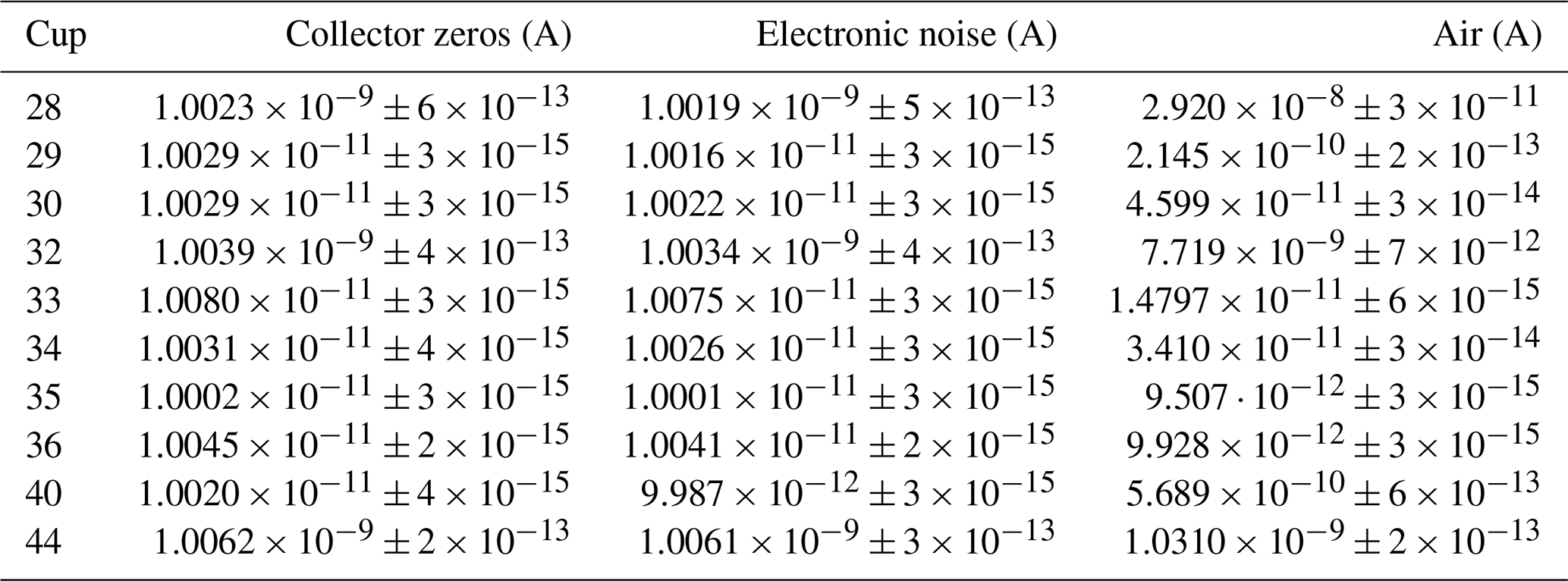
When comparing the collector zeros to the electronic noise shown in Table 1, it can be seen that they are almost identical. This is reasonable because in neither case are ions reaching the cups; thus, signals are generated by system noise alone. Furthermore, it stands out that the mean values of these noise indicators and the corresponding standard deviations are very similar for all of the cups, except for the dominant mass-to-charge ratios 28, 32 and 44; these are measured at low gain (109 Ω resistors) instead of high gain (1011 Ω resistors). The means and standard deviations of these three cup signals are around 2 orders of magnitude higher than the corresponding values of the remaining cups. Furthermore, from the standard deviations of the collector zeros and the electronic noise one learns that the cup signals with high and low gain can be recorded with maximum precisions of the order of and A, respectively.
When comparing the collector zero measurement to the measurement of air, it is noticeable that the standard deviations are very similar for mass-to-charge ratios 33, 35, 36 and 44. In contrast, the standard deviations of the other cup signals are around 1 to 2 orders of magnitude higher for the air measurement; for instance, this can be caused by recombination and scrambling in the ion source or by statistical effects. Although we cannot rule out that the discrepancies were induced by the inlet system, this is rather unlikely since a deterioration of the standard deviation cannot be observed for all of the cup signals.
3.3.2 Counting statistics
As mentioned in the introduction of this subsection, among the limits of the system's measurement precision there is the so-called “shot noise limit”, which is associated with counting statistics. Basically, this type of noise occurs because the number of ions generated by electron impact ionisation is not constant but approximately distributed according to the Poisson distribution. When denoting the number of ions as N, the standard deviation (or absolute error) of the Poisson distribution is given by and the relative error is given by .
In Fig. 3a, shot noise limits (relative error in the Poisson distribution) and relative standard errors in Faraday cup signals are displayed. For the calculation of these values we used the first 60 s of the time scan of air summarised in Table 1; additionally, we computed the same standard errors for the collector zero data set of this table (in Fig. 3 denoted as “background”). From Fig. 3a it can be seen that the standard errors in the background are very close to the shot noise limit; this also holds for some of the signals recorded during the time scan of air, namely for , , and . Nevertheless, for the time scan of air, most of the standard errors are higher than the errors in the other two data sets. From this, it can be concluded that, in general, effects other than counting statistics are limiting the measurement precision. This becomes even clearer when the same error calculations are performed for the isotope ratios (Fig. 3b). In addition, we repeated the error calculations for the complete data sets (300 s) and came to the same conclusions.
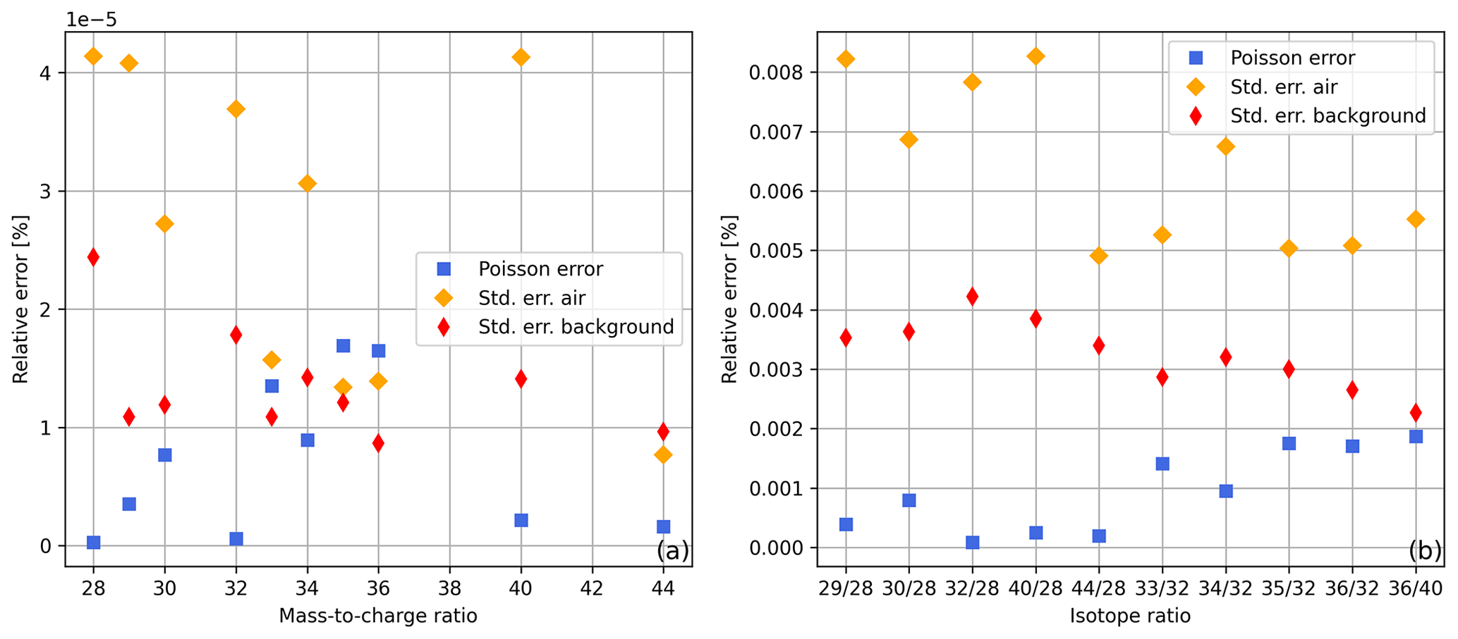
Figure 3Relative Poisson and standard errors in (a) ion beams and (b) isotope ratios calculated from the first 60 s of the uncorrected time scans summarised in Table 1 (collector zero data for background error and air data for remaining errors). For the standard errors in the ion beams the standard deviations were divided by ; this corresponds to the square root of the number of 0.1 s signal means we used. The relative errors in isotope ratios were calculated by adding up the relative errors in ion beams S1 and S2.
3.3.3 Signal stability
To study the signal stability affected by noise processes, we performed 1 h time scans of air (LUX 3588) and used the Allan variance σ2 (Allan, 1966). This variance, which is calculated from N samples of the quantity ϕ, is given by
In this equation, τ denotes the sample time and T is the period of sampling. To analyse the signal stability of different isotope ratios of air components, we considered the case of τ=T (no dead time). For and we used the signal averages starting at times nT and nT+τ, respectively; these were calculated for averaging times τ∈ of [1 s, 650 s]. In Fig. 4, we present the Allan variance of isotope ratio as a function of the averaging time. From this figure one can see that the variance reaches its minimum at around 81±6 s. This means that the measurement precision can be increased by signal averaging but only up to this value. To get rid of the largest fluctuations, the minimum of the Allan variance was not determined from the raw data but from a centred moving average (±10 s) of the original data set. The uncertainty in this minimum was in turn assessed by computing the standard deviation of the instants of time that were used for the calculation of the corresponding element of the moving average.
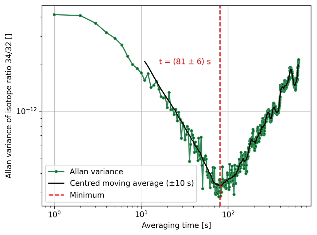
Figure 4Allan variance of isotope ratio as a function of the averaging time (1 s steps). The corresponding data were recorded during a 1 h time scan of air (LUX 3588), which was performed with the Elementar isoprime precisION and the NIS-II. Furthermore, a centred moving average (±10 s) calculated from the Allan variances and the minimum of the resulting curve are depicted. The uncertainty in the minimum was estimated by computing the standard deviation of the instants of time that were used for the calculation of the corresponding element of the moving average.
In Fig. 5a we report the aforementioned minima for all of the isotope ratios we usually calculate from air data. With the exception of isotope ratios and , this figure shows that these minima are very similar and occur at averaging times of around 81 s. However, when performing five of these time scans, one finds that this minimum is quite variable. Viewed over all isotope ratios and all measurements, we found a mean value of 106 s with a standard deviation of 18 s. The individual mean values of the minima along with the corresponding standard deviations are depicted in Fig. 5b.
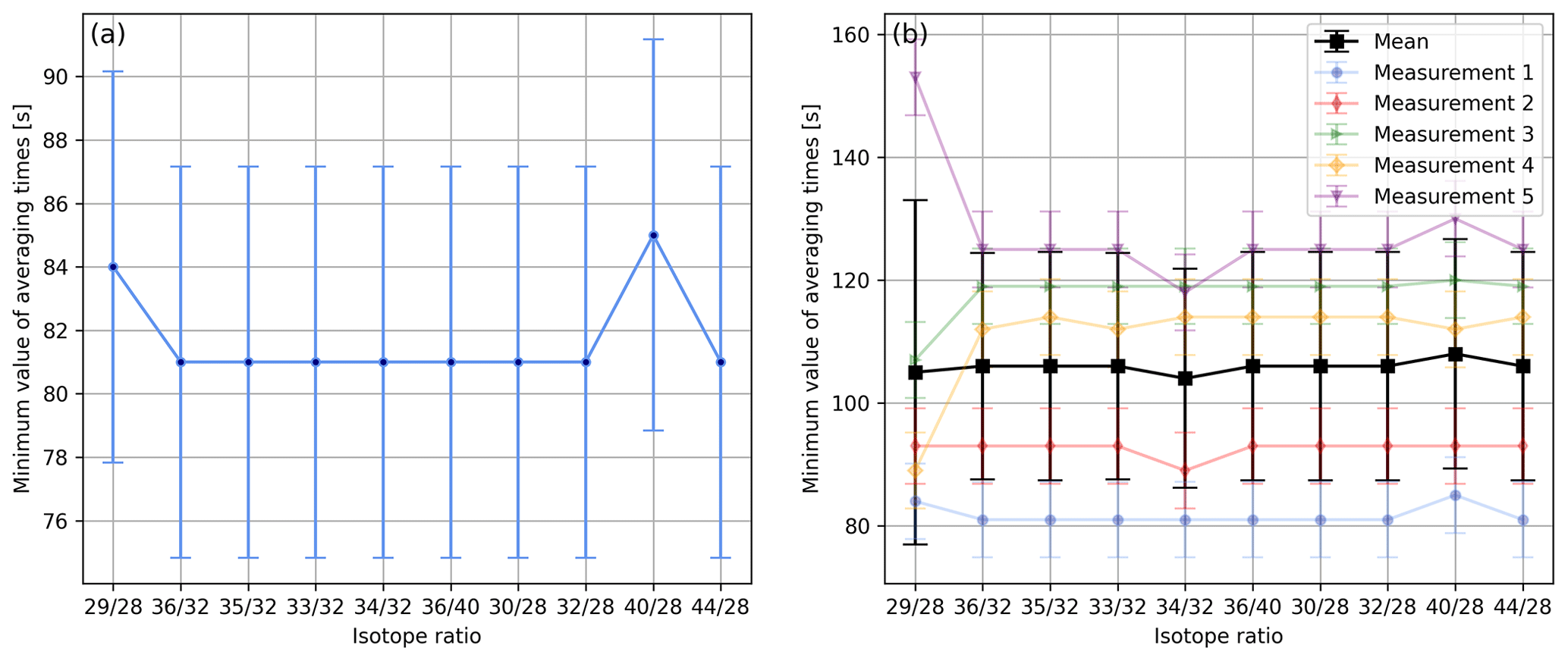
Figure 5(a) Minimum values of averaging times of different isotope ratios determined as indicated in Fig. 4; for the calculations the same data set was used as for Fig. 4. The uncertainty in each minimum was estimated by computing the standard deviation of the instants of time that were used for the calculation of the corresponding centred moving average. (b) Minimum values of averaging times of different isotope ratios calculated from five consecutive 1 h time scans of air (LUX 3588) following the procedure depicted in panel (a). Furthermore, panel (b) shows the mean values of the minima and the corresponding standard deviations.
3.4 Comparison of different inlet systems
Besides characterising the new measurement setup we also compared the NIS-II to other inlet systems, namely to an NIS-I, to an Elementar iso DUAL INLET and a dual-inlet system built by Thermo Finnigan. In contrast to the NIS-I and NIS-II, the latter two inlet systems are changeover-valve-based. In the following, we will compare measurement precisions of delta values of air components and focus on their reproducibility. The setups we used for these studies are the following:
- 1.
Elementar isoprime precisION with Elementar iso DUAL INLET
- 2.
Elementar isoprime precisION with the NIS-II (1)
- 3.
Thermo Finnigan DELTAplus XP with its integrated changeover-valve-based dual-inlet system
- 4.
Thermo Finnigan DELTAplus XP with the NIS-I
- 5.
Thermo Finnigan DELTAplus XP with the NIS-II (2).
The NIS-II systems that are part of setups 2 and 5 are two separate, identically built devices; therefore, they were numbered. However, in what follows, we drop these numbers for the sake of simplicity.
3.4.1 Comparison of open-split-based dual-inlet systems
In order to compare the NIS-II to the NIS-I we calculated correlations of internal and external precisions of various delta values of air components (see Fig. 6). The delta values were all measured with a Thermo Finnigan DELTAplus XP IRMS on air cylinders LUX 3407 (sample) and SC 560962 (standard). Please note that delta values calculated from measurements with the Thermo Finnigan DELTAplus XP are calculated as described in Appendix A, except that only consecutive standard intervals are averaged, whereas consecutive sample intervals are not; furthermore, to these data a 2.5σ filter is applied, and, normally, and are corrected for the drift of the standard gas.
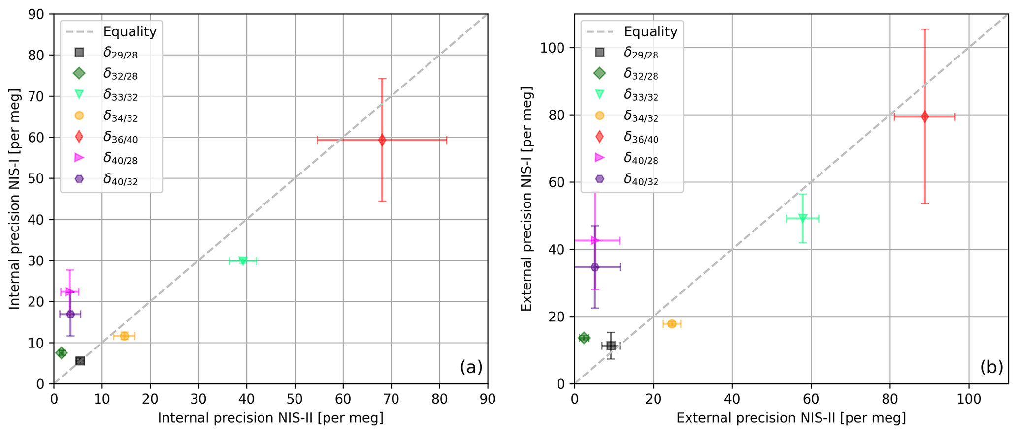
Figure 6(a) Internal and (b) external precisions of various delta values of air components (sample cylinder LUX 3407 and standard cylinder SC 560962). For the measurements a Thermo Finnigan DELTAplus XP with an NIS-I and an NIS-II was used; per inlet system, 50 measurements (8 delta values per measurement) were performed. The data were processed with a 2.5σ filter, and and were corrected for the drift of the standard gas. The error bars indicate the standard deviations of external and internal precisions, respectively; these precisions were calculated from three individual measurement series that were carried out on 3 different days. Each of these series consists of 10 consecutive measurements with 8 delta values per measurement.
From Fig. 6 it can be seen that delta values of air components can be measured with very high precisions when an open-split-based dual-inlet system is used; in general, these precisions are of the order of tens of per meg and higher. Moreover, the data imply that for most of the delta values the NIS-II and the NIS-I provide similar results. For the internal precisions, the largest absolute differences in the 50 measurements are 19 per meg (), 13 per meg () and 9 per meg (); for the former two delta values, the NIS-II was superior. Regarding external precision, and showed the largest discrepancies again; for these delta values, the NIS-II outperformed the NIS-I by 37 and 30 per meg, respectively. Since the comparison of measurements carried out on different days led to similar results (see error bars of Fig. 6), we conclude that the modifications we made to the NIS-I had a positive influence on the measurement precision.
3.4.2 Comparison of open-split-based to changeover-valve-based dual-inlet systems
When using changeover-valve-based dual-inlet systems, it can be observed that the beam intensity declines as a function of time. When a single SA–STD measurement of compressed air is carried out with the Elementar iso DUAL INLET, this decrease usually presents itself as depicted in Fig. 7a. The origin of this decline is the steady consumption of gas, which results in a gradual reduction in the gas pressure inside the bellows. Moreover, Fig. 7a makes it clear that the signals of the gas stored in the two bellows decrease differently. One reason for this is that the reference bellow is larger than the sample bellow (100 mL versus 40 mL), and the other is that the corresponding feeding capillaries are crimped similarly but not identically (see Sect. 3). To prevent this decrease from propagating further, before each individual measurement of a measurement series, the bellows are autobalanced with respect to a predefined signal height; for air and oxygen measurements this autobalancing is performed with respect to the and signals, respectively.
In contrast, Fig. 7b points out that data gathered with the NIS-II do not show a signal decrease. The NIS-II was designed in such a way that cylinders for sample and standard gas can be directly connected to the inlet system; since the gas pressure of the NIS-II is regulated, the signals remain approximately constant. Nevertheless, if small volumes of gas have to be measured, the amount of gas has to be sufficiently large to allow for a thorough purging of the open split (see Sect. 3.2); moreover, an MFC has to be added between the NIS-II and the gas container to stabilise the flow rate.
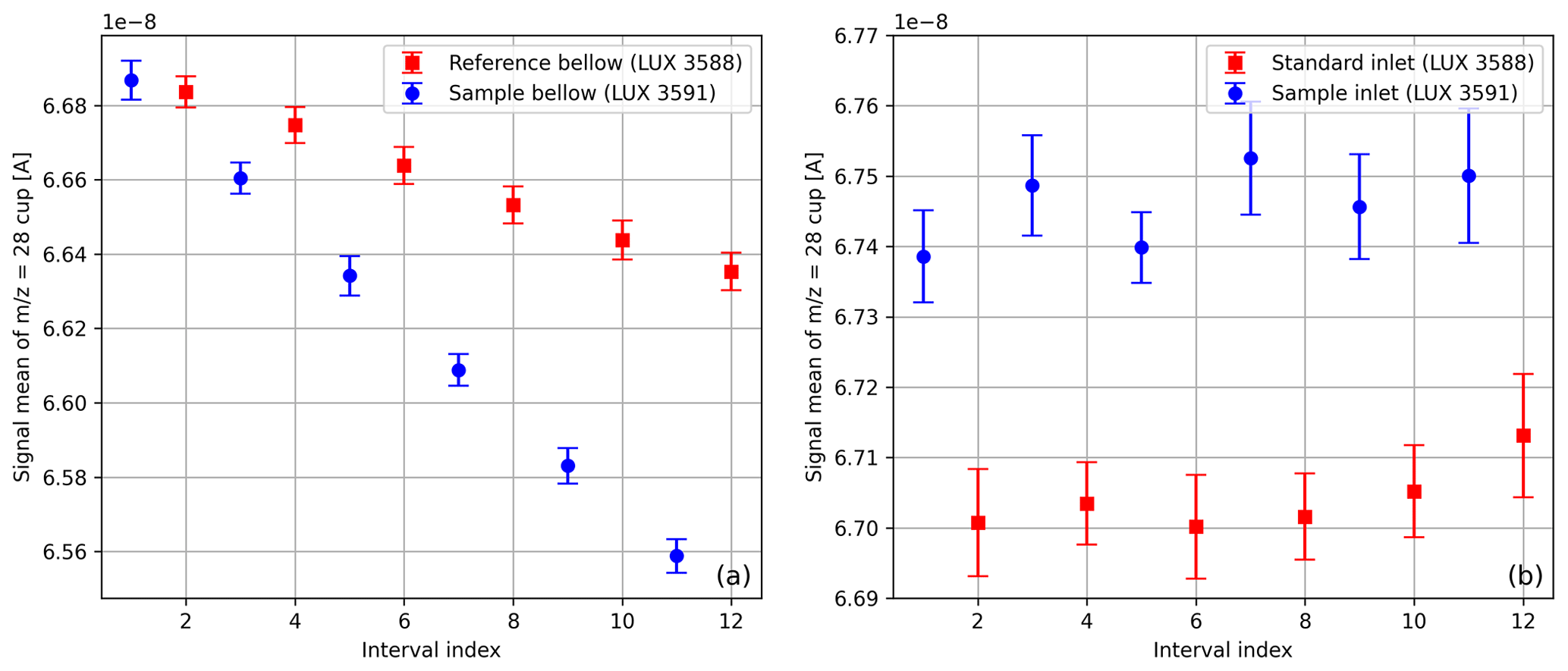
Figure 7Average signals of the cup with standard deviations; these values were determined from SA–STD measurements of compressed air (LUX 3588 and LUX 3591) with 12 measuring intervals per measurement. The measurement depicted in panel (a) was carried out with the iso DUAL INLET, and the one shown in panel (b) was done with the NIS-II.
Due to the previously mentioned observations, we correct data collected with conventional dual-inlet systems for non-linearity; this correction is necessary because our mass spectrometers were tuned with respect to maximum sensitivity instead of linearity. We apply the correction either to the interval means provided by the mass spectrometers' operating systems or directly to the ion beam data (typically 0.1 s resolution). In either case, we assess the decrease in the signals of sample and standard gas based on the signals; then we correct the isotope ratios or delta values accordingly. For the signal decrease, we always use a linear model and drop outliers if necessary; normally, our target is to obtain coefficients of determination of at least 0.7. When computing isotope ratios, delta values and their uncertainties, we follow the principles stated in Appendix A.
To compare the NIS-II to changeover-valve-based dual-inlet systems, we measured and on air (cylinders LUX 3588 and LUX 3591) with different setups (see introduction of this section); the results of this comparison are shown in Table 2. In the measurement series performed with the Thermo Finnigan DELTAplus XP and the NIS-II, the aforementioned gas cylinders were not measured directly against each other but against the same in-house standard; then the delta values referring to LUX 3591 (sample) against LUX 3588 (standard) were calculated from these data. For the evaluation of measurements with the DELTAplus XP and the NIS-II, 94 delta values from 13 SA–STD measurements were taken into consideration. The analysis of measurements performed with the DELTAplus XP and its integrated dual-inlet system was performed based on 100 delta values from 10 consecutive SA–STD measurements; in principle, this is also valid for measurements performed with the isoprime precisION, whereby the first two delta values of each measurement were dropped when the iso DUAL INLET was used. The reason for this is that most of these values turned out to be outliers. Outliers were also filtered when the DELTAplus XP was used with the NIS-II; to these measurements, we applied a 2.5σ filter. All of the measurements were carried out with an integration time of 20 s, except for those with the DELTAplus XP and the NIS-II; for this setup, the integration time was 10 s.
Table 2Mean values of and along with external precisions measured on compressed air (standard cylinder LUX 3588 and sample cylinder LUX 3591). These delta values were obtained with an Elementar isoprime precisION and a Thermo Finnigan DELTAplus XP (measurement and data processing procedures as described in the main text); as inlet systems an NIS-II, an Elementar iso DUAL INLET and a conventional dual-inlet system integrated into the DELTAplus XP were used. For the latter two inlet systems autobalancing was enabled. The non-linearity correction applied to some data sets involves a correction of the signal drift as well as of the remaining time dependence.
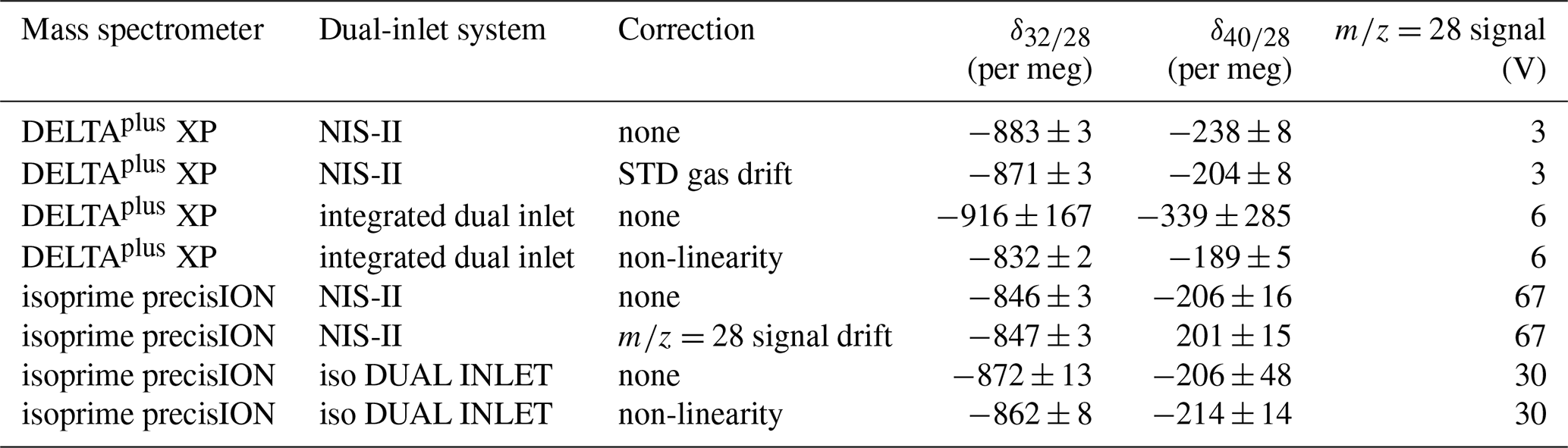
From Table 2 it is evident that the external precisions of delta values recorded with the NIS-II hardly change if drift corrections are applied; applying non-linearity corrections to data recorded with conventional dual-inlet systems must be taken into consideration, though. However, as will be shown in Sect. 3.4.3, such corrections do not always improve the results.
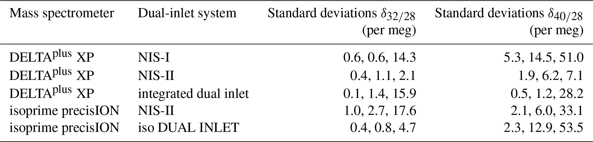
On the one hand, from Table 2, it can be seen that the Elementar isoprime precisION along with the NIS-II provided a distinctly higher precision for than with the iso DUAL INLET, namely 3 per meg instead of 8 per meg. On the other hand, measurements with the DELTAplus XP along with its integrated dual-inlet system led to higher precisions than those with the NIS-II; if a non-linearity correction is applied to the former data, the differences between the external precisions of and turn out to be 1 and 3 per meg, respectively. However, when looking at the standard deviations of mean values presented in Table 3, which shows 3 d reproducibilities, the NIS-II provided superior results than the integrated dual inlet. While the reproducibilities with the NIS-II are of the order of a few per meg, those of the integrated inlet system are of the order of tens of per meg.
When looking at the reproducibilities of delta value means recorded with the isoprime precisION, it is noticeable that the reproducibilities of the NIS-II data are also of the order of tens of per meg, though. Furthermore, it is striking that the reproducibilities of means recorded with the iso DUAL INLET are distinctly lower than those of the NIS-II. However, it must be taken into consideration that the former reproducibilities were determined from data recorded on 3 consecutive days, while the period between the NIS-II data sets was up to 2 years.
Another interesting feature of Table 3 regards the two open-split-based dual-inlet systems; in general, the results of the NIS-II turned out to be more reproducible. Especially the reproducibilities of the mean values seem to be higher, namely by over 10 per meg.
As an aside, it may be mentioned that the discrepancies of most of the corrected delta value means presented in Table 2 are within the measurement uncertainties shown in Table 3 (1σ of means); the difference in means recorded with the DELTAplus XP might be significant, though. However, it must be taken into account that with the NIS-II the gases LUX 3588 and LUX 3591 were not directly measured against each other. Moreover, the measurements with the different inlet systems were carried out at different signal intensities; this leads to non-linearity effects that have not been corrected. With the DELTAplus XP and its integrated dual-inlet system, we performed a measurement series during which the signal was varied between 2 and 8 V; the external precision of the corrected data recorded during this series was around 50 per meg (25 measurements with 12 delta values per measurement).
Table 3Reproducibilities of mean values as well as of internal and external precisions of and . Measurements with the DELTAplus XP along with the open-split-based dual-inlet systems were performed on air cylinders LUX 3407 (SA) and SC 560962 (STD); with the remaining setups, LUX 3591 (SA) was measured against LUX 3588 (STD). On 3 different days, three measurement series comparable to those presented in Table 2 were performed; after calculating the means and precisions of each series, the standard deviations of these values were computed. In the last two columns, the values are listed in the following order: standard deviation of internal precisions, standard deviation of external precisions and standard deviation of mean values (similar to external precision but for three measurement series carried out on different days). Measurements performed with conventional dual-inlet systems were corrected for non-linearity and the remaining time dependence. The data collected with the Thermo Finnigan DELTAplus XP and the open-split-based dual-inlet systems were corrected for the drift of the standard gas; additionally, a 2.5σ filter was applied to these data.
3.4.3 Influence of corrections and the idle time on measurement precisions
Besides the measurement precisions themselves, also the measurement durations and corrections required to achieve these precisions have to be taken into account; we studied this using the NIS-II and the Elementar iso DUAL INLET along with the Elementar isoprime precisION. For each inlet system, we performed 10 SA–STD measurements of compressed air. Since an additional standard gas interval was measured with the NIS-II, the first delta value of each individual measurement was dropped; by doing this, the same number of delta values is obtained for both measurement series. From the collected data we determined internal and external precisions of various delta values and evaluated them for two different idle times (switch delays); the actual idle time of the measurements was around 60 s, and then we reduced it to roughly 20 s using a processing feature of IonOS. The outcome of this study is depicted in the two panels of Fig. 8.
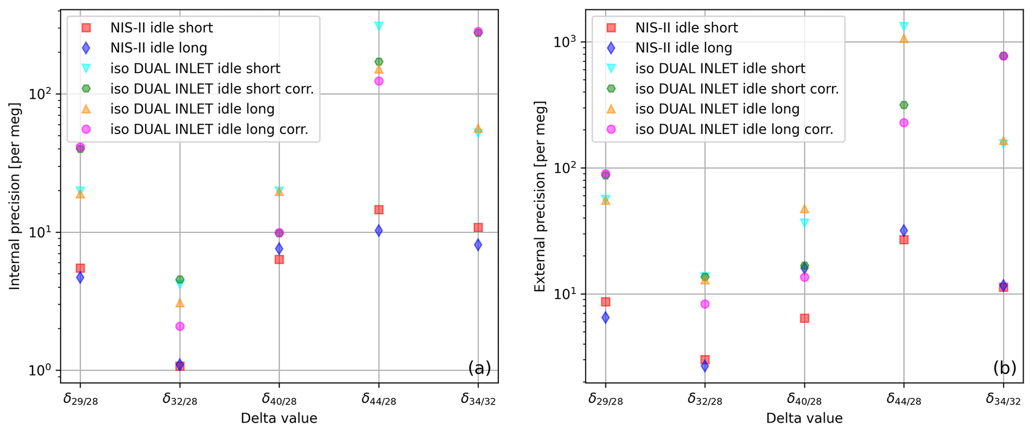
Figure 8(a) Internal and (b) external precisions of different delta values calculated from 10 SA–STD measurements of air (standard LUX 3588 and sample LUX 3591) performed with the Elementar isoprime precisION; as inlet systems the iso DUAL INLET and the NIS-II were used. Before each measurement with the iso DUAL INLET, the system autobalanced the signal. Data labelled as “corr.” were corrected for non-linearity and the remaining time dependence. The labels “idle short” and “idle long” refer to idle times of around 20 and 60 s, respectively.
The air data shown in Fig. 8 point out that the NIS-II is able to provide higher precisions than the iso DUAL INLET for various delta values; for these data, the only exception is measured with an idle time of around 60 s. Moreover, this measurement series suggests that the biggest differences between the two inlet systems might regard and .
Moreover, from Fig. 8 it can be seen that the precisions of the two inlet systems are still appreciably different even if non-linearity corrections are applied to the iso DUAL INLET data; in addition, the corrected and values imply that such corrections do not always improve the precisions. Non-linearity corrections only work well if there is a clear trend and little scattering. Thus, if the sample amount is vast, we prefer measuring with the NIS-II, whose data do not have to be corrected for non-linearity.
According to Fig. 8, for most of the delta values measured with the iso DUAL INLET an idle time of around 60 s led to higher internal precisions than an idle time of 20 s; it is less clear for external precisions, though. Concerning NIS-II data, in three out of five cases, the longer idle time led to higher precisions.
When conventional dual-inlet systems are used, the pressure in the ion source slightly changes when the gas source is switched; as a consequence, the system needs time to re-equilibrate. In contrast, with our open-split-based systems, the pressure in the ion source remains constant. Therefore, in some cases, measurements with the NIS-II can be carried out faster and at a higher precision than measurements with the iso DUAL INLET.
Due to the fact that with the NIS-II many delta values can be measured more precisely, more measurements have to be carried out with the iso DUAL INLET to obtain comparable precisions; this in turn translates into an additional expenditure of time. For instance, for measurements of with the iso DUAL INLET, a measurement series consisting of 10 SA–STD measurements would have to be repeated almost twice (calculation based on Table 2) to obtain comparable standard errors.
3.5 Feasibility study of clumped-isotope measurements of air components
As stated in the Introduction, one of our main goals was to determine whether our measurement setup allowed us to measure clumped isotopes of air components or not. In general, for such measurements the following requirements have to be met (Eiler, 2007).
-
High mass resolution. Mass spectrometers with a low mass resolution may not be able to resolve isobaric interferences. In some cases, high mass-resolving power can be compensated by high sample purity.
-
High abundance sensitivity. The abundance of clumped isotopes is typically much smaller than the abundance of singly substituted isotopologues, and thus a high abundance sensitivity is required.
-
High measurement precision. Typically, the required measurement precision is of the order of 10−5 and higher.
-
Preservation of the original molecular bonds. Alteration of molecular bonds during the measurement procedure or sample handling may modify the clumped-isotope signals.
In the following discussion, we only touch upon the first three of these basic requirements because they are directly related to the mass spectrometer and its inlet system. In contrast, the integrity of the original bonds also depends on other factors.
3.5.1 Mass resolution
Since the mass resolution of the Elementar isoprime precisION is merely around 110 m Δ m−1 (Elementar Analysensysteme GmbH, 2022), resolving isobaric interferences is not possible. For instance, Laskar et al. (2019) use a Thermo Scientific 253 Ultra High Resolution (HR) IRMS with a medium mass resolution of 10 000 m Δ m−1 to discriminate between 36Ar, H35Cl and 18O18O. Although air measurements with the isoprime precisION produce a well-defined peak, it is not possible to tell these three components apart, though. It is also not possible to distinguish clumped isotope 17O17O from the singly substituted isotopologue 16O18O or17O18O from 35Cl.
Due to the limited mass resolution of our IRMS, we concluded that the feasibility study regarding clumped-isotope measurements of air components cannot be focused on air but must be performed on the pure gases air is composed of. In what follows, we present measurements of pure-oxygen gas; we decided to focus on oxygen because it has multiple clumped isotopes and because our Faraday collector array has all of the required cups. In addition, clumped-isotope measurements of oxygen have already been published by other groups such that comparisons can be drawn.
As an aside, it may be mentioned that also molecular nitrogen was a potential candidate for our study because the abundance of 15N15N in N2 is more than 3 times higher than the abundance of 18O18O in O2 (Meija et al., 2016). However, 15N15N is the only clumped isotope of nitrogen, which makes it less suitable for our purpose.
3.5.2 Abundance sensitivity
The AV scan depicted in Fig. 9a proves that our setup is sensitive enough to detect 17O18O () and 18O18O () in pure-oxygen gas. Nevertheless, if the collector zeros are subtracted from these signals (around A), they both become negative; this eventually leads to incorrect delta values. Hence, the collector zeros do not represent the correct background of these signals.
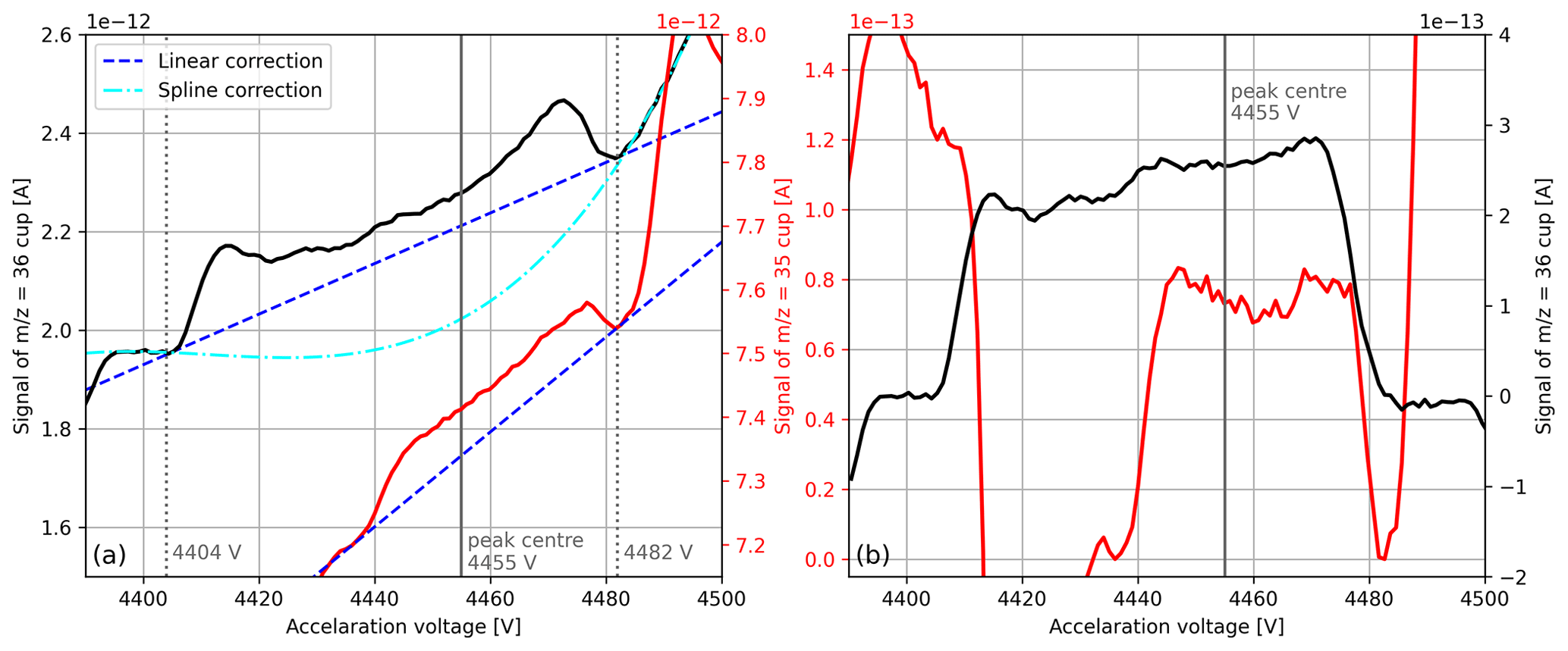
Figure 9(a) Raw signals of mass-to-charge ratios 35 and 36 around the measurement position (peak centre). The signals were both recorded during a single AV scan of pure-oxygen gas (cylinder SC 62349), which was performed with the isoprime precisION and the NIS-II. Besides the peak centre, suitable positions for background corrections (dotted lines) and the corresponding correction functions are indicated. (b) Corrected signals of mass-to-charge ratios 35 and 36. For the former signal, the linear correction depicted in panel (a) was used, and for the latter the spline correction was used.
On Faraday cups measuring clumped isotopes usually a negative background is visible, which is created by secondary electrons (Bernasconi et al., 2013). Furthermore, it is known that this background can lead to non-linearity effects and that the number of secondary electrons is positively correlated with the amount of gas that is admitted to the mass spectrometer (Bernasconi et al., 2013). In order to reduce this background we connected an external power supply to our IRMS and applied a suppressor voltage of −140 V to its Faraday cups. By default, this voltage is set to approximately −38 V (Elementar Analysensysteme GmbH, 2017). Measurements with the isoprime precisION have shown that the application of a much more negative voltage does not make sense because the signals start to saturate at around −100 V. At −100 V, the peak top signal of the cup was approximately 5 times higher than at −5 V (raw signal of A instead of A). Unfortunately, the application of a suppressor voltage alone is not enough to generate positive and signals. As suggested by Bernasconi et al. (2013), in order to solve this issue a background value in the presence of the analyte has to be determined.
One option presented by Bernasconi et al. (2013) is to infer the background from the main mass component of the analyte gas ( for oxygen). To determine the relationships between different Faraday cup signals at different acceleration voltages and at varying pressure levels, we carried out a series of AV scans. For this measurement series, we filled the reference bellow of the iso DUAL INLET with pure oxygen (SC 540546), maximised the signal through bellow compression and then performed an AV scan every 30 min without readjusting the bellow. To measure over a considerable range of source pressures, these scans were performed for 3 d; in this period, the signal declined from approximately to A.
To estimate the background of the peak we first inspected the AV scans to determine positions that represent the background appropriately. Because the peak was not flat but growing as a function of the acceleration voltage, we selected two positions, namely one before the peak and one after it (see Fig. 9a). By means of correlation plots created based on the AV scans, we then inferred the signal at these two positions from linear fits; as a predictor, we first tested the peak centre (measurement position) of the signal, which provided coefficients of determination of around 0.996. After linearly interpolating the two background values and subtracting the value at the peak centre from the signal, we eventually obtained a positive value. During regular SA–STD measurements this correction is applied to the individual interval means after the collector zero correction has been removed.
Later, we tested other correlations as well and noticed that using the peak centre of the signal as a predictor for the background provides not only better fits (R2≈0.99993) but also better results in terms of the accuracy of isotope ratio . Please note that the signal was still corrected by subtracting the collector zero value; the justification for this is that the signal ( A) is distinctly higher than the collector zero value ( A).
We repeated the same correction procedure for , and also here the peak centre of the signal predicted its background the best. However, as can be seen from Fig. 9a, for the linear correction is not ideal because the peak top is not flat. To take the curvature of the peak top into account, we calculated an appropriate spline. Instead of repeating this calculation for every SA–STD measurement we compute the linear correction for each of its interval means and then improve the correction by adding a constant value; this value, which corresponds to the difference between the spline and the linear correction, is deduced from a single AV scan (see Fig. 9b). To monitor the background of the peaks, before each measurement series an AV scan is performed; when major changes are observed, the corrections are recalculated.
3.5.3 Measurement precision
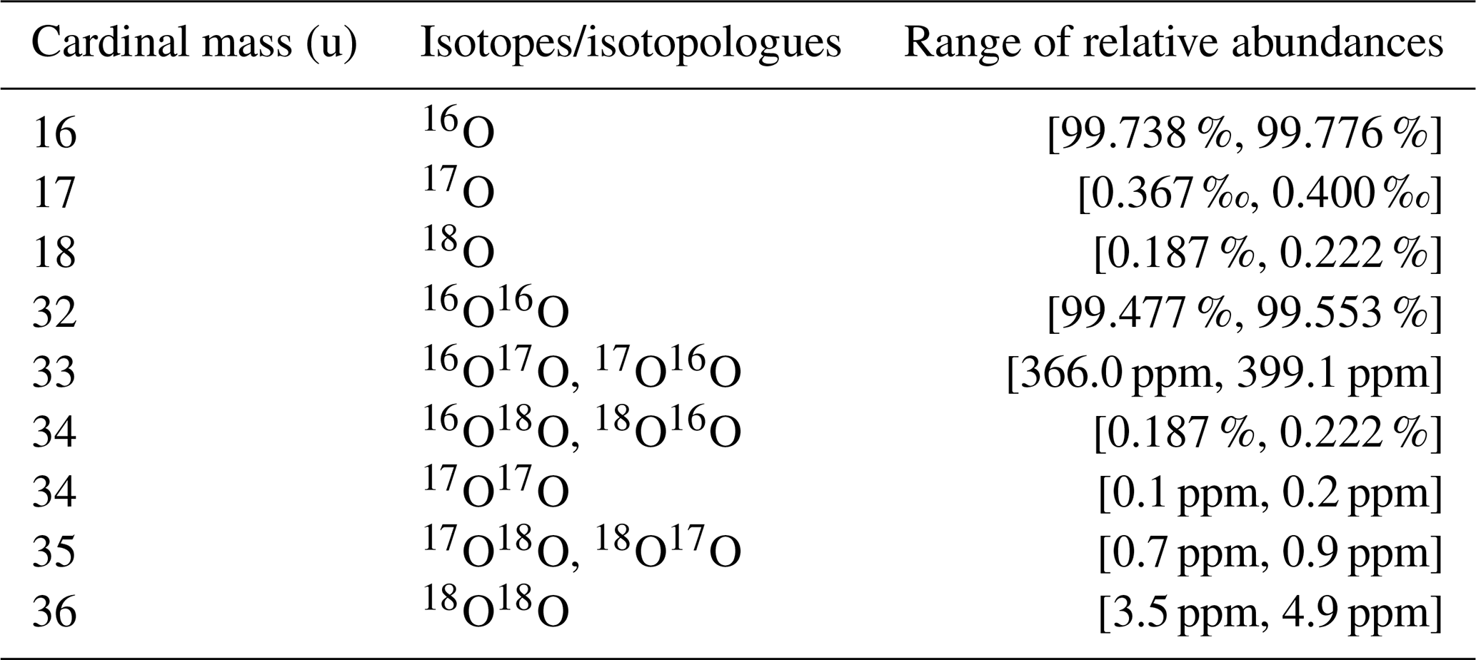
Since oxygen has two heavy isotopes, namely 17O and 18O, any combination of these isotopes is a clumped isotope of molecular oxygen. In Table 4 ranges of oxygen isotope abundances observed in natural materials are shown as well as the corresponding abundances of oxygen isotopologues.
Since oxygen isotope ratios are calculated with respect to 16O16O, whose relative abundance is almost equal to 1, the minimum measurement precision that is required to detect a certain isotope ratio is very similar to the relative abundance of the rare isotope. This implies that for isotope ratios and external precisions of at least and , respectively, have to be achieved (see Table 4).
Table 4Ranges of oxygen isotope abundances observed in natural materials (Meija et al., 2016) along with abundances of oxygen isotopologues calculated from the observed oxygen isotope abundances (last six rows).
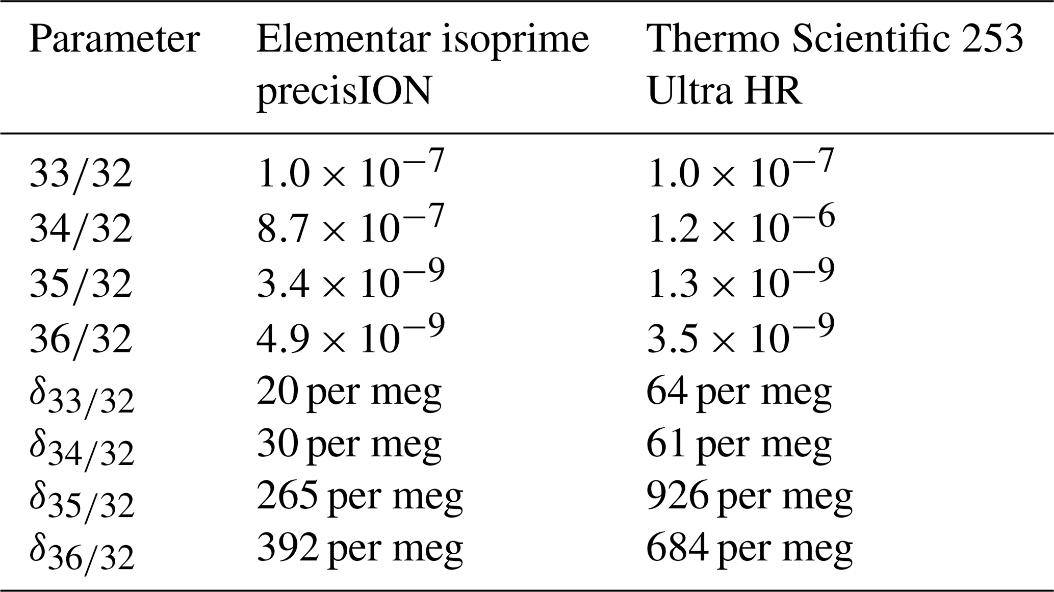
In Table 5 external precisions of oxygen isotope ratios and their delta values are shown; these were calculated from 10 SA–STD measurements of pure oxygen, which we performed with the isoprime precisION and the NIS-II. The signals were corrected using the collector zero value and the clumped-isotope signals according to the correlation method described in Sect. 3.5.2. When calculating the standard deviation of the 60 sample interval means, one obtains for and for ; hence, for these clumped-isotope ratios we have a resolving power of over 100.
Furthermore, in Table 5 we compare our measurements to those reported by Laskar et al. (2019) (their supplement), who performed clumped-isotope measurements on atmospheric oxygen with a Thermo Scientific 253 Ultra High Resolution IRMS. Except for isotope ratios and higher precisions were obtained with the Elementar isoprime precisION; for these ratios, the differences between the two mass spectrometers are relatively small, though, namely and , respectively. However, the integration time Laskar et al. (2019) used is 67 s and not 20 s.
Table 5Standard deviations of oxygen isotope ratios and delta values calculated from 60 independent interval means of pure-oxygen gas measurements. In the second column, data collected with the Elementar isoprime precisION and the NIS-II are shown; the precisions were calculated from 10 SA–STD measurements (sample cylinder SC 540546 and standard cylinder SC 62349), and the data were corrected as described in Sect. 3.5.2. In the third column, data published by Laskar et al. (2019) (their supplement) are presented. They measured purified oxygen (extracted from atmospheric air) against the working gas Institute for Marine and Atmospheric Research Utrecht (IMAU) O2 (Linde Gas, Schiedam, the Netherlands) with a Thermo Scientific 253 Ultra High Resolution IRMS. The reported precisions were calculated from 10 of these measurements, whereby pressure corrections were applied to and . The signal intensities of the Elementar isoprime precisION and the Thermo Scientific 253 Ultra HR were around and A, respectively.
The operation of the NIS-II for more than a year has shown that this dual-inlet system requires significantly less maintenance than the NIS-I; thanks to the new capillary switching mechanism and the straight open split, only very few hours have to be spent on maintenance per year. Furthermore, using a straight glass tube instead of a Y-shaped piece as an open-split interface is beneficial because installation is much faster and gas tightness is superior. However, when compared to the Y-shaped open split, the minimum purge flow rate of the new one is twice as high. As far as the measurement performance is concerned, our data indicate that the reproducibility of and mean values could be superior for the NIS-II.
Moreover, we compared the NIS-II to two different changeover-valve-based dual-inlet systems and demonstrated that data recorded with the former inlet system do not require non-linearity corrections; this makes it a highly reliable system because such corrections do not always lead to higher precisions. This advantage is at the expense of a significantly higher sample consumption, though.
By means of measurements of and on air, we also showed that 3 d reproducibilities of mean values recorded with the NIS-II over almost 2 years are of the order of tens of per meg at most. In addition, measurements performed with our Elementar isoprime precisION and Thermo Finnigan DELTAplus XP along with a NIS-II generally led to superior reproducibility compared to those with changeover-valve-based dual-inlet systems; we observed differences of up to 21 per meg (). The only exception was the measurement of performed with the Elementar isoprime precisION and the NIS-II; here, the difference was around 13 per meg.
Through measurements of isotope ratios and on pure-oxygen gas we also demonstrated that with the Elementar isoprime precisION and the NIS-II clumped-isotope studies on pure gases are feasible; for these two ratios, we attained precisions that are over 2 orders of magnitude higher than the required minimum values. In addition, we showed that in terms of precision, our setup can keep up with the Thermo Scientific 253 Ultra High Resolution IRMS. Due to the low mass resolution of the Elementar isoprime precisION and the existence of isobaric interferences, though, clumped-isotope measurements can only be performed on pure gases or gas mixtures without isobaric interferences.
Currently, we mainly use the NIS-II to measure and on ambient air samples with precisions at the scale of per meg. Due to the auspicious results regarding clumped-isotope measurements, we are planning to use the NIS-II to measure clumped isotopes of O2, N2 and CO2. However, to make such measurements possible, more work has to be done. Currently, we are attempting to perform clumped-isotope measurements on pure-oxygen gas according to common practices; moreover, we are improving our background correction routine because the mean values of oxygen isotope ratios and still lack proper calibration.
The software of the Elementar isoprime precisION, IonOS, calculates delta values by making use of three consecutive isotope ratio means; on the condition that an SA–STD measurement is composed of 12 measuring intervals (6 standard and 6 sample measurements performed in alternating order) and that the resulting isotope ratios means are denoted by Ri (), the first delta value is calculated as follows:
In analogy to the first delta value, the second one is given by
The delta values of the subsequent measuring intervals are computed accordingly.
When applying the propagation of uncertainty to Eq. (A1), one obtains the following expression for the uncertainty in δ1:
A repetition of this calculation for Eq. (A2) yields
In Eqs. (A3) and (A4), ΔRi denotes the uncertainty in the isotope ratio mean of the measuring interval i and ρR is the correlation coefficient (identical for all Δδi); for ρR we use the correlation between the six standard and the six sample ratios (averages of the mean sample and standard isotope ratios are taken into account).
Because IonOS does not provide the uncertainties in the isotope ratios ΔRi, we compute them with the help of the propagation of uncertainty as well. When denoting the signal area in the isotope ratios' numerator by Ai (uncertainty ΔAi), the one in its denominator by Bi (uncertainty ΔBi) and the correlation coefficient of these areas by , the uncertainty in isotope ratio is given by
For ΔAi and ΔBi we generally use standard deviations; for standard intervals (odd i) we calculate the standard deviation of the six standard interval areas and then repeat the calculation for the sample intervals (even i). Similarly, we only calculate one correlation coefficient per gas, namely by computing the correlation between the six Ai and the six Bi instances of the corresponding gas. Hence, not every ΔRi gets a different ΔAi, ΔBi and , but standard and sample intervals do.
The data and code are both available upon request (stephan.raess@unibe.ch).
SR was in charge of the investigation. PN and WP provided technical support. The formal analysis and validation of the thereby generated data were carried out by SR and MCL. PN and MS performed the measurements with the Thermo Finnigan DELTAplus XP; moreover, MS carried out the formal analysis of the data he collected. In the instrument development MCL, PN and various members of the workshop teams of the division of Climate and Environmental Physics of the University of Bern were involved. SR was in charge of visualisation and wrote the original draft of the paper. In the reviewing and editing process SR, MCL, PN and PW were involved. MCL and PW were responsible for funding acquisition.
The contact author has declared that none of the authors has any competing interests.
Publisher’s note: Copernicus Publications remains neutral with regard to jurisdictional claims made in the text, published maps, institutional affiliations, or any other geographical representation in this paper. While Copernicus Publications makes every effort to include appropriate place names, the final responsibility lies with the authors.
First of all, we would like to express our gratitude to Elementar Analysensysteme GmbH, Elementar-Straße 1, 63505 Langenselbold, Germany, and in particular Elementar UK Ltd., Isoprime House, Earl Road, Cheadle Hulme, Stockport, SK8 6PT, United Kingdom, which provided technical support for this work. Samples for clumped isotopes will be facilitated by the flask sampler run by the ICOS-CH project (no. SNF-20FI20_198227). Furthermore, we would like to sincerely thank the members of the workshop teams of the division of Climate and Environmental Physics of the University of Bern, whose effort regarding the design, development and maintenance of the open-split-based dual-inlet system was indispensable. Last but not least a special thank you goes to Michael Schibig, who performed and evaluated measurements with the Thermo Finnigan DELTAplus XP.
This research has been supported by the Swiss National Science Foundation (SNF; project no. 172550) and by a research agreement between Elementar Analysensysteme GmbH and the University of Bern (2020).
This paper was edited by Thomas Röckmann and reviewed by three anonymous referees.
Allan, D. W.: Statistics of atomic frequency standards, P. IEEE, 54, 221–230, https://doi.org/10.1109/PROC.1966.4634, 1966. a
Berhanu, T. A., Hoffnagle, J., Rella, C., Kimhak, D., Nyfeler, P., and Leuenberger, M.: High-precision atmospheric oxygen measurement comparisons between a newly built CRDS analyzer and existing measurement techniques, Atmos. Meas. Tech., 12, 6803–6826, https://doi.org/10.5194/amt-12-6803-2019, 2019. a
Bernasconi, S. M., Hu, B., Wacker, U., Fiebig, J., Breitenbach, S. F., and Rutz, T.: Background effects on Faraday collectors in gas‐source mass spectrometry and implications for clumped isotope measurements, Rapid Commun. Mass Sp., 27, 603–612, https://doi.org/10.1002/rcm.6490, 2013. a, b, c, d
Brand, W. A.: PreCon: a fully automated interface for the Pre-Gc concentration of trace gases on air for isotopic analysis, Isot. Environ. Healt. S., 31, 277–284, 1995. a
Eiler, J. M.: “Clumped-isotope” geochemistry – The study of naturally-occurring, multiply-substituted isotopologues, Earth Planet. Sc. Lett., 262, 309–327, https://doi.org/10.1016/j.epsl.2007.08.020, 2007. a, b
Elementar Analysensysteme GmbH: isoprime precisION User Manual A comprehensive user manual describing how to work with an isoprime precisION system, http://support.elementar.co.uk/documentation/Subsystems/precisION/manuals/ (last access: 5 September 2017), 2017. a
Elementar Analysensysteme GmbH: isoprime precisION The most flexible IRMS ever created, Art.-No. 05 005 646, 03/2022 A, https://www.elementar.com/de/produkte/stabilisotopenanalysatoren/massenspektrometer/isoprime-precision (last access: 4 April 2022), 2022. a
Laskar, A. H., Peethambaran, R., Adnew, G. A., and Röckmann, T.: Measurement of 18O18O and 17O18O in atmospheric O2 using the 253 Ultra mass spectrometer and applications to stratospheric and tropospheric air samples (including supplement), Rapid Commun. Mass Sp., 33, 981–994, https://doi.org/10.1002/rcm.8434, 2019. a, b, c, d
Leuenberger, M., Nyfeler, P., Moret, H. P., Sturm, P., and Huber, Ch.: A new gas inlet system for an isotope ratio mass spectrometer improves reproducibility, Rapid Commun. Mass Sp., 14, 1543–1551, https://doi.org/10.1002/1097-0231(20000830)14:16<1543::AID-RCM62>3.0.CO;2-H, 2000. a, b, c, d, e, f, g, h, i, j
Leuenberger, M. C., Schibig, M. F., and Nyfeler, P.: Gas adsorption and desorption effects on cylinders and their importance for long-term gas records, Atmos. Meas. Tech., 8, 5289–5299, https://doi.org/10.5194/amt-8-5289-2015, 2015. a
Meija, J., Coplen, T. B., Berglund, M., Brand, W. A., De Bièvre, P., Gröning, M., Holden, N. E., Irrgeher, J., Loss, R. D., Walczyk, T., and Prohaska, T.: Isotopic compositions of the elements 2013 (IUPAC Technical Report), Pure Appl. Chem., 88, 293–306, https://doi.org/10.1515/pac-2015-0503, 2016. a, b