the Creative Commons Attribution 4.0 License.
the Creative Commons Attribution 4.0 License.
 | 12 Oct 2023
The SPARC water vapour assessment II: biases and drifts of water vapour satellite data records with respect to frost point hygrometer records
Michael Kiefer
Dale F. Hurst
Gabriele P. Stiller
Stefan Lossow
Holger Vömel
John Anderson
Faiza Azam
Jean-Loup Bertaux
Laurent Blanot
Klaus Bramstedt
John P. Burrows
Robert Damadeo
Bianca Maria Dinelli
Patrick Eriksson
Maya García-Comas
John C. Gille
Mark Hervig
Yasuko Kasai
Farahnaz Khosrawi
Donal Murtagh
Gerald E. Nedoluha
Stefan Noël
Piera Raspollini
William G. Read
Karen H. Rosenlof
Alexei Rozanov
Christopher E. Sioris
Takafumi Sugita
Thomas von Clarmann
Kaley A. Walker
Katja Weigel
Satellite data records of stratospheric water vapour have been compared to balloon-borne frost point hygrometer (FP) profiles that are coincident in space and time. The satellite data records of 15 different instruments cover water vapour data available from January 2000 through December 2016. The hygrometer data are from 27 stations all over the world in the same period. For the comparison, real or constructed averaging kernels have been applied to the hygrometer profiles to adjust them to the measurement characteristics of the satellite instruments. For bias evaluation, we have compared satellite profiles averaged over the available temporal coverage to the means of coincident FP profiles for individual stations. For drift determinations, we analysed time series of relative differences between spatiotemporally coincident satellite and hygrometer profiles at individual stations. In a synopsis we have also calculated the mean biases and drifts (and their respective uncertainties) for each satellite record over all applicable hygrometer stations in three altitude ranges (10–30 hPa, 30–100 hPa, and 100 hPa to tropopause). Most of the satellite data have biases <10 % and average drifts <1 % yr−1 in at least one of the respective altitude ranges. Virtually all biases are significant in the sense that their uncertainty range in terms of twice the standard error of the mean does not include zero. Statistically significant drifts (95 % confidence) are detected for 35 % of the ≈ 1200 time series of relative differences between satellites and hygrometers.
- Article
(31079 KB) - Full-text XML
-
Supplement
(3734 KB) - BibTeX
- EndNote


Water vapour is the most potent greenhouse gas in the atmosphere (Kiehl and Trenberth, 1997). Its radiative effect per unit mass change is strongest around the tropical tropopause (Riese et al., 2012; Solomon et al., 2010). Trends of stratospheric water vapour are expected to be related to the temperatures of the tropical tropopause where air transporting water vapour enters the stratosphere (e.g. Fueglistaler and Haynes, 2005; Randel and Park, 2019). Rising troposphere and tropopause temperatures due to global warming may lead to increasing stratospheric water vapour abundances, initiating a positive feedback loop where global warming will be further accelerated due to increasing water vapour abundances in the lower stratosphere (e.g. Gettelman et al., 2010; Dessler et al., 2013, 2016). In addition, the major stratospheric source of water vapour is the oxidation of methane (e.g. le Texier et al., 1988), which has more than doubled since 1800 (Blunier et al., 1993) and is expected to continue rising in future (e.g. Lelieveld et al., 1998), further increasing stratospheric water vapour.
Since 1980, despite constant or slightly decreasing tropical tropopause temperatures (Gettelman et al., 2009; Hu et al., 2015), an increase in stratospheric water vapour has been observed over Boulder, Colorado (Oltmans and Hofmann, 1995). This cannot be explained by the high positive correlation between tropical tropopause temperatures and water vapour in the lowermost tropical stratosphere (Fueglistaler and Haynes, 2005; Randel and Park, 2019). In consequence, numerous studies have been performed to better understand the stratospheric water vapour budget and trends (e.g. Oltmans and Hofmann, 1995; Oltmans et al., 2000; Rosenlof et al., 2001; Nedoluha et al., 2003; Hurst et al., 2011b; Dessler et al., 2014; Hegglin et al., 2014; Brinkop et al., 2016). Vertically resolved profiles of atmospheric water vapour have been observed around the globe by satellite-based instruments in low Earth orbits since the mid-1970s. From the year 2000 on, 15 different satellite instruments have observed vertically resolved water vapour distributions from the middle troposphere to the mesosphere and above. More than 2 decades ago, a first assessment of the quality of water vapour observations including ground-based, balloon-borne and satellite instrumentation was published as the WCRP/SPARC (World Climate Research Programme/Stratosphere-troposphere Processes And their Role in Climate) report no. 2 (Kley et al., 2000). The many new satellite instruments in orbit since 2000 have made it of great interest to reassess the quality and consistency of water vapour observations from space. Here we concentrate only on stratospheric measurements by satellites and balloon-borne frost point hygrometers (FPs).
Many of the satellite data records included in this study are described in detail by their data providers in reports and scientific papers (a compilation of information relevant to this paper is presented in Walker et al., 2023). These reports and scientific papers also contain, in most cases, some information about validation activities. Frost point hygrometers have often been used for satellite data validation since they are considered to be most accurate and internally consistent water vapour instruments for stratospheric measurements. Comparisons of different instruments, including their calibrations and data processing routines, were the focus of several field campaigns (Vömel et al., 2007a, b, 2016; Hurst et al., 2011a; Rollins et al., 2014; Hall et al., 2016). Despite differences between the measurements by instruments employing different sensing techniques, consistency was found within the data from FPs.
Each comparison of satellite data records to the FP soundings, however, has been done in a slightly different way by each validation team, resulting in a wealth of validation publications that are not consistent down to the last detail. This lack of consistency hampers activities where several satellite data records need to be merged to construct a long-term time series, e.g. for trend assessments. For this reason, we decided for this WCRP/SPARC WAVAS-II (Water Vapor Assessment II) activity to perform the comparison of all available satellite data records obtained during the period of 2000 through 2016 to FP data in a fully consistent and reproducible way. We document here where the FP data came from, how we made them comparable to the satellite data, and how the comparisons were performed. Overall, all of our satellite-to-FP comparisons are done in a similar way. The result of this activity is the first fully self-consistent quality assessment of vertically resolved biases and drifts in the stratospheric water vapour measurements by numerous satellite instruments and FPs, along with the respective uncertainties. In order to be consistent with the other assessments within the WCRP/SPARC WAVAS-II activity (see ACP/AMT/ESSD special issue “Water vapour in the upper troposphere and middle atmosphere: a WCRP/SPARC satellite data quality assessment including biases, variability, and drifts”, https://amt.copernicus.org/articles/special_issue10_830.html, last access: 28 September 2023), we use the same data versions as used in other papers in the WAVAS-II special issue, even in cases where newer data versions have become available in the meantime.
The paper is structured as follows: in Sect. 2 we describe the FP data and the satellite data records, including their preparation for use within this study. Further, we explain how we made the FP data comparable in terms of their vertical resolution and how the biases and the drifts have been calculated. Section 3 presents the assessment of the biases between the satellite and FP data records, starting with each individual satellite data record versus the FP data at each site and then discussing comparisons of all satellite data versus one station, as well as one satellite data record versus all stations. We summarize these findings with a synopsis of the biases and their uncertainties for each satellite data set over all its associated FP sites, in three different altitude ranges. Section 4 presents the assessment of instrumental drifts of the satellite data records against FP records, also including a synopsis of the drifts of each satellite data set, in three altitude ranges, over all its associated FP sites. Section 5 summarizes our findings and offers recommendations for the use of the satellite data records under assessment. The individual bias and drift figures for pairs of satellite records and FP stations are presented in the Supplement and Appendix to this paper, respectively.
In this study, we compare the satellite data records under assessment in the WCRP/SPARC WAVAS-II activity to reference-quality FP soundings at 27 stations (79∘ N to 45∘ S latitude) during 2000 through 2016. A total of 31 data records from 15 different satellite instruments provide a subset of measurements coincident with the FP soundings (for coincidence criteria see below) that can be evaluated against the profile data from FP balloon soundings. In the following, we briefly describe FP and satellite data, explain the adjustments of the vertical resolution of the FP data to each of the various satellite data records, and describe the methods for the bias and drift assessments.
2.1 Frost point hygrometer data
The chilled mirror technique (Brewer, 1949; Barrett et al., 1950) is based upon the well-known equilibrium thermodynamic relationship (Clausius–Clapeyron) between an ice or liquid water surface and overlying water vapour. Frost point hygrometers actively maintain the equilibrium of this two-phase system by continuously adjusting the temperature of the condensate layer such that it remains stable. Both the NOAA (National Oceanic and Atmospheric Administration) Global Monitoring Laboratory's frost point hygrometer (NOAA FPH) and the cryogenic frost point hygrometer (CFH) use optical detection of the condensate layer on a small mirror. A feedback loop actively regulates the mirror temperature to maintain a stable condensate layer, making the water vapour content of the overlying air directly calculable from the mirror temperature.
The balloon-borne NOAA FPH was first flown over Boulder, CO, in 1980 (Oltmans et al., 2000) and, to date, has produced a 43-year record of stratospheric water vapour mixing ratios (Hurst et al., 2011b). It has also been flown routinely at Lauder, New Zealand, since 2004 and Hilo, Hawaii, since 2010 and has been part of a number of tropical, mid-latitude, and polar measurement campaigns (Kley et al., 1997). The NOAA FPH payload is configured to enable measurements not only during ascent but also during controlled (5 m s−1) descent of the balloon when water vapour contamination is improbable. The FPH measurement uncertainty is largely determined by the stability of the frost layer and, under satisfactory performance, is 0.1–0.3 K in frost-point temperature in the stratosphere, leading to a measurement uncertainty of <6 % for stratospheric mixing ratios (Hall et al., 2016).
Table 1Overview of NOAA (National Oceanic and Atmospheric Administration) frost point hygrometer (NOAA FPH) and cryogenic frost point hygrometer (CFH) stations used for comparisons with satellite data.
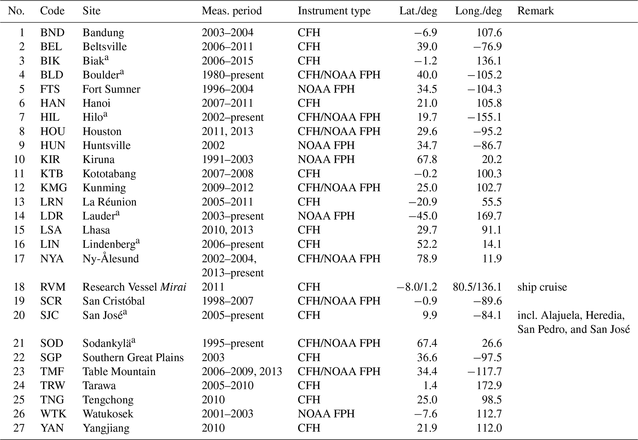
a Data from these sites were used for the drift analyses.
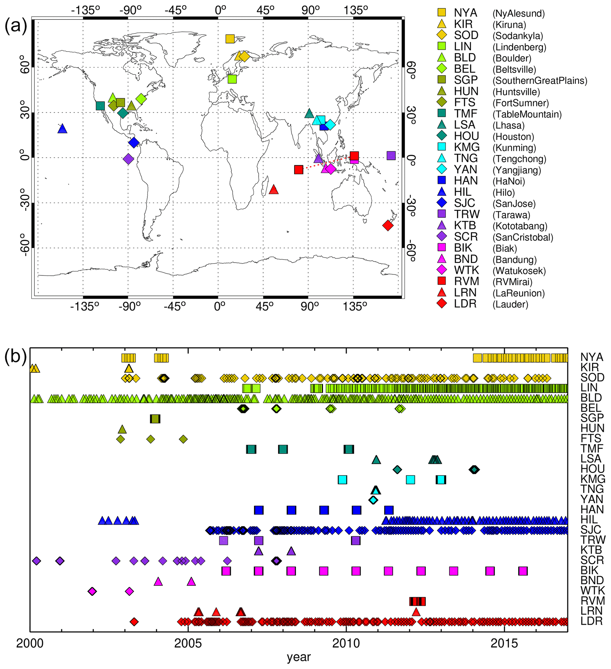
Figure 1Locations of NOAA FPH and CFH stations that provided measurement data for these intercomparisons (a) and the temporal coverage of the data records at the respective stations (b). RV Mirai was a measurement campaign based on a ship cruise. This is indicated by the dotted line connecting the respective symbols. In the lower plot each symbol represents at least one balloon-borne FP sounding. Note that some of the FP data sets began before 2000, but only the data from 2000 through 2016 are used here for bias and drift evaluations. FP record start dates are presented in Table 1.
The CFH (Vömel et al., 2007a, b, 2016) works along the same principle as the NOAA FPH but uses a proportional–integral–derivative controller with a continuously variable parameter schedule to make observations between the surface and the middle stratosphere (25 km). The uncertainty of the condensate phase in the temperature range below 0 ∘C is largely eliminated, allowing continuous profiles over a wider range of frost-point temperatures to be measured. It suffers no artefacts in cirrus clouds and may only be limited in wet precipitating clouds with the detector lens getting wet. The measurement uncertainty of the CFH is less than 0.5 K throughout the entire profile, which translates to conservative uncertainty values of 4 % in the lower troposphere and increasing to 9 % in the stratosphere.
Neither the CFH nor NOAA FPH requires water vapour calibration standards or a water vapour calibration scale; only the mirror thermistor must be calibrated with high accuracy, and this is accomplished using traceable standards of the US National Institute of Standards and Technology (NIST).
Temperature and pressure measurements used to convert frost point hygrometer data into relative humidity values and volume mixing ratios, respectively, are from the accompanying radiosondes on each balloon. Measurements of temperature and pressure have been provided by different radiosonde models throughout the years: Vaisala models RS80, RS92, and RS41; InterMet models iMet-1-RSB and iMet-4-RSB; and Meisei models RS-06G and RS-11G.
Offsets in the pressure measurements of radiosondes may bias the calculation of the mixing ratio in the stratosphere (Stauffer et al., 2014; Inai et al., 2015). To minimize this bias, the radiosonde pressure measurements are usually corrected using the radiosonde's acquisition of the geometric altitude by Global Navigation Satellite System (GNSS). In some radiosonde systems, the pressure is not measured directly but instead derived from the GNSS altitude. Only in older systems that precede the availability of GNSS observations on radiosondes starting in the late 1990s are pressures used without any corrections except those based on a simple pre-flight comparison at the surface with ground-based sensors. For this work we used FP mixing ratio averages on a fixed 250 m altitude grid. These are typically further reduced in vertical resolution as they are convolved with real or constructed averaging kernels for the different satellite instruments (see Sect. 2.3).
Table 1 lists the stations from which NOAA FPH or CFH data have been used for comparison with satellite data, together with their period of operation, the type of instrument launched, and the geographical coordinates of the site. Each station is given a three-letter code to simplify its identification in the remainder of this paper. Figure 1 provides an overview of the geographical locations and the measurement periods of the stations, together with the symbols and colour codes that are used throughout this paper to mark the respective data of the stations.
In the remainder of this paper we do not distinguish between NOAA FPH and CFH, so we continue to use the generic term “FP” for frost point hygrometer instruments and data.
2.2 Satellite data
Satellite data from all instruments providing measurements coincident with FP balloon soundings have been selected. Data quality filter criteria according to the original data descriptions from the data providers have been applied (for a summary of these data-set-specific criteria, see Walker et al., 2023). No further bulk screening for data outliers surviving the previous data quality filtering has been applied. The 31 satellite data records that are used in this comparison are listed in Table 2 along with their three-letter codes. Figure 2 shows the symbols and colour codes for the satellite data sets used throughout this paper. The data versions we have assessed in this study are not the most recent ones to date for most of the satellite data sets. For reasons of consistency, the data versions used here are the same as those assessed by the other comparative studies of the SPARC WAVAS-II activity. It is left to future studies to evaluate if more recent data versions of water vapour satellite data are improved with respect to those assessed here. Such evaluations can also be done individually by comparing newer data versions to those assessed here to quantify any changes in the biases and drifts reported here.
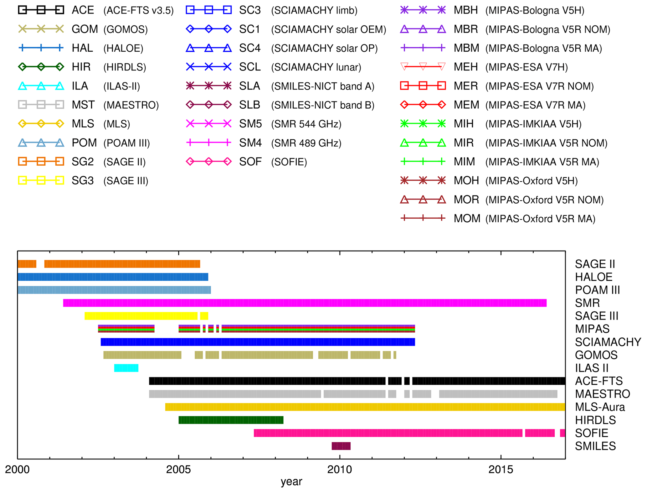
Figure 2Colours, symbols, and three-letter codes for the satellite data records used throughout the paper (upper part) and temporal distribution of available data of the respective satellite instruments on a monthly basis until the end of 2016 (lower part, not divided into measurement modes or data versions). Note that three of the SAT data sets began before 2000 (SAGE II 1984, HALOE 1991, POAM III 1998), but only the data from 2000 through 2016 are used here for bias and drift evaluations.
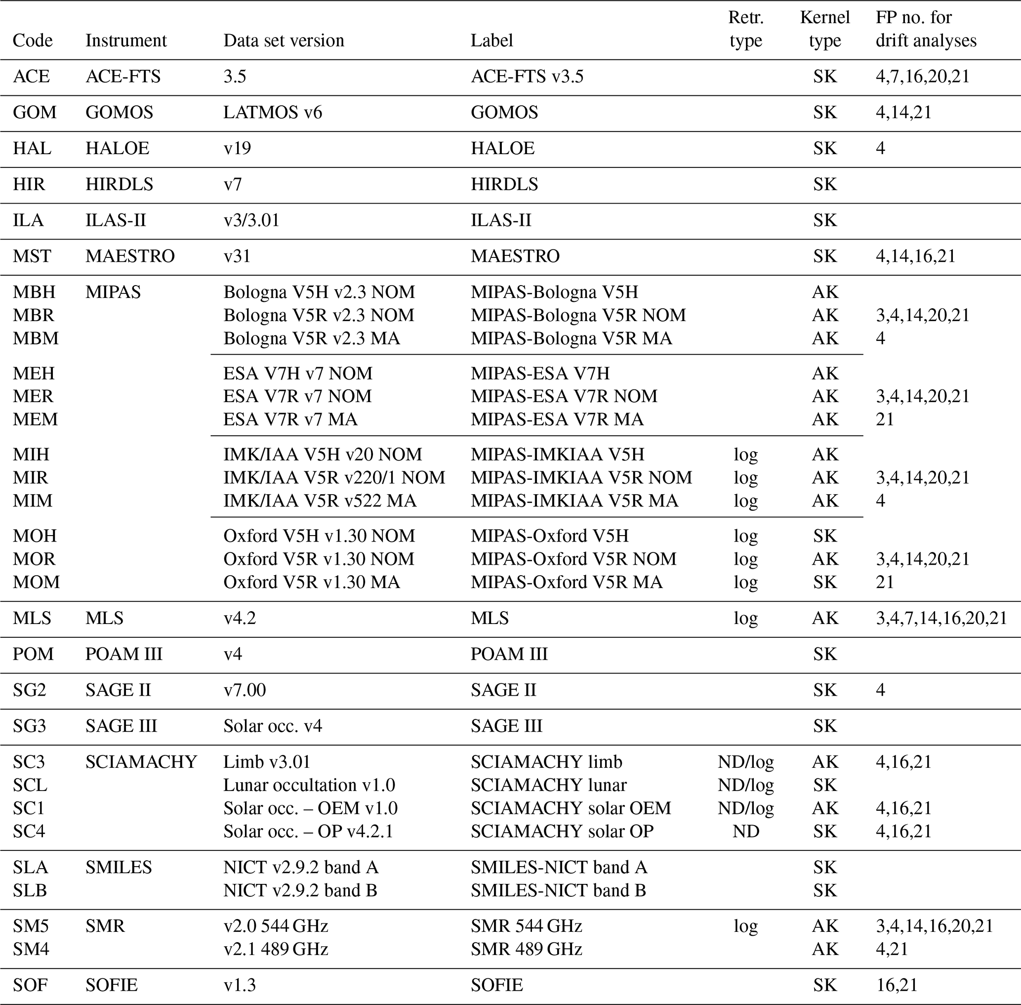
Table 2Overview of the water vapour data sets from satellites used in this study. Column “Retr. type” indicates whether the retrieval result was number density (marked ND) instead of VMR and whether the retrieval was done in the log (vmr) or domain. Column “Kernel type” holds the information on whether a proper averaging kernel matrix (AK) or ad hoc smoothing kernels (SKs) were used. The numbers in the last column indicate the FP stations that provided the data used for the drift analysis of the satellite data (compare to Table 1).
Two different sets of coincidence criteria were used in this paper: one for satellites providing data at high spatial and temporal densities and one for lower-density data sets. The criteria for dense samplers (HIRDLS, MIPAS, MLS/Aura, SCIAMACHY limb observations, SMILES, and SMR) were the following: time difference Δt≤24 h, distance Δr≤1000 km, and latitudinal difference Δlat≤5∘. For less dense samplers (ACE-FTS, GOMOS, HALOE, ILAS-II, MAESTRO, POAM-III, SAGE-II, SAGE-III, SCIAMACHY occultation observations, and SOFIE), we relaxed the coincidence criteria to h, Δr≤2000 km and latitudinal difference Δlat≤15∘ to achieve enough coincidences for meaningful statistical evaluations of biases and drifts. For the troposphere, however, where high water vapour variability in smaller spatial and temporal scales is present, these criteria are too coarse. We have therefore restricted these analyses to water vapour measurements at altitudes above the local lapse rate tropopause determined from the radiosonde temperature profiles obtained simultaneously with the FP profiles using the WMO criterion (World Meteorological Organization, 1957). Another SPARC WAVAS II paper (Read et al., 2022) comparing satellite data to FP and radiosonde measurements in the upper troposphere uses far stricter coincidence criteria.
In our assessment of satellite measurements based on the occultation technique, we have not distinguished between sunset and sunrise measurements because the comparisons with FP profiles showed that there were only insignificant differences between sunrise and sunset measurements that could unequivocally be assigned to the respective satellite measurement mode.
In the case of multiple coincidences of a given satellite water vapour profile with profiles of one FP data set, we retain only the coincident profile pair with the lowest value of the sum of squares of spatial–temporal distances, normalized by the respective maximum allowed spatial–temporal distances from the appropriate coincidence criterion. Though this matching method slightly reduces the number of satellite profiles used for the bias assessment, there are usually enough coincidences during the 2000–2016 time period to work with. Therefore we have decided to minimize the contribution of natural variability using this method, i.e. considering the closest coincidences in space and time only.
We shall use the comprehensive term “SAT” for generic statements about the satellite data.
2.3 Adaptation of the vertical resolution of FP profiles to the satellite data and interpolation to a common grid
The vertical grids of all satellite data sets are coarser than the vertical grids of the FP profiles. More importantly, the vertical resolution of the satellite data is never as fine as the 250 m averages calculated from the 5–10 m native resolution of FP measurements. Therefore, prior to comparison, the vertical resolution of the FP data was necessarily adjusted to that of the satellite instrument. This was ideally done by application of the averaging kernel matrix (AK) and a priori profile of the latter for each satellite data set. However, in many cases, averaging kernels are not provided with the satellite data, so ad hoc averaging kernels were constructed. These constructed kernels were Gaussian-shaped smoothing kernels (SKs) with the local vertical resolution of the satellite profile as full width at half maximum. The kernel type column of Table 2 shows whether AK or SKs were applied to FP profiles for each satellite data set. The modified FP profiles, and also the satellite profiles, were then interpolated on a common vertical grid, essentially defined by the respective satellite measurement grid. Technically, the pressure grid of all involved quantities (FP profiles and SAT profiles and kernels) was used to construct an altitude grid, which essentially represents log P. This pseudo-altitude grid was used as a basis for all operations. The inverse transformation, i.e. from pseudo-altitude back to pressure, was then used before the plotting and comparing of data.
For these steps, we have followed widely the method described in Stiller et al. (2012) as is briefly summarized here. As a first step, the FP profile on the finer grid is resampled on the coarser grid of the coincident satellite profile. Resampling of a coarse profile xc on a fine grid can be written as
where W is an interpolation matrix. However, the mapping of a high-resolved profile xf on a less dense grid is not a unique operation but a reasonable method to achieve this is (Rodgers, 2000, Sect. 10.3.1)
where
which satisfies VW=I, I= unity, and W being an interpolation matrix. The application of the averaging kernel Ac of the low-resolved profile xc to the better-resolved profile xf under consideration of the a priori profile xa of the low-resolved retrieval is then performed on the coarse grid
For some satellite data records there is another complication: instead of mixing ratios the logarithms of water vapour mixing ratios are retrieved (see column “Retr. type” of Table 2). The averaging kernels hence refer to the logarithms of the water vapour mixing ratios. The application of the averaging kernels of these specific measurements to the better resolved profile of the FP data on the basis of the coarse-grid averaging kernel Alnc of the logarithm of the water vapour mixing ratio then is
For the cases that use an ad hoc smoothing kernel generated from information on the vertical resolution, there is also no a priori information available. Hence Eqs. (4) and (5) become
with Bc and Blnc being the smoothing kernel on the coarse grid for the linear and logarithmic retrievals, respectively.
A common technical problem in convolving measured profiles with kernels of retrieved data is that the altitude ranges do not fit. Hence we extended the FP profile above and below its upper and lower boundaries by offset-corrected, climatological water vapour data from HAMMONIA (Hamburg Model of the Neutral and Ionized Atmosphere, Schmidt et al., 2006) as a function of month and latitude. After the convolution step, the smoothed FP profile was cut to its original upper boundary. Since there is a possibly strong influence of the climatological HAMMONIA profile at the lower boundary, due to the rapidly increasing volume mixing ratio (VMR) values below the hygropause, the FP profile was cut at one (local) vertical resolution distance above the original lower boundary to minimize the mapping of climatology information into the altitude range used for comparison.
Figure 3 demonstrates the effect of the transformation on the comparison between the MIR satellite data and FP profiles at the equatorial station BIK. Due to the finer 250 m vertical resolution, there is a sharper and deeper minimum in the FP profile near 90 hPa than in the satellite profile. From this example it becomes clear that the use of the averaging kernel can have a strong effect on the result of the comparison of profiles of different vertical resolutions: comparison of the two profiles, with the FP data simply interpolated to the coarser grid of the satellite instrument, but not smoothed (black diamonds), is misleading since the MIPAS instrument is unable to resolve the sharp feature in the profile. By application of the averaging kernel and a priori profile to the FP profile according to Eq. (5) (in the MIR data the logarithm of water vapour mixing ratio is retrieved, and the a priori is a profile of constant nonzero value), the FP profile is transformed into the profile the satellite instrument would measure if the hygrometer profile were the truth (black squares). Convolving the FP profiles like this is the only way the two profiles can be compared in a meaningful manner. If averaging kernels and a priori profiles are not provided along with the satellite data record, the vertical resolution of the hygrometer profile can at least be adjusted using the constructed Gaussian-shaped averaging kernels. The effect of this smoothing is demonstrated by the profiles with black triangles in Fig. 3 and is notably different from the application of the MIPAS-specific averaging kernel and a priori information (black squares), which is particularly obvious for the averaged profiles (lower row of Fig. 3) and the corresponding differences. Clearly the application of the correct vertical averaging kernels and a priori profiles adds further information on the altitude displacement and the content of a priori information in the retrieved profiles to the FP profiles. In contrast, the application of ad hoc smoothing kernels alone has a much weaker effect; nevertheless it reduces the large resolution-based differences between satellite and FP measurements to a considerable degree. For this reason, we have employed the constructed smoothing kernels in all comparisons where no kernel/a priori information for the satellite profiles was available.
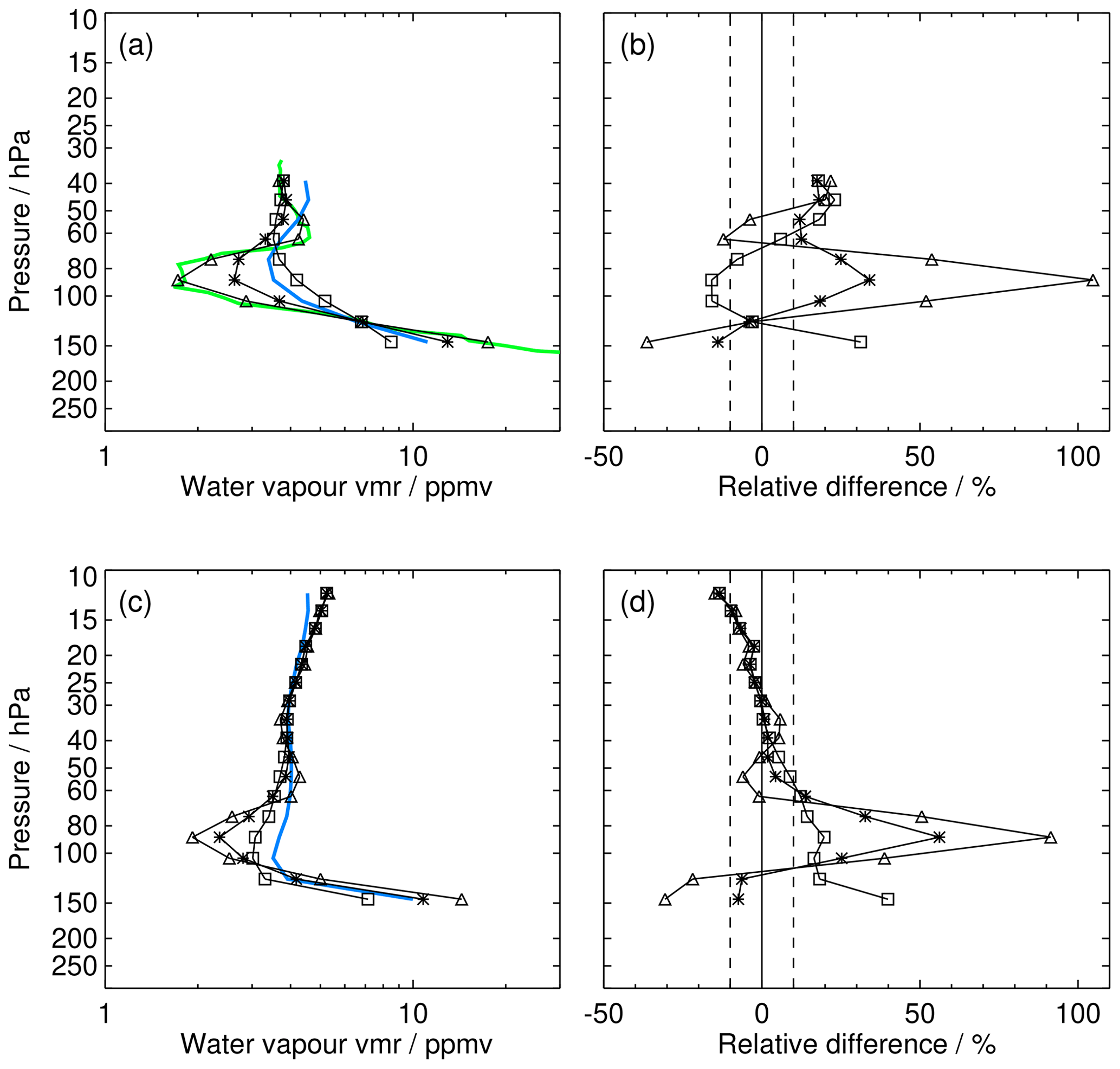
Figure 3Impact of the different methods for adjustment of the vertical grid and resolution of FP profiles (here: BIK) to those of the satellite data records (here: MIR). (a) Sample single profiles of satellite (blue) and collocated FP data (green). Black diamonds denote FP profile directly interpolated onto the coarse common grid; black triangles denote FP profile smoothed with a Gaussian kernel (for details, see the text); black squares denote proper averaging kernels and a priori information applied to FP profile. (b) Corresponding relative differences for the three variants in terms of satellite profile minus FP profile. (c) Averaged profiles for coincident MIR (blue) and FP data at BIK (black, symbols as for data shown in panels a and b). (d) Corresponding relative differences of averaged profiles for the three variants in terms of satellite profile minus FP profile, divided by FP profile.
3.1 Method of calculation of bias and standard error of the mean bias
We assess the bias between satellite data and the FP measurements as the mean difference between the satellite profiles and the coincident transformed FP profiles. For profile data of a given satellite instrument, there is a set of Js FP locations/stations with coincident profiles. At station j the bias for each grid point i is
That is, it does not matter whether the individual differences are calculated first and then are averaged or whether the differences of the appropriate averages are calculated. The bias bj,i is calculated independently for each grid point i and FP station j∈{1…Js} from the available Nj,i coincident observations. For given j, Nj,i can be different for different altitudes because the altitude coverage of a measurement system under assessment may vary from profile measurement to profile measurement. The standard error of the mean (SE) of the bias, which is also the bias-corrected root mean square (rms) difference of the profiles, is calculated as
We consider the bias bj,i as statistically significant if the interval does not include zero.
The mean relative bias (in percent) or percentage bias is calculated by dividing the mean bias bj,i by the mean of the involved FP measurements and multiplying by 100. In all of the following figures, the differences provided are satellite profiles minus FP data. The latter was adapted to the vertical resolution of the satellite data according to Sect. 2.3 and Table 2 and, as well as the satellite data, brought to a common coarser vertical grid.
For a given satellite data set the mean bias over all stations and for a specific altitude range (e.g. 10–30 hPa, 30–100 hPa, and 100 hPa–tropopause as presented in Sect. 3.5) is calculated as follows:
Here Ij represents the set of indices for all the altitudes from the given altitude range and FP comparison data set. The weights wj,i are calculated from the SE of the bias and the ratio of the width Δzj,i of the common coarse grid to the vertical resolution of the satellite measurement, according to
The factor in the weight is used to compensate for the discrepancy between actual vertical resolution and grid width. Without this factor, the SE of the mean bias would directly depend on the grid width via the number of data points which are available in a given altitude range.
Finally the SE of this mean bias over an altitude range is given by
Again, the mean relative bias (in percent) or percentage bias is calculated by dividing the mean bias b by the mean of the involved FP measurements and multiplying by 100.
3.2 Individual comparisons between satellite data records and FP stations
In this section we report on bias profiles of the satellite data records against the FP data from all the stations listed in Table 1. When using terms like, for example, “above 100 hPa”, we always refer to altitudes above 100 hPa: “above” always means “higher up in the atmosphere”. The same applies to terms like, for example, “below 30 hPa”; here, altitudes below the 30 hPa level are meant. For the selected collocations within the coincidence criteria, SAT minus FP differences have been averaged for each satellite data record's full period of coincident measurements. The comparisons for the individual SAT records vary considerably with respect to their measurement periods and numbers of coincidences. Some of the FP stations have operated their balloon soundings only during campaigns; others provide long-term measurement series based on soundings conducted at regular intervals, like LDR, SJC, BLD, and LIN. We have not separated the available comparisons into long-term and short-term series, nor have we tried to detect any temporal variation in biases for the comparisons described in this section. Drifts of satellite data sets will be tackled in Sect. 4.
Figure 4 shows, as an example, the comparison of one SAT data set, namely MLS, to one balloon station, namely TMF, to demonstrate the procedure of bias determination. For this figure, every individual collocated FP profile was treated according to Eq. (5), making use of the MLS averaging kernel and a priori data; since MLS data are provided on a fixed pressure grid, further interpolation to a common vertical grid for calculation of the means over all collocations was not necessary. The comparison was limited to the vertical range above the local tropopause, with the tropopause pressure information estimated from the radiosonde temperature profiles accompanying the FP profiles. The mean SAT and FP profiles, calculated from the closest coincident data pairs, are shown in the left panel of Fig. 4, together with the standard deviations of the respective ensembles. In this example, the mean water vapour profile of the satellite data compares well to the sonde data. Even the variability of SAT and FP mixing ratios are similar, indicating that the random uncertainties of the two measurement types are similar. Further, the deviation between the two measurements due to natural variability appears to be relatively small; i.e. the chosen coincidence criteria are stringent enough to avoid unwanted large differences that could result from location and/or time mismatches between the profiles. The mean bias of the two data sets (middle panel of Fig. 4) above 100 hPa is positive or zero, except for the uppermost data point; i.e. MLS on average has a positive bias relative to the FP, which is at maximum +5 %. Below 100 hPa, close to the tropopause it has a sharp peak of −25 %. The standard error of the mean bias is very small at all satellite reporting levels; i.e. the bias assessment is quite accurate throughout the entire profile. The number of comparisons, in this case between ≈ 30 at the upper and lower ends of the profiles and about 350 for the central part of the profiles, is high and provides the good accuracy of the bias determination. Similar figures for other SAT–FP pairings are provided in the Supplement to this paper.
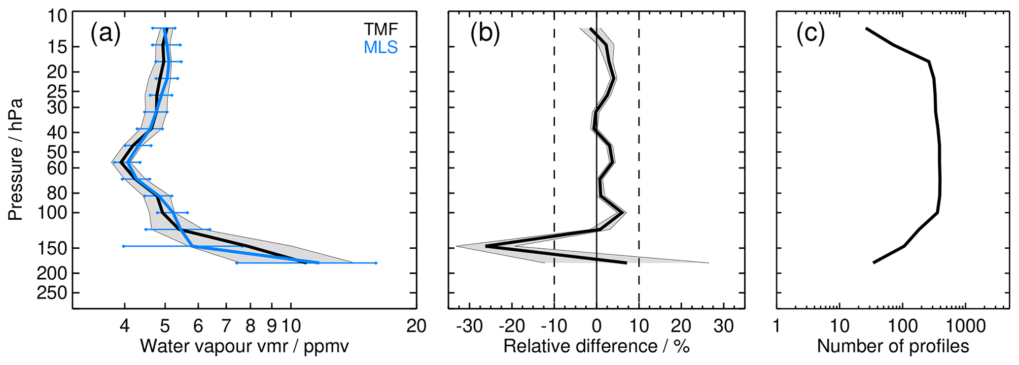
Figure 4Comparison of MLS water vapour profiles with FP profiles at TMF; mean profiles over all coincidences are shown. The individual profiles were cut at the respective tropopause before averaging. (a) Mean profiles (TMF: black, MLS: blue) and their standard deviations (grey shading for TMF and horizontal blue lines for MLS). (b) Relative mean bias and twice its standard error of the mean (grey shading, 2σbias), calculated as the mean differences SAT–FP divided by the mean FP profile and multiplied by 100; the vertical dashed lines enclose the ± 10 % range. (c) Number of data points along the vertical grid. This number can vary over the vertical range, depending on the altitude coverage of the individual coincident SAT and FP profiles, respectively.
3.3 Mean biases of the satellite data records by FP stations
In the following, the comparison of all available satellite data records to one specific FP station is discussed. This comparison provides some insight into potential latitudinal dependencies of the satellite data records' biases. Peculiarities specific to certain FP stations may also show up.
As an example for the comparison of all satellite data to one specific balloon sonde station, Fig. 5 presents the mean relative differences of all available satellite data records to the FP station at BLD (40∘ N). All satellite records having collocations with BLD balloon soundings are shown in this comparison. The presentation is similar to the middle panel of Fig. 4 but for multiple satellites. For the colour coding we refer to Fig. 2. The biases of the SAT data records are shown in two panels in order not to overload the figures. We follow Nedoluha et al. (2017) and separate the data sets in non-MIPAS and MIPAS satellite data.
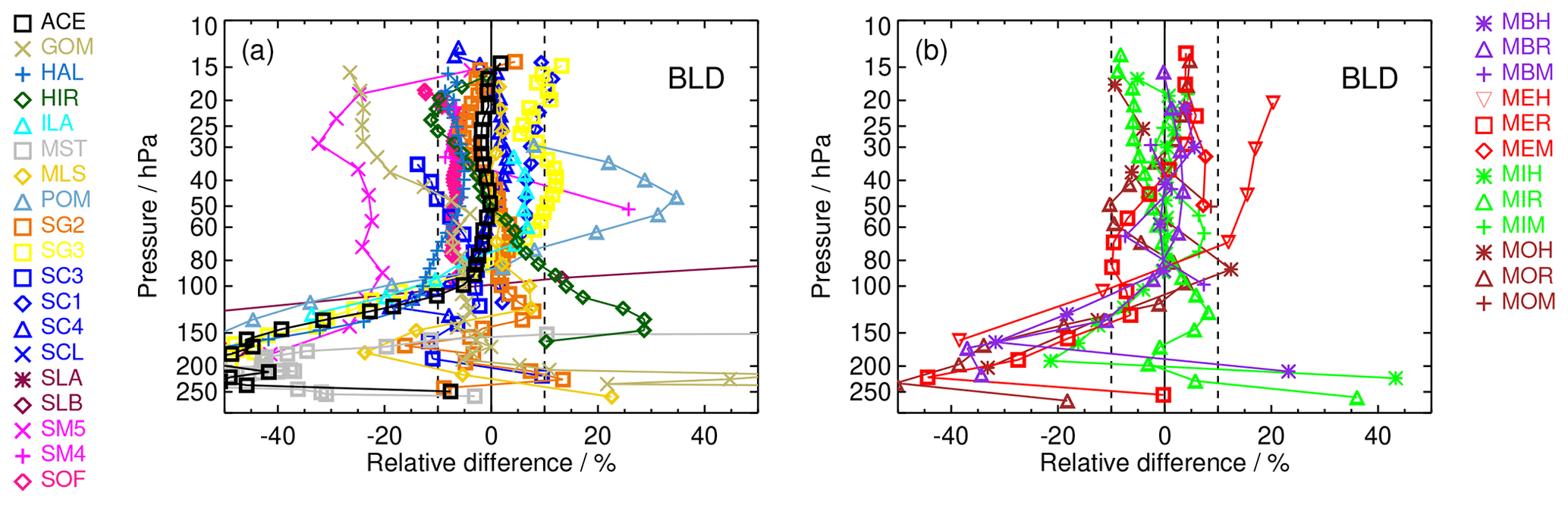
Figure 5Mean relative differences between satellite and BLD FP profiles (40∘ N). (a) All data records except MIPAS. (b) All MIPAS data records. Details of colour coding and symbols for the satellite records are provided in Fig. 2 and Table 2. The profiles were cut at the respective local tropopause before averaging.
We find that, for most of the satellite data records, the bias with respect to the BLD FP data is less than 10 % in the stratosphere between 100 hPa and the upper end of the FP soundings around 10 hPa. Between 100 hPa and the respective tropopause (i.e. the lower end of the profiles), the differences for some SATs become far larger and for many tend to be negative. This is a typical behaviour that can be observed for many stations, mainly in the midlatitudes and high latitudes (see Appendix Figs. A4–A10). In the tropics, however, such a systematic behaviour of the biases is not obvious. Maybe this is because the profiles cut at the local tropopause for tropical sites scarcely reach below 100 hPa (again, see figures in Appendix A2). It is currently unclear what causes these large deviations at the extratropical FP sites.
In case of the comparison to BLD soundings, we identify some large biases that more consistently exceed ± 10 % in the stratosphere above 100 hPa. These are SM5 and GOM, which both show negative biases, and POM and MEH, showing positive biases. All other satellite data sets are largely within 10 % relative difference to the BLD FP data above 100 hPa.
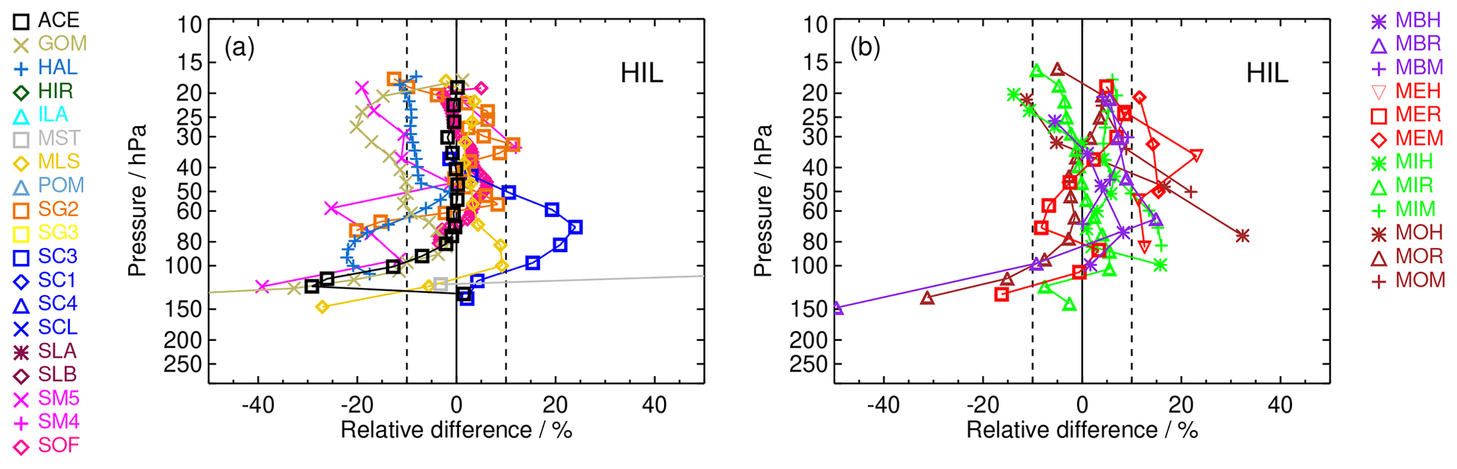
Figure 6 presents an example for HIL (20∘ N), a subtropical Northern Hemisphere station. Generally, we observe some of the same characteristics as for BLD. Due to the higher tropopauses at the lower-latitude sites, the profiles contain few data at pressures >100 hPa. Nevertheless, the negative deviations from the FP data again become larger at the lower end of the profiles. SM5, GOM, HAL, SG2, SC3, MBR, MEH, MEM, MIH, MIM, MOH, and MOM exhibit biases larger than 10 % at multiple altitudes. The biases of the MIPAS data are mostly positive above 100 hPa.
The SAT data records that have large and repetitive biases identified in the BLD and HIL comparisons have larger deviations in most, if not all, FP stations, too. However, the comparisons to many FP stations having a smaller number of coincidences with SAT data due to shorter and/or less dense measurement records have a large spread (not shown in the figures), and the bias determination is less accurate. In general, we can state that the satellite data records that perform well (i.e. virtually all biases <10 %) do so with FP stations having both a large and small number of collocations. These are, in alphabetical order, ACE, HAL (except for the well-known 10 % bias over the entire profile above 100 hPa, Randel et al., 2006; Scherer et al., 2008), MIPAS ESA and IMK/IAA, MLS, SG2, SG3, SC1, SC4, and SOFIE (see Figs. A1–A3).
3.4 Mean biases of the satellite data by data record
Comparison of one satellite data set to several balloon sounding stations provides some insight on how the agreement between SAT and FP may be dependent on latitude. Figure 7 provides, as an example, the comparison of HIR data to all FP stations for which coincident measurements were available (discussion, see below). Similar figures for all satellite data sets are presented in the Appendix (Figs. A1–A3). In the following, we discuss the typical bias behaviour for all these satellite data sets.
ACE-FTS v3.5 (ACE)
ACE (Fig. A1) is in the ± 10 % range for most of the stations above 100 hPa. Larger negative deviations in this altitude range are found in the lower stratosphere for the southeast Asian stations LSA and KMG. At the upper end of the bias profiles, deviations are negative and the satellite data deviate by more than −10 % from stations BEL and TMF. The overall impression is that the ACE biases follow a bent curve with slight negative deviations at the upper end and stronger negative deviations at the lower end of the profiles, showing excellent agreement with the frost point hygrometer profiles between approximately 20 and 80 hPa. For stations in the middle to high latitudes of the Northern Hemisphere, where ACE has its densest sampling, the agreement with frost point hygrometer data is, with deviations within ± 5 %, excellent (e.g. LIN, SOD). The uncertainties of the mean biases (in terms of twice the standard error of the mean, 2⋅SE, 2σbias) are very small in the stratosphere between 100 and 30 hPa, leading to significant biases, at least in the middle to high latitudes, with the exception of BLD where the biases are small and insignificant. In the low latitudes, the uncertainties of the biases are larger, leading to insignificant biases between 60 and 30 hPa.
GOMOS (GOM)
Deviations from frost point hygrometer data for GOM (Fig. A1) vary strongly and cover, except for the comparison to the HAN and the LDR stations, the whole range between −40 % and 0 %. Above 100 hPa the biases have a tendency to be on the negative side and to show increasingly larger negative values with increasing altitude. The comparison to the station data of LDR and HAN contains significant outliers within this comparison, with large positive biases. The biases are all significant at the 2σbias level, except for a few single points where the bias profiles show zero-crossings. The large spread between the stations indicates a significant latitude dependence of the GOMOS data, which might be due to the different stars used as occultation light sources during measurement.
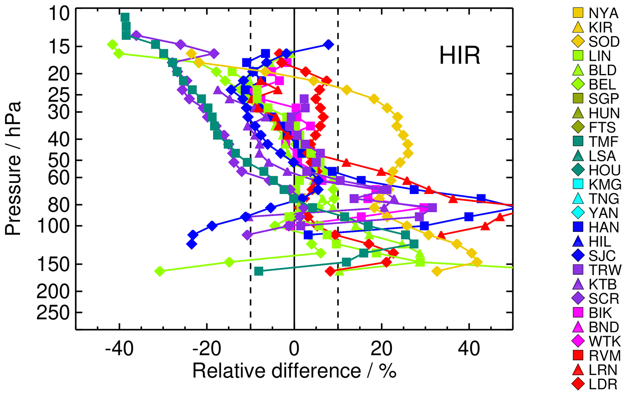
Figure 7Mean relative differences between all the FP stations and the HIR satellite data record. The frost point hygrometer data were adjusted to the vertical grid and resolution of HIRDLS by a smoothing kernel, and the profiles were cut at the tropopause before averaging. Details of colour coding and symbols for the FPs are provided in Fig. 1 and Table 1.
HALOE (HAL)
For HALOE v19 data (Fig. A1), the well-known negative bias of the order of −10 %, seen in measurements after 2001 (Randel et al., 2006; Scherer et al., 2008) over large parts of the stratosphere, is confirmed by the comparisons presented here. Except for some altitudes, at HUN, KIR, SOD, and SGP the deviations from the frost point hygrometers always stay on the negative side, with smallest deviations between −5 % and −10 % in the 20 to 60 hPa range and larger deviations of up to −30 % above and below. The biases are almost all significant; the only exceptions are rare zero-crossings of the bias profiles, for example, for comparisons to the KIR station data. The compactness of the biases of all the stations indicates that HALOE data have a very similar performance over all covered latitudes and related atmospheric conditions.
HIRDLS (HIR)
For most of the stations – with the exceptions of LDR and SOD – the comparison demonstrates a general positive to negative tilt in the bias with increasing altitude for HIR (Fig. A2): Obviously the HIR observations have a positive bias of the order of between 0 to 40 % near 100 hPa and end with a similarly strong negative bias around 10 hPa. The difference with respect to the LDR balloon soundings is more or less constant between 0 % and +10 % above 100 hPa, while the difference to SOD is roughly constant at about +25 % up to 30 hPa and decreases to −20 % from 30 hPa to the upper end of the profile. Below 100 hPa, the biases show a wide spread with some focus around +20 %. The collection of mean difference profiles confirms that the tilted bias, from >20 % near the tropopause to % around 10 hPa, is a distinct property of the HIRDLS water vapour observations. The 2σbias uncertainties of the biases are small, which makes the biases significant everywhere except near the zero-crossings of the bias profiles.
ILAS-II (ILA)
ILA (Fig. A1) could be compared to three stations only; the agreement above 100 hPa is within ± 10 % for BLD and SOD, while ILAS-II deviates from the frost point hygrometer soundings at NYA by −30 % to −40 %. Below 100 hPa, the deviations cover the range between % and +30 %. The biases are all significant except near the zero-crossings of the bias profiles.
MAESTRO (MST)
MAESTRO (Fig. A1) has very few measurements of water vapour above the tropopause. The bias profiles mostly change from −40 % at about 200 hPa to +40 % around 90 to 100 hPa, with large uncertainties, but nevertheless significant deviations. Since we are at the upper limit of MAESTRO's measurement range, we refer to a more appropriate comparison that is provided in a companion paper dealing with upper-tropospheric humidity (Read et al., 2022).
MIPAS (MBR, MER, MIR, MOR)
For MIPAS, all observation modes and data versions from the four processors are shown in Fig. A3. Above 70 hPa, the comparison to the frost point hygrometer data for the NOM RR modes remains within ± 10 % for most cases. The MOR data set is the most compact one, with biases for most stations between +10 % and −10 % for the altitude range of 80 to 20 hPa. Above 20 hPa, a tendency to larger negative biases exists, while below 80 hPa, the profiles develop an increasingly negative bias. The MOH data set is less compact, and it shows a pronounced high bias in the range of 70 to 100 hPa. The MOM data set has a bias >10 % at the lower end of the profiles and a smaller, almost zero bias at the upper end of the profiles. The MIR bias is also quite compact; however it has a rather pronounced tilt from positive values around +20 % near the tropopause to −10 % to −20 % above 30 hPa. Again, for MIH the biases to the various FP sites are less compact but follow in general the characteristics of the MIR data set. The biases for the MIM data set show S-shaped profiles with positive biases % at the lower and much smaller positive biases at the upper end, similar to MOM. For MER and MBR, the biases with respect to the frost point hygrometer stations have a somewhat larger scatter than that of MOR and MIR. Most of their biases remain within ± 10 %; however, some prominent outliers below 60 hPa and above 20 hPa exist.
MBR biases for the northern middle and high latitudes have mostly small uncertainties and are significant except near the zero-crossings of the bias profiles. In contrast, the number of comparisons for the low latitudes is lower; therefore the bias uncertainties are higher, leading very often to insignificant biases. For the LDR FP site (the only in the southern midlatitudes to high latitudes), the biases above 100 hPa are small, and despite small uncertainties, they are insignificant. MER and MOR behave similar to MBR for all FP sites except LDR; deviations from the LDR FP measurements are larger than for MBR, and they are significant over the full altitude range of the profiles. MIR biases are more often significant (although small) than for the other MIPAS data sets. In particular, in the tropics where the biases of the other MIPAS data sets often have higher uncertainties, the MIR biases are significant except for the region of the zero crossings of the profiles. The bias profile with respect to the LDR station is significant except in the troposphere below 200 hPa and at its zero-crossing. The biases for MIPAS HR and MA observations have, in general, larger uncertainties, mainly due to the smaller number of coincidences, and are therefore more often insignificant. Very often, the biases are below ± 10 %, and the uncertainties are larger than that. Consistently significant biases can be found, in general, for larger biases. This is the case for MBH in the comparisons with northern high and midlatitude stations, larger parts of the MEH profiles in all latitudes, and for all MIH and MIM biases that are larger than 2 % or 3 % (absolute). MBM biases are mostly not significant, while MEM biases mostly are. MOH and MOM behave very much like MEH and MEM in terms of significance of their biases.
MLS (MLS)
MLS (Fig. A2) reveals a very compact set of biases that are almost all in the ± 10 % range from 70 to 10 hPa. Exceptions are the comparisons to stations of the Maritime Continent, i.e. BIK, BND, TRW, KTB, and RVM. For these stations, MLS shows a high bias up to +30 % in the altitude range of 100 to 70 hPa. Below 100 hPa, MLS tends to develop a low bias with a peak at −25 % around 200 hPa and a better consistency to frost point hygrometer data, again in the ± 10 % range, close to the local tropopause. In the northern high and midlatitudes, the uncertainties of the biases are extremely small, leading to significant but small (mostly +5 % to 10 %) deviations from the FP data in the stratosphere above 100 hPa. Even in the low latitudes, the uncertainties are small enough to make most of the deviations significant, in particular the deviations from FP stations on the Maritime Continent. The bias with respect to the LDR FP site is below 5 % above 70 hPa and significant, due to the extremely small uncertainty. The larger biases below 100 hPa are mostly significant, too.
POAM-III (POM)
POM3, as an instrument covering the northern high latitudes only, has coincidences with the most northern stations NYA, SOD, KIR, and BLD (Fig. A1). The biases to the three former stations are rather small, providing curved bias profiles with negative values around −20 % below 100 hPa and above 20 hPa and positive values of up to +20 % between 100 and 40 hPa. The comparison with the sonde data of BLD gives a somewhat different picture: here the biases increase from extreme negative values beyond −40 % below 100 hPa to +35 % around 50 hPa and remain in the 10 % to 35 % range above. The hygropause in the POM3 profiles near BLD, i.e. the altitude with lowest water vapour VMR, is much lower than in the frost point hygrometer data, and the mean profile below the hygropause is displaced towards lower altitudes, which both contribute to the increasingly larger negative bias below 100 hPa. All biases are significant except near the zero-crossings.
SAGE-II (SG2)
SG2, as another instrument besides HALOE, providing water vapour observations for decades, has been used a lot for construction of longer-term global water vapour data time series. The comparisons to frost point hygrometer station data (Fig. A1) provide some scatter; however most data points lie within ± 20 % deviation and a larger part also within ± 10 %. The comparisons to SOD form an exception with positive deviations of approximately 25 % over a larger part of the stratosphere (90 to 35 hPa). The number of coincidences, however, is very small (around 10) for this FP site. The uncertainties of the bias profiles are often of the order of ± 5 %, which makes some deviations in the northern high and midlatitudes insignificant. The bias with respect to BLD FP observations, however, is significant in the stratosphere above 100 hPa despite the deviations being less than 5 % over a large part of the profile. The same is true, although to a smaller part of the profile, for the comparison to the LDR FP site (the altitude near the zero-crossings of the profiles always excluded). For the low-latitude FP sites, a general comment is difficult to make because of strongly oscillating bias profiles and sometime considerable uncertainties. Nevertheless, also in this latitude region significant biases can be found despite larger uncertainties.
SAGE-III (SG3)
SG3 data (Fig. A1) could be compared to the northernmost stations (NYA, KIR, and SOD), BLD, and LDR only. The comparisons agree well, indicating a bias within the ± 10 % range, with two outliers of the order of +20 % at about 70 and 15 hPa. The comparison to the BLD balloon data indicates, similar to POM3, a hygropause that is lying too low and displacement towards lower altitudes of the profile part below as the reason for the increasingly large negative bias below 80 hPa. Uncertainties of the biases are small enough to make the biases significant over the full altitude range, except near the zero-crossings.
SCIAMACHY (SC3, SC1, SC4, SCL)
The SC3 observations (Fig. A2) cover the altitude range from the tropopause up to approx. 30 hPa. Above 100 hPa, the comparisons to the FP stations provide a large scatter from −40 to more than +50 %. The stations on the Maritime Continent and in the Indian Ocean (pink, purple, and partly red colours) seem to provide the highest positive biases, while for northern midlatitude stations the biases tend to be in the ± 10 % range and rather on the negative side. Near to the upper end of the SCIAMACHY profiles, around 30 hPa, the deviations to the sonde station data converge to a bias range of −20 % to +5 %, with only two outliers, and most of the biases within the ± 10 % range. The biases with respect to the BLD FP site are significant below 150 hPa and above 70 hPa. Other sites for which the biases turn out to be significant, at least over a large part of the profiles, are SOD, LIN, and SGP, all revealing negative biases. Biases for HIL, SJC, TRW, BIK, RVM, and LRN are significant for at least a part of the profile and positive, while the comparison to LDR shows insignificant and rather small biases. The SC1 and SC4 data sets, both solar occultation observations, have in common that only stations from moderate to high northern latitudes contribute to the comparisons (Fig. A1). The SC1 relative biases are within ± 10 % between 100 and 20 hPa, and above and directly below this altitude range they tend towards more negative values. Biases and uncertainties are rather small and of the same order of magnitude for KIR and NYA. Therefore the biases are largely insignificant. The other stations reveal significant biases. SC4 shows biases within ± 10 % between 100 and 20 hPa for four out of six FP sites. Biases with respect to NYA and KIR, however, are at about 10 % at 100 hPa but decrease to about −20 % at 30 hPa. All biases except near the zero-crossings of the bias profiles are significant. The SCIAMACHY lunar occultation data set has coincidences with the FP station of LDR only (Fig. A1). The bias for this site is between 10 % and 20 % and significant at all altitudes.
SMILES (SLA, SLB)
The comparison of SMILES water vapour observations from their channel A and B (Fig. A2) to frost point hygrometer sonde data shows a large scatter and prominent biases reaching from −40 % and more below 100 hPa to +40 % and more between 40 and 30 hPa. Due to the short mission lifetime of SMILES, the number of coincidences with frost point hygrometer soundings is, however, very limited. As a consequence, uncertainties of biases are rather large. Nevertheless, the biases are significant except near the zero-crossings of the profiles.
SMR (SM5, SM4)
SMR 544 GHz comparisons with frost point hygrometer data reveal a large scatter of the biases over ± 40 % and more (Fig. A2). Most of the bias profiles are negative, and there seems to be a certain concentration of biases around −30 %. There is no latitude dependence obvious. Despite the long lifetime of the SMR mission (which is still operational at the time of this writing) and its rather dense global coverage, the number of coincidences range between 10 and 100 for most of the stations only. The spread of the coincident SM5 profiles is, however, far larger than the spread of the frost point hygrometer profiles, indicating that the SM5 profiles have a considerable measurement error (see Fig. S29 in the Supplement). The SMR 489 GHz observations of water vapour are available above 50–60 hPa only. They are more compact than the 544 GHz observations, with biases between −20 % and +20 % and most data points falling into the ± 10 % range. However, for this observation channel, a much smaller number of stations providing coincident balloon soundings are available, and the number of coincidences per station is often below 10. Therefore, the biases have often large uncertainties. Nevertheless, most of the biases are significant.
SOFIE (SOF)
For SOFIE, comparisons with frost point hygrometer data from SOD, BLD, LIN, HIL, SJC, and LDR are available (Fig. A1). The comparisons to all frost point hygrometer data are very compact. Above 100 hPa, almost all data points of the biases fall into the ± 10 % range, and many of them are even closer than ± 5 % to the frost point hygrometer data. The uncertainties are small, making even the tiny deviations from FP measurements at BLD or LDR significant.
3.5 Synopsis of the bias assessment
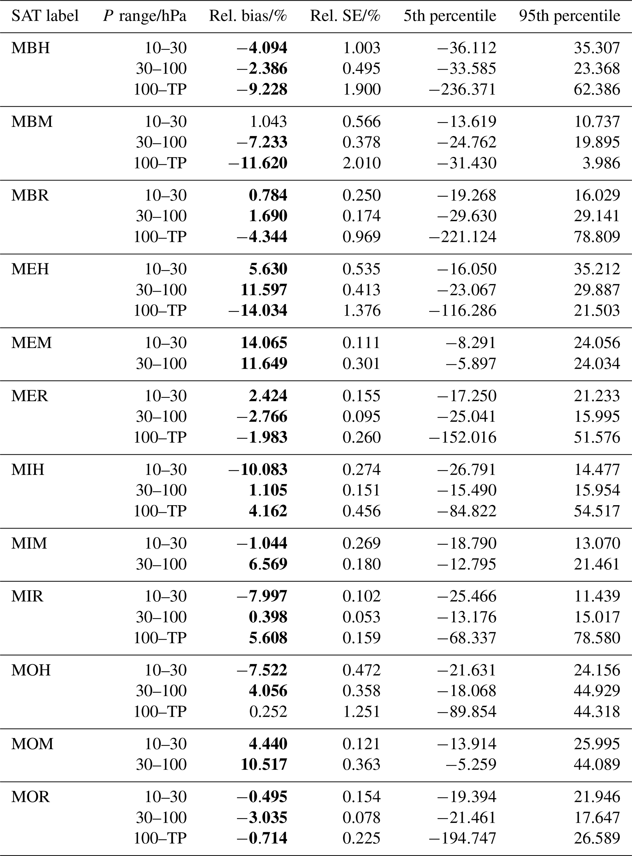
For the overall assessment of biases of SAT records against FP profiles, we have averaged the results from all stations in each of the following three pressure ranges: tropopause to 100 hPa, 100 to 30 hPa, and 30 to 10 hPa. The average biases and their standard errors were calculated with Eqs. (9) and (11), respectively. They are listed in Tables 3 and 4. In Fig. 8 thick horizontal bars show average biases plus/minus twice the respective standard errors to indicate the 95 % confidence limits. Additionally, the 5th and 95th percentile values are marked in the plots and listed in the tables.
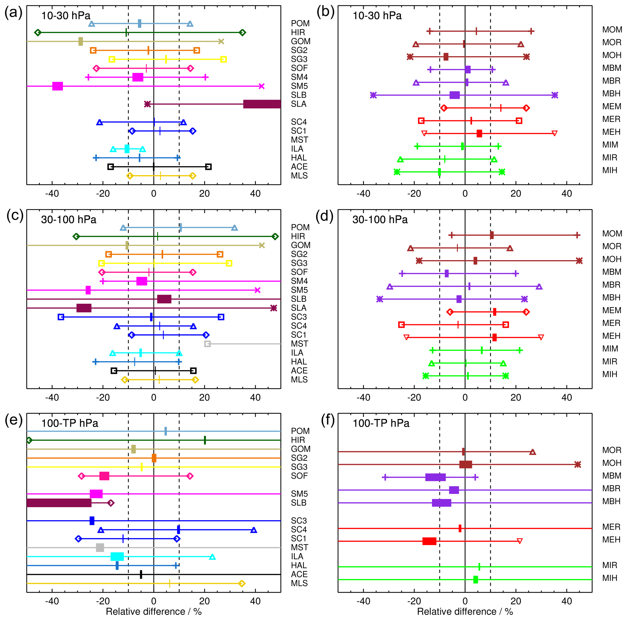
Figure 8Relative differences of satellite and FP data averaged over all sites and the three pressure ranges 10–30 hPa (a and b), 30–100 hPa (c and d), and 100 hPa to tropopause (e and f). The panels on the left show comparisons for all satellite instruments except MIPAS. In the right column all MIPAS comparisons are displayed. For colour coding and symbols see Fig. 2. Thin lines between symbols span the 5 %–95 % range of the data, while thick bars indicate the range of twice the standard errors (2×SE) around the mean biases. The actual average bias values are given by the centre of the thick bars. For the 10–30 hPa panel, SLB and MST biases and the 5 %–95 % range of data are completely beyond the relative difference scale (see Table 3 for the actual values).
Table 3Tabulated data used in the left columns of Fig. 8 for the non-MIPAS data sets; 100–TP means the pressure range from 100 hPa down to the tropopause. Statistically significant biases are presented in boldface text. Note that the column “Rel. SE” does not give the relative value for 2×SE used for the plots in Fig. 8, but only the relative value for the SE.
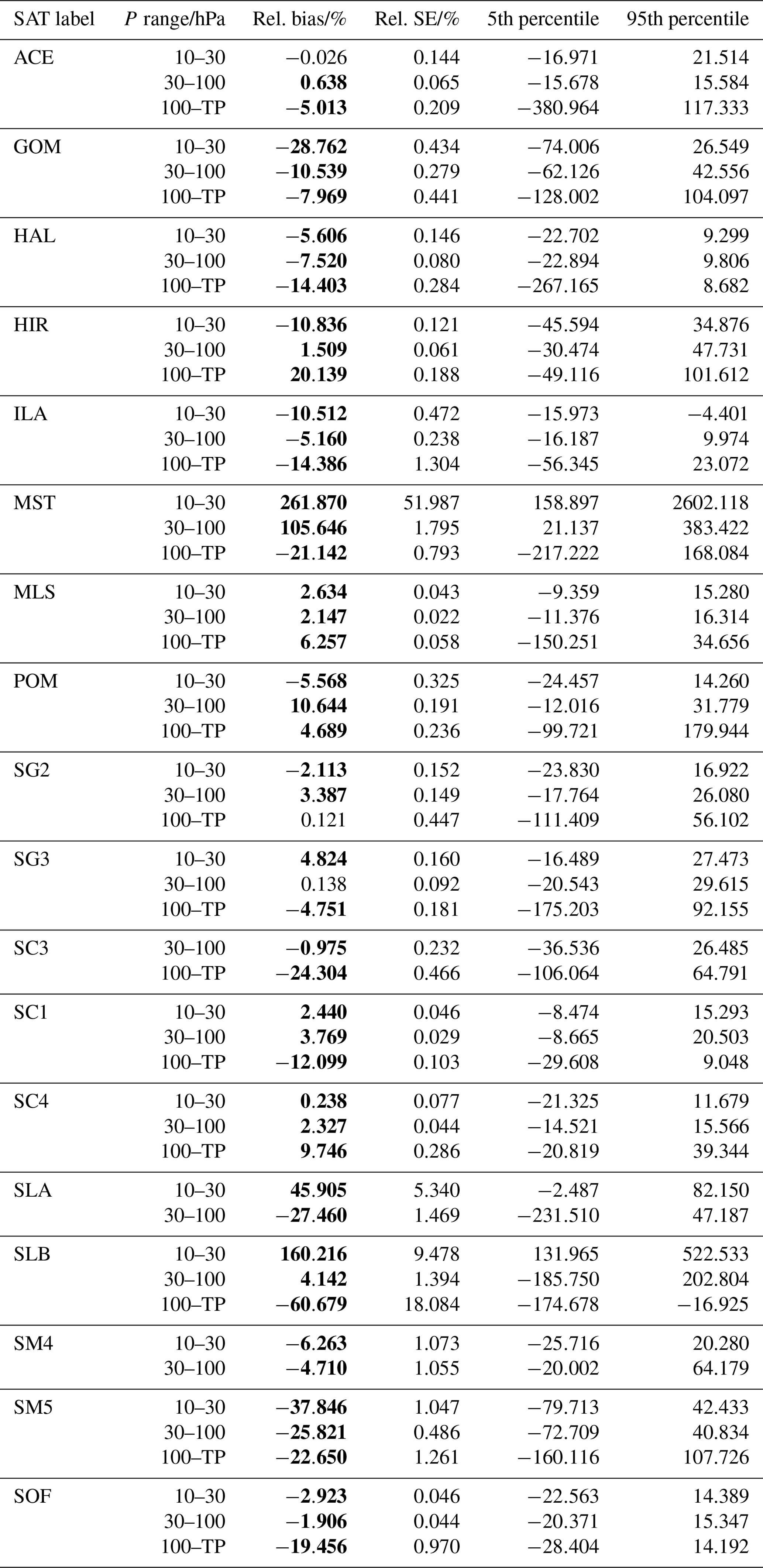
Table 4Tabulated data used in the right columns of Fig. 8 for the diverse MIPAS data sets; 100–TP means the pressure range from 100 hPa down to the tropopause. Statistically significant biases are presented in boldface text. Note that the column “Rel. SE” does not give the relative value for 2×SE used for the plots in Fig. 8, but only the relative value for the SE.
In the 10–30 hPa altitude range, most of the satellite data records have mean biases within the ± 10 % range, and some of them show even better overall agreement with the FP data. ACE, MLS, SG2, SG3, SC1, SC4, and SOF have very accurately determined biases of smaller than ± 5 %. Data records with mean biases larger than ± 5 % but less than ± 10 % are HAL, POM, and SM4. For all three, the bias accuracy is very good. Data records with biases larger than ±10 % are ILA, MST, SLA, SLB, SM5, GOM, and HIR. Except for MEM and MIH , the MIPAS data records are all within the ± 10 % range regarding their bias in the 10 to 30 hPa altitude range with the majority of these being within the ± 5 % range. The three ESA data products have all a positive bias, while the three IMK/IAA data records have all a negative bias. Except for the ESA product, water vapour derived from the MIPAS middle atmosphere measurement mode shows agreement with FP data of better than 5 %.
In the altitude range of 30–100 hPa, HIR, SG2, SG3, SOF, SM4, SLB, SC3, SC4, SC1, ACE, and MLS have biases less than ± 5 %. However, SM4 and SLB have very large uncertainties of the biases. HAL and ILA have biases less than ± 10 %. POM and GOM have biases just greater than 10 % in the 30 to 100 hPa altitude range, while the biases of SM5, SLA, and MST far exceed 10 %. Except for MOM, MEM, and MEH, MIPAS data sets fall into the ± 10 % bias range. MOR, MOH, MBR, MBH, MER, MIR, and MIH show even biases lower than ± 5 %.
In the tropopause to 100 hPa altitude range, the biases, and especially the data spread, become large for many of the SATs. Data records with biases below ± 10 % are POM, GOM, SG2, SG3, SC4, ACE, and MLS. Of these, POM, SG2, and SG3 show biases below ± 5 %. ACE just misses this value. For the MIPAS data sets, MOR, MOH, MBR, MBH, MER, MIR, and MIH are within ± 10 % bias. MOR, MOH, MBR, MER, and MIH even stay within the ± 5 % range. For all data records, the uncertainties of the biases increase compared to the other altitude ranges.
Linear temporal trends in the relative differences between stratospheric water vapour mixing ratios reported for satellite (SAT) and frost point hygrometer (FP) measurements are hereinafter referred to as “drifts”, expressed in units of % yr−1. Relative differences in SAT and FP mixing ratios (100 % × (SAT–FP)/FP) were calculated using FP mixing ratios as the divisors. As the bias analyses above, this investigation of drifts is based on FP and satellite-based profile measurements that are coincident in space and time according to the criteria provided in Sect. 2.2. Also analogous to the bias evaluations, before comparing to SAT profiles, the vertical resolution of each FP profile was degraded to that of the corresponding satellite's reporting levels and placed on its grid of reporting pressures (i.e. convolved) using satellite-specific averaging kernels or more generic Gaussian-shaped smoothing kernels (see Sect. 2.3 and Table 2). To minimize the influences of tropospheric air on this evaluation of stratospheric measurements, the reporting levels of SATs were limited to those above the local tropopause (Sect. 2.2). Similar analyses of biases and drifts between SAT and FP measurements of tropospheric water vapour have already been published by Read et al. (2022).
Several of the methods employed here to evaluate drifts are slightly different from those used above for the bias analyses. In cases where multiple profiles from a given SAT were identified as coincident with a FP profile (a “coincident cluster”), the median SAT mixing ratio and standard error of the mean SAT mixing ratio were calculated for each cluster, as was done in Hurst et al. (2014). The convolved or smoothed FP mixing ratio profile (see Sect. 2.3) was then subtracted from the median SAT mixing ratio profile. The advantage gained using median mixing ratios instead of averages is that they are much more resistant to skew by statistical outliers. The SAT–FP mixing ratio differences (in ppmv) were divided by the FP mixing ratios and then multiplied by 100 % to produce the SAT–FP relative differences analysed here. For each unique pair of FP sites and satellites, the drift at each SAT reporting level was independently determined using a weighted linear regression fit to the time series of SAT–FP relative differences, with statistical weights based on the standard error of the mean SAT mixing ratio for each coincident cluster.
4.1 Evaluation of data records for drift analysis
Unlike the bias evaluations, an analysis of drift in SAT–FP relative differences requires a sufficient number of differences over an adequately long period of time to detect and determine statistically robust trends. The unique pairs of SATs and FPs evaluated for biases (see Tables 1 and 2) included many with short and/or sparse time series of relative differences. Typically, the statistical uncertainties of drifts determined for these pairs were large, and the calculated drifts were very sensitive to the removal of one data point from the time series. Simple tests of drift uncertainties and sensitivities for time series with varying lengths and data densities were performed. The results revealed that robust drift statistics were consistently produced for time series > 5 years in length and composed of at least one difference in 67 % of the years covered. Of all the unique SAT–FP pairs analysed for biases, only 64 provided difference time series that met these more stringent criteria for drift analysis. This excluded several time series > 5 years in length but with only short-term “bursts” of FP data from intensive measurement campaigns.
Table 1 identifies the seven FP sounding sites that paired with SATs to provide at least one time series of differences that met the record length and data density criteria. Table 2 identifies the 20 SAT retrievals that paired with FP sites to produce at least one qualifying time series. Of these 20 SAT retrievals, 8 were for MIPAS, 3 for SCIAMACHY, 2 for SMR and 1 each for 7 other SATs. In total, 1146 time series of SAT–FP relative differences were analysed for drift at each SAT reporting pressure ranging from 275 to 13.1 hPa. These time series are based on several thousand satellite profiles and just over 900 unique FP profiles over 7 sites.
The numbers of reporting levels for each unique SAT–FP pair that met the drift analysis criteria are presented in Tables 5 and 6. Each SAT–FP pair provided difference time series at an average of 18 reporting levels over an average of 3 FP sites, though the individual coverages ranged widely from 1 to 74 reporting levels and 1 to 7 sites. For example, MIPAS Bologna V5R v2.3 MA (“MBM”) retrievals produced only a single qualifying time series of differences at 43 hPa over the BLD site, while MAESTRO (“MST”) retrievals produced qualifying difference time series at an average of 50 reporting levels over each of 4 FP sites. Since the records for HAL and SG2 extend only 5–6 years into the new millennium, they overlap adequately only with the FP record at BLD. The MLS is the only SAT that paired with all seven FP sites.
4.2 Methods for quantifying drifts
Each time series of SAT–FP differences was examined for statistical outliers by performing a preliminary standard linear regression analysis. Data points with residuals from the fit line that were >2.5 times the mean of the absolute values of the residuals were omitted from further analysis. This method of outlier filtering removed an overall average of 5.7 % of the data points from the time series before they were analysed for drift.
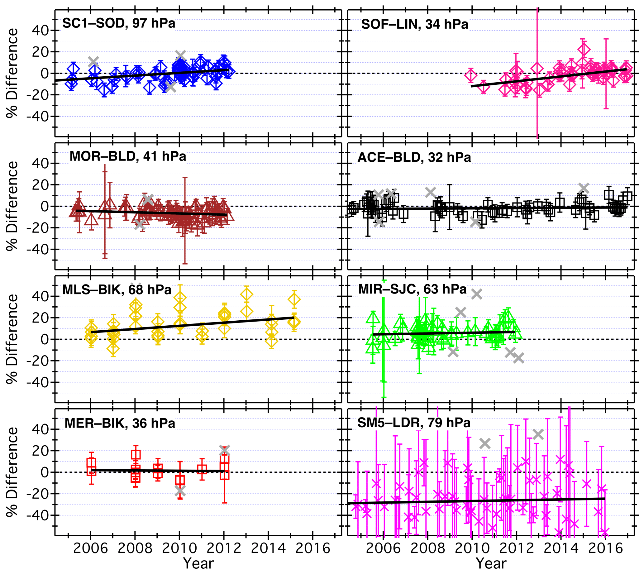
Figure 9Time series of SAT–FP relative differences for eight unique pairs of satellite retrievals and FP sites. See Tables 1 and 2 for the three-letter codes that represent the relevant FP sites and satellite retrievals. The SAT reporting pressure for the time series shown is given in each panel. Vertical error bars depict the uncertainties in SAT–FP differences that factor into the weighted linear regressions used to calculate the black trend lines. Grey crosses are data points identified as outliers and omitted from the analyses.
Drifts in SAT–FP differences were determined using weighted linear regression analyses (Fig. 9). The weight Wi applied to each difference was computed as the squared reciprocal of its uncertainty (Eq. 12). The uncertainty λi of each difference was calculated (in quadrature) from the relative standard error (σi) of the mean mixing ratio of the “coincidence cluster” of satellite profiles (in %) and the ± 6 % uncertainty of stratospheric water vapour measurements by FPs (Hall et al., 2016; Vömel et al., 2016). Each fitting weight was then scaled to the 95 % level of confidence using the Student t value for the number (n−1) of satellite profiles in each coincidence cluster. In this way, differences with smaller uncertainties had greater weights and therefore stronger influences on the linear regression fits.
SAT–FP differences based on only a single coincident satellite profile (a rare occurrence) were assigned the smallest weight calculated for the entire time series. Consequently, these single profile differences had the weakest influence on the linear regression analyses of drift.
The slope of the weighted regression fit line for each time series of relative differences was utilized as the best statistical estimator of the linear temporal drift (% yr−1) in the differences. Similarly, the 95 % confidence limits of calculated slopes were considered the best estimates of drift uncertainty and thus used to evaluate the statistical significance of the drifts. In this analysis, a drift in SAT–FP differences at a given reporting pressure is considered to be statistically significant if the 95 % confidence interval of the regression line slope does not include zero.
The vertical profiles of drifts determined for four unique SAT–FP pairs (Fig. 10) and all SAT–FP pairs (Figs. B1–B5) illustrate how the 95 % confidence intervals determine statistical significance. In these plots, if the 95 % confidence interval (full span of the error bar) does not intersect the vertical line for zero drift, the drift is labelled significant. Red (blue) markers indicate the statistical significance (non-significance) of the drifts at all reporting pressures. Figure 10 also shows that the reporting pressures for some SAT–FP pairs span only very limited ranges (e.g. 100–15 hPa for SOF at LIN), while those for other pairs cover much wider intervals (e.g. 196–18 hPa for MIR at BLD). The ranges of reporting pressures were typically smaller over tropical FP sites because their tropopause cut-offs were at lower pressures than the extratropical sites.
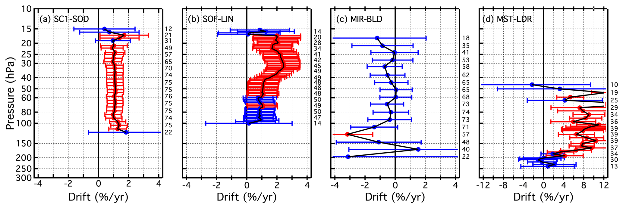
Figure 10Vertical profiles of drifts (filled circles) and their 95 % confidence intervals (horizontal error bars) for four different SAT–FP pairs. Blue error bars denote drifts that are not significantly different from zero, while red error bars indicate statistically significant drifts. Numbers in black text to the right of each panel present the number of SAT–FP differences in the time series analysed for drift at the corresponding pressure levels. Note that the x-axis scale is different for panel (d).
4.2.1 Special case of MLS drifts
The data, trend lines, and correlation coefficients produced by weighted linear regression fits of all 1146 SAT–FP difference time series were visually checked for consistency and quality. The abnormalities most often revealed were the poorer fits (and lower correlation coefficients) associated with MLS–FP differences over most of the FP sites. Visually, many of the MLS–FP time series show little or no evidence of drift until ∼ 2010, after which positive trends in the differences become readily apparent (Fig. 11). These positive, post-2010 drifts in MLS–FP differences were previously reported from similar drift evaluations above the BLD, HIL, LIN, LDR, and SJC sites (Hurst et al., 2016).
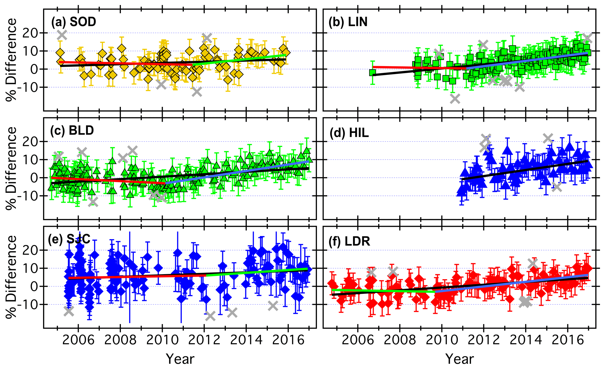
Figure 11Time series of relative MLS–FP differences at 68 hPa over six different FP sites. As in Fig. 9, vertical error bars represent the uncertainties in differences, and grey crosses are data points identified as outliers and omitted from the drift analyses. Black lines depict the trends determined by weighted linear regression fits to the entire records of differences. Coloured lines show the linear trends in two distinct time periods (except at HIL) that are separated by a statistically significant changepoint, as determined by piecewise continuous weighted linear regression fits (see Sect. 4.2.1).
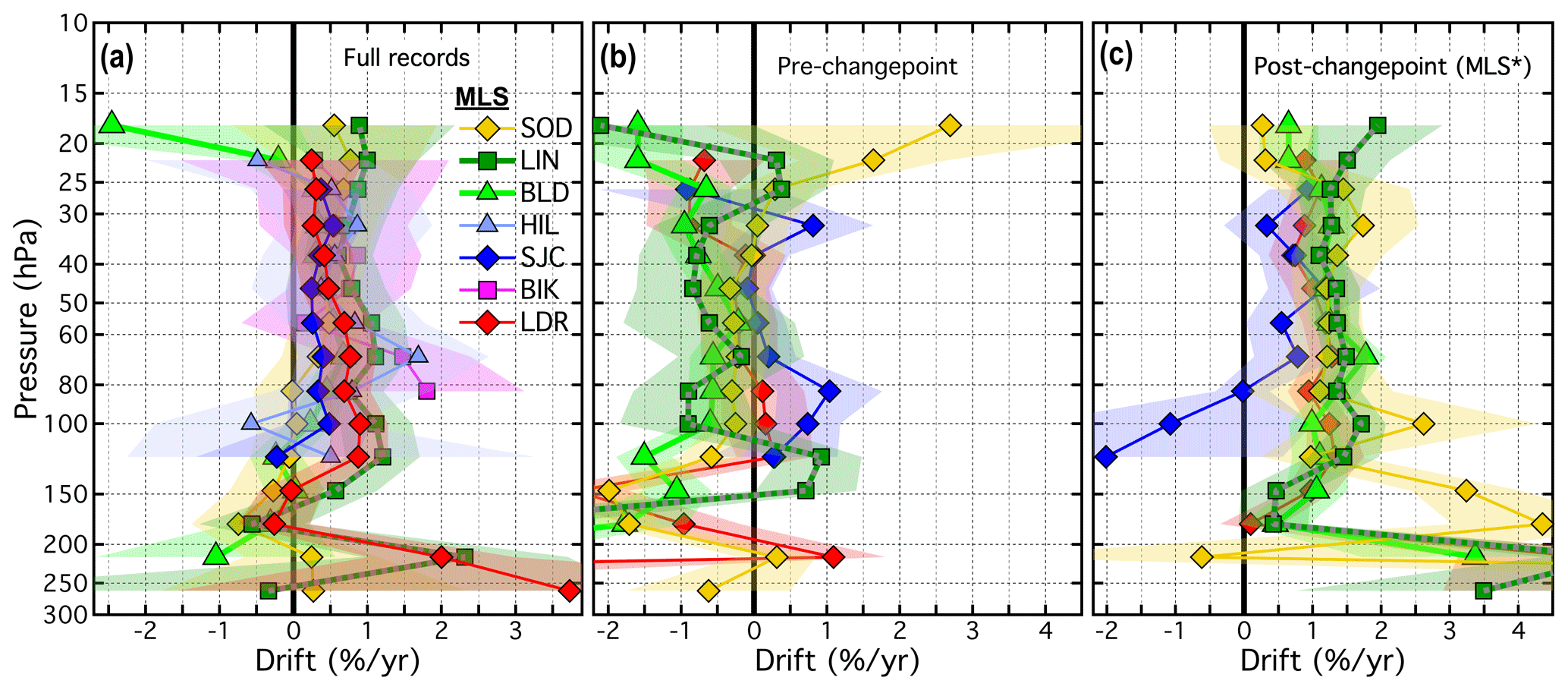
Figure 12Vertical profiles of drifts in (a) MLS–FP differences spanning the entire records (2004–2016), (b) for the 2004 to ≈ 2010 pre-changepoint period, and (c) for the ≈ 2010 through 2016 post-changepoint period (i.e. MLS∗). The legend applies to all three panels, but drifts at HIL and BIK are not available for panels (b) or (c). The coloured-matched shading surrounding each profile represents the 95 % confidential intervals of the drifts over that site.
The alternative methodology used here, analogous to that described by Hurst et al. (2016), is a piecewise continuous weighted linear fitting procedure for each time series of relative MLS–FP differences. The fitting algorithm divides each time series into two distinct periods by identifying the point in a record when a statistically significant change in the trend occurred, the “changepoint” as described by Lund and Reeves (2002). The optimal changepoint is the date for which linear fits before and after it yield the smallest root mean square (rms) of residuals. In the case of MLS–FP differences, the piecewise continuous weighted linear fits substantially improve the “goodness of fit” for each time series (Fig. 11). Compared to the full time series regression fits of MLS–FP differences, the two-piece linear fits decrease the rms of residuals at each of the five FP sites by 1 % to 8 %, with an average reduction of 4 %. For the MLS–BIK time series, no statistically significant changepoints were identified because the FP record at BIK is dominated by data obtained during intensive but short-lived, annual measurement campaigns (Fig. 9). For HIL, the records of MLS–HIL differences lack adequate data before ≈ 2010 for the time series to be analysed by this method (Fig. 11). The piecewise continuous fits were therefore performed only on the MLS–FP time series at SOD, LIN, BLD, SJC, and LDR. The drifts and other statistics reported for the post-changepoint fits to MLS–FP difference time series are denoted by the SAT code MLS∗.
MLS retrievals at 31 of 70 pressure levels (44 %) in the 121–18 hPa range over seven FP sites exhibited full-record drifts that are positive and statistically significant (Fig. 12). When piecewise continuous linear fits were performed on the same MLS–FP differences, excluding those at HIL and BIK, pre-changepoint drifts were positive and statistically significant at 4 of the 52 (8 %) reporting levels (Fig. 12b), while 46 of the 52 (88 %) post-changepoint drifts were significant and positive (Fig. 12c). The vast majority (90 %) of the positive post-changepoint MLS∗ drifts were stronger than the full-record MLS drifts (Fig. 12). For MLS-reported pressures from 68 to 22 hPa over all FP sites except HIL and BIK, post-changepoint drifts were an average of ±σ of 2.4 ± 1.0 times stronger than full-record drifts. Though the piecewise fits better represent the MLS–FP time series and reduce the rms of residuals compared to full-record fits, their uncertainties are larger than for the full-record drifts because the pre- and post-changepoint records have substantially smaller data populations.
4.3 Drift profiles for the unique SAT–FP pairs
The drifts determined for all 21 SATs (MLS∗ included), each paired with 1 to 7 FP sites, are presented as vertical profiles in Fig. 13 and in Figs. B6 and B7. Similarly, Figs. 14 and B8–B9 show the drifts of all paired SATs at each of the seven FP sites. Both sets of figures are analogous to Fig. 10 except each panel of Fig. 13 shows the drifts of a unique SAT over multiple FP sites using the coloured symbol scheme from Fig. 1, while each panel of Fig. 14 shows the drift profiles of multiple SATs over each FP site using the coloured symbol scheme from Fig. 2. In some panels of Figs. 13, B6, and B7, the colours and symbols for some SAT–FP pairs were slightly adjusted to help differentiate between the drift profiles at specific FP sites, for example LIN and BLD. Another modification to Figs. 13, B6, and B7 is that the 95 % confidence intervals are represented by shaded, symmetric envelopes that match the colours of the drift profile markers and connecting lines. For some SATs the drifts were relatively uniform with pressure, while the drifts of others were much more variable. Note that the reporting pressure for some SATs are the same for each FP site, while for other SATs they are not.
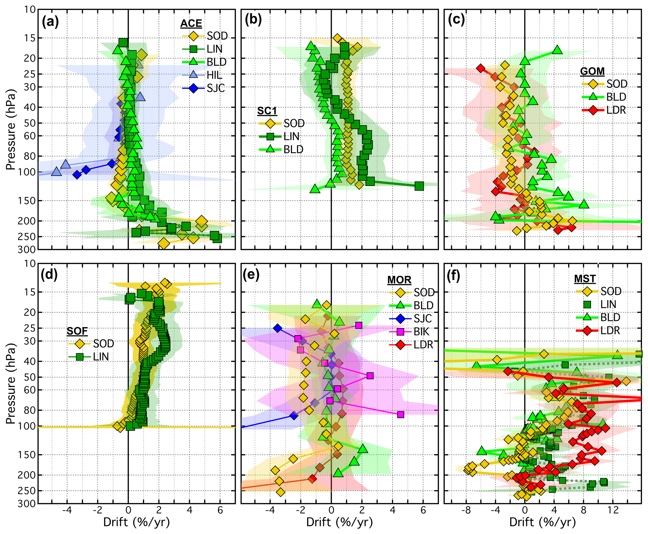
Figure 13Vertical profiles of drifts in SAT–FP differences. Each panel displays the drifts for one SAT paired with 2–5 different FP sites. Drifts over each FP site (connected coloured markers) are presented with their 95 % confidential intervals (coloured-matched shading). Shading that does not cross the black vertical line at 0 % drift indicates drifts that are statistically significant. Note that the x-axis scale for the far right column is expanded to show the drifts with greater clarity.
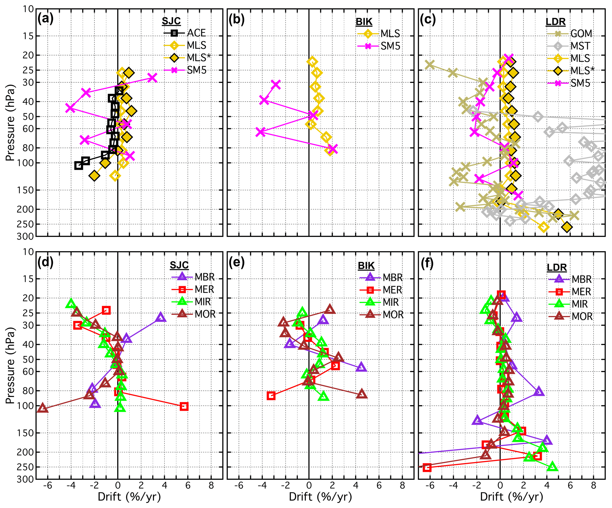
Figure 14Vertical profiles of drifts in SAT–FP differences. Each panel displays the drifts for the multiple SATs paired with each FP site. Profiles for non-MIPAS SATs appear in the top row, and for MIPAS SATs appear in the bottom row. Drifts for each SAT are represented by unique coloured markers according to Fig. 2. MLS∗ refers to drifts in MLS from ∼ 2010 through 2016, as discussed in Sect. 4.2.1.
There is a general tendency for the uncertainties of drifts to broaden at the extremes of the reporting pressure ranges. This often occurred because there were sharp drop-offs in data populations of the difference time series at the highest and lowest pressures and, therefore, fewer data points for the weighted regression fits. Two factors affecting uncertainties at the high and low pressure ends of drift profiles are the annual cycles in extratropical tropopause pressures that reduce the data populations at the highest reporting pressures during summer months and the altitude ceilings of balloon-based FP profiles that limit data populations at the lowest reporting pressures.
Of the 21 different SATs analysed here, some have drift profiles over multiple FP sites that are statistically equivalent when the drift uncertainties are considered. For example, the ACE drift profiles ≤ 85 hPa are statistically the same over all five FP sites (Fig. 13a). Drift profiles for SC1 (Fig. 13b) at LIN and BLD also statistically overlap over their entire pressure ranges, although the drifts ≥ 51 hPa are significant over LIN but not BLD. Drifts for SOF over SOD and LIN (Fig. 13d) also statistically overlap over their entire pressure ranges, with all drifts in the 58–17.2 hPa interval over both sites being positive and significant. Drift profiles for SATs at other FP sites are not always statistically the same, as exemplified by the absence of statistical overlap in SC1 drifts at 10 reporting levels over SOD and BLD in the 45–23 hPa interval (Fig. 13b), MST drifts at 6 reporting levels (170–140 hPa) over SOD and BLD (Fig. 13f), and SC4 drifts at 4 levels (35–25 hPa) over SOD, LIN, and BLD (Fig. B7d).
Given the vertical profiles of drifts in Figs. 12, 13, and 14, plus those provided in the Appendix (Figs. B1–B9), it is evident that a few SATs exhibit statistically significant drifts at many reporting levels over multiple FP sites. Of the 1213 time series of SAT–FP differences analysed here for drift (includes analyses of MLS∗), 419 (35 %) of the drifts were statistically significant. Of the 21 SATs examined here, MLS∗ and SOF had the highest percentages of reporting levels (84 % and 70 %, respectively) with statistically significant drifts over their associated FP sites. The percentages for four other SATs were >40 %: MST (47 %), SC1 (46 %), SC4 (41 %), and MLS (41 %). Overall, these 6 SATs were associated with 339 (81 %) of the 419 statistically significant drifts.
Though the identification of statistically significant drifts is an important result, a more critical metric is the strength of a drift, as this limits the utility of a satellite data set when trying to detect temporal trends in stratospheric water vapour. For this work, a drift of −1 % yr−1 ( ppmv per decade in the middle stratosphere) in a data set would either completely mask a real trend of +0.5 ppmv per decade or double a real trend of −0.5 ppmv per decade, effectively rendering the data set unusable for detecting a trend of this magnitude. With this in mind, we focus on identifying statistically significant drifts with magnitudes >1 % yr−1, which are hereinafter called “large significant drifts”.
For many SATs, the numbers of large significant drifts are nearly as great as their numbers for statistically significant drifts. Overall, large significant drifts were identified for 349 (29 %) of the 1213 difference time series. Percentages of large significant drifts were again greatest for MLS∗ (63 %) and SOF (56 %), followed by MST (47 %), SC1 (43 %), and SC4 (32 %). These 5 SATs are associated with 264 (76 %) of the 349 large significant drifts.
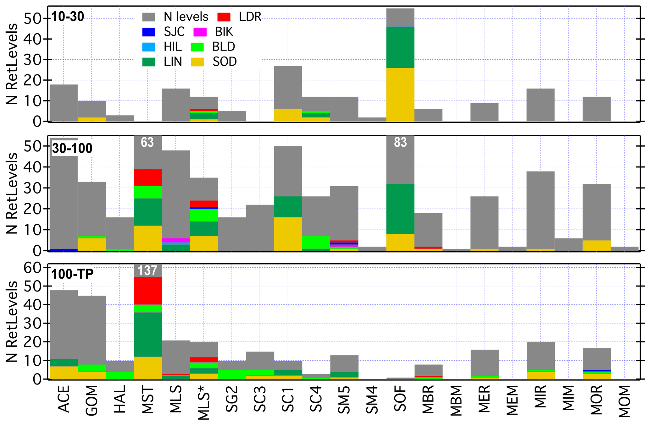
Figure 15Numbers of total reporting levels (grey) and those with large (>1 % yr−1) significant drifts at the paired FP sites (colours) for each SAT. The counts are divided into three distinct pressure intervals: 10–30 hPa, 30–100 hPa, and 100 hPa to the local tropopause (TP) pressure. Coloured bars are stacked in front of grey bars to show the fractions of reporting levels with large significant drifts across all the FP sites relative to all reporting levels. Values for the three grey bars exceeding the y-axis limits are given in white text at the top of the bar.
The pressure dependence of the drifts of each SAT–FP was investigated by separating them into three pressure intervals: 10–30 hPa, 30–100 hPa, and from 100 hPa down to the local tropopause pressure (100–TP). For the 21 SATs and 7 FP sites there were a total of 215, 604, and 394 SAT–FP time series in the 10–30, 30–100, and 100–TP pressure ranges (Fig. 15). In these pressure intervals, 76 (35 %), 209 (35 %), and 134 (34 %) of the drifts were statistically significant and 65 (30 %), 157 (26 %), and 127 (32 %) were large and significant. The uniformity of these overall percentages across the three pressure intervals suggests a general lack of pressure dependence of the significant drifts, but these bulk statistics do not provide conclusive evidence for individual SATs.
MLS∗ drifts in the 100–TP pressure interval were large and significant for 60 % of the reporting levels across its five paired FP sites (Fig. 15). In this lowest layer of the stratosphere, 50 % of the SG2 and SC1 drifts and 40 % of the HAL and MST drifts were also large and significant. Interestingly, all large significant SC1 drifts in the 100–TP interval were over SOD and LIN, while none were over BLD. For MST the highest percentages of large significant drifts (100–TP) were over LIN (50 %) and LDR (68 %). It is difficult to assess whether the large significant drifts of a specific SAT were latitude dependent in any of the pressure intervals because most SATs paired with only three or fewer FP sites.
For reporting pressures 30–100 hPa, 39 % to 69 % of the drifts of SOF, SC1, MST, and MLS∗ (in increasing order) were large and significant. All large and significant SC1 drifts were over SOD and LIN, with none over BLD, the same as for SC1 drifts in the 100–TP interval. The greatest fractions of large significant drifts for MST were again at LIN (81 %) and LDR (73 %), although there was also a high percentage at SOD (67 %). Large significant drift percentages for MLS were highest at LIN (43 %), while for MLS∗ they were 100 % at SOD and LIN, 86 % at BLD, and 43 % at LDR. The fractions of large significant SOF drifts were considerable at LIN (61 %), one of the only two FP sites with enough SOF-coincident soundings to permit statistically robust analyses of drift.
In the 10–30 hPa interval, only two SATs had large significant drifts at ≥ 50 % of their reporting levels: MLS∗ (50 %) and SOF (84 %). For MLS∗, 100 % and 50 % of drifts in this pressure range were large and significant over LIN and LDR, respectively. Large significant drift percentages for SOF were again high at SOD (84 %) and LIN (83 %). Interestingly, 55 % of the drifts in SC1 retrievals at SOD were large and significant, while none were at LIN or BLD.
Some SATs were associated with high percentages of large significant drifts at only one FP site. For GOM drifts at SOD, BLD, and LDR, 8 of the 9 large significant drifts at 43 total reporting levels in the 10–30 hPa and 30–100 hPa intervals were at SOD. In the two highest pressure intervals, 8 of 10 large significant drifts in MOR were at SOD, with 1 each at BLD and SJC and none at BIK or LDR. In the 100–TP interval, 7 of 11 large significant drifts for ACE were at SOD (48 reporting levels over 5 sites), and 4 of 5 large significant drifts for MIR were at SOD (20 levels over 4 sites). In total, 134 (38 %) and 122 (35 %) of 349 significant drifts were identified over SOD and LIN. However, when interpreting these high percentages, it should be considered that 359 (29 %) and 260 (21 %) of all the SAT–FP time series analysed for drift were over SOD and LIN, respectively.
4.4 Mean drifts for the unique SAT–FP pairs
Statistics for the drifts at all reporting levels in the same three pressure intervals are presented for each SAT–FP pair in Fig. 16. Each horizontal bar denotes the weighted average of drifts for a specific SAT–FP pair over all reporting levels in the given pressure interval, while the vertical bars depict the 95 % confidence intervals of the weighted means. Weights were calculated using Eq. (10), which scales the standard errors of drifts by the SAT-dependent compensation factors (i.e. grid width vs. vertical resolution) that were employed in the bias analyses. Uncertainties of the weighted averages were determined from the weights and the standard errors of the computed drifts using Eq. (11). The mean drift for a given SAT–FP pair is statistically significant if its 95 % confidence interval (vertical bar) does not include zero (horizontal black line at zero drift).
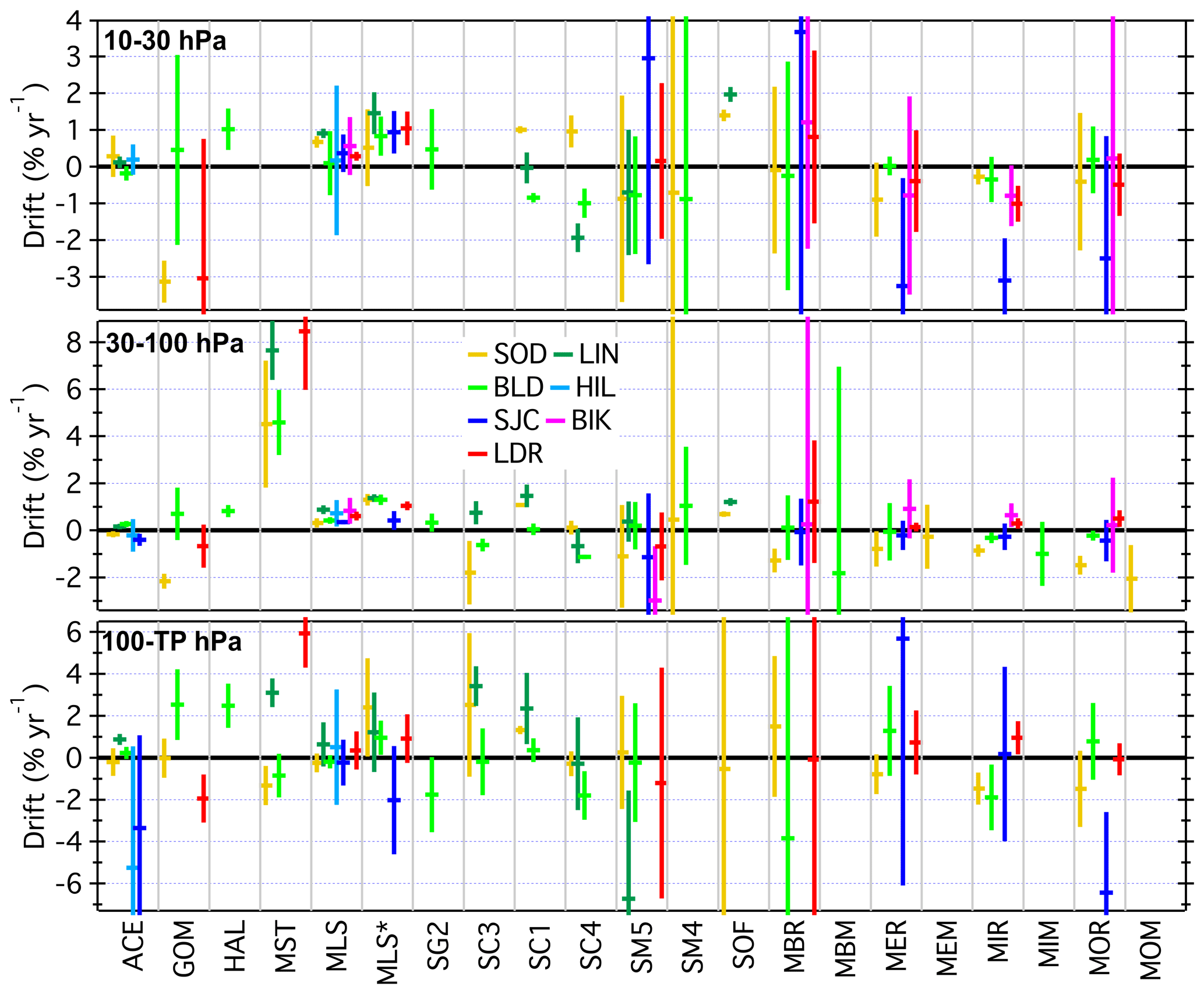
Figure 16Mean drifts (horizontal bars) and their uncertainties (vertical bars) for each SAT–FP pair across all reporting levels within each of the three pressure intervals. The x-axis bins separate results for the 21 different SATs, with colour-coded bars presenting statistics for the individual FP sites.
For some SATs there are large (>1 % in magnitude) and statistically significant mean drifts in multiple pressure intervals (Fig. 16). GOM has large negative mean drifts at SOD in both the 10–30 hPa and 30–100 hPa intervals. HAL has positive and significant mean drifts over BLD in all three pressure ranges but only those for 10–30 hPa and 100–TP are >1 % yr−1. For MST, there are large significant mean drifts in the 30–100 hPa and 100–TP intervals over LDR, LIN, and SOD. These mean drifts at LDR and LIN are positive, while those at SOD are opposite in sign. Large positive mean drifts in SC1 are indicated for all three pressure intervals at SOD and for the 30–100 hPa and 100–TP intervals at LIN. For SC4 there are large negative mean drifts in all three pressure intervals over BLD. Of the eight MIPAS retrievals evaluated here, none have large significant mean drifts in more than one of the three pressure intervals.
Another way to utilize Fig. 16 is to look for uniformity in the mean drifts of a SAT across all its paired FP sites, in one or more pressure intervals. Consistency in the drifts of a given SAT over multiple FP sites, especially those at widely separated latitudes in different hemispheres, provides evidence that the drifts are not latitude dependent. For example, the mean drifts of MLS∗ over its five paired FP sites, ranging in latitude from 45∘ S to 67∘ N, are relatively uniform in both the 30–100 and 10–30 hPa intervals (Fig. 16). Mean drifts for ACE, SC4, SM5, MBR, MER, and MIR in the 10–30 hPa range are also consistent across their paired FP sites when the uncertainties are considered. Other examples of SATs with consistent mean drifts over wide latitude ranges can be found in Fig. 16.
4.5 Mean drifts at each FP site across all SATs
When viewed across each panel of Fig. 16, uniformity in the large significant mean drifts of multiple SATs at a specific FP site (marker colour) may be indicative of a drift in the FP time series at that site rather than in the SAT time series. However, this is conclusive only if the mean drifts for a given FP site are consistent across several different SATs, not just for multiple retrievals of the same satellite instrument (e.g. MIPAS). For example, in the 10–30 hPa interval, there are relatively uniform large negative mean drifts at SJC when paired with three different MIPAS retrievals (MER, MIR, and MOR), but the mean drifts at SJC for another MIPAS retrieval (MBR) and two non-MIPAS instruments (MLS and SM5) are neither negative nor significant. Similarly, in the 30–100 hPa interval, mean drifts for SOD paired with 7 SATs are negative and statistically significant, but 5 of those 7 drifts involve MIPAS retrievals, and the mean drifts for 10 other SATs at SOD are either positive or not significantly different from zero.
This interpretation of the mean drifts shown in Fig. 16 is supported by the visible inconsistencies between the drift profiles of the various SATs paired with each FP site (Figs. 14 and B8–B9). For example, the drift profiles of GOM, MST, MLS, and SM5 at LDR (Fig. 14c) are all notably different. Similar inconsistencies between different SATs are present at other FP sites for both the non-MIPAS and MIPAS SATs. Preliminary calculations of mean drift profiles across all SATs, non-MIPAS and MIPAS SATs included, at a specific FP site, revealed that their large uncertainties rarely produce mean drifts with statistical significance. This is not surprising given the uniqueness of each SAT instrument and its retrieval methods for water vapour measurements, so no further analyses of the multiple SAT mean drifts at each FP site were performed. Such an analysis could be performed on a subset of the most stable SATs, but that would be somewhat subjective and beyond the scope of this paper.
Table 5Drift statistics in three pressure intervals for each non-MIPAS SAT across all paired FP sites. Statistically significant drifts are presented in boldface text.
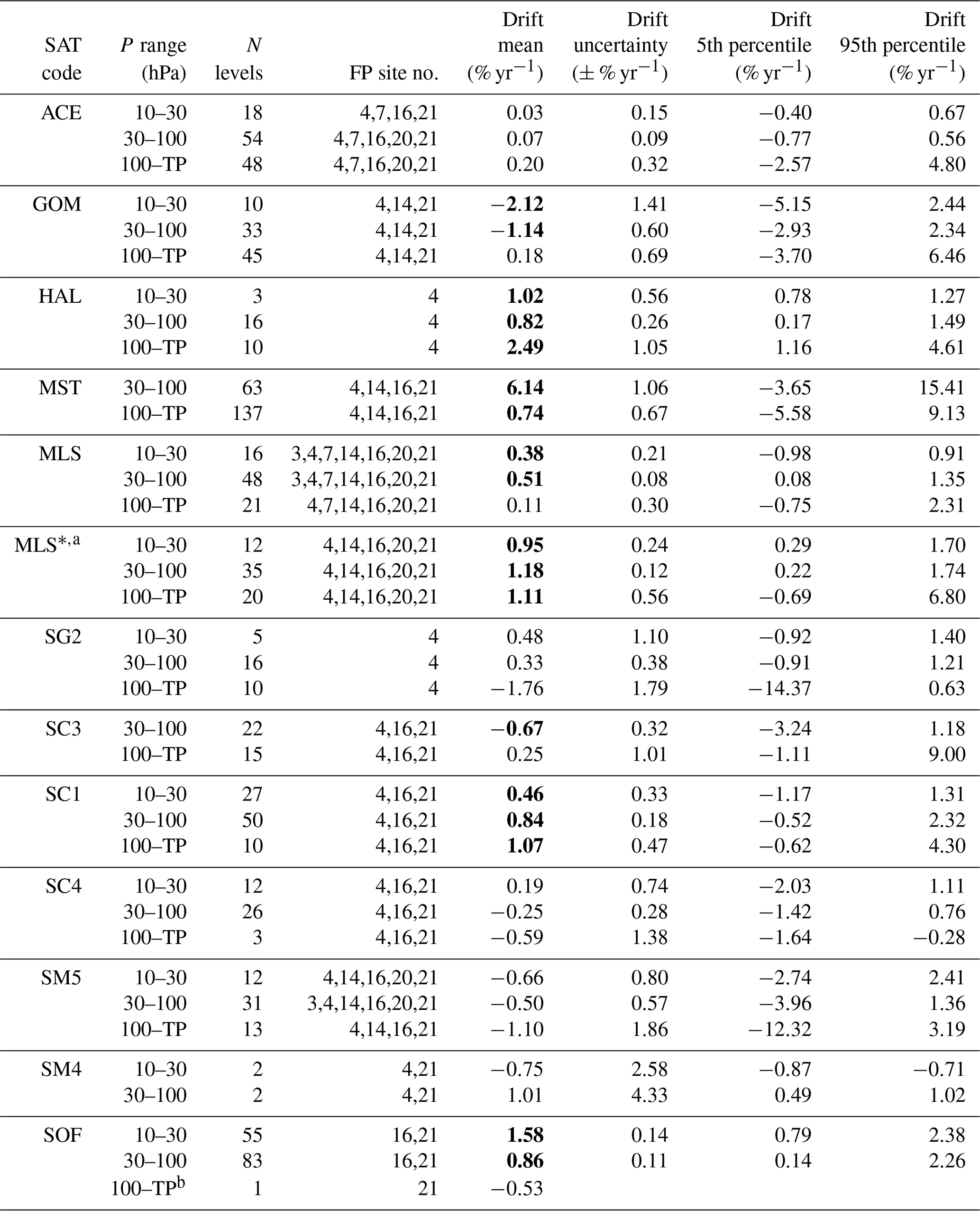
a MLS∗ is a special case for which the MLS data set is evaluated for drifts after a significant
changepoint in each time series that typically occurred in ∼ 2010 (see Sect. 4.2.1).
b No uncertainty or percentiles for the mean drift are presented because only one
time series of SOF–FP differences in the 100–TP pressure interval (at 103 hPa over SOD)
was available for drift analysis.
Table 6 Drift statistics in three pressure intervals for each MIPAS SAT across all paired FP sites. Statistically significant drifts are presented in boldface text.
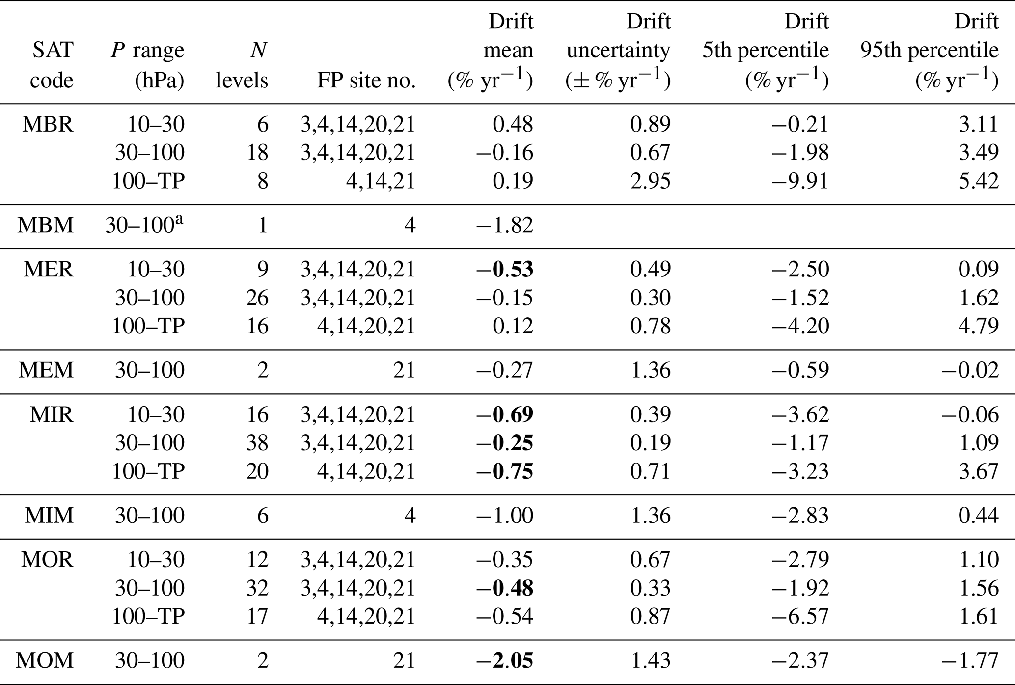
a No uncertainty or percentiles for the mean drift are presented because only one time series of MBM–FP differences in the 30–100 hPa pressure interval (at 43 hPa over BLD) was available for drift analysis.
4.6 Mean drifts for each SAT across all FP sites
Mean drifts for each SAT across all FP sites paired with it were calculated in the three pressure intervals defined above, employing the same method used to calculate the mean drifts of each unique SAT–FP pair (Fig. 16). Specifically, weighted means of drifts were computed using all the drifts in the appropriate ranges of reporting pressures, not by averaging the mean drifts at different FP sites. Averaging weights were based on the standard errors of drifts and the same SAT-dependent compensation factors employed in the site-specific mean drift computations. Uncertainties of the mean drifts of SATs across their paired FP sites were calculated from the averaging weights and standard errors of drifts using Eq. (11). Mean drifts for each SAT in the three pressure intervals are presented in Fig. 17 and listed in Tables 5 and 6.
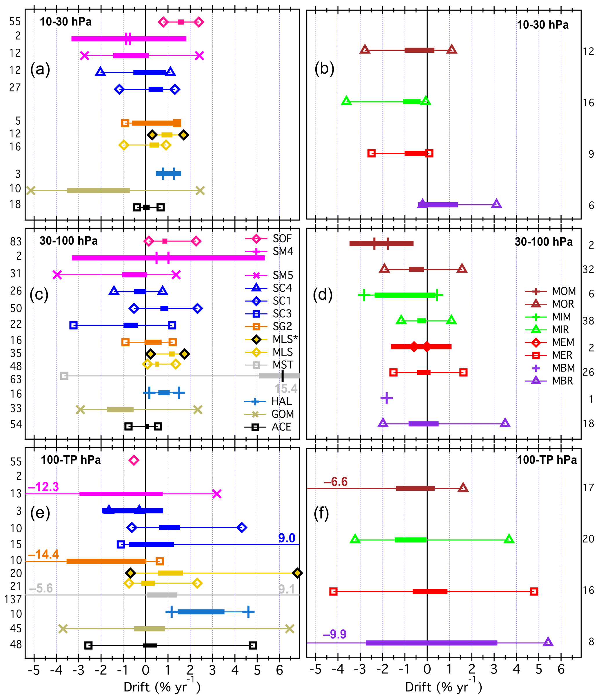
Figure 17Drift statistics for each SAT across all paired FP sites, separated into the three pressure intervals (analogous to Fig. 8 for biases). Left and right panels are for the SATs of non-MIPAS and MIPAS instruments, respectively. Mean drifts are the values at the left-to-right centres of the 95 % confidence intervals (thick horizontal bars). Markers connected by thin horizontal lines show the 5th and 95th percentiles of the drifts for each SAT. Values of 5th and 95th percentiles that exceed the x-axis limits are enumerated as coloured text. In some cases, markers for the 5th and 95th percentiles are well within the 95 % confidence intervals because of large Student t values for data sets with small populations. In the left 30–100 hPa panel, a small black vertical bar denotes the mean drift for MST. Only a mean drift value is presented for SOF (100–TP) and MBM (30–100) because only one retrieval pressure for each provided time series of differences met the criteria for drift analysis. Values presented to the left of the left panels and to the right of right panels indicate the number of retrieval levels with difference time series that were used to determine the statistics shown.
Figure 17 is analogous to Fig. 8 except it presents statistics for drifts instead of biases. Here, each thick horizontal bar represents the 95 % confidence interval of the mean drift. Since these confidence intervals are symmetric about the mean, the value at the centre of each thick horizontal bar is the mean drift. Thin horizontal lines show the inter-90 % range of drifts, with markers denoting the 5th and 95th percentiles. In the text below, the terms “variability” and “range” are used when discussing the 95 % confidence intervals (e.g. variability of ±x % yr−1) and inter-90 % ranges (e.g. range of y to z % yr−1).
4.7 Synopsis of the drift assessments
A brief statistical synopsis of the drifts in the three pressure intervals for each SAT is now presented, including relevant information about the fractions of reporting levels with large and statistically significant drifts and, where possible, statements about the uniformity, signs, and magnitudes of drifts in specific pressure intervals. In most cases the information can be visually confirmed in one of more of Figs. 15, 16, and 17. Drifts for the 12 non-MIPAS retrievals are discussed first and then drifts for the 8 different MIPAS retrievals.
ACE
Drifts for ACE were large and statistically significant at 12 of the 120 (10 %) reporting levels over its 5 paired FP sites, of which 11 were at pressures >100 hPa over SOD and LIN. However, in this pressure range, only the mean drift at LIN was significant (Fig. 16). In the 30–100 hPa interval, only one drift at 54 reporting levels was large and significant over SOD, LIN, BLD, HIL, and SJC. Across all paired FP sites, ACE drifts spanned a wide range in the 100–TP interval, but the variability was much smaller and the mean drift was not statistically different from zero (Fig. 17). In the two pressure intervals ≤ 100 hPa, both the variability and ranges of drifts across all sites were small and the mean drifts were not statistically significant.
GOM (GOMOS)
Of the 16 large and statistically significant drifts at 88 GOM reporting levels over its 3 FP sites (SOD, BLD, LDR), 12 were over SOD and 4 were over BLD. There were significant negative mean drifts in the 10–30 and 30–100 hPa intervals over SOD (Fig. 16) because drifts at all 13 reporting pressures were negative and 8 were large and significant. Of the 11 reporting levels over BLD in the 100–TP interval, 9 were uniformly positive, of which 3 were large and significant, yielding a significant positive mean drift. Several large negative drifts in the 100–TP range over LDR resulted in a significant negative mean drift. Mean drifts across all three sites were negative and significant in the 30–100 and 10–30 hPa intervals but not in the 100–TP interval (Fig. 17).
HAL (HALOE)
Measurements by HAL ceased in mid-November 2005, so its record has a >5-year overlap with only the FP record at BLD. The HAL instrument began measurements in October 1991, but only the last 5.9 years of its record (since January 2000) are analysed here since the first WAVAS report covered HAL data through 1999 (Kley et al., 2000). Though large and significant drifts were determined for only 5 of 29 reporting levels, all 29 drifts were positive and relatively uniform. This uniformity resulted in positive and significant mean drifts of 0.8±0.3 % yr−1 to 2.5±1.0 % yr−1 over BLD in all three pressure intervals.
MST (MAESTRO)
The MST data analysed here cover 200 reporting pressures over four FP sites but only as high as 33 hPa. Large significant drifts were determined for 94 (47 %) reporting levels, with 39 and 55 in the 30–100 and 100–TP intervals, respectively. MST time series were not available at pressures ≤ 30 hPa for drift analysis. Drifts were large and significant at 23 of 33 (70 %) reporting levels over LDR (Fig. 10d) and 37 of 64 (58 %) reporting levels over LIN (Fig. B3h). Between these two sites, 94 % of all MST drifts were positive, producing large significant mean drifts at LIN and LDR in the 100–TP and 30–100 hPa ranges (Fig. 16). Drifts over SOD and BLD were large and significant at 40 % and 23 % of all reporting levels (Fig. B3d, l), with 17 of 18 large significant drifts being positive in the 30–100 hPa range over both sites and 12 of 16 large significant drifts being negative in the 100–TP interval. Consequently, over SOD and BLD there were significant positive mean drifts in the 30–100 hPa interval and negative mean drifts in the 100–TP interval, of which the SOD mean drift was significant. Mean MST drifts across all four FP sites were positive and significant in both the 30–100 and 100–TP intervals (Fig. 17).
MLS and MLS∗
Drifts were calculated separately for the full MLS records (2004–2016) at all seven FP sites and for shorter records from their changepoint dates (∼ 2010) through 2016 (represented by MLS∗) at all sites except HIL and BIK. Across their paired FP sites, drifts for full MLS records and MLS∗ were large and significant at 9 (11 %) of 85 reporting levels and 42 (63 %) of 67 reporting levels, respectively. In the 30–100 hPa range, the mean drifts for MLS and MLS∗ across their paired FP sites were positive and significant, as were their mean drifts in the 10–30 hPa interval (Fig. 17). In the 100–TP range, mean drifts for MLS and MLS∗ across their paired FP sites were weakly positive and not significant, and strongly positive and significant, respectively. Figures 16 and 17 show not only the uniformity of the MLS and MLS∗ mean drifts across their associated FP sites, but also how the MLS drifts in the 10–30 and 30–100 hPa intervals increase by 120 %–140 % when they are determined for the shorter post-changepoint records (MLS∗) instead of the full records (MLS).
SG2 (SAGE II)
SAGE II measurements began in September 1984 and ended in mid-2005, but only the SG2–BLD time series spanning 2000 through mid-2005 are analysed here for drift. Large significant negative drifts were found for 5 of the 10 reporting levels in the 100–TP interval (Fig. B3m), but the mean drift was not significant. None of the drifts at pressures ≤ 100 hPa were significant, and neither were the mean drifts for the 30–100 hPa and 10–30 hPa intervals (Fig. 17).
SC3 (SCIAMACHY limb)
Drifts were large and significant at only 5 of 37 reporting levels over SOD, LIN, and BLD, and all 5 were in the 100–TP interval (Fig. B3b, f, j). However, relatively uniform positive drifts at 11 of 12 reporting levels in the 100–TP and 30–100 hPa intervals over LIN produced significant positive mean drifts (Fig. 16). SC3 time series were not available at pressures ≤ 30 hPa for drift analysis. Interestingly, drifts over SOD and BLD in the 30–100 hPa range were negative at 14 of 15 reporting levels, resulting in significant negative mean drifts. Across the three FP sites, there was a significant negative mean drift in the 30–100 hPa interval.
SC1 (SCIAMACHY solar OEM)
Drifts over SOD at 24 of 31 (77 %) reporting levels were uniform, positive, large, and significant (Fig. 10a), as were the mean drifts over SOD for all three pressure intervals. Drifts at all 13 SC1 reporting levels >50 hPa over LIN (Fig. B3e) were also uniform, positive, large, and significant, as were the mean drifts in the 100–TP and 10–30 hPa intervals. Over BLD, none of the drifts at all 28 reporting levels were large and significant, yet the uniformly negative drifts at the eight levels ≤ 30 hPa produced a significant negative mean drift in the 10–30 hPa range. SC1 mean drifts across the three sites were positive and significant for all three pressure intervals (Fig. 17).
SC4 (SCIAMACHY solar OP)
Drifts over BLD were uniformly negative at all 13 reporting pressures and large and significant at 10 levels (Fig. B3k), producing significant negative mean drifts for all 3 pressure intervals (Fig. 16). Mean drifts in the 10–30 hPa range over LIN and SOD were also significant but of opposite sign. Mean drifts in the 100–TP range were based on only one reporting pressure at each site, and only the negative drift at 115 hPa over BLD was significant. The mean drift across all three sites was statistically different from zero only for the 30–100 hPa interval.
SM5 (SMR 544 GHz)
Only 9 of the drifts at 56 reporting levels across 6 paired FP sites were large and significant, and these were dispersed across the 6 sites. At LIN, three large significant negative drifts in the 100–TP interval produced a large significant negative mean drift. Mean drifts at each FP site were relatively uniform in all three pressure intervals, but none of the mean drifts across the FP sites were significant.
SM4 (SMR 489 GHz)
Drifts were determined at only four SM4 reporting pressures over two FP sites: SOD (23 and 35 hPa) and BLD (21 and 33 hPa). No drifts were statistically significant. With only one reporting pressure per site in each of the 10–30 and 30–100 hPa pressure ranges, the two mean drifts for each site have large uncertainties and are therefore not significant. Similarly, mean drifts across the two FP sites were highly uncertain and not statistically significant (Fig. 17).
SOF (SOFIE)
Vertical profiles of drifts at SOD and LIN were similar (Fig. B3n,o), with large significant positive drifts at 76 of the 100 combined reporting pressures between 14 and 60 hPa. Drifts in the 30–100 hPa and 10–30 hPa intervals over each site were fairly uniform and positive, producing significant positive mean drifts for SOD and LIN (Fig. 16). Over the two sites, there was only one reporting pressure in the 100–TP range, and this singular drift at 103 hPa over SOD was highly uncertain and not significant. Therefore, mean drifts across the two FP sites were not significant in the 100–TP interval but positive and significant in both the 30–100 and 10–30 hPa intervals.
MBR and MBM (MIPAS Bologna V5R NOM and MA)
Drifts of MBR, large and significant at only 4 of 32 reporting levels over five FP sites, were dispersed across three sites (Fig. B4). Only the mean drift at SOD in the 30–100 hPa interval was significant, the result of uniform negative drifts at all five reporting levels (Fig. B4a). One large, significant negative drift in the 100–TP interval over each of BLD and LDR substantially increased the variability and range of drifts over all sites (Fig. 17). For MBM, the drift was not significant at 43 hPa over BLD, the only MBM time series analysed for drift, so the resulting mean drift was highly uncertain and not significant.
MER and MEM (MIPAS ESA V7R NOM and MA)
There were 3 large and significant drifts at 51 MER reporting levels scattered over five sites (Fig. B5). In general, drifts were not uniformly positive or negative in any of the pressure intervals over any site except for the two reporting levels ≤30 hPa above SJC and for four of five reporting levels in the 30–100 hPa interval above SOD. Significant negative mean biases were determined for both. The variability of MER drifts across all sites was small in each pressure interval. Drift results for MEM were available for only two reporting pressures over SOD: 34 and 52 hPa. Neither drift was significant or resulted in a significant mean drift for the 30–100 hPa interval.
MIR and MIM (MIPAS IMK/IAA V5R NOM and MA)
There were six large and significant drifts at the 74 MIR reporting levels over five FP sites, and all were negative (Fig. B4). Five were over SOD, of which four were in the 100–TP interval, producing a significant negative mean drift. In the same pressure range, there were fairly uniform positive drifts at all seven reporting levels over LDR and negative drifts at four of five reporting pressures over BLD, including one large, significant negative drift, and these produced significant mean drifts at both sites (Fig. 16). In the 30–100 hPa range, mean drifts over SOD, BLD, BIK, and LDR were significant due to relatively consistent but rarely significant negative (SOD, BLD) and positive (BIK, LDR) drifts. Similarly, consistent negative drifts at the 2–4 MIR reporting levels in the 10–30 hPa range over each of SOD, SJC, and LDR resulted in significant negative mean drifts. Across the five FP sites, mean drifts for MIR were negative and significant in all three pressure intervals (Fig. 17). For MIM, only six time series of differences in the 30–100 hPa range over BLD were analysed. None of the six drifts or the mean drift for 30–100 hPa were statistically significant.
MOR and MOM (MIPAS Oxford V5R NOM and MA)
Drifts in MOR retrievals were large and significant at 10 of 61 levels over five FP sites, of which eight were negative and over SOD (Fig. B5). Five of the eight significant negative drifts over SOD were in the 30–100 hPa range, producing a significant negative mean drift (Fig. 16). Consistent positive drifts at five of six reporting levels in the same pressure interval over LDR resulted in a positive significant mean drift. At SJC, there was a large significant negative drift at the lone reporting pressure >100 hPa, so the mean drift was significant and negative (Fig. 16). In the 10–30 hPa pressure interval, none of the individual or mean drifts over the five FP sites were significant, so neither was the mean drift across all five sites. There was a significant negative mean drift at SOD and across all five FP sites in the 30–100 hPa pressure interval due to the five large and significant negative drifts over SOD. For the two MOM reporting pressures in the 30–100 hPa range over SOD, neither of the negative drifts were significant, but they were large and consistent enough to produce a significant negative mean drift.
We have compared satellite data records of stratospheric water vapour recorded since 2000 to FP profiles from 27 stations spanning a wide range of latitudes (45∘ S to 79∘ N). For the comparison, we applied the same approach to all satellite data products. In particular, we applied a priori and averaging kernels of the satellite data to the FP profiles in order to adjust them to the retrieval characteristics of each satellite data set. If averaging kernels were not available, we smoothed the FP profiles with ad hoc Gaussian-shaped smoothing kernels to account for the vertical resolution of the satellite instruments. Two consistent sets of collocation criteria were utilized based on two classes of instruments: for the dense samplers we used a time difference <24 h, a distance <1000 km, and a latitudinal difference <5∘, while for occultation instruments we used 7×24 h, 2000 km, and latitudinal difference <15∘.
We determined the profiles of the biases and drifts and their uncertainties (in terms of the standard error of the mean, SE, and of the linear regressions fits) of every instrument versus each FP station by averaging over all available collocations. By analysing the bias and drift profiles of one satellite instrument across all hygrometer stations, we obtained insight into the general behaviour of the satellite instruments, including general information indicating an absence of obvious latitudinal dependencies of their biases and drifts. Similarly, a comparison of all satellite instruments to each specific FP station provided some insight into any peculiarities of the FP record at each station. We have concentrated on the satellite data analysis and have, as a final synopsis of the comparisons, averaged the biases and drifts of each individual satellite instrument over all FP stations within three different pressure ranges, namely 10 to 30 hPa, 30 to 100 hPa, and 100 hPa to the local tropopause pressure.
Most SAT data records have biases <10 % and drifts <1 % yr−1 relative to FPs that are considered the most accurate and best-characterized instruments for the measurement of stratospheric water vapour. Satellite instruments with biases below 10 % over the complete altitude range analysed here are ACE, MLS, SG2, SG3, SC4, MBR, MER, MIH, MIR, MOH, and MOR. SATs with mean drifts <1 % yr−1 in all three pressure intervals were ACE, MLS, SC4, MBR, MER, MIR, and MOR. Of the 1213 time series of relative differences between 21 SATs and 7 FP sites that were analysed for drifts, 419 (35 %) had statistically significant drifts at the 95 % level of confidence. Of these 419 significant drifts, 349 (83 %) were also large drifts, with magnitudes >1 % yr−1. Five SATs were together associated with 76 % of the large significant drifts: MLS∗, SOF, MST, SC1, and SC4. Eleven SATs had large significant drifts at 15 % or less of their reporting levels: ACE, MLS, SC3, SM4, MBR, MBM, MER, MEM, MIR, MIM, and MOM. GOM, HAL, MST, and MOM had mean drifts with magnitudes >2 % yr−1 in one pressure interval, which makes their measurement time series unsuitable for the detection of stratospheric water vapour trends as large as 20 % per decade.
In the 10 to 30 hPa range, most satellite data have a relative bias within the ± 10 % range versus the mean of all FP data. Exceptions are GOM, ILA, HIR (however, the latter two are close to −10 %), MST (which does nominally not measure in this altitude range), SLA, SLB, and SM5 (nominally restricted to the upper troposphere and lower stratosphere). Among the well-performing instruments, ACE, MBR, MBM, MER, MIM, MOR, MOM, MLS, SG2, SC1, SC4, and SOFIE have biases within the ± 3 % range. Also in the 10–30 hPa interval there were eight SATs with statistically significant mean drifts across all of their associated FP sites, but of these only GOM, HAL, and SOF had large significant mean drifts (>1 % yr−1). Of the SATs that reported data in this pressure range, ACE, HAL, MLS, SG2, SM5, SM4, MBR, MER, MIR, and MOR had no large significant drifts at any of their reporting levels.
The 30 to 100 hPa range is where most instruments perform best. Only GOM, MST, MEH, MEM, MOM, POM, SLA, and SM5 show biases larger than 10 % (while GOM and POM are close to ± 10 %, and MST does nominally not cover this altitude range). The least biased water vapour data records in this altitude range are ACE, HIR, MLS, SG3, SC4, SOF, MBH, MBR, MER, MIH, and MIR, again with biases within the ± 3 % range. SG2 and MOR just miss the ± 3 % mark. All 21 SATs provided data for drift analysis at one or more pressure levels in the 30–100 hPa interval over at least one FP site. Most SATs had their smallest mean drifts in this pressure range relative to those above and below. Mean drifts were significant for 11 SATs in this pressure range, but only those for GOM, MST, MLS∗, and MOM were large and significant.
The situation is worse in the 100 hPa to tropopause range. Here, most instruments have larger biases and drifts. Nevertheless, the following SATs have biases within the ± 10 % range even in this altitude range: MLS, ACE, SC4, SG2, SG3, GOM, POM, MOR, MOH, MBR, MBH, MER, MIR, and MIH. The biases are significant for almost all data sets in the three altitude ranges in the sense that the range ±2σb, i.e. twice their SE (thick horizontal bars in Fig. 8), around the bias does not include zero. The large numbers of collocations that were available in most cases result in this high proportion of bias significance. The 5th and 95th percentiles, however, are very wide in most cases, which indicates a large spread in the individual bias profiles. Mean drifts in the 100–TP pressure interval were almost always associated with larger uncertainties than those for the two pressure ranges above. Consequently, only 34 % of the mean drifts in this interval were significant, but 95 % had magnitudes >1 % yr−1. Overall, only five SATs had significant mean drifts and three of these (HAL, MLS∗, SC1) were large and significant.
In summary, these assessments of mean biases and drifts against FP profiles from a widespread, worldwide array of FP sites demonstrate that the satellite data records are generally very valuable sources of information on atmospheric water vapour abundance from the tropopause to about 30 km altitude (10 hPa pressure). Even with their inherent biases and drifts, these satellite records have the advantages of near-global coverage and higher spatial and temporal data densities relative to the current sparse network of FP sites. Though independently valuable within their data density limitations, the network of FP sites provides “reference points” to which the satellite data sets can be anchored. In this sense, the optimal observation system for stratospheric water vapour is based on simultaneous measurements by both types of instruments, with any detected discrepancies between them being critical information.
Finally, continuing efforts to improve stratospheric water vapour measurements include the refinement of satellite retrieval algorithms, even for instruments that are no longer operational. Indeed, new data sets have been produced since 2017 for some of these satellite instruments. Obviously, the information provided by this type of assessment is invaluable to satellite instrument teams but will almost always lag behind the most current data sets. Therefore, we recommend routinely performing these assessments at least every 10 years.
A1 Biases per SAT data set
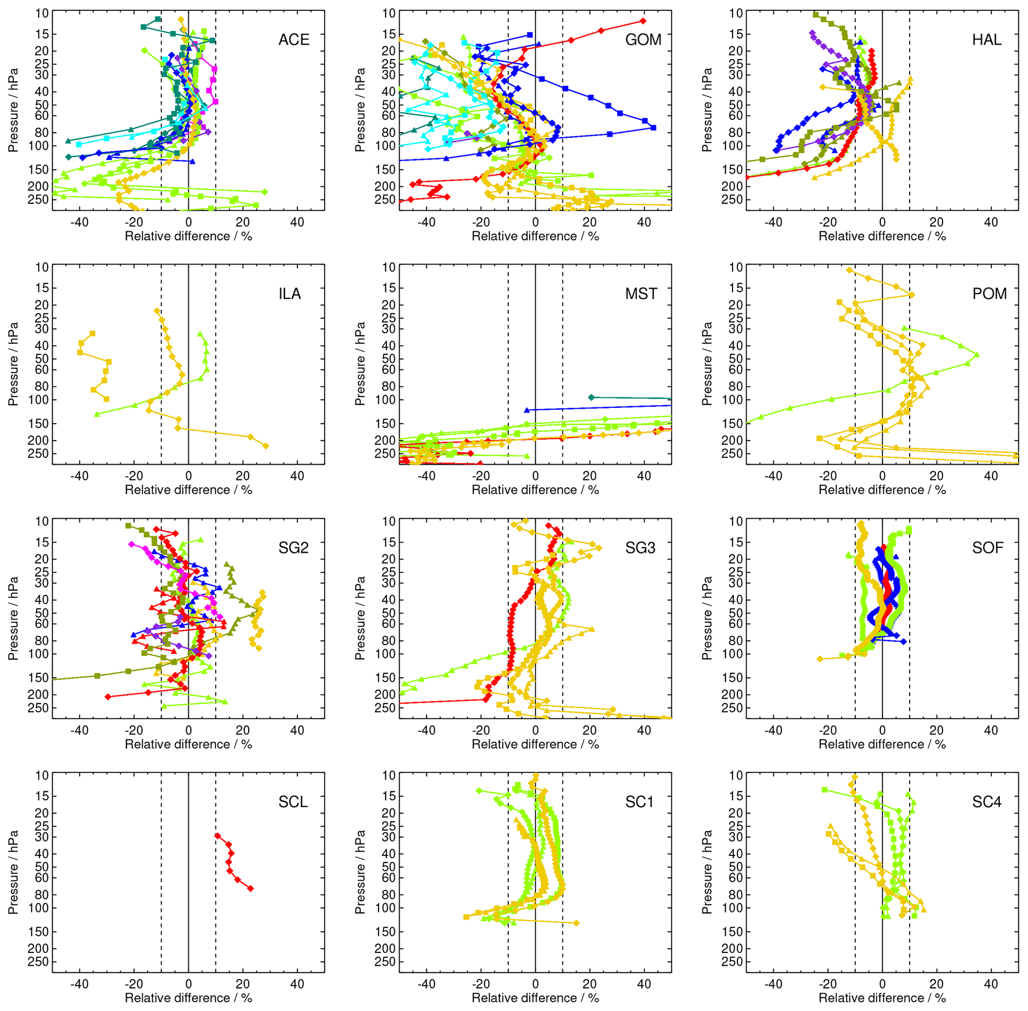
Figure A1Mean relative differences between coincident SAT (no MIPAS) and FP records. Colour coding of FP data according to Fig. 1.
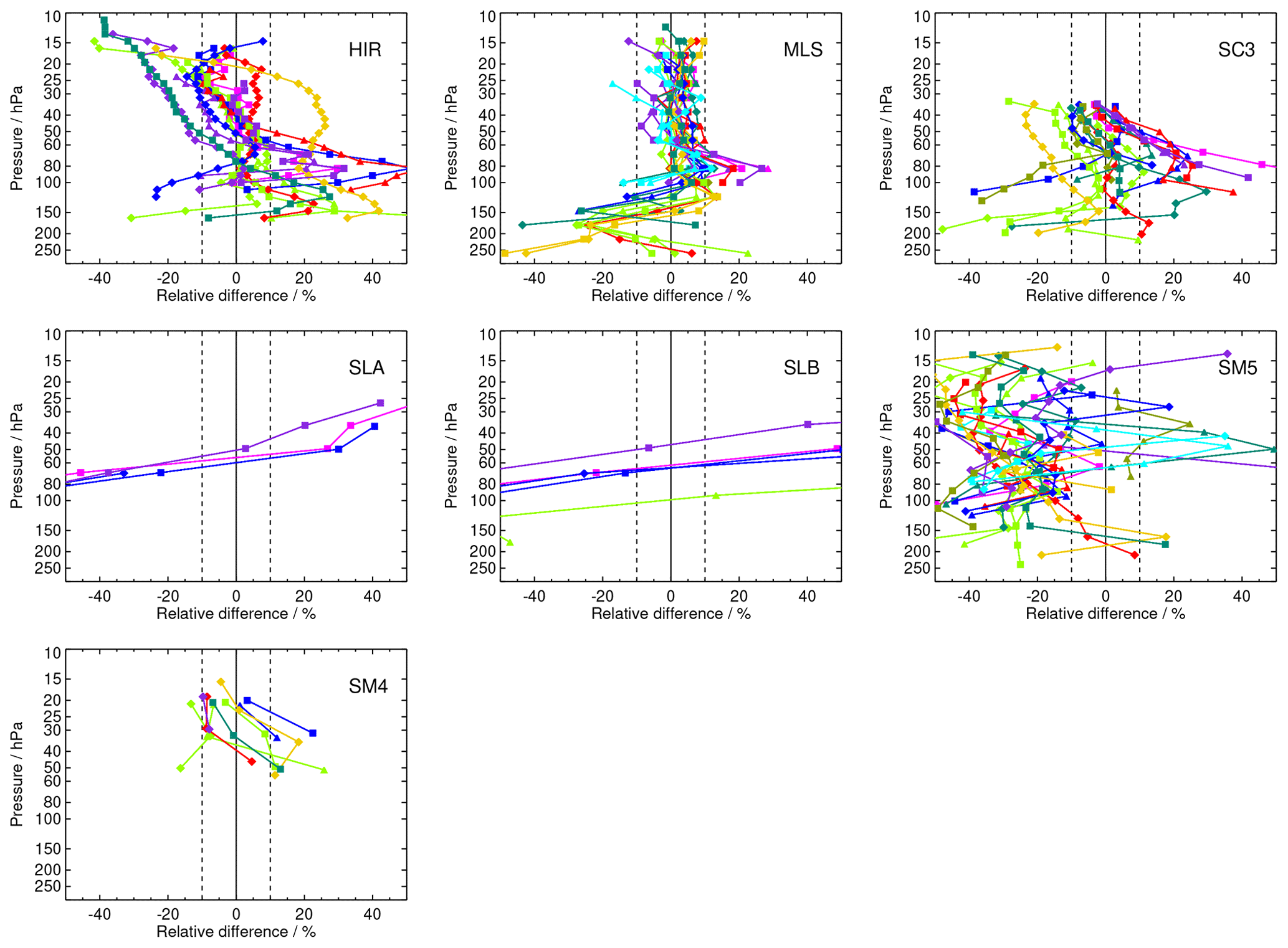
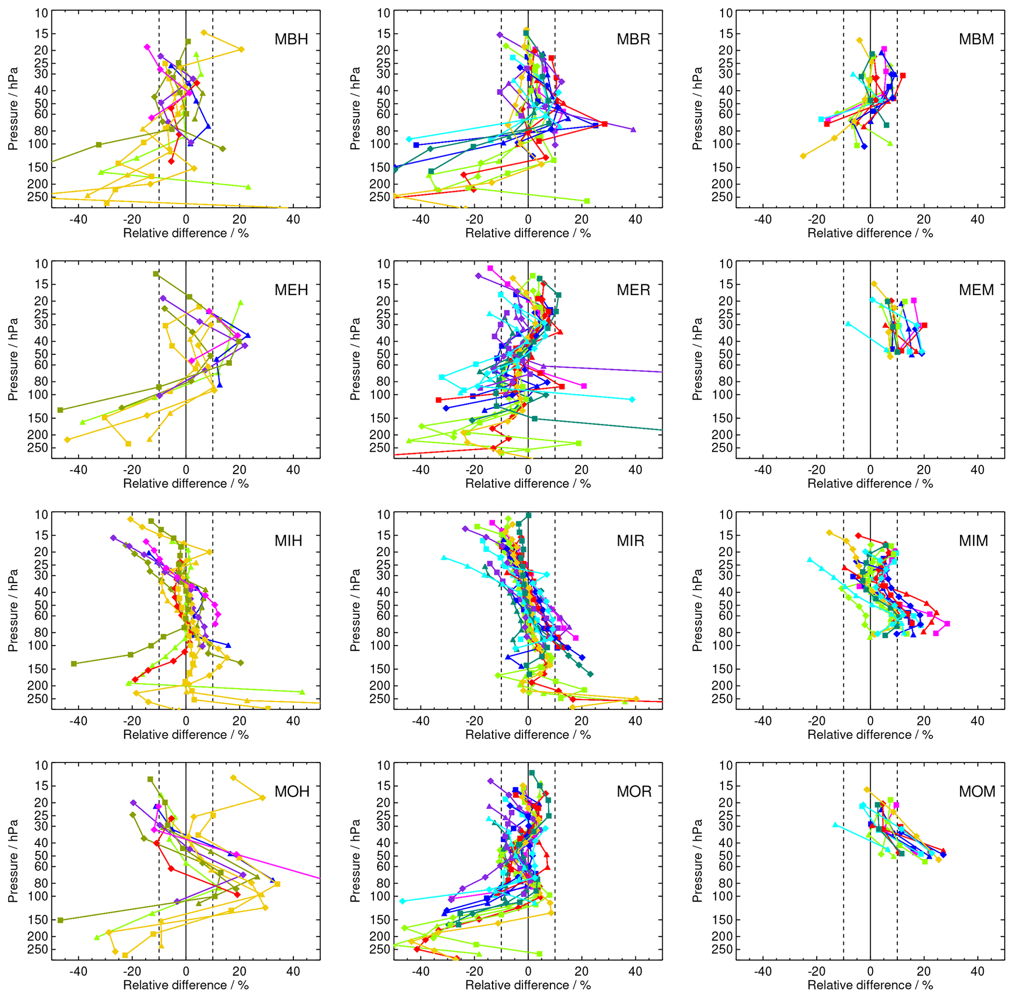
A2 Biases per FP data set, ordered by latitude
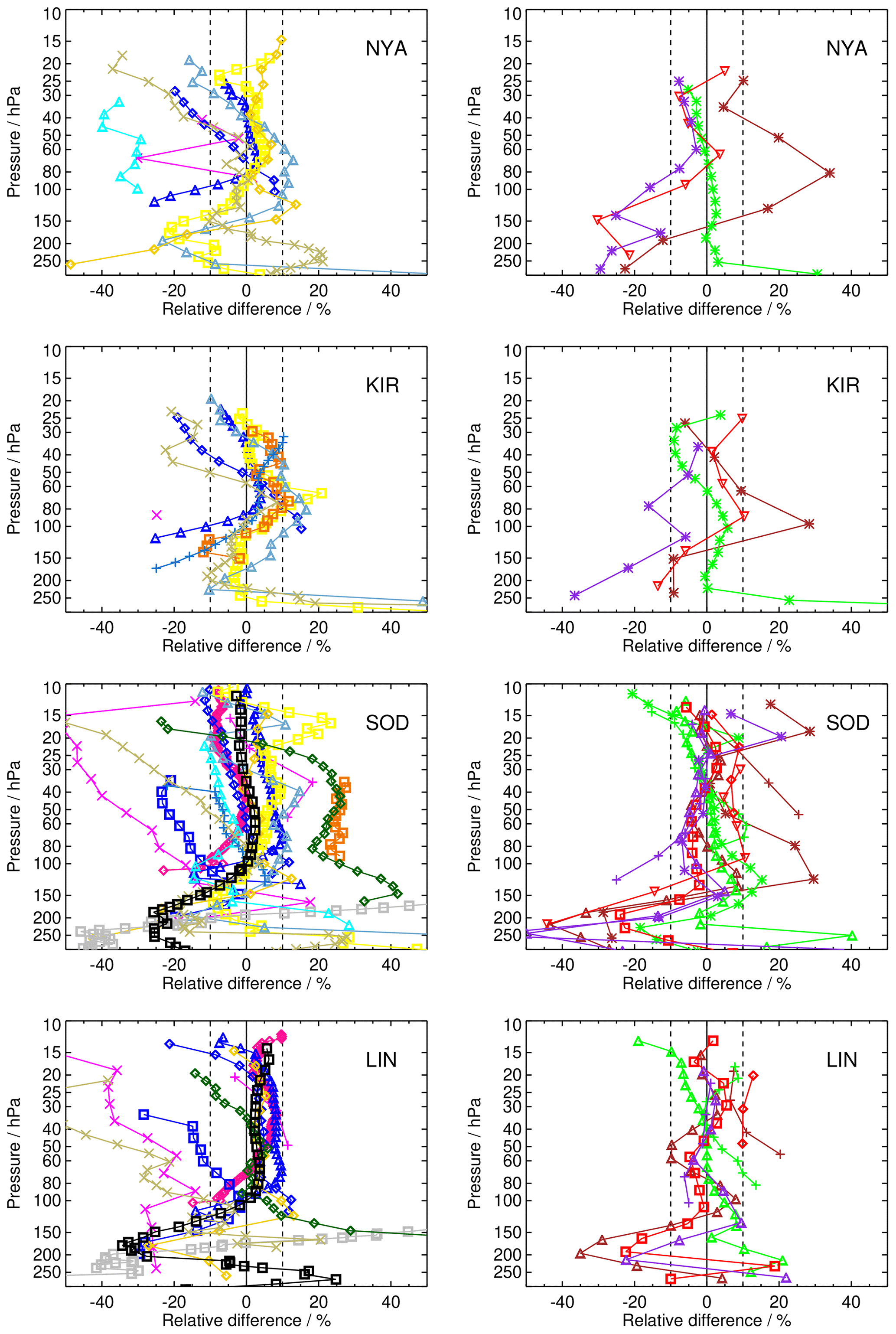
Figure A4Mean relative differences between the FP stations NYA, KIR, SOD, LIN, and coincident SAT records (left: data records except MIPAS; right: only MIPAS data records). Colour coding of the SAT data according to Fig. 2.
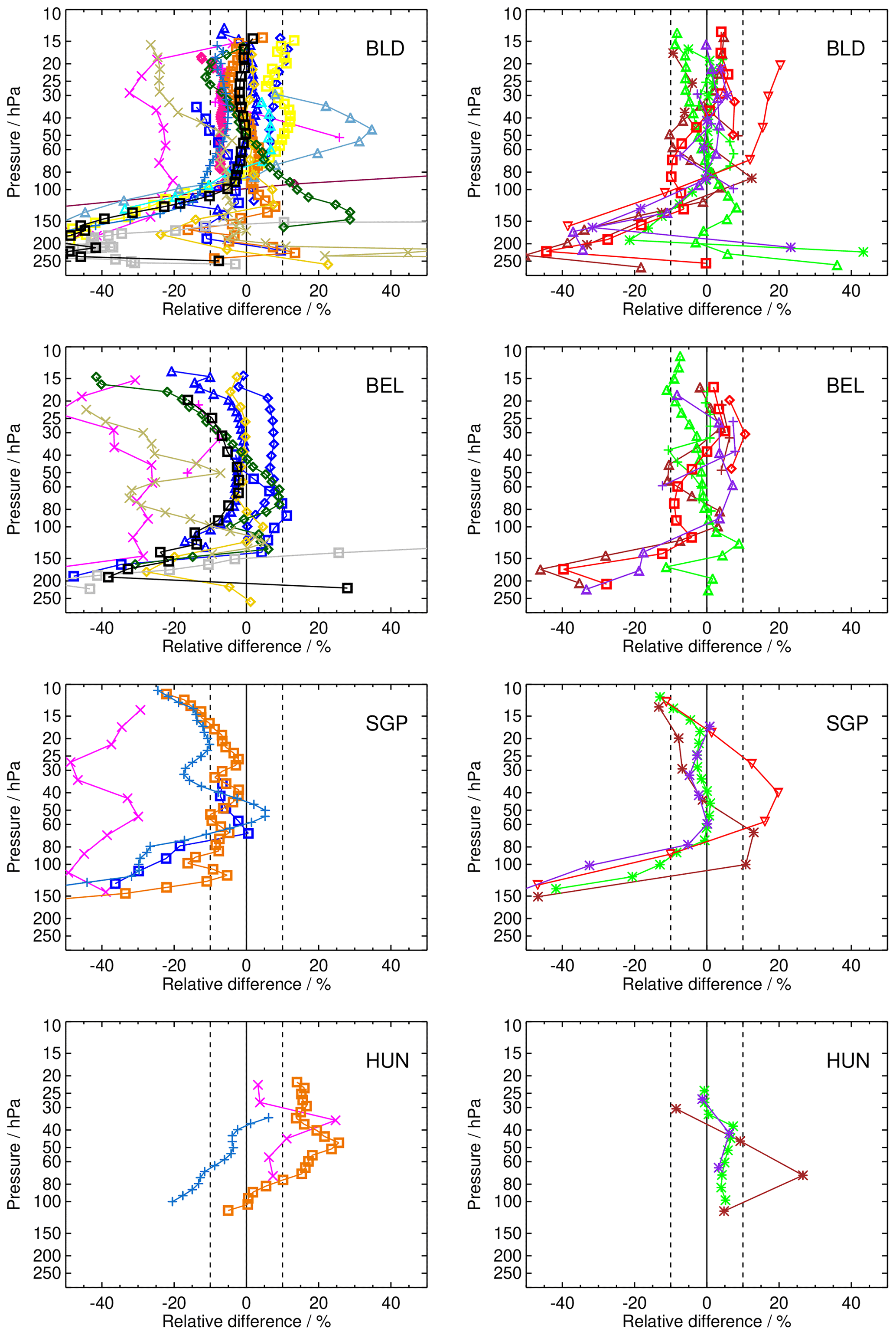
Figure A5Same as Fig. A4 but for BLD, BEL, SGP, and HUN (left: non-MIPAS, right: MIPAS only).

Figure A6Same as Fig. A4 but for FTS, TMF, LSA, and HOU (left: non-MIPAS, right: MIPAS only).
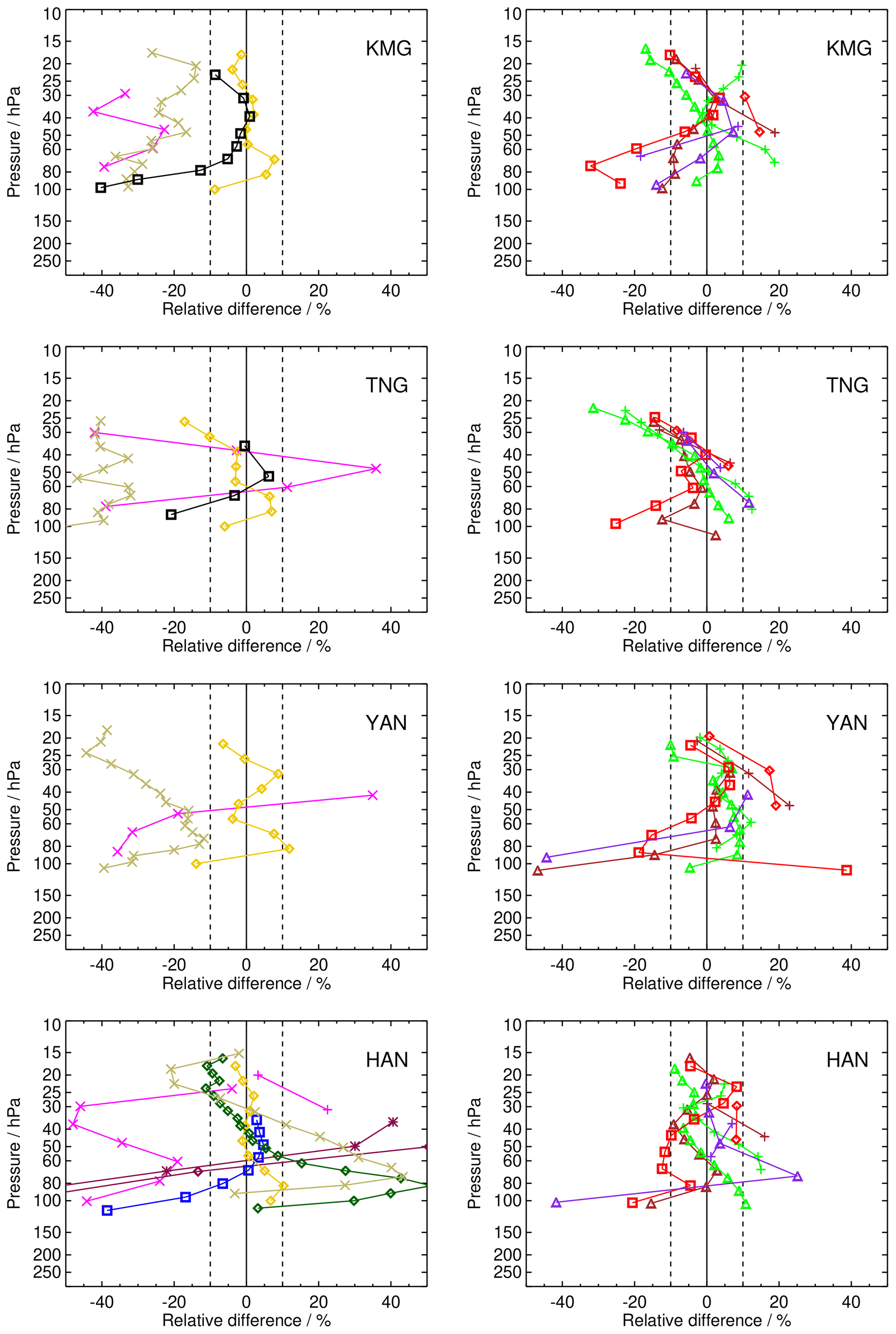
Figure A7Same as Fig. A4 but for KMG, TNG, YAN, and HAN (left: non-MIPAS, right: MIPAS only).
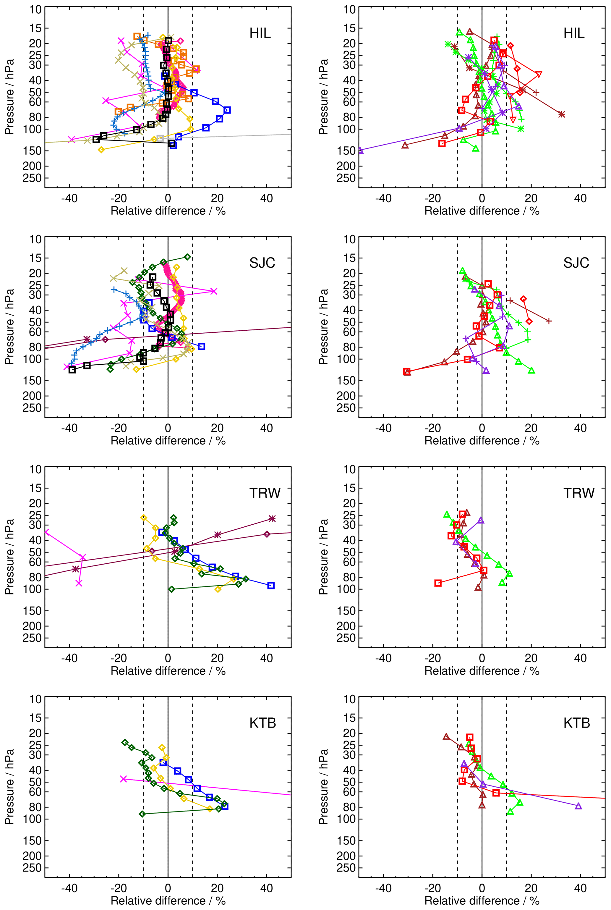
Figure A8Same as Fig. A4 but for HIL, SJC, TRW, and KTB (left: non-MIPAS, right: MIPAS only).
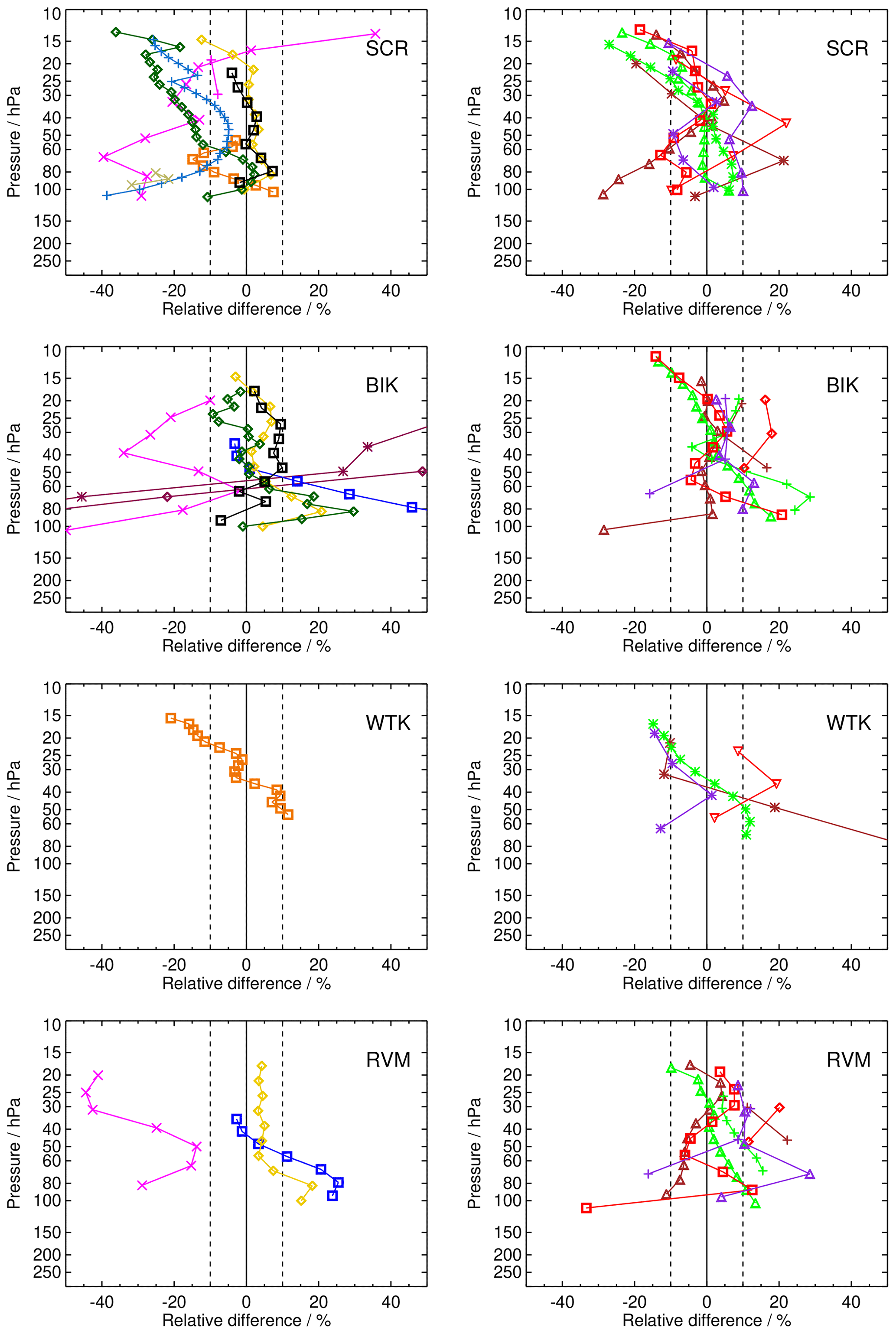
Figure A9Same as Fig. A4 but for SCR, BIK, WTK, and RVM (left: non-MIPAS, right: MIPAS only).
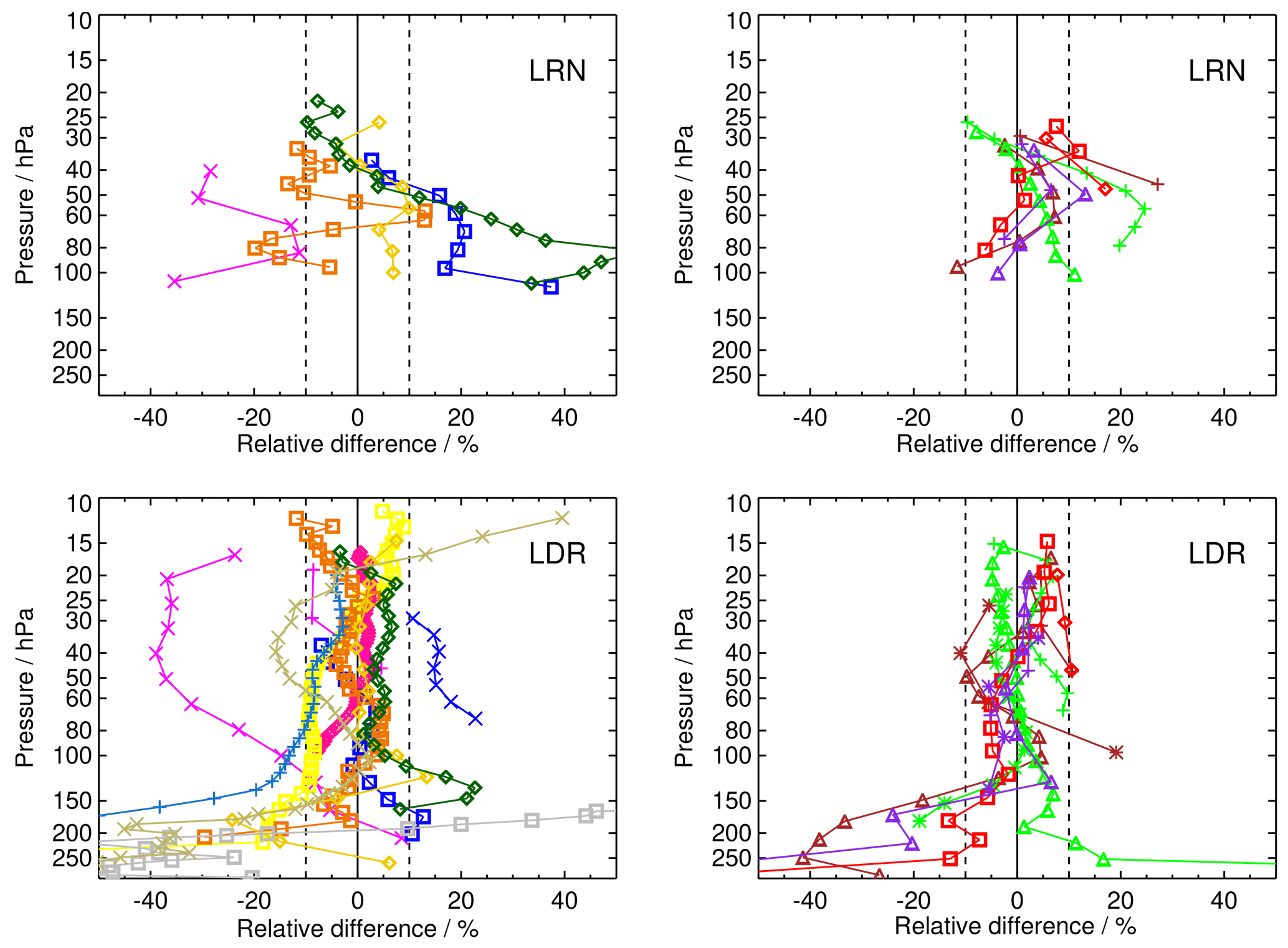
B1 Drift profiles for every SAT–FP pair
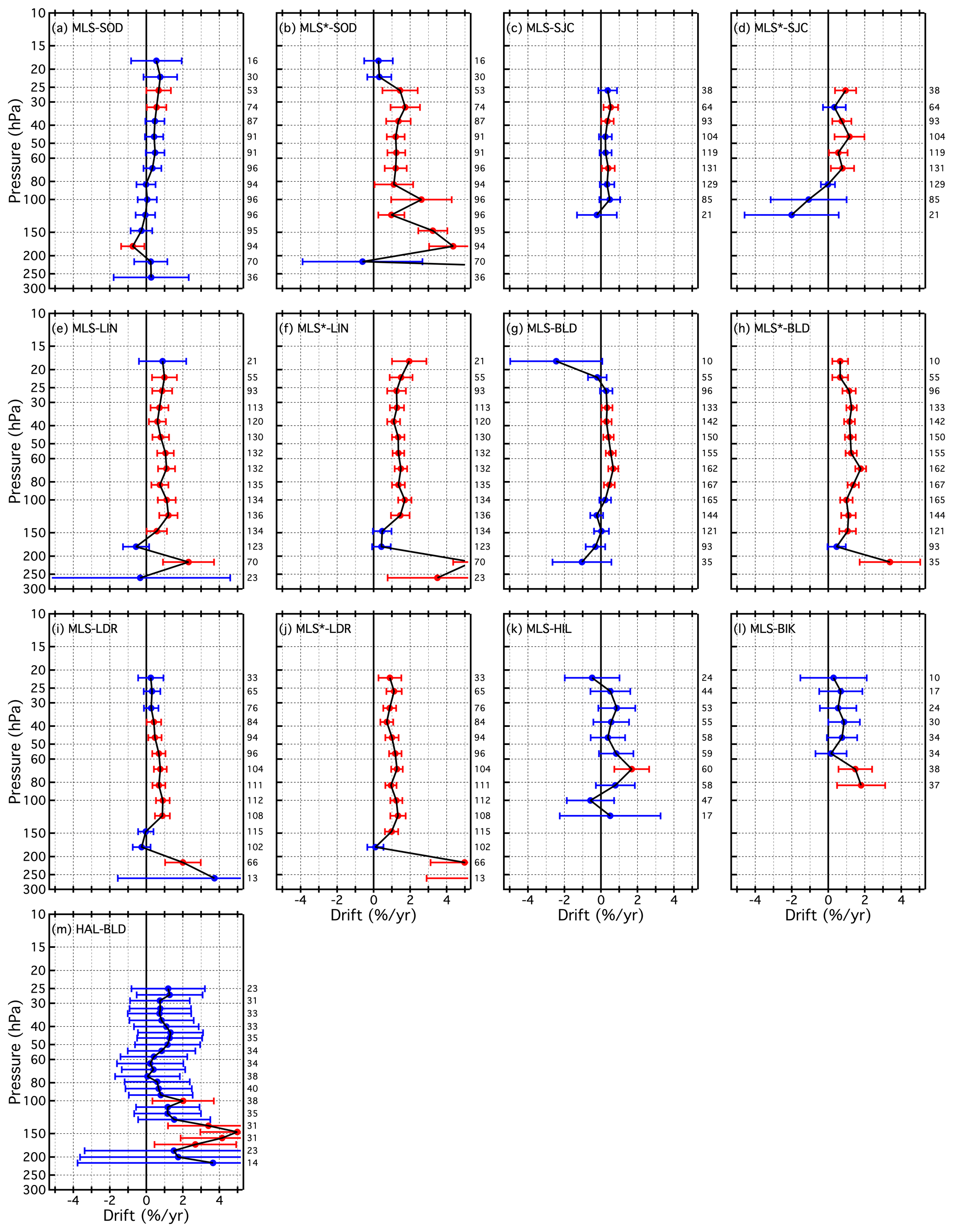
Figure B1Vertical profiles of drifts (filled circles) and their 95 % confidence intervals (horizontal error bars) for 13 different SAT–FP pairs that include MLS, MLS∗, and HAL. Blue error bars denote drifts that are not significantly different from zero, while red error bars indicate statistically significant drifts. Numbers in black text to the right of each panel present the number of SAT–FP differences in the time series analysed for drift at the corresponding pressure levels.
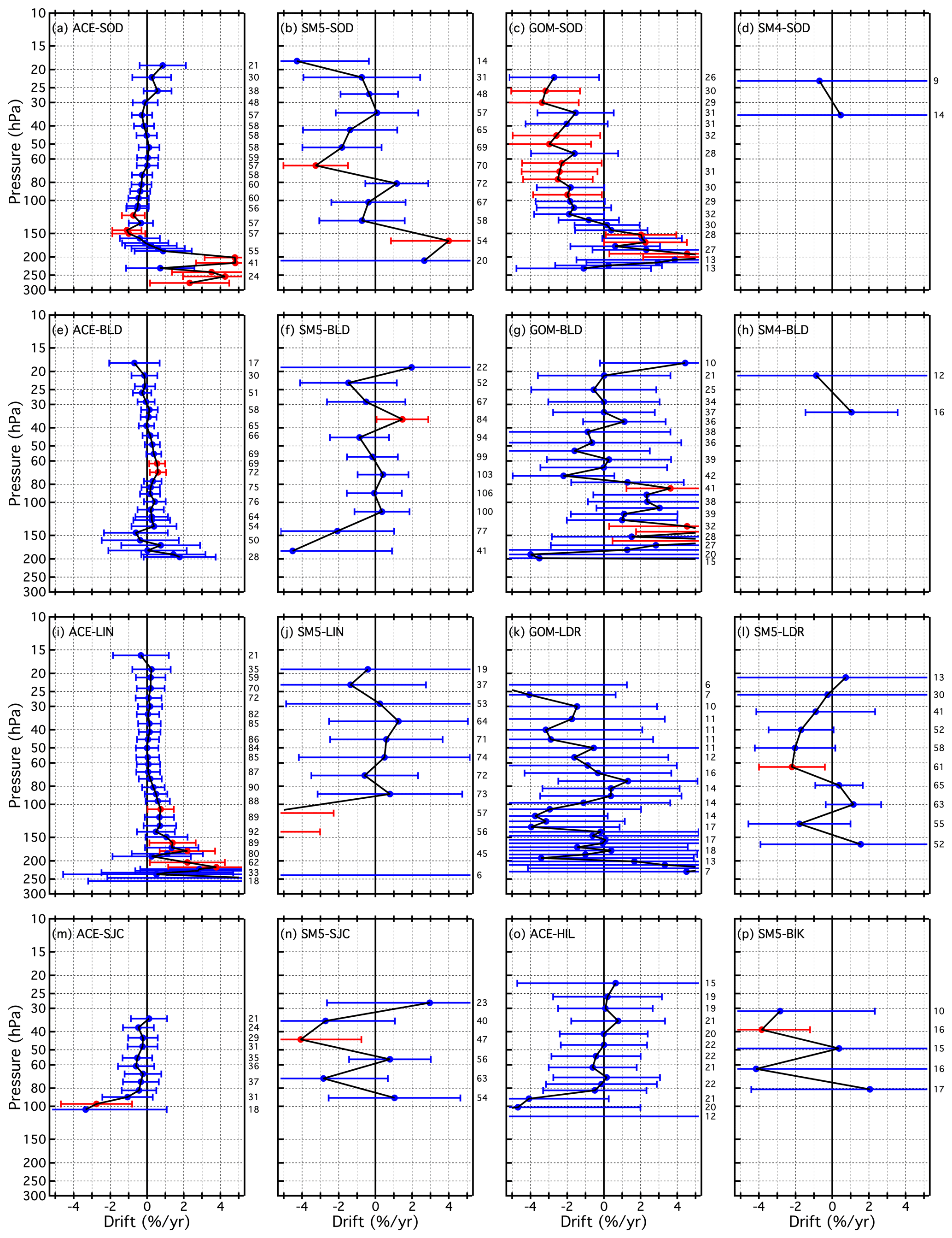
Figure B2Same as Fig. B1 for 16 additional SAT–FP pairings that include ACE, SM5, GOM, and SM4.
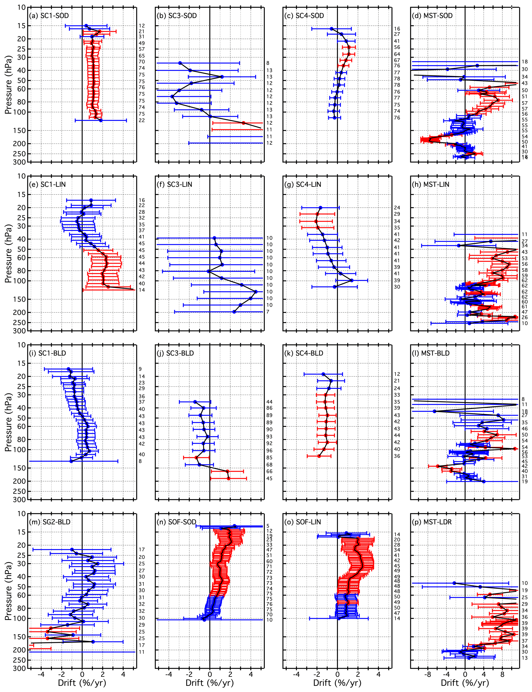
Figure B3Same as Fig. B1 for 16 additional SAT–FP pairings that include SC1, SC3, SC4, SG2, SOF, and MST. Note that the x-axis scale for the far right panels is expanded to better show the drifts.
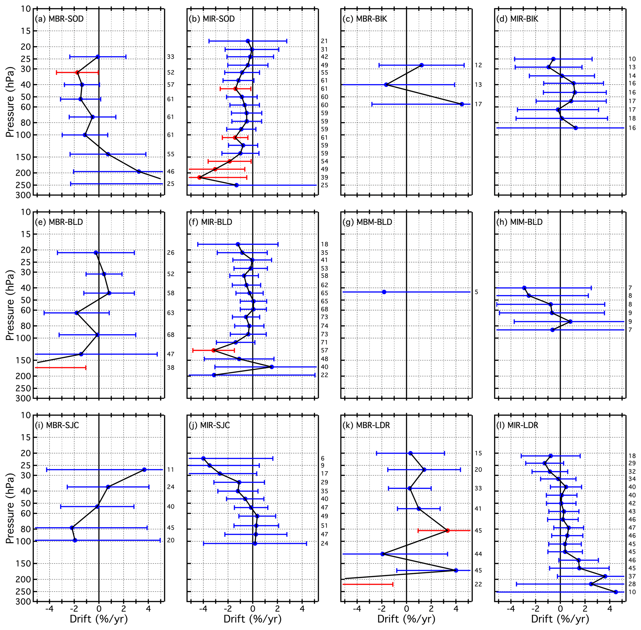
Figure B4Same as Fig. B1 for 12 additional SAT–FP pairings that include MBR, MIR, MBM, and MIM.
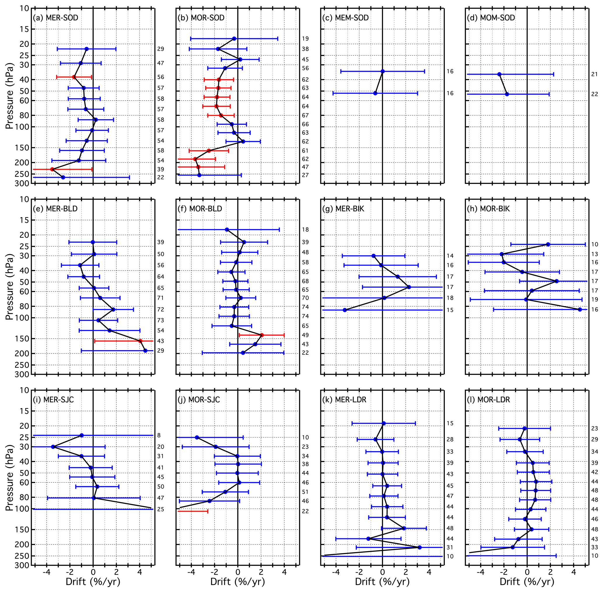
B2 Drifts per SAT data set
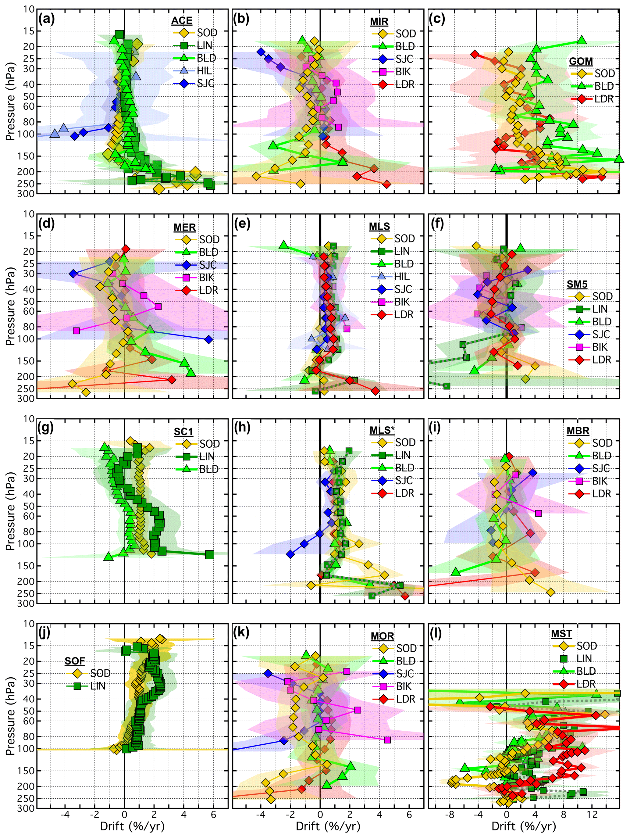
Figure B6Vertical profiles of drifts in SAT–FP differences. Each panel displays the drifts for one SAT (ACE, MIR, GOM, MER, MLS, SM5, SC1, MLS∗, MBR, SOF, MOR, and MST) paired with 1–7 different FP sites. Drifts over each FP site (connected coloured markers) are presented with their 95 % confidential intervals (coloured-matched shading). Shading that does not cross the black vertical line at 0 % drift indicates drifts that are statistically significant. Note that the x-axis scale for the panels in the far right column is expanded to show the drifts with greater clarity.
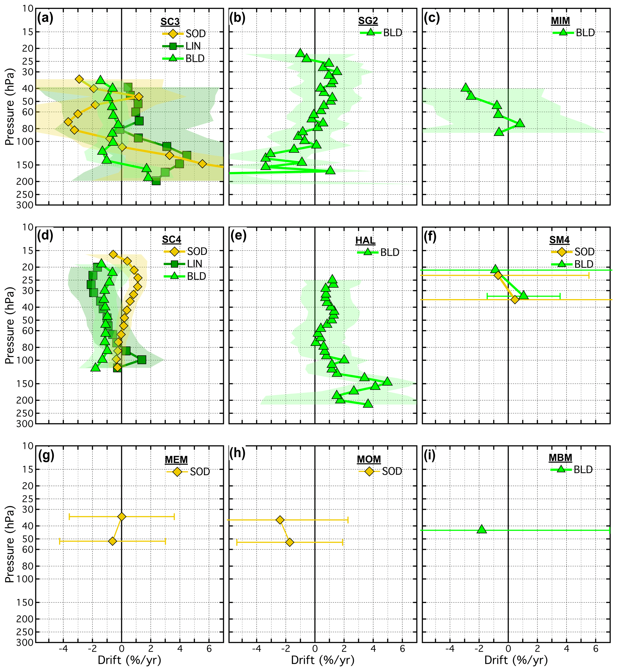
B3 Drifts per FP data set, ordered by latitude
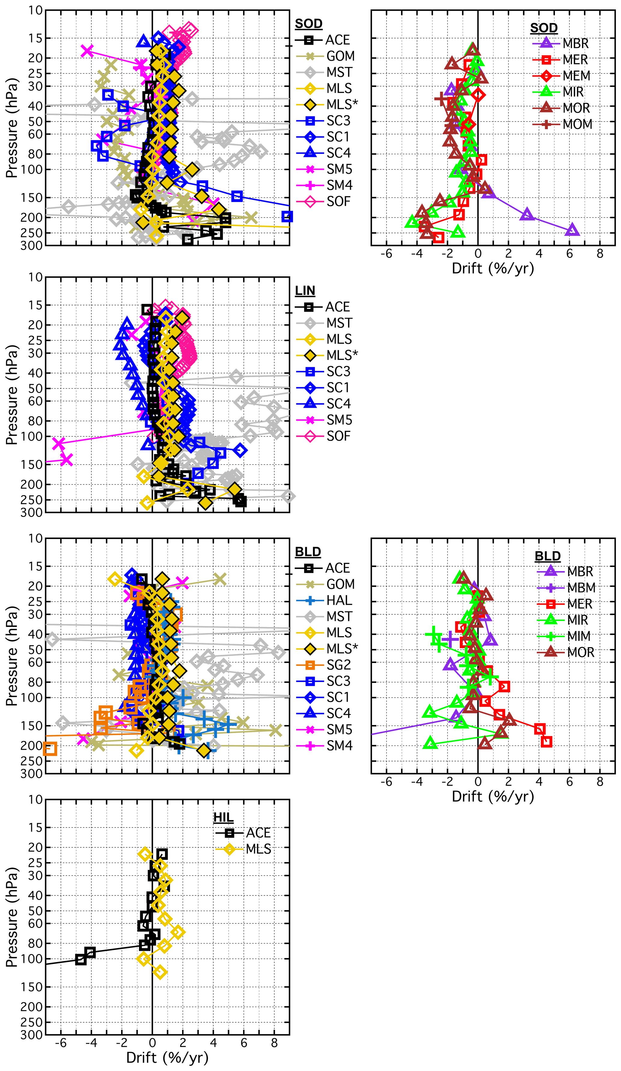
Figure B8Vertical profiles of drifts in SAT–FP differences. Each panel displays the drifts for the multiple SATs paired with each FP site (SOD, LIN, BLD, and HIL). Profiles for non-MIPAS SATs appear in the left column and for MIPAS SATs appear in the right column. For LIN and HIL there were no pairings with MIPAS SATs.
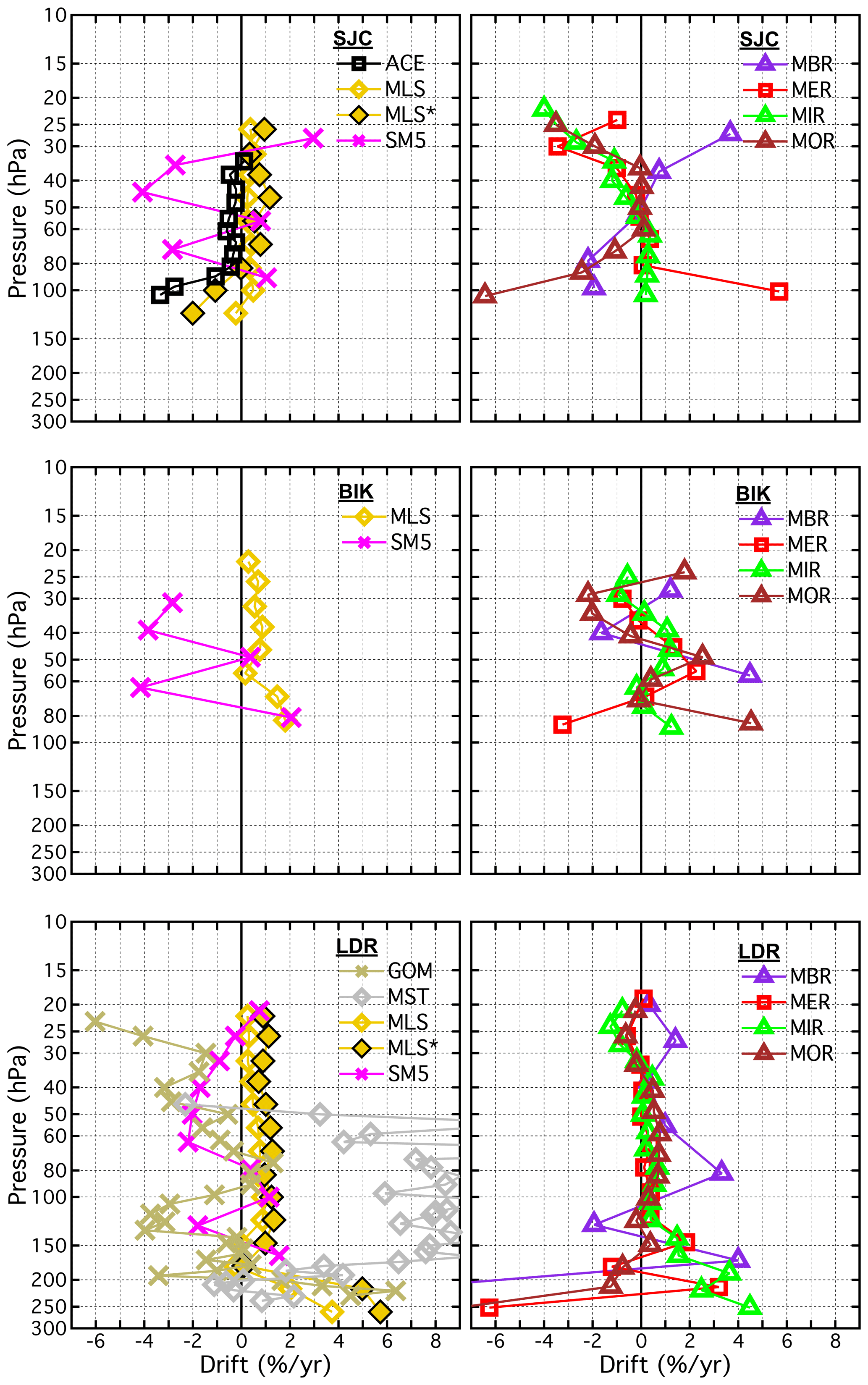
The satellite data records used in this study are publicly available from https://doi.org/10.5445/IR/1000093970 (Laeng, 2019).
The supplement related to this article is available online at: https://doi.org/10.5194/amt-16-4589-2023-supplement.
This study was conceived by the SPARC WAVAS-II core members JCG, DFH, FK, MK, SL, GEN, WGR, KHR, GPS, and KAW and led by DFH and MK. TvC contributed to the methodology of the bias part. GPS contributed text to the bias part and to the conclusions. The frost-point data were provided by DFH and HV. Expert advice on the usage and handling of satellite data was provided by JA, FA, JLB, LB, KB, JPB, RD, BMD, PE, MGC, JCG, MH, YK, MK, SL, DM, SN, PR, WGR, AR, CES, GPS, TS, TvC, KAW, and KW. All authors contributed to discussions and the conclusions.
At least one of the (co-)authors is a member of the editorial board of Atmospheric Measurement Techniques. The peer-review process was guided by an independent editor, and the authors also have no other competing interests to declare.
Publisher’s note: Copernicus Publications remains neutral with regard to jurisdictional claims in published maps and institutional affiliations.
This article is part of the special issue “Water vapour in the upper troposphere and middle atmosphere: a WCRP/SPARC satellite data quality assessment including biases, variability, and drifts (ACP/AMT/ESSD inter-journal SI)”. It does not belong to a conference.
Dale Hurst thanks the NASA Upper Atmosphere Composition Observations programme for continued financial support. The Atmospheric Chemistry Experiment (ACE), also known as SCISAT, is a Canadian-led mission mainly supported by the Canadian Space Agency and the Natural Sciences and Engineering Research Council of Canada. We appreciate the HALOE Science Team and the many members of the HALOE project for producing and characterizing the high-quality HALOE data set. We would like to thank the European Space Agency for making the MIPAS level-1b data set available and providing SCIAMACHY spectral data. The Oxford MIPAS data were provided by A. Dudhia. MLS data were obtained from the NASA Goddard Earth Sciences and Information Center. Work at the Jet Propulsion Laboratory, California Institute of Technology, was done under contract with the National Aeronautics and Space Administration. Thanks to Hauke Schmidt for providing the HAMMONIA data used for the convolution of higher vertically resolved data sets. We want to express our gratitude to SPARC and WCRP (World Climate Research Programme) for their guidance, sponsorship, and support of the WAVAS-II programme.
Stefan Lossow was funded by the Stratospheric Change and its Role for Climate
Prediction (SHARP) (grant no. STI 210/9-2).
The article processing charges for this open-access publication were covered by the Karlsruhe Institute of Technology (KIT).
This paper was edited by Sandip Dhomse and reviewed by Hugh C. Pumphrey and Xin Zhou.
Barrett, E. W., Herndon Jr., L. R., and Carter, H. J.: Some Measurements of the Distribution of Water Vapor in the Stratosphere1, Tellus, 2, 302–311, https://doi.org/10.3402/tellusa.v2i4.8602, 1950. a
Blunier, T., Chappellaz, J. A., Schwander, J., Barnola, J. M., Desperts, T., Stauffer, B., and Raynaud, D.: Atmospheric methane, record from a Greenland Ice Core over the last 1000 year, Geophys. Res. Lett., 20, 2219–2222, https://doi.org/10.1029/93GL02414, 1993. a
Brewer, A. W.: Evidence for a world circulation provided by the measurements of helium and water vapour distribution in the stratosphere, Q. J. Roy. Meteorol. Soc., 75, 351–363, https://doi.org/10.1002/qj.49707532603, 1949. a
Brinkop, S., Dameris, M., Jöckel, P., Garny, H., Lossow, S., and Stiller, G.: The millennium water vapour drop in chemistry–climate model simulations, Atmos. Chem. Phys., 16, 8125–8140, https://doi.org/10.5194/acp-16-8125-2016, 2016. a
Dessler, A. E., Schoeberl, M. R., Wang, T., Davis, S., and Rosenlof, K. H.: Stratospheric water vapor feedback, P. Natl. Acad. Sci. USA, 110, 18087–18091, https://doi.org/10.1073/pnas.1310344110, 2013. a
Dessler, A. E., Schoeberl, M. R., Wang, T., Davis, S. M., Rosenlof, K. H., and Vernier, J.: Variations of stratospheric water vapor over the past three decades, J. Geophys. Res., 119, 12588–12598, https://doi.org/10.1002/2014JD021712, 2014. a
Dessler, A. E., Ye, H., Wang, T., Schoeberl, M. R., Oman, L. D., Douglass, A. R., Butler, A. H., Rosenlof, K. H., Davis, S. M., and Portmann, R. W.: Transport of ice into the stratosphere and the humidification of the stratosphere over the 2st century, Geophys. Res. Lett., 43, 2323–2329, https://doi.org/10.1002/2016GL067991, 2016. a
Fueglistaler, S. and Haynes, P. H.: Control of interannual and longer–term variability of stratospheric water vapor, J. Geophys. Res., 110, D24108, https://doi.org/10.1029/2005JD006019, 2005. a, b
Gettelman, A., Birner, T., Eyring, V., Akiyoshi, H., Bekki, S., Brühl, C., Dameris, M., Kinnison, D. E., Lefevre, F., Lott, F., Mancini, E., Pitari, G., Plummer, D. A., Rozanov, E., Shibata, K., Stenke, A., Struthers, H., and Tian, W.: The Tropical Tropopause Layer 1960–2100, Atmos. Chem. Phys., 9, 1621–1637, https://doi.org/10.5194/acp-9-1621-2009, 2009. a
Gettelman, A., Hegglin, M. I., Son, S.-W., Kim, J., Fujiwara, M., Birner, T., Kremser, S., Rex, M., Añel, J. A., Akiyoshi, H., Austin, J., Bekki, S., Braesike, P., Brühl, C., Butchart, N., Chipperfield, M., Dameris, M., Dhomse, S., Garny, H., Hardiman, S. C., Jöckel, P., Kinnison, D. E., Lamarque, J. F., Mancini, E., Marchand, M., Michou, M., Morgenstern, O., Pawson, S., Pitari, G., Plummer, D., Pyle, J. A., Rozanov, E., Scinocca, J., Shepherd, T. G., Shibata, K., Smale, D., Teyssèdre, H., and Tian, W.: Multimodel assessment of the upper troposphere and lower stratosphere: Tropics and global trends, J. Geophys. Res.-Atmos., 115, D00M08, https://doi.org/10.1029/2009JD013638, 2010. a
Hall, E. G., Jordan, A. F., Hurst, D. F., Oltmans, S. J., Vömel, H., Kühnreich, B., and Ebert, V.: Advancements, measurement uncertainties, and recent comparisons of the NOAA frost point hygrometer, Atmos. Meas. Tech., 9, 4295–4310, https://doi.org/10.5194/amt-9-4295-2016, 2016. a, b, c
Hegglin, M. I., Plummer, D. A., Shepherd, T. G., Scinocca, J. F., Anderson, J., Froidevaux, L., Funke, B., Hurst, D., Rozanov, A., Urban, J., von Clarmann, T., Walker, K. A., Wang, H. J., Tegtmeier, S., and Weigel, K.: Vertical structure of stratospheric water vapour trends derived from merged satellite data, Nat. Geosci., 7, 768–776, https://doi.org/10.1038/ngeo2236, 2014. a
Hu, D.-Z., Han, Y.-Y., Sang, W.-J., and Xie, F.: Trends of Lower- to Mid-Stratospheric Water Vapor Simulated in Chemistr y-Climate Models, Atmos. Ocean. Sci. Lett., 8, 57–62, https://doi.org/10.3878/AOSL20140088, 2015. a
Hurst, D. F., Hall, E. G., Jordan, A. F., Miloshevich, L. M., Whiteman, D. N., Leblanc, T., Walsh, D., Vömel, H., and Oltmans, S. J.: Comparisons of temperature, pressure and humidity measurements by balloon-borne radiosondes and frost point hygrometers during MOHAVE-2009, Atmos. Meas. Tech., 4, 2777–2793, https://doi.org/10.5194/amt-4-2777-2011, 2011a. a
Hurst, D. F., Oltmans, S. J., Vömel, H., Rosenlof, K. H., Davis, S. M., Ray, E. A., Hall, E. G., and Jordan, A. F.: Stratospheric water vapor trends over Boulder, Colorado: Analysis of the 30 year Boulder record, J. Geophys. Res., 116, D02306, https://doi.org/10.1029/2010JD015065, 2011b. a, b
Hurst, D. F., Lambert, A., Read, W. G., Davis, S. M., Rosenlof, K. H., Hall, E. G., Jordan, A. F., and Oltmans, S. J.: Validation of Aura Microwave Limb Sounder stratospheric water vapor measurements by the NOAA frost point hygrometer, J. Geophys. Res., 119, 1612–1625, https://doi.org/10.1002/2013JD020757, 2014. a
Hurst, D. F., Read, W. G., Vömel, H., Selkirk, H. B., Rosenlof, K. H., Davis, S. M., Hall, E. G., Jordan, A. F., and Oltmans, S. J.: Recent divergences in stratospheric water vapor measurements by frost point hygrometers and the Aura Microwave Limb Sounder, Atmos. Meas. Tech., 9, 4447–4457, https://doi.org/10.5194/amt-9-4447-2016, 2016. a, b
Inai, Y., Shiotani, M., Fujiwara, M., Hasebe, F., and Vömel, H.: Altitude misestimation caused by the Vaisala RS80 pressure bias and its impact on meteorological profiles, Atmos. Meas. Tech., 8, 4043–4054, https://doi.org/10.5194/amt-8-4043-2015, 2015. a
Laeng, A.: Institut für Meteorologie und Klimaforschung – Atmosphärische Spurenstoffe und Fernerkundung (IMK-ASF), Water vapour profiles from WAVAS SAtellite component in HARmonized format (WAVAS_SAHAR), Forschungsdaten [data set], https://doi.org/10.5445/IR/1000093970, 2019. a
Kiehl, J. T. and Trenberth, K. E.: Earth's Annual Global Mean Energy Budget, B. Am. Meteorol. Soc., 78, 197–208, 1997. a
Kley, D., Smit, H. G. J., Vömel, H., Grassl, H., Ramanathan, V., Crutzen, P. J., Williams, S., Meywerk, J., and Oltmans, S. J.: Tropospheric water‐vapour and ozone cross‐sections in a zonal plane over the central equatorial Pacific Ocean, Q. J. Roy. Meteorol. Soc., 123, 2009–2040, 1997. a
Kley, D., Russell III, J. M., and Phillips, C. (Eds.): Stratospheric Processes and their Role in Climate (SPARC) – Assessment of upper tropospheric and stratospheric water vapour, WCRP No. 113, WMO/TD – No. 1043, SPARC Report No.2, WMO/ICSU/IOC, Paris, 2000. a, b
Lelieveld, J., Crutzen, P. J., and Dentener, F. J.: Changing concentration, lifetime and climate forcing of atmospheric methane, Tellus B, 50, 128–150, https://doi.org/10.1034/j.1600-0889.1998.t01-1-00002.x, 1998. a
le Texier, H., Solomon, S., and Garcia, R. R.: The role of molecular hydrogen and methane oxidation in the water vapour budget of the stratosphere, Q. J. Roy. Meteorol. Soc., 114, 281–295, https://doi.org/10.1002/qj.49711448002, 1988. a
Lund, R. and Reeves, J.: Detection of Undocumented Changepoints: A Revision of the Two-Phase Regression Model, J. Climate, 15, 2547–2554, 2002. a
Nedoluha, G. E., Bevilacqua, R. M., Gomez, R. M., Hicks, B. C., Russell III, J. M., and Connor, B. J.: An evaluation of trends in middle atmospheric water vapor as measured by HALOE, WVMS, and POAM, J. Geophys. Res.-Atmos., 108, 4391, https://doi.org/10.1029/2002JD003332, 2003. a
Nedoluha, G. E., Kiefer, M., Lossow, S., Gomez, R. M., Kämpfer, N., Lainer, M., Forkman, P., Christensen, O. M., Oh, J. J., Hartogh, P., Anderson, J., Bramstedt, K., Dinelli, B. M., Garcia-Comas, M., Hervig, M., Murtagh, D., Raspollini, P., Read, W. G., Rosenlof, K., Stiller, G. P., and Walker, K. A.: The SPARC water vapor assessment II: intercomparison of satellite and ground-based microwave measurements, Atmos. Chem. Phys., 17, 14543–14558, https://doi.org/10.5194/acp-17-14543-2017, 2017. a
Oltmans, S. and Hofmann, D.: Increase in lower-stratospheric water vapour at a mid-latitude Northern Hemisphere site from 1981 to 1994, Nature, 374, 146–149, https://doi.org/10.1038/374146a0, 1995. a, b
Oltmans, S. J., Vömel, H., Hofmann, D. J., Rosenlof, K. H., and Kley, D.: The increase in stratospheric water vapor from balloonborne, frostpoint hygrometer measurements at Washington, D.C., and Boulder, Colorado, Geophys. Res. Lett., 27, 3453–3456, https://doi.org/10.1029/2000GL012133, 2000. a, b
Randel, W. and Park, M.: Diagnosing Observed Stratospheric Water Vapor Relationships to the Cold Point Tropical Tropopause, J. Geophys. Res.-Atmos., 124, 7018–7033, https://doi.org/10.1029/2019JD030648, 2019. a, b
Randel, W. J., Wu, F., Vömel, H., Nedoluha, G. E., and Forster, P.: Decreases in stratospheric water vapor after 2001: Links to changes in the tropical tropopause and the Brewer–Dobson circulation, J. Geophys. Res., 111, D12312, https://doi.org/10.1029/2005JD006744, 2006. a, b
Read, W. G., Stiller, G., Lossow, S., Kiefer, M., Khosrawi, F., Hurst, D., Vömel, H., Rosenlof, K., Dinelli, B. M., Raspollini, P., Nedoluha, G. E., Gille, J. C., Kasai, Y., Eriksson, P., Sioris, C. E., Walker, K. A., Weigel, K., Burrows, J. P., and Rozanov, A.: The SPARC Water Vapor Assessment II: assessment of satellite measurements of upper tropospheric humidity, Atmos. Meas. Tech., 15, 3377–3400, https://doi.org/10.5194/amt-15-3377-2022, 2022. a, b, c
Riese, M., Ploeger, F., Rap, A., Vogel, B., Konopka, P., Dameris, M., and Forster, P.: Impact of uncertainties of atmospheric mixing on simulated UTLS composition and related radiative effects, J. Geophys. Res., 117, D16305, https://doi.org/10.1029/2012JD017751, 2012. a
Rodgers, C. D.: Inverse Methods for Atmospheric Sounding: Theory and Practice, Vol. 2 of Series on Atmospheric, Oceanic and Planetary Physics, edited by: Taylor, F. W., World Scientific, Singapore, New Jersey, London, Hong Kong, https://doi.org/10.1142/3171, 2000. a
Rollins, A. W., Thornberry, T. D., Gao, R. S., Smith, J. B., Sayres, D. S., Sargent, M. R., Schiller, C., Krämer, M., Spelten, N., Hurst, D. F., Jordan, A. F., Hall, E. G., Vömel, H., Diskin, G. S., Podolske, J. R., Christensen, L. E., Rosenlof, K. H., Jensen, E. J., and Fahey, D. W.: Evaluation of UT/LS hygrometer accuracy by intercomparison during the NASA MACPEX mission, J. Geophys. Res.-Atmos., 119, 1915–1935, https://doi.org/10.1002/2013JD020817, 2014. a
Rosenlof, K. H., Oltmans, S. J., Kley, D., Russell III, J. M., Chiou, E.-W., Chu, W. P., Johnson, D. G., Kelly, K. K., Michelsen, H. A., Nedoluha, G. E., Remsberg, E. E., Toon, G. C., and McCormick, M. P.: Stratospheric water vapor increases over the past half-century, Geophys. Res. Lett., 28, 1195–1198, https://doi.org/10.1029/2000GL012502, 2001. a
Scherer, M., Vömel, H., Fueglistaler, S., Oltmans, S. J., and Staehelin, J.: Trends and variability of midlatitude stratospheric water vapour deduced from the re-evaluated Boulder balloon series and HALOE, Atmos. Chem. Phys., 8, 1391–1402, https://doi.org/10.5194/acp-8-1391-2008, 2008. a, b
Schmidt, H., Brasseur, G. P., Charron, M., Manzini, E., Giorgetta, M. A., Diehl, T., Fomichev, V. I., Kinnison, D., Marsch, D., and Walters, S.: The HAMMONIA Chemistry Climate Model: Sensitivity of the Mesopause Region to the 11-year solar cycle and CO2 doubling, J. Climate, 19, 3903–3931, https://doi.org/10.1175/JCLI3829.1, 2006. a
Solomon, S., Rosenlof, K. H., Portmann, R. W., Daniel, J. S., Davis, S. M., Sanford, T. J., and Plattner, G.-K.: Contributions of Stratospheric Water Vapor to Decadal Changes in the Rate of Global Warming, Science, 327, 1219–1223, https://doi.org/10.1126/science.1182488, 2010. a
Stauffer, R. M., Morris, G. A., Thompson, A. M., Joseph, E., Coetzee, G. J. R., and Nalli, N. R.: Propagation of radiosonde pressure sensor errors to ozonesonde measurements, Atmos. Meas. Tech., 7, 65–79, https://doi.org/10.5194/amt-7-65-2014, 2014. a
Stiller, G. P., Kiefer, M., Eckert, E., von Clarmann, T., Kellmann, S., García-Comas, M., Funke, B., Leblanc, T., Fetzer, E., Froidevaux, L., Gomez, M., Hall, E., Hurst, D., Jordan, A., Kämpfer, N., Lambert, A., McDermid, I. S., McGee, T., Miloshevich, L., Nedoluha, G., Read, W., Schneider, M., Schwartz, M., Straub, C., Toon, G., Twigg, L. W., Walker, K., and Whiteman, D. N.: Validation of MIPAS IMK/IAA temperature, water vapor, and ozone profiles with MOHAVE-2009 campaign measurements, Atmos. Meas. Tech., 5, 289–320, https://doi.org/10.5194/amt-5-289-2012, 2012. a
Vömel, H., Naebert, T., Dirksen, R., and Sommer, M.: An update on the uncertainties of water vapor measurements using cryogenic frost point hygrometers, Atmos. Meas. Tech., 9, 3755–3768, https://doi.org/10.5194/amt-9-3755-2016, 2016. a, b, c
Vömel, H., David, D. E., and Smith, K.: Accuracy of tropospheric and stratospheric water vapor measurements by the cryogenic frost point hygrometer: Instrumental details and observations, J. Geophys. Res., 112, D08305, https://doi.org/10.1029/2006JD007224, 2007a. a, b
Vömel, H., Yushkov, V., Khaykin, S., Korshunov, L., Kyro, E., and Kivi, R.: Intercomparison of stratospheric water vapor sensors: FLASH-b and NOAA/CMDL frost point hygrometer, J. Atmos. Ocean. Technol., 27, 941–952, https://doi.org/10.1175/JTECH2007.1, 2007b. a, b
Walker et al.: Overview: the SPARC water vapour assessment II, Atmos. Meas. Tech., to be submitted, 2023. a, b
World Meteorological Organization: Definition of the tropopause, Bulletin of the World Meteorological Organization, 6, 136–137, 1957. a
- Abstract
- Introduction
- Data and data handling
- Bias assessment from vertical profile comparisons
- Assessment of drifts in satellite–FP differences
- Summary and conclusions
- Appendix A: Bias-related plots
- Appendix B: Drift-related plots
- Data availability
- Author contributions
- Competing interests
- Disclaimer
- Special issue statement
- Acknowledgements
- Financial support
- Review statement
- References
- Supplement