the Creative Commons Attribution 4.0 License.
the Creative Commons Attribution 4.0 License.
 | 12 Oct 2023
A research product for tropospheric NO2 columns from Geostationary Environment Monitoring Spectrometer based on Peking University OMI NO2 algorithm
Yuhang Zhang
Jhoon Kim
Hanlim Lee
Junsung Park
Hyunkee Hong
Michel Van Roozendael
Francois Hendrick
Ting Wang
Pucai Wang
Yongjoo Choi
Yugo Kanaya
Jin Xu
Pinhua Xie
Sanbao Zhang
Shanshan Wang
Siyang Cheng
Xinghong Cheng
Jianzhong Ma
Thomas Wagner
Robert Spurr
Lulu Chen
Hao Kong
Mengyao Liu
Tropospheric vertical column densities (VCDs) of nitrogen dioxide (NO2) retrieved from sun-synchronous satellite instruments have provided abundant NO2 data for environmental studies, but such data are limited by retrieval uncertainties and insufficient temporal sampling (e.g., once a day). The Geostationary Environment Monitoring Spectrometer (GEMS) launched in February 2020 monitors NO2 at an unprecedented hourly resolution during the daytime. Here we present a research product for tropospheric NO2 VCDs, referred to as POMINO–GEMS (where POMINO is the Peking University OMI NO2 algorithm). We develop a hybrid retrieval method combining GEMS, TROPOMI (TROPOspheric Monitoring Instrument) and GEOS-CF (Global Earth Observing System Composition Forecast) data to generate hourly tropospheric NO2 slant column densities (SCDs). We then derive tropospheric NO2 air mass factors (AMFs) with explicit corrections for surface reflectance anisotropy and aerosol optical effects through parallelized pixel-by-pixel radiative transfer calculations. Prerequisite cloud parameters are retrieved with the O2–O2 algorithm by using ancillary parameters consistent with those used in NO2 AMF calculations.
The initial retrieval of POMINO–GEMS tropospheric NO2 VCDs for June–August 2021 exhibits strong hotspot signals over megacities and distinctive diurnal variations over polluted and clean areas. POMINO–GEMS NO2 VCDs agree with the POMINO–TROPOMI v1.2.2 product (R=0.98; NMB = 4.9 %) over East Asia, with slight differences associated with satellite viewing geometries and cloud and aerosol properties affecting the NO2 retrieval. POMINO–GEMS also shows good agreement with the following: OMNO2 (Ozone Monitoring Instrument (OMI) NO2 Standard Product) v4 (R=0.87; NMB = −16.8 %); and GOME-2 (Global Ozone Monitoring Experiment-2) GDP (GOME Data Processor) 4.8 (R=0.83; NMB = −1.5 %) NO2 products. POMINO–GEMS shows small biases against ground-based MAX-DOAS (multi-axis differential optical absorption spectroscopy) NO2 VCD data at nine sites (NMB = −11.1 %), with modest or high correlation in diurnal variation at six urban and suburban sites (R from 0.60 to 0.96). The spatiotemporal variation in POMINO–GEMS correlates well with mobile car MAX-DOAS measurements in the Three Rivers source region on the Tibetan Plateau (R=0.81). Surface NO2 concentrations estimated from POMINO–GEMS VCDs are consistent with measurements from the Ministry of Ecology and Environment of China for spatiotemporal variation (R=0.78; NMB = −26.3 %) and diurnal variation at all, urban, suburban and rural sites (R≥0.96). POMINO–GEMS data will be made freely available for users to study the spatiotemporal variations, sources and impacts of NO2.
- Article
(14096 KB) - Full-text XML
-
Supplement
(3896 KB) - BibTeX
- EndNote


Tropospheric nitrogen dioxide (NO2) is an important air pollutant. It threatens human health, and contributes to the formation of tropospheric ozone (O3) and nitrate aerosols (Crutzen, 1970; Shindell et al., 2009; Hoek et al., 2013; Chen et al., 2022). Satellite instruments provide observations of tropospheric NO2 on a global scale, and they have been extensively used to estimate emissions of nitrogen oxides (NOx = NO + NO2; Lin and Mcelroy, 2011; Beirle et al., 2011; Gu et al., 2014; Kong et al., 2022), surface NO2 concentrations (Wei et al., 2022; Cooper et al., 2022), trends and variabilities (Richter et al., 2005; Cui et al., 2016; Krotkov et al., 2016; van der A et al., 2017) and impacts on human health and environment (Chen et al., 2021).
To date, most spaceborne instruments for NO2 measurements, including the Global Ozone Monitoring Experiment (GOME; Burrows, 1999), the Ozone Monitoring Instrument (OMI; Levelt et al., 2006), the Global Ozone Monitoring Experiment 2 (GOME-2; Callies et al., 2000) and the TROPOspheric Monitoring Instrument (TROPOMI; Veefkind et al., 2012), are mounted on sun-synchronous low Earth orbit (LEO) satellites. These instruments passively measure backscattered radiance from the Earth's atmosphere, and measurements at each ground location are done 1–2 times a day. The Geostationary Environment Monitoring Spectrometer (GEMS), on board the Geostationary Korea Multi-Purpose Satellite-2B (GK-2B), was successfully launched in February 2020. The instrument provides measurements of NO2 and other pollutants in the daytime on an hourly basis (Kim et al., 2020). It complements LEO satellite observations by providing a more comprehensive picture of the daytime evolution of NO2.
There are three successive stages in the retrieval of tropospheric NO2 vertical column densities (VCDs) in the UV-Vis (visible) range based on satellite observations. The first step is to retrieve total NO2 slant column densities (SCDs) with spectral fitting techniques, such as the differential optical absorption spectroscopy (DOAS). The SCD represents the abundance of NO2 along the effective light path from the Sun through the atmosphere to the satellite instrument. Next, the contributions from stratospheric NO2 to the total SCDs are removed in order to obtain tropospheric SCDs. Finally, the tropospheric SCDs are converted to VCDs using calculated air mass factors (AMFs). The AMF calculations are highly sensitive to the observation geometry, cloud parameters, aerosols, surface conditions and the shape of the NO2 vertical distribution. Over polluted areas, errors in the retrieved tropospheric NO2 VCDs are dominated by the uncertainties in AMF calculations (Boersma et al., 2004; Lorente et al., 2016) associated with aerosol optical effects, surface reflectance and a priori NO2 vertical profiles (Zhou et al., 2010; Lin et al., 2014, 2015; Vasilkov et al., 2016, 2021; Lorente et al., 2018; Liu et al., 2019, 2020).
The official GEMS retrieval algorithm for tropospheric NO2 VCDs is developed by Park et al. (2020). The total NO2 SCDs are retrieved using the DOAS technique. They are then converted to total NO2 VCDs by using a precomputed lookup table of box AMFs, based on the linearized pseudo-spherical scalar and vector discrete ordinate radiative transfer code (VLIDORT) version 2.6. Finally, stratosphere–troposphere separation (STS) is performed to derive tropospheric NO2. Validation results have shown the overall capability of the official GEMS NO2 algorithm (Kim et al., 2023), but several problems are also reported, such as overestimation of total NO2 SCDs and tropospheric NO2 VCDs, and some degree of striping in NO2 retrieval data.
In this study, we present a research product which we name POMINO–GEMS. This product is built upon our Peking University OMI NO2 (POMINO) algorithm, which focuses on the tropospheric AMF calculations and has been applied to OMI and TROPOMI (Lin et al., 2014, 2015; Liu et al., 2019, 2020; Zhang et al., 2022). Here we extend the AMF calculation by constructing a hybrid method to estimate tropospheric SCDs for GEMS. The hybrid method makes use of the total SCDs from the official GEMS product, total SCDs and stratospheric VCDs from the official TROPOMI product and hourly stratospheric VCD data from the NASA Global Earth Observing System Composition Forecast (GEOS-CF) v1 product. We validate our initial set of retrieval results for tropospheric NO2 VCDs in June, July and August (JJA) 2021, by using independent data of tropospheric NO2 from the POMINO–TROPOMI v1.2.2, OMNO2 (OMI NO2 Standard Product) v4 and GOME-2 GDP (GOME Data Processor) 4.8 products, ground-based and mobile car MAX-DOAS (multi-axis differential optical absorption spectroscopy) measurements and surface concentration observations from the Ministry of Ecology and Environment (MEE) of China. We provide a simplified estimate of retrieval errors in the end.
2.1 Construction of POMINO–GEMS retrieval algorithm
Figure 1 shows the flow chart of the POMINO–GEMS retrieval algorithm. There are two essential steps. The first is to calculate tropospheric NO2 SCDs on an hourly basis, through the fusion of total SCDs from the official GEMS v1.0 L2 NO2 product, total SCDs and stratospheric VCDs from the TROPOMI Product Algorithm Laboratory (PAL) v2.3.1 L2 NO2 product and diurnal variations in the stratospheric NO2 from the GEOS-CF v1 product. We then calculate tropospheric NO2 AMFs to convert SCDs to VCDs.
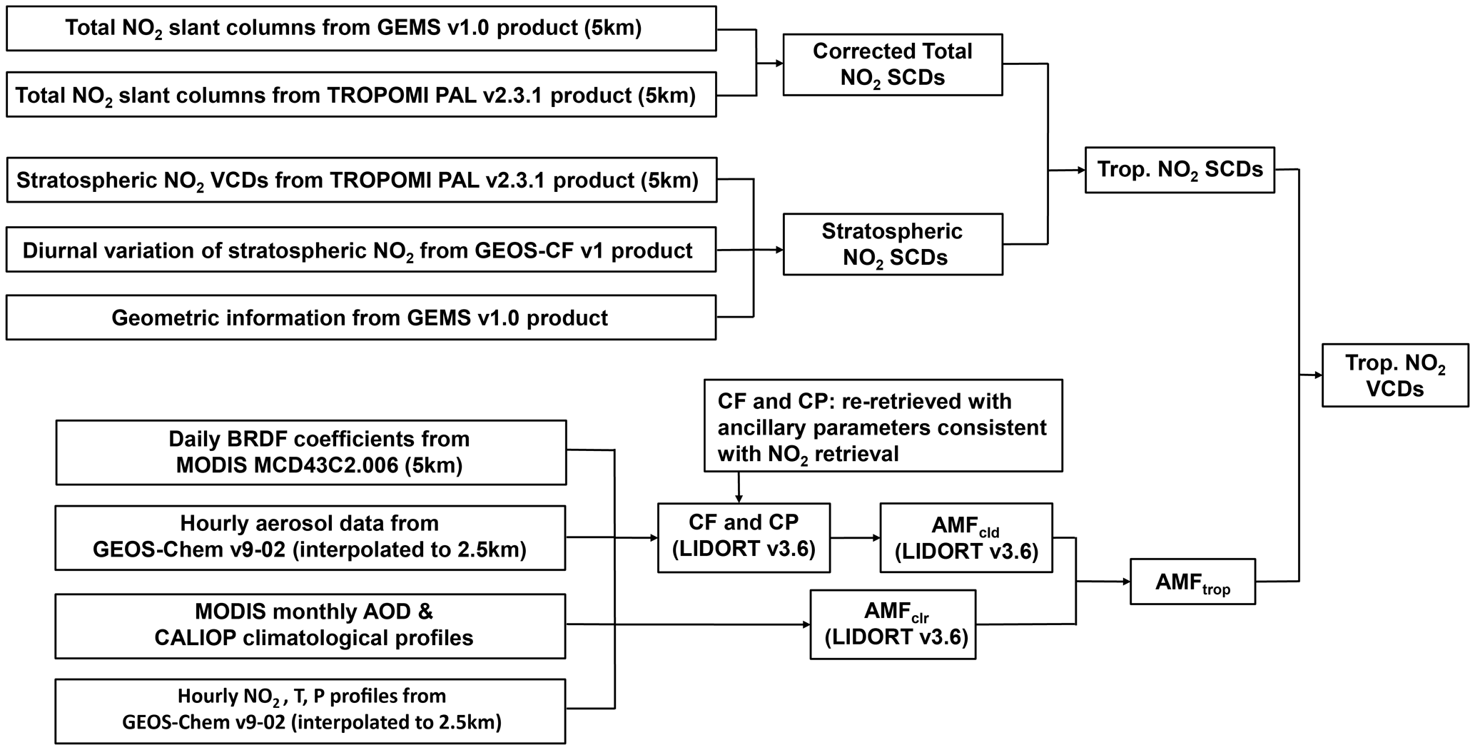
Figure 1Flow chart of the POMINO–GEMS retrieval algorithm. The numbers in the boxes, such as 5 km, refer to the horizontal resolutions.
2.1.1 GEMS NO2 and cloud data
The GEMS instrument is on board the GK-2B satellite located at 128.2∘ E over the Equator (Kim et al., 2020). The spectral wavelength range of GEMS is 300–500 nm, which covers the main absorption spectra of aerosols and trace gases. The nominal spatial resolution is typically 7 km × 8 km for gases and 3.5 km × 8 km for aerosols in the eastern and central scan domains; however, the north–south spatial resolution can exceed 25 km in the western side. The whole field of view (FOV) covers about 20 Asian countries within latitudes 45∘ N to 5∘ S and longitudes 80 to 152∘ E. Given the variation in the solar zenith angle (SZA), there are four scan scenarios moving from east to west, including half east (HE), half Korea (HK), full central (FC) and full west (FW). It takes 30 min (for example, 00:45–01:15 UTC) for GEMS to scan its full coverage during each scenario, and another 30 min to transmit data to the ground data center. The number of hourly GEMS observations per day varies from 6 in winter to 10 in summer, corresponding to the annual movement of subsolar points relative to the Earth.
We take hourly total (stratospheric plus tropospheric) NO2 SCDs from the official GEMS v1.0 L2 NO2 product and convert them to 0.05∘ × 0.05∘ gridded data by means of an area-weighted oversampling technique. The value of each grid cell is the mean value of pixel-based GEMS observations weighted by the ratio of the overlap area of each pixel to the area of grid cell. We also use continuum reflectance data (i.e., spectrally smooth reflectance from molecular and aerosol extinction, as well as surface reflectance effects) and O2–O2 SCDs from the official GEMS v1.0 L2 cloud product to re-calculate cloud parameters as a prerequisite for tropospheric NO2 AMF calculations. Details of the GEMS retrievals can be found in the Algorithm Theoretical Basis Document (ATBD; Park et al., 2020).
2.1.2 TROPOMI, OMI and GOME-2 NO2 data
Table S1 in the Supplement compares the basic information of GEMS with those of TROPOMI, OMI and GOME-2 instruments. In this study, TROPOMI data are used for the derivation of POMINO–GEMS NO2 VCDs, and data from all three LEO instruments are used for comparison with POMINO–GEMS.
We use total NO2 SCDs and stratospheric NO2 VCDs from the official TROPOMI PAL v2.3.1 L2 NO2 product and convert them to 0.05∘ × 0.05∘ gridded data, again using an area-weighted oversampling technique. Details of TROPOMI total SCD retrievals and stratospheric VCD calculations are given in the TROPOMI ATBD (Van Geffen et al., 2022a). The TROPOMI PAL product is reprocessed with TROPOMI NO2 data processor v2.3.1 for the period from 1 May 2018 to 14 November 2021; it will be replaced by the full mission reprocessing with a NO2 processor v2.4.0 in the future (Eskes et al., 2021). The most important improvement in this PAL product upon the previous OFFL (offline; non-time-critical data product) v1.3 is the replacement of the FRESCO (Fast Retrieval Scheme for Clouds from the Oxygen A band)-S algorithm with the FRESCO-wide cloud retrieval algorithm, which leads to higher, more reasonable cloud pressure (CP) estimates and substantial increases in tropospheric NO2 VCDs (by 20 %–50 %) over polluted regions like eastern China in winter (Eskes et al., 2021; Van Geffen et al., 2022b).
We use the POMINO–TROPOMI v1.2.2, OMNO2 v4 (Lamsal et al., 2021) and GOME-2 GDP 4.8 (Valks et al., 2019b) tropospheric NO2 VCD products to compare with POMINO–GEMS results. The previous POMINO–TROPOMI v1 data show higher accuracy in polluted situations and improved consistency with MAX-DOAS measurements when compared with the official TM5-MP-DOMINO (OFFLINE) product (Liu et al., 2020). POMINO–TROPOMI v1.2.2 improves upon v1 by (1) using tropospheric NO2 SCD and CP data from the updated TROPOMI PAL v2.3.1 NO2 product; (2) interpolating the daily NO2, pressure, temperature and aerosol vertical profiles from nested GEOS-Chem (v9-02) simulations into a horizontal grid of 2.5 km × 2.5 km for subsequent tropospheric AMF calculations; and (3) including several minor bug fixes.
We select valid satellite pixels following common practice. For the daily POMINO–TROPOMI v1.2.2 L2 NO2 product, we exclude pixels with SZA or viewing zenith angle (VZA) greater than 80∘, high albedos caused by ice or snow on the ground, quality flag values (from the TROPOMI PAL v2.3.1 product) less than 0.5 or a cloud radiance fraction (CRF) greater than 50 %; then, we map the valid data to a 0.05∘ × 0.05∘ grid. For the daily OMNO2 v4 L2 NO2 product, we exclude pixels with SZA or VZA greater than 80∘, with scene Lambertian equivalent reflectivity (LER) greater than 0.3, affected by row anomaly (XTrackQualityFlags is not zero), marked without quality assurance (vcdQualityFlag is not an even integer) or with CRF greater than 50 %; then, we map the valid data to a 0.25∘ × 0.25∘ grid. For the daily GOME-2 GDP 4.8 L2 NO2 product, we exclude pixels with latitude greater than 70∘, SZA greater than 80∘, failed retrieval (NO2Tropo_Flag is set to 1 or 2) or with CRF greater than 50 % and then map the valid data to a 0.5∘ × 0.5∘ grid.
2.1.3 GEOS-CF stratospheric NO2 data
The NASA GEOS-CF system combines the Global Earth Observing System (GEOS) weather analysis and forecasting system with GEOS-Chem v12.0.1 chemistry module (http://geoschem.org, last access: 16 July 2023) to provide near-real-time estimates of atmospheric compositions with daily 5 d forecasts. Detailed information of the model, including chemistry, emissions and deposition, and an evaluation of the GEOS-CF tropospheric simulation and forecast skill are presented in Keller et al. (2021). In particular, the GEOS-Chem v12.0.1 chemistry scheme includes online stratospheric chemistry that is fully coupled with tropospheric chemistry through the Unified tropospheric–stratospheric Chemistry eXtension (UCX) mechanism (Eastham et al., 2014). The GEOS-CF stratospheric results are consistent with satellite observations, although with notable underestimations of NOx and HNO3 in the polar regions (Knowland et al., 2022).
The GEOS-CF outputs have a horizontal resolution of 0.25∘ × 0.25∘ and a temporal resolution of 1 h for NO2 and other ancillary data used here (Knowland et al., 2020). We convert the instantaneous stratospheric NO2 volume mixing ratio in dry air at each hour (e.g., 00:00 UTC) into 0.05∘ × 0.05∘ gridded vertical column densities, based on estimated tropopause information in GEOS-CF v1. In Sect. 2.1.5, we first evaluate GEOS-CF v1 stratospheric NO2 VCDs with those of TROPOMI PAL v2.3.1 product and then calculate hourly stratospheric NO2 VCDs by combining GEOS-CF v1 data for each hour and TROPOMI PAL v2.3.1 stratospheric NO2 VCD data in the early afternoon.
2.1.4 Calculation of total NO2 SCDs
We use TROPOMI data to correct GEMS total NO2 SCDs, given the known issues in GEMS data. Specifics for the NO2 SCD retrieval of TROPOMI PAL v2.3.1 and GEMS v1.0 operational products are provided in Table S2.
Figure 2a and b show the spatial distribution of monthly mean total NO2 geometric column densities (GCDs, which are calculated as SCDs divided by geometric AMFs) in June 2021 from TROPOMI PAL v2.3.1 and GEMS v1.0, respectively. The horizontal resolution is 0.05∘ × 0.05∘. The GCDs are used to compare the two products after removing the effect of measurement geometry. Matching for each day between hourly GEMS observations and the TROPOMI data at the closest observation time is done to ensure temporal compatibility. The figures show that the spatial pattern of GEMS GCDs agrees well with that of TROPOMI, with high values over the North China Plain (NCP) and northwestern India, as well as major metropolitan clusters such as Seoul and the Yangtze River Delta (YRD). However, there are two systematic problems in GEMS GCDs. First, the GEMS GCD values are abnormally high over the northern and northwestern parts of GEMS FOV, especially over Mongolia, Qinghai, Inner Mongolia, Xinjiang and Tibet. Second, west–east stripes exist over the whole domain, similar to the spurious across-track variability issue for OMI. This stripe issue exists at all hours (Fig. S1 in the Supplement). It is likely associated with the specific scan modes of GEMS and the periodically occurring bad pixels, which is one of the remaining calibration issues (Boersma et al., 2011; Lee et al., 2023).
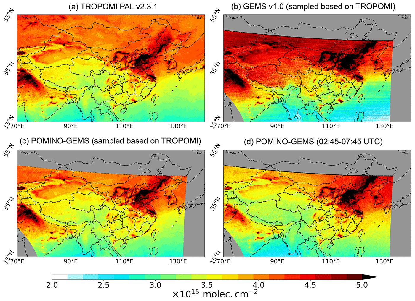
Figure 2Spatial distribution of monthly mean total NO2 GCDs on a 0.05∘ × 0.05∘ grid in June 2021. (a) The TROPOMI PAL v2.3.1 product. (b) The official GEMS v1.0 product that spatiotemporally matches with TROPOMI. (c) The corrected POMINO–GEMS product that spatiotemporally matches with TROPOMI. (d) The corrected POMINO–GEMS product averaged over 02:45–07:45 UTC. Note that the range of the color bar is 2.0–5.0 × 10¹⁵ . The regions in gray mean that there are no valid observations.
To correct the two issues in the GEMS official total NO2 SCD product, we combine GEMS and TROPOMI observations to obtain hourly 0.05∘ × 0.05∘ corrected total NO2 SCDs for each day, using Eqs. (1) and (2) as follows:
In Eqs. (1) and (2), index h represents the hour of GEMS observations on each day. hi the hour when both GEMS and TROPOMI have valid observations for the same grid cell, and n is the number of hi. The value of n is 1 or 2, depending on the overpass times of TROPOMI. There are two steps in the correction process. First, we calculate a geometry-independent correction map for each day, using total NO2 GCDs from GEMS and TROPOMI that match spatially and temporally (Eq. 1). We use the absolute difference instead of a scaling factor as a simple correction. We then apply the correction to the original GEMS total NO2 SCDs at each hour on the same day, with the diurnal variation in AMF associated with the measurement geometry accounted for (Eq. 2).
In Eq. (2), we implement a simple geometric correction (concerning SZAs and VZAs) for AMFs instead of using the actual AMFs; the latter could account for the differences in the relative azimuth angles and other factors. A specific derivation of this assumption is given in Sect. S1 in the Supplement. The correction is assumed to be acceptable, with an extra uncertainty introduced to the total NO2 SCDs, as will be further discussed in Sect. 3.5.
Figure 2c shows the monthly mean corrected POMINO–GEMS total NO2 GCDs in June 2021 after spatial and temporal matching with TROPOMI. The corrected GCD values in the northern GEMS FOV are much reduced when compared with those in the original GEMS data. Moreover, most stripe-like patterns are removed in the corrected GCDs. Figure 2d is similar to Fig. 2c but for GCDs averaged over 02:45–07:45 UTC in June 2021. Figure S3 further compares the original GEMS and POMINO–GEMS total NO2 GCDs at each hour in JJA 2021, showing similar improvements as well. The differences between Fig. 2c and d indicate the influence of different sampling hours combined with the daily correction map. Specifically, the correction value of each grid cell is calculated at the specific hour when both GEMS and TROPOMI have valid observations, but this value is applied to original GEMS SCDs at all hours.
Our correction method is done for each grid cell. We tested other correction methods by applying the same correction value to grid cells within a 20∘ × 20∘ domain, at the same latitude or at the same longitude. These alternative methods can reduce the high bias over the northern and northwestern GEMS FOV to various extents but cannot remove the stripes (not shown). We also note that our simple correction is a temporary solution before the aforementioned systematic problems in the official GEMS SCD retrieval are solved by improving spectral fitting. In Sect. 3.3 and 3.4, we compare the diurnal variations in the tropospheric NO2 VCDs, based on corrected and uncorrected GEMS SCDs.
2.1.5 Calculation of stratospheric and tropospheric NO2 SCDs
We construct a dataset of hourly stratospheric NO2 SCDs at 0.05∘ × 0.05∘ by using TROPOMI PAL v2.3.1 stratospheric NO2 VCDs, diurnal variation in the stratospheric NO2 VCDs provided by GEOS-CF v1 product and GEMS geometric AMFs.
Figure S4 shows the comparison results between GEOS-CF v1 and TROPOMI PAL v2.3.1 stratospheric NO2 VCDs in June 2021. Consistent spatial and temporal sampling is done. N is the total number of matched 0.05∘ × 0.05∘ grid cells. The stratospheric VCDs from both products vary in the range of 2–5 × 10¹⁵ , with a spatiotemporal correlation of 0.99, linear regression slope of 0.99 and normalized mean bias (NMB) of 0.02 %. This consistency provides confidence on the overall reliability of GEOS-CF stratospheric NO2 data.
First, we calculate stratospheric NO2 VCDs at a reference hour for each day using Eqs. (3) and (4), as follows:
Here, Eq. (3) defines the ratio of GEOS-CF stratospheric NO2 at hour h to that at the reference hour h0, which is chosen to be 01:00 UTC (Fig. S5). In Eq. (4), hi represents the observation time of every TROPOMI orbit that overlaps with GEMS FOV, and n is the number of hi for each grid cell.
Second, we use the ratio from a given time h to h0 and stratospheric NO2 VCDs at h0 to derive stratospheric NO2 VCDs at h for each day (Eq. 5).
Figure 3 shows the derived monthly mean stratospheric NO2 VCDs at each hour in June 2021 on a 0.05∘ × 0.05∘ grid. The abrupt decease in the stratospheric NO2 VCDs after sunrise is caused by resumed photochemical conversion of NO2 to NO (K.-F. Li et al., 2021). There is a strong meridional gradient of stratospheric NO2 in the daytime, with the higher values in the north associated with longer lifetimes. The stratospheric NO2 increase quasi-linearly during the daytime; the linear regression to the mean stratospheric NO2 VCDs over the whole domain from 01:45 to 07:45 UTC results in an increasing rate of (1.12 ± 0.03) × 1014 . This result is consistent with previous work showing quasi-linear growth in the daytime at rates of 0.5–2 × 10¹⁴ , which depend on latitude and season (K.-F. Li et al., 2021; Dirksen et al., 2011).
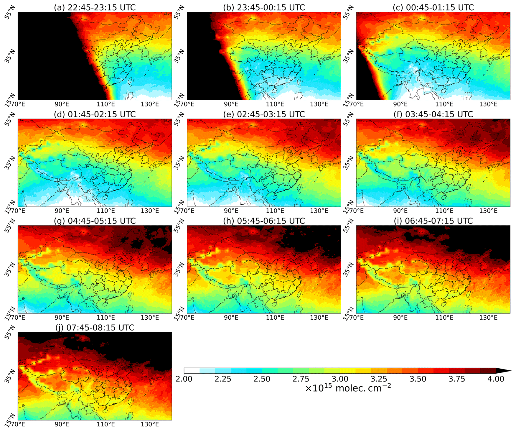
Figure 3Spatial distribution of POMINO–GEMS-derived monthly mean stratospheric NO2 VCDs at each hour on a 0.05∘ × 0.05∘ grid in June 2021. Note the range of the color bar is 2.0–4.0 × 10¹⁵ .
Finally, we use GEMS geometric AMFs to convert the stratospheric NO2 VCDs to SCDs at each hour and then subtract them from the total SCDs to obtain tropospheric SCDs (Eqs. 6 and 7). In the stratosphere, the geometric AMFs are essentially the same as the actual AMFs.
2.1.6 Calculation of tropospheric AMFs
Tropospheric NO2 AMF is dependent on the following three factors, as defined in Palmer et al. (2001): the viewing geometry, the scattering weights describing the sensitivity of the backscattered spectrum to the abundance of the absorber and the a priori NO2 vertical profile (Eq. 8).
In Eq. (8), AMFG is the geometric AMF and a function of SZA and VZA, w(z) the scattering weight at altitude z, S(z) the normalized vertical profile of NO2 number density, and zT the tropopause. Following Yang et al. (2023), we refer to as the scattering correction factor for discussion in Sect. 3.2. For tropospheric AMF calculations (Fig. 1), we use a parallelized AMFv6 package driven by LIDORT (LInearized Discrete Ordinate Radiative Transfer) version 3.6; this is similar to the one used in our previous POMINO products (Lin et al., 2014, 2015; Liu et al., 2019) but with modifications to adapt to the geostationary observing characteristics and high spatiotemporal resolution of GEMS. We take daily BRDF (bidirectional reflectance distribution function) coefficients with a horizontal resolution of 5 km from the MODIS MCD43C2.006 dataset (Lucht et al., 2000) to account for the anisotropy of surface reflectance over land and coastal ocean regions and OMLER v3 albedo over open ocean (Zhou et al., 2010; Lin et al., 2014; Liu et al., 2020). Hourly varying aerosol parameters, a priori NO2 profiles, temperature profiles and pressure profiles are interpolated from nested GEOS-Chem (v9-02) results to a horizontal resolution of 2.5 km, using the Piecewise Cubic Hermite Interpolating Polynomial (PCHIP) method. Furthermore, we deploy aerosol optical depth (AOD) observations from the MODIS/Aqua Collection 6.1 MYD04_L2 dataset to constrain model-simulated AOD on a monthly basis (Lin et al., 2014, 2015; Liu et al., 2019, 2020); we also use a self-constructed monthly climatological dataset of aerosol extinction profiles based on Cloud-Aerosol Lidar with Orthogonal Polarization (CALIOP) L2 data over 2007–2015 to constrain modeled aerosol vertical profiles on a monthly climatology basis (Liu et al., 2019). We re-retrieve cloud parameters based on O2–O2 SCDs and continuum reflectances from the official GEMS v1.0 cloud product, using ancillary parameters consistent with those used in NO2 AMF calculations. Instead of relying on a lookup table (LUT), we conduct pixel-by-pixel radiative transfer calculations with the parallelized AMFv6 package algorithm. The independent pixel approximation (IPA) is assumed for cloud-contaminated pixels, as in other algorithms. Finally, we use the AMF data to convert tropospheric NO2 SCDs to VCDs.
Invalid pixels in the POMINO–GEMS product are filtered based on the following criteria: we exclude pixels with SZA or VZA greater than 80∘ or with the ground covered by ice or snow. To minimize cloud contamination, we exclude pixels with CRF greater than 50 %.
2.2 Estimation of surface NO2 concentrations
In order to validate satellite NO2 products with surface concentration measurements from MEE, we convert tropospheric NO2 VCDs from satellite products on a 0.05∘ × 0.05∘ grid to surface NO2 mass concentrations using GEOS-Chem-simulated NO2 vertical profiles and the box heights of the lowest model layer (Eq. 9).
In Eq. (9), Csurf represents the estimated surface NO2 mass concentration (in µg m−3), the satellite tropospheric VCD (in ), RGC the GEOS-Chem-simulated hourly ratio of NO2 sub-column in the lowest layer to the total tropospheric column, M the NO2 molar mass (in µg mol−1), N the Avogadro constant and HGC the box height of the lowest layer (in m). The thickness of the lowest layer of GEOS-Chem (about 130 m) is too large for the layer average NO2 mass concentration to represent that near the ground (M. Liu et al., 2018); thus, the derived concentration is multiplied by a factor of 2 to roughly account for the vertical gradient from the height of the ground instrument to the center of the model layer. However, the constant correction factor of 2 neglects the diurnal variation in the NO2 vertical gradient, which is related to the diurnal variation in the planetary boundary layer (PBL) heights. This issue is discussed in detail in Sect. 3.4.
2.3 Ground-based MAX-DOAS measurements
We use ground-based MAX-DOAS NO2 measurements, together with POMINO–TROPOMI v1.2.2, OMNO2 v4 and GOME-2 GDP 4.8 NO2 products, to validate the POMINO–GEMS retrieval results. The types, geolocations and observation times of MAX-DOAS stations are summarized in Table S3, and the location of each site is shown in Fig. S6. Details of each site are described in Sect. S2. Kanaya et al. (2014) and Hendrick et al. (2014) have discussed the error in MAX-DOAS NO2 retrieval, where uncertainties from a priori aerosol and NO2 profiles are the largest source by 10 %–14 %, and the total retrieval uncertainty is typically 12 %–17 %.
To ensure sampling consistency in time, we average all valid MAX-DOAS measurements within each observation period of GEMS (i.e., 30 min) for hourly comparison and within ± 1.5 h of the TROPOMI, OMI and GOME-2 overpass times for daily comparison. Following the procedures in previous studies (Lin et al., 2014; Liu et al., 2020), we exclude all matched MAX-DOAS data for which the standard deviation exceeds 20 % of the mean value to minimize the influence of local events. To ensure sampling consistency in space, we select valid satellite pixels within 5 km of MAX-DOAS sites for POMINO–GEMS and POMINO–TROPOMI v1.2.2, 25 km for OMNO2 v4 and 50 km for GOME-2 GDP 4.8 and then conduct spatial averaging. The Grubbs statistical test, which is used to detect outliers in a univariate dataset assumed to exhibit normal distribution (Grubbs, 1950), is performed to exclude outliers in both MAX-DOAS and satellite data before comparison. Only one data pair from the Fudan University site is identified as an outlier and removed (Fig. S7), and we have 1348 matched hourly data pairs in total.
2.4 Mobile car MAX-DOAS measurements
We use tropospheric NO2 VCDs from mobile car MAX-DOAS measurements performed by the Chinese Academy of Meteorological Sciences (CAMS) in the Three Rivers source region in July 2021 (Cheng et al., 2023). The Three Rivers source region is on the northeastern Tibetan Plateau in western China, which is isolated from massive anthropogenic activities and hence a good place for observations of atmospheric compositions in the background atmosphere. The field campaign lasted from 18 to 30 July 2021 and included four closed-loop journeys, beginning from the meteorological bureau of the city of Xining (the capital of Qinghai Province) to the meteorological bureau of Dari county of the Guoluo Tibetan Autonomous Prefecture and then from the meteorological bureau of Dari county to the meteorological bureau of the Yushu Tibetan Autonomous Prefecture, and finally back to Xining city (Fig. S6). The spectral analysis of the measurement spectra in the fitting window of 400–434 nm was implemented with the DOAS method. A sequential Fraunhofer reference spectrum (FRS) is used to derive NO2 differential slant column densities (DSCDs), which are then converted to VCDs by adopting the geometric approximation method. The errors are estimated to be less than 20 % at high altitudes. More detailed descriptions of instrumentation, field campaign and data retrieval are in Cheng et al. (2023).
We average all valid mobile car MAX-DOAS measurements within each observation period of GEMS in each 0.05∘ × 0.05∘ grid cell to ensure spatiotemporal consistency. Over relatively clean areas with little human influence and biomass burning, such as the Three Rivers source region, a large portion of NO2 is located in the middle and upper troposphere, which is not accounted for in the mobile car data via such a DSCD-based retrieval method. Indeed, Cheng et al. (2023) showed that the official TROPOMI NO2 VCDs are higher than mobile car data by about 40 %. Considering that the diurnal variation in the middle and upper tropospheric NO2 is much smaller than that in the lower troposphere, we focus on the correlation of NO2 diurnal variation between POMINO–GEMS and mobile car MAX-DOAS data.
2.5 Ground-based MEE NO2 measurements
We use hourly surface NO2 mass concentration measurements from the MEE air quality monitoring network. By 2021, more than 2000 MEE stations across China had been established, providing hourly observations for NO2 and five other air pollutants. Most stations are in urban or suburban areas.
The spatial distribution of all MEE sites in the GEMS FOV is shown in Fig. S8a and that of MEE sites over urban, suburban and rural regions is shown in Fig. S8b–d, respectively. The classification of sites is based on Tencent user location data, with a horizontal resolution of 0.05∘ × 0.05∘ for every 0.5 s from 31 August to 30 September 2021 (Fig. S8e), as adopted from previous work (Kong et al., 2022). Here, urban MEE sites are defined as places where the mean location request times is larger than 50 times per second, suburban sites refer to 5–50 times per second, and rural sites refer to fewer than 5 times per second. The number of sites for urban, suburban and rural sites is 808, 554 and 71, respectively.
At MEE sites, molybdenum-catalyzed conversion from NO2 to NO and subsequent chemiluminescence measurement of NO is done to estimate NO2 concentrations. The heated molybdenum catalyst has low chemical selectivity, leading to strong interference from other oxidized nitrogen species such as nitric acid (HNO3) and peroxyacetyl nitrate (PAN). Therefore, MEE data tend to overestimate the actual NO2 concentrations, with the extent of overestimation at about 10 %–50 % (Boersma et al., 2009; M. Liu et al., 2018). The overestimation is dependent on the oxidation level of NOx but is currently unclear for each site and hour.
To compare with satellite-derived surface NO2 concentration data, we average over all valid MEE sites in each 0.05∘ × 0.05∘ grid cell to generate gridded MEE NO2 data for each hour. To ensure sampling consistency for each day, we average MEE observations at two consecutive hours to match GEMS hourly observations – for example, we match the mean value of MEE NO2 concentrations at 13:00–14:00 and 14:00–15:00 local solar time (LST) with the GEMS NO2 at 13:45–14:15 LST. We also match MEE observations over the periods 13:00–14:00 LST, with TROPOMI-derived and OMI-derived surface NO2, and 9:00–10:00 LST, with GOME-2-derived surface NO2.
3.1 POMINO–GEMS tropospheric NO2 VCDs
Figure 4 shows mean POMINO–GEMS tropospheric NO2 VCDs at each hour on a 0.05∘ × 0.05∘ grid in JJA 2021. High values of tropospheric NO2 columns (> 10 × 1015 ) are evident over populous regions such as South Korea, central and eastern China and northern India. Clear hotspot signals reveal intense NOx emissions over city clusters such as Beijing–Tianjin–Hebei (BTH), the Yangtze River Delta (YRD), the Pearl River Delta (PRD) and the Seoul metropolitan area (SMA), as well as isolated megacities such as Osaka and Nagoya in Japan, Chengdu and Ürümqi in China and New Delhi in India. Tropospheric NO2 VCDs are much lower (< 1 × 10¹⁵ ) over most of western China and the open ocean, due to low anthropogenic and natural emissions.
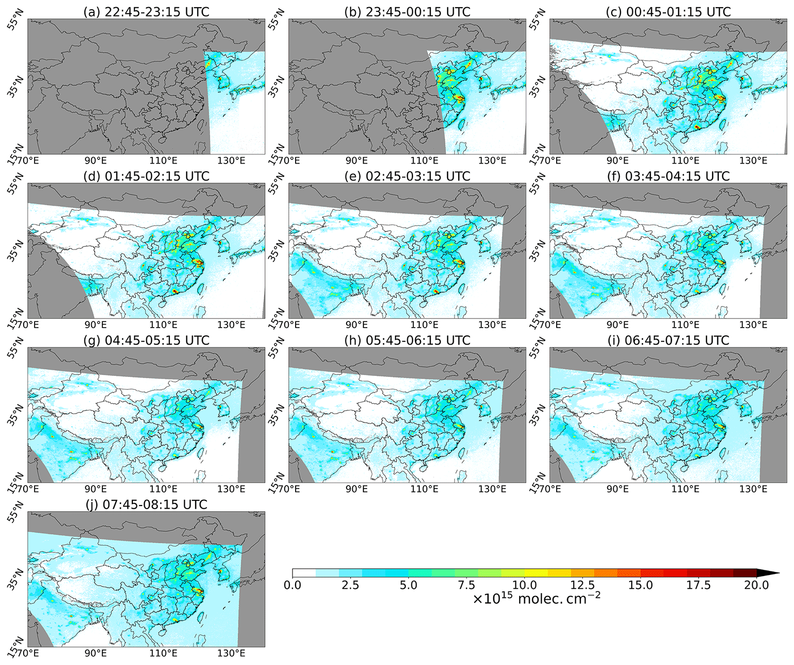
Figure 4Spatial distribution of POMINO–GEMS tropospheric NO2 VCDs at each hour on a 0.05∘ × 0.05∘ grid in JJA 2021. The regions in gray mean that there are no valid observations.
Figure 5a–c present NO2 VCDs in the morning, noon and afternoon in JJA 2021 for eastern China. Data are averaged at 22:45–01:45 UTC (06:45–09:45 Beijing Time, BJT), 02:45–04:45 UTC (10:45–12:45 BJT) and 05:45–07:45 UTC (13:45–15:45 BJT) to represent the morning, noon and afternoon, respectively. In the morning (Fig. 5a), there are clear city signals with high-NO2 values, reflecting abundant NOx emissions from traffic. The spatial gradients of NO2 from urban centers to outskirts are very strong. However, these spatial gradients are greatly reduced in the noon and afternoon (Fig. 5b and c). For example, the differences in the tropospheric NO2 VCDs between the urban center of Xi'an (108.93∘ N, 34.27∘ E) and its surrounding areas (within 50 km) are reduced from about 8×10¹⁵ in the morning to about 4×10¹⁵ at noon and then to below 2×10¹⁵ in the afternoon. This is likely due to chemical loss of traffic-associated NO2, increased emissions from other sectors (e.g., industry) and/or enhanced horizontal transport smearing the spatial gradient.
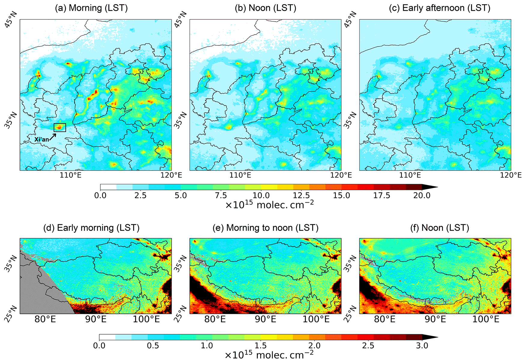
Figure 5Spatial distribution of 3 h mean POMINO–GEMS tropospheric NO2 VCDs in JJA 2021 on a 0.05∘ × 0.05∘ grid. The first row is for eastern China in the (a) morning (22:45–01:45 UTC), (b) noon (02:45–04:45 UTC) and (c) afternoon (05:45–07:45 UTC). The second row is for western China in the (d) early morning (00:45–01:45 UTC), (e) morning to noon (02:45–04:45 UTC) and (f) noon (05:45–07:45 UTC). The regions in gray mean that there are no valid observations.
Over western China with low tropospheric NO2 VCDs (Fig. 5d–f), there is a gradual increase in the tropospheric NO2 by about 1 × 10¹⁵ from the early morning to noon. This increase is likely dominated by biogenic NOx emissions that are sensitive to sunshine intensity and surface temperature (Kong et al., 2023; Weng et al., 2020). Future studies are needed to understand the exact causes.
Figure 6 shows the diurnal variation in the POMINO–GEMS tropospheric NO2 VCDs over six different region groups in the GEMS FOV. The six groups are defined based on the levels of mean POMINO–GEMS tropospheric NO2 VCDs at 12:00 LST in JJA 2021 (VCD12:00 LST), and their spatial distributions are also shown in each panel. We convert the observation time from UTC to LST for each time zone in this domain (+5 time zone at 70–82.5∘ E; +6 time zone at 82.5–97.5∘ E; +7 time zone at 97.5–112.5∘ E; +8 time zone at 112.5–127.5∘ E; +9 time zone at 127.5–140∘ E) and show the NO2 diurnal variations in each time zone with different colors. For low-NO2 situations ( ), NO2 grow in the morning in the +5 and +6 time zones but not in other time zones. Over high-NO2 situations ( ; in cities and suburban areas), NO2 in all time zones exhibits a minimum around noontime and a morning peak at 09:00–10:00 LST, which is consistent with previous findings for specific polluted locations (Boersma et al., 2008, 2009; J. Li et al., 2021; Ghude et al., 2020; Herman et al., 2019; Biswas and Mahajan, 2021). In all groups and time zones, tropospheric NO2 VCDs grow from noon to the afternoon.
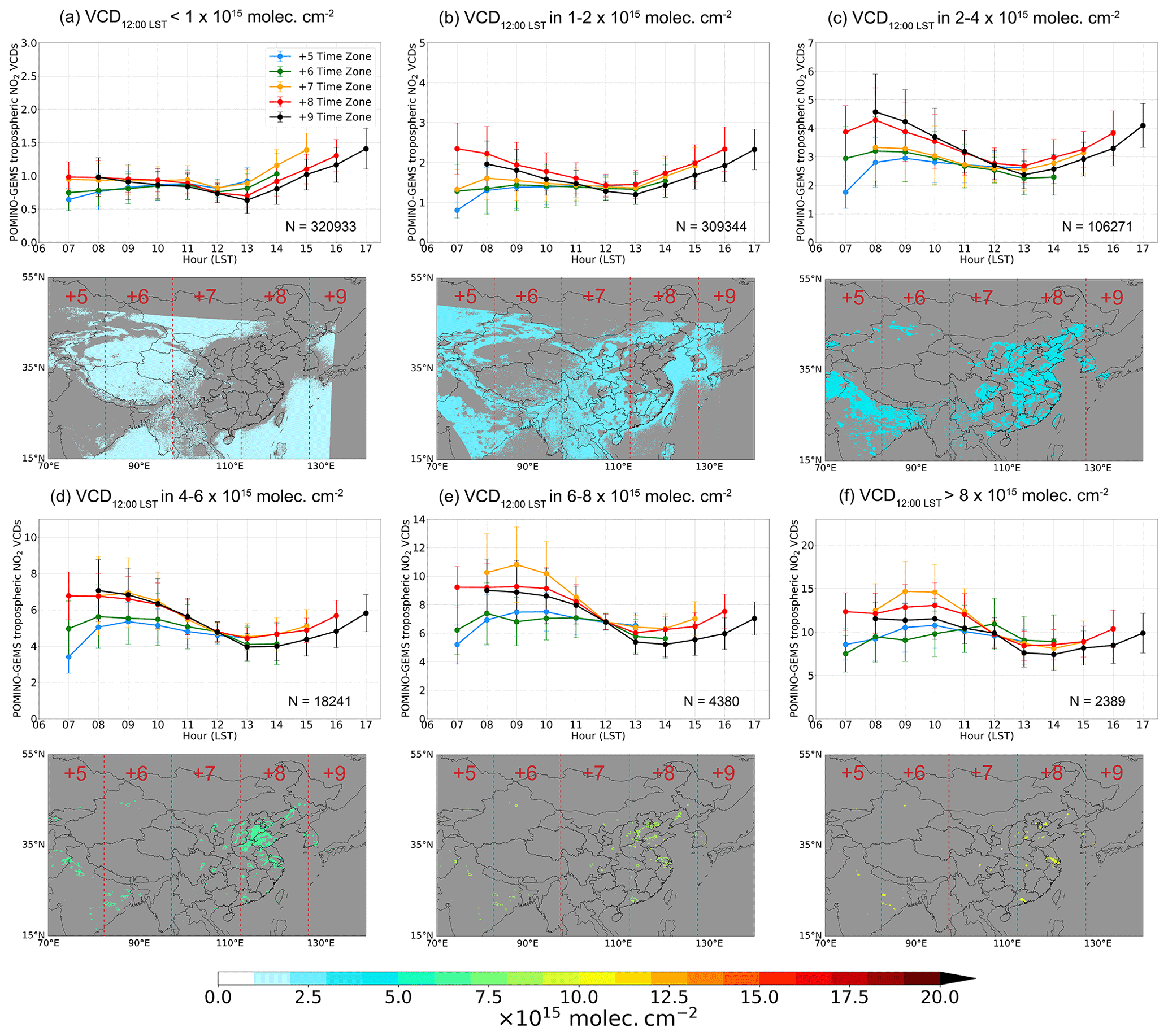
Figure 6POMINO–GEMS NO2 diurnal variations for six region groups classified based on mean POMINO–GEMS tropospheric NO2 VCDs at 12:00 LST in JJA 2021 (VCD12:00 LST). (a) VCD12:00 LST is less than 1 × 10¹⁵ . (b) VCD12:00 LST is 1–2 × 10¹⁵ . (c) VCD12:00 LST is 2–4 × 10¹⁵ . (d) VCD12:00 LST is 4–6 × 10¹⁵ . (e) VCD12:00 LST is 6–8 × 10¹⁵ . (f) VCD12:00 LST is larger than 8 × 10¹⁵ . In each panel, different colors denote the NO2 diurnal variation in different time zones. N denotes the total number of valid 0.05∘ × 0.05∘ grid cells in each region. The error bars denote the standard deviation of tropospheric NO2 VCDs at each hour in each time zone.
The NO2 diurnal variations are related to multiple driving factors. Different sources with distinctive diurnal patterns dominate the NOx emissions over different regions. Lightning and biogenic activities are the major emission sources over low-NO2 land areas, and they tend to intensify with temperature and radiation in the daytime. Anthropogenic emissions are dominant over polluted cities and suburban areas, where the traffic emissions tend to peak in the mid-morning and late afternoon (Jing et al., 2016; Y.-H. Liu et al., 2018; Naiudomthum et al., 2022). In addition, the photochemistry plays an important role. NO2 is in chemical balance with NO, and the ratio of NO2 and NO depends on radiation, ozone and peroxyl radicals. NOx is oxidized to nitric acid and organic nitrates by radicals in the daytime, the level of which depends on radiation, ozone and volatile organic compounds. Thus, the lifetime of NO2 reaches the minimum value around noon, i.e., a few hours in summer. Furthermore, atmospheric transport also affects the diurnal variation in the NO2 at high-value places (e.g., cities) and their surroundings. Further studies are needed to determine the exact causes of NO2 diurnal variations at individual places.
3.2 Comparison with POMINO–TROPOMI v1.2.2, OMNO2 v4 and GOME-2 GDP 4.8 NO2 VCD products
Figure 7a and b show the POMINO–GEMS and POMINO–TROPOMI v1.2.2 tropospheric NO2 VCDs, respectively, on a 0.05∘ × 0.05∘ grid averaged over JJA 2021. Cloud screening is implemented based on the CRFs from each product. To ensure temporal compatibility, matching between hourly GEMS observations and the TROPOMI data at the closest observation time is done for each day. Overall, POMINO–GEMS agrees well with POMINO–TROPOMI with a spatial correlation coefficient of 0.98, a linear regression slope of 1.18 and a small positive NMB of 4.9 % (Fig. 7c). Regionally, POMINO–GEMS VCDs are higher than those of POMINO–TROPOMI v1.2.2 over eastern China, most of India and the northwestern GEMS FOV but smaller over western China and the oceans (Fig. 7a and b; see Fig. S9c and d for plots showing the differences). These differences are related to tropospheric NO2 AMFs and SCDs. A detailed discussion is given in Sect. S3.
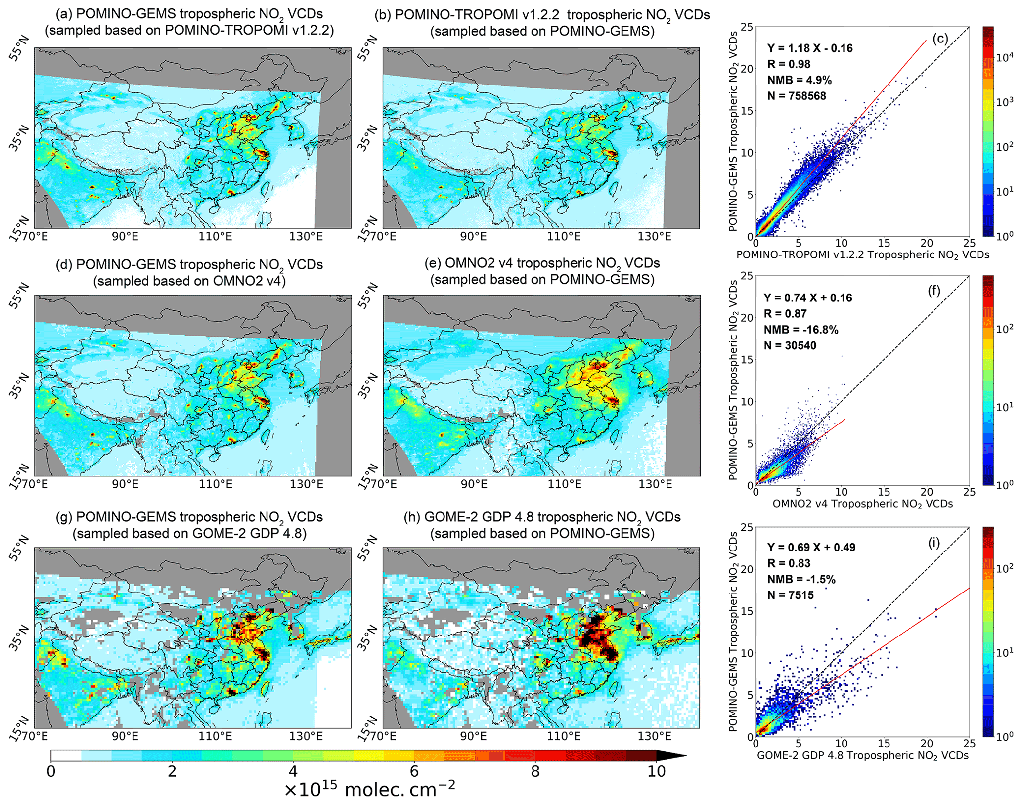
Figure 7Comparison between POMINO–GEMS and other products for tropospheric NO2 VCDs in JJA 2021. (a, b) Between POMINO–GEMS and POMINO–TROPOMI v1.2.2 on a 0.05∘ × 0.05∘ grid, (d, e) between POMINO–GEMS and OMNO2 v4 on a 0.25∘ × 0.25∘ grid and (g, h) between POMINO–GEMS and GOME-2 GDP 4.8 on a 0.5∘ × 0.5∘ grid. Panels (c), (f) and (i) are the respective scatterplots in which the colors represent the data density. The regions in gray mean there are no valid observations.
Figure 7d–f and g–i show the comparison results of POMINO–GEMS tropospheric NO2 VCDs with OMNO2 v4 on a 0.25∘ × 0.25∘ grid and GOME-2 GDP 4.8 on a 0.5∘ × 0.5∘ grid averaged over JJA 2021, respectively. POMINO–GEMS NO2 VCDs exhibit good spatial consistency with the two independent products (R=0.87 and 0.83), although with slightly lower values than OMNO2 v4 (by 16.8 %) and GOME-2 GDP 4.8 (by 1.5 %). These VCD differences are expected, considering the differences in the retrieval algorithm. For example, the POMINO–GEMS algorithm implements explicit aerosol corrections in the radiative transfer calculation, while OMNO2 v4 and GOME-2 GDP 4.8 treat aerosols as “effective clouds”. POMINO–GEMS accounts for the anisotropy of surface reflectance by adopting MODIS BRDF coefficients, whereas OMNO2 v4 and GOME-2 GDP 4.8 use geometry-dependent and regular LER, respectively. The horizontal resolution of a priori NO2 profiles in POMINO–GEMS is 25 km (and interpolated to 2.5 km), 1∘ × 1.25∘ in OMNO2 v4 and 1.875∘ × 1.875∘ in GOME-2 GDP 4.8 (Valks et al., 2019a; Lamsal et al., 2021).
Based on comparisons with POMINO–TROPOMI v1.2.2, OMNO2 v4 and GOME-2 GDP 4.8 NO2 VCDs, we conclude that POMINO–GEMS NO2 columns show good agreement with LEO satellite data, with values lower by 20 % at most.
3.3 Validation with MAX-DOAS NO2 VCD measurements
The scatterplot in Fig. 8a compares POMINO–GEMS tropospheric NO2 VCDs in JJA 2021 at all GEMS observation hours with matched ground-based MAX-DOAS measurements at nine sites. POMINO–GEMS correlates with MAX-DOAS (R=0.66), with a small negative bias (NMB = −11.1 %). The linear regression shows a slope of 0.51 and intercept of 3.34×10¹⁵ , reflecting underestimation of POMINO–GEMS tropospheric NO2 VCDs on high-NO2 days.
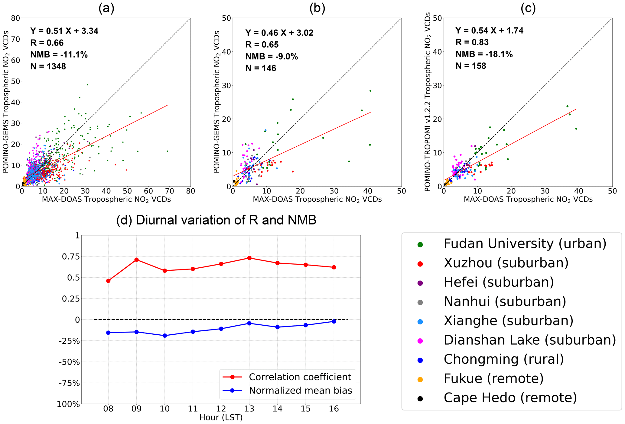
Figure 8Evaluation of satellite NO2 VCD data using ground-based MAX-DOAS measurements. (a) Scatterplot for tropospheric NO2 VCDs (× 1015 ) between MAX-DOAS and POMINO–GEMS at all GEMS observation hours in JJA 2021. Each data pair denotes an hour. (b, c) Scatterplots for tropospheric NO2 VCDs (×1015 ) in JJA 2021 (b) between MAX-DOAS and POMINO–GEMS at 13:45–14:15 LST and (c) between MAX-DOAS and POMINO–TROPOMI v1.2.2. Each data pair denotes a day. Each MAX-DOAS station is color-coded. (d) Diurnal variations in the spatiotemporal correlation coefficients and NMBs of POMINO–GEMS tropospheric NO2 VCDs relative to ground-based MAX-DOAS data.
Figure 8b and c further use MAX-DOAS measurements to evaluate POMINO–GEMS and POMINO–TROPOMI v1.2.2 tropospheric NO2 VCDs at the overpass time of TROPOMI. In Fig. 8b, POMINO–GEMS data at 13:45–14:15 LST are used to match the overpass time of TROPOMI. The POMINO–TROPOMI product is evaluated in the context of understanding the relative performance of POMINO–GEMS. Each data point represents a day. Figure 8b and c show that the day-to-day variability in the MAX-DOAS measurements is well captured by POMINO–TROPOMI v1.2.2 (R=0.83) but less so by POMINO–GEMS (R=0.65). Linear regression results show an underestimate of tropospheric NO2 VCDs in POMINO–TROPOMI v1.2.2 (NMB = −18.1 %), as also found in previous studies (Liu et al., 2020). POMINO–GEMS exhibits a small bias (NMB = −9.0 %), but the station-dependent performance is apparent. At the two remote sites of Fukue and Cape Hedo with low NO2, POMINO–GEMS NO2 columns are higher than those of MAX-DOAS measurements. At the other sites, the data pairs are more scattered and located both above and below the 1:1 line, resulting in a small NMB.
Figure 8d shows the NMBs and correlation coefficients of POMINO–GEMS NO2 VCDs relative to ground-based MAX-DOAS data at each hour. The negative NMBs reach a maximum of about 20 % at 10:00 LST and decrease to less than 10 % in the afternoon. The correlation coefficients are modest or high (0.45–0.73) at all hours.
Figure 9 compares the diurnal variation in the tropospheric NO2 VCDs between POMINO–GEMS and MAX-DOAS at eight stations. At each site, NO2 values are averaged in JJA 2021 at each hour for comparison, and the number of valid days for each hour is also shown. The Cape Hedo site is not included because there are few valid MAX-DOAS data points at each hour. Figure 9a–f show that at the urban and suburban sites, MAX-DOAS NO2 (black lines) peaks in the mid-to-late morning, declines towards the minimum values at noon around 13:00 LST and then gradually increases in the afternoon. A strong correlation of NO2 diurnal variation between POMINO–GEMS (solid red lines) and MAX-DOAS is found at Xuzhou (R=0.82), Hefei (R=0.96), Fudan University (R=0.84), Nanhui (R=0.79) and Xianghe (R=0.94). At the Dianshan Lake site, POMINO–GEMS NO2 columns increase, but MAX-DOAS data decrease from 08:00 to 09:00 LST, resulting in a lower correlation coefficient (R=0.60). At Chongming and Fukue sites, MAX-DOAS NO2 shows a peak in the morning without an evident increase in the early afternoon, but this diurnal pattern is not fully captured by POMINO–GEMS. At Fukue, POMINO–GEMS NO2 exhibits abrupt changes at 12:00 and 13:00 LST due to few valid data points.
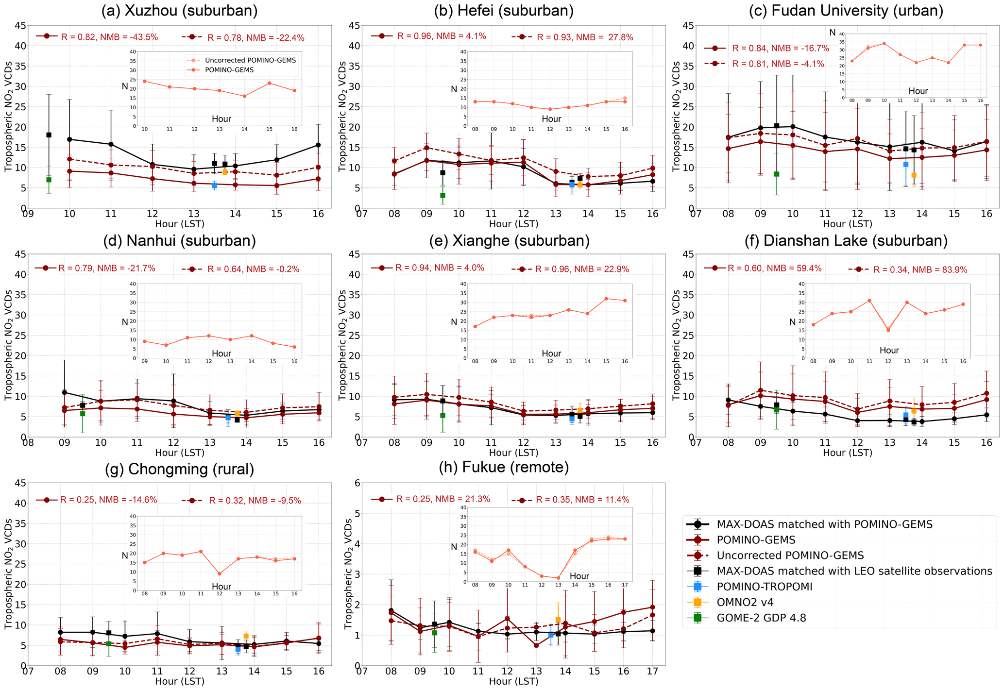
Figure 9Diurnal variation in the hourly tropospheric NO2 VCDs (× 1015 ) of MAX-DOAS (black lines), POMINO–GEMS with TROPOMI correction (solid red lines) and re-calculated POMINO–GEMS without TROPOMI correction (dashed red lines) at eight sites in JJA 2021. The error bars denote the standard deviation of MAX-DOAS and POMINO–GEMS NO2 at each hour, respectively. The diurnal correlation and all-hour mean NMB of POMINO–GEMS against MAX-DOAS data are shown. The number of valid days for each hour is also presented. The black squares with an error bar represent the mean value and standard deviation of MAX-DOAS tropospheric NO2 VCDs matched with POMINO–TROPOMI v1.2.2 (blue squares), OMNO2 v4 (orange squares) and GOME-2 GDP 4.8 (green squares), respectively.
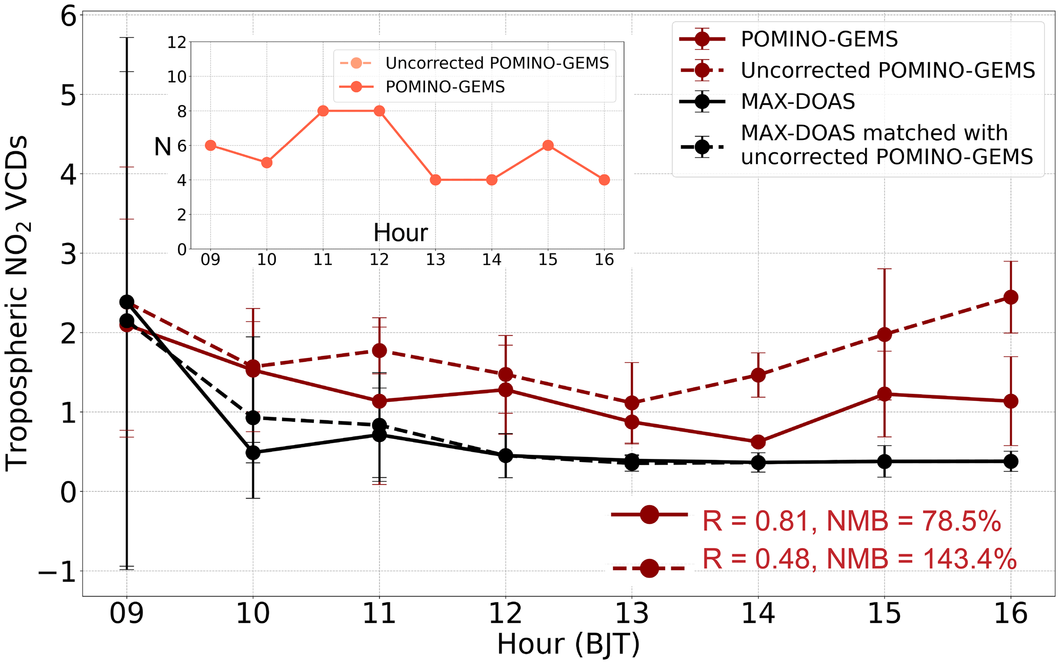
Figure 10Diurnal variation in the hourly mean tropospheric NO2 VCDs (× 1015 ) of mobile car MAX-DOAS and POMINO–GEMS in the Three Rivers source region. The solid black lines denote MAX-DOAS data that spatiotemporally match with POMINO–GEMS with total SCD correction (solid red lines). The dashed black lines denote MAX-DOAS data that spatiotemporally match with POMINO–GEMS without correction (dashed red lines). The error bars denote the standard deviation of MAX-DOAS and POMINO–GEMS NO2 at each hour during the field campaign, respectively. Values for diurnal correlation and mean NMB of POMINO–GEMS relative to MAX-DOAS are shown. The number of days with valid data for each hour is also presented.
In addition, comparison of POMINO–GEMS diurnal variation with NO2 data from GOME-2 in the morning and OMI and TROPOMI in the early afternoon shows good agreement at Hefei, Nanhui, Dianshan Lake, Chongming and Fukue sites. The differences between POMINO–GEMS and MAX-DOAS NO2 VCDs are comparable to or smaller than those between LEO satellite and MAX-DOAS NO2 VCDs.
As we use TROPOMI total NO2 SCDs to correct those of GEMS, this may influence the NO2 diurnal variation in the original GEMS observations. Thus we also compare MAX-DOAS data with re-calculated POMINO–GEMS tropospheric NO2 VCDs without correction in total SCDs (dashed red lines in Fig. 9). Compared to our default POMINO–GEMS data (with correction), excluding the correction leads to lower diurnal correlation coefficients at Xuzhou, Hefei, Fudan University, Nanhui and Dianshan Lake but higher correlation coefficients at Xianghe, Chongming and Fukue. Excluding the correction increases the NMB at three sites but decreases the NMB at five sites. We conclude that at these eight sites (in the eastern areas), no significant influence on the diurnal variation in the POMINO–GEMS tropospheric NO2 VCDs is brought in through TROPOMI-based correction for total NO2 SCDs.
Figure 10 compares the diurnal variations between POMINO–GEMS and mobile car MAX-DOAS tropospheric NO2 VCD data in the Three Rivers source region on the Tibetan Plateau. Results of POMINO–GEMS with and without total SCD correction are shown in the solid and dashed red lines, respectively. Mobile car MAX-DOAS data show an evident decrease in the tropospheric NO2 VCDs from the morning to noon, with little change thereafter. Such NO2 diurnal patterns reflect the spatial and temporal variations in the tropospheric NO2 along the driving route. The high-NO2 values with large standard deviation at 09:00 BJT are due to enhanced pollution and variability in the morning when the mobile car is in or near Xining city. The NO2 diurnal variations in the POMINO–GEMS with correction correlate well with those of mobile car MAX-DOAS data (R=0.81). In contrast, POMINO–GEMS without total SCD correction exhibits much poorer correlation with mobile car MAX-DOAS data, due to the erroneous increase in the afternoon.
Overall, the validation results with independent ground-based and mobile car MAX-DOAS measurements provide confidence on the general characteristics of POMINO–GEMS NO2 diurnal variations.
3.4 Validation with surface NO2 concentration measurements from MEE
The scatterplot in Fig. 11a compares surface NO2 concentrations derived from POMINO–GEMS with MEE measurements at all hours. POMINO–GEMS-derived surface NO2 concentrations show good agreement with MEE measurements in terms of spatiotemporal correlation (R=0.78) and bias (NMB = −26.3 %) but are higher than those of MEE at some high-value situations, which mainly occur over the YRD region (Fig. S14). These differences reflect errors in POMINO–GEMS NO2 VCDs themselves, errors in the conversion process from tropospheric NO2 VCDs to surface concentrations, and errors in the MEE data (due to potential contamination by nitric acid and organic nitrates; M. Liu et al., 2018).
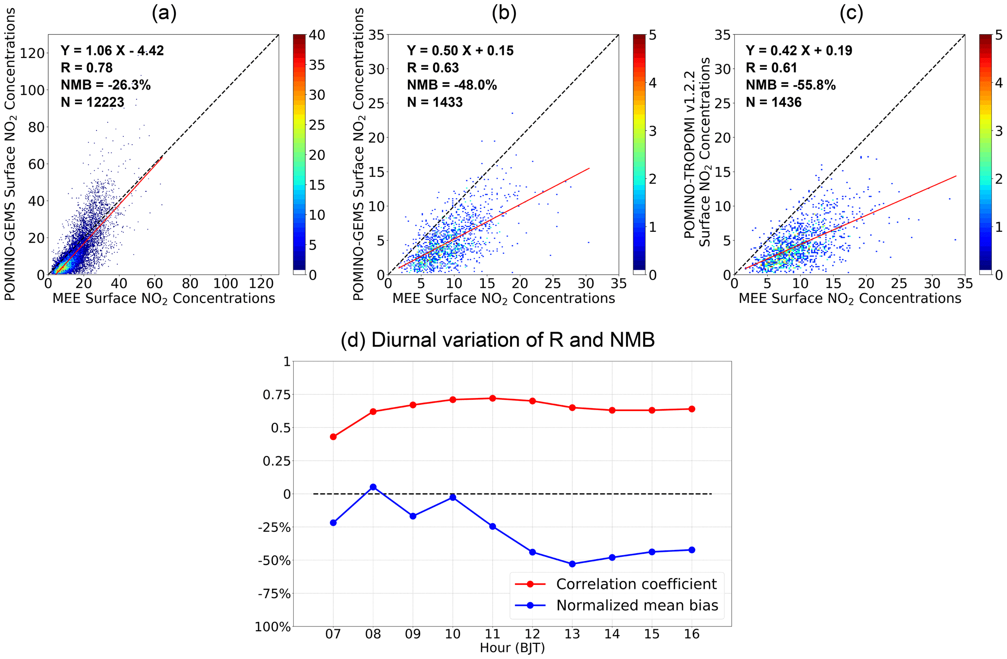
Figure 11Evaluation of satellite-derived surface NO2 concentrations (µg m−3) using MEE measurements in JJA 2021. (a) Scatterplot for MEE and POMINO–GEMS at all GEMS observation hours averaged over all days in JJA 2021. (b) Scatterplot for MEE and POMINO–GEMS at 13:45–14:15 LST. (c) Scatterplot for MEE and POMINO–TROPOMI v1.2.2. The color bar represents the data density. (d) Diurnal variations in the spatiotemporal correlation coefficients and NMBs of POMINO–GEMS-derived surface NO2 concentrations relative to MEE measurements.
Figure 11b and c show the validation results for satellite-derived surface NO2 concentrations with MEE measurements at the overpass time of TROPOMI (i.e., early afternoon). Here, each data pair denotes a MEE site. POMINO–GEMS results at 13:45–14:15 LST are used to match the overpass time of TROPOMI data. Overall, both satellite-based datasets show good spatial correlation with MEE measurements (R=0.63 and 0.61). POMINO–GEMS exhibits higher linear regression slope (0.50) with a smaller NMB (−48.0 %). The values of satellite data are lower than those from MEE, especially in the afternoon (Fig. 11d). This is in part because of the aforementioned contamination issues in MEE data, which becomes more severe in the afternoon as the air ages throughout the daytime.
Figure 12a examines the diurnal variation in the surface NO2 concentrations averaged over JJA 2021 at all sites. The MEE data show a smooth and monotonic decline from the early morning to the early afternoon, with a slight increase beginning at 15:00 LST. This diurnal pattern differs from those seen in ground-based MAX-DOAS VCD data (Fig. 9), due to the difference in sampling size between MEE and MAX-DOAS, the diurnal variation in the NO2 vertical distribution that affects the relationship between surface and columnar NO2 and the insensitivity of NO2 columns to changes in PBL heights. POMINO–GEMS-derived surface NO2 concentrations show similar diurnal variations to those of MEE (R=0.97), although with a peak at 10:00 LST and a gradual increase beginning at 14:00 LST. The discrepancies between POMINO–GEMS and MEE surface NO2 concentrations at different hours are likely caused by the assumed constant correction factor of 2 to account for the vertical gradient of NO2 from the height of the ground instrument to the center of the first model layer (Sect. 2.2). In the morning when the PBL is low, most NO2 molecules are near the ground, and the vertical gradient of NO2 over polluted regions is the largest in the daytime, so the factor of 2 may lead to the underestimation of derived surface NO2 concentrations. In contrast, in the afternoon, the PBL mixing is much stronger, and the vertical gradient of NO2 is much smaller; thus, the factor of 2 may lead to overestimated surface NO2 concentrations. Note that the consistency between POMINO–GEMS and MEE data does not depend on the total SCD correction (Table S4).
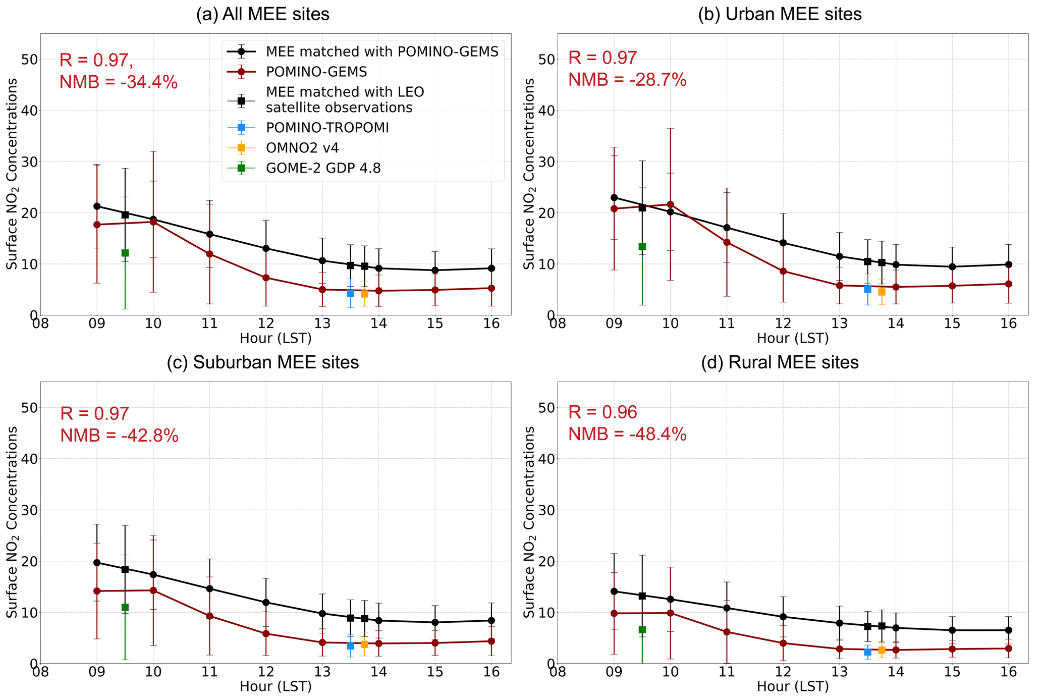
Figure 12Diurnal variation in the hourly surface NO2 concentrations (µg m−3) of MEE (back lines) and POMINO–GEMS (red lines) in JJA 2021 (a) at all MEE sites, (b) at urban sites, (c) at suburban sites and (d) at rural sites. The error bars denote the standard deviation of MEE and POMINO–GEMS-derived surface NO2 concentrations at each hour in JJA 2021, respectively. Diurnal correlation and mean NMB of POMINO–GEMS relative to MEE are also listed. The black squares with an error bar represent the mean value and standard deviation of MEE data matched with POMINO–TROPOMI v1.2.2 (blue squares), OMNO2 v4 (orange squares) and GOME-2 GDP 4.8 (green squares), respectively.
To quantify the influences of the diurnal variation in the hourly column-to-surface ratio from GEOS-Chem simulations, we compare the MEE measurements with POMINO–GEMS-derived surface NO2 concentrations using daily column-to-surface ratio (Fig. S15). As expected, POMINO–GEMS-derived NO2 concentrations show a similar diurnal variation to the tropospheric NO2 VCDs, with two peaks in the mid-morning and afternoon and a minimum at noon. The temporal correlation coefficient with MEE is only about 0.23. Thus, it is more reasonable to use an hourly ratio for comparison with MEE measurements, as done in our study.
To further test the reliability of our VCD-to-surface-concentration conversion method (Eq. 9), we apply the same method to MAX-DOAS NO2 VCDs and compare the resulting surface NO2 concentrations with MEE data. As shown in Fig. S16, the diurnal variation in the MAX-DOAS-derived surface NO2 concentrations correlates well with that of MEE measurements (R=0.96), which supports our conversion method.
Figure 12b–d show the comparison of NO2 diurnal variations for different groups of MEE sites. The diurnal variations in the POMINO–GEMS-derived surface NO2 concentrations show similar characteristics over urban, suburban and rural regions, and all results correlate well with those of MEE data. Meanwhile, surface NO2 concentrations derived from LEO satellite observations also agree well with those of POMINO–GEMS, except GOME-2-GDP-4.8-derived surface NO2 concentrations, which are lower than those of POMINO–GEMS by about 30 %–40 %. We conclude that the validation with extensive MEE measurements presents a promising performance of the POMINO–GEMS retrievals, especially the great agreement of the POMINO–GEMS NO2 diurnal variation with MEE data over urban, suburban and rural regions.
3.5 Error estimates for POMINO–GEMS tropospheric NO2 VCDs
Total retrieval errors for POMINO–GEMS tropospheric NO2 VCDs are derived from the calculations of total SCDs, stratospheric SCDs and tropospheric AMFs. Spatial and temporal averaging across GEMS pixels greatly reduces the random errors but hardly affects the systematic errors. Here, we provide a preliminary estimate of POMINO–GEMS errors for the summertime retrieval discussed above.
As described in Sect. 2, we calculate hourly total SCDs based on the original GEMS SCD data and daily TROPOMI-guided corrections. According to the GEMS ATBD of the NO2 retrieval algorithm, the SCD errors from the DOAS method are < 5.65 % at high-NO2 conditions (NO2 VCD ; Park et al., 2020). The NO2 SCD errors in TROPOMI are reported to be 0.5–0.6 ×10¹⁵ (10 % in a relative sense; Van Geffen et al., 2022a). Given the assumption we made in adjusting GEMS total SCDs to match TROPOMI values, we tentatively estimate the error in our corrected total SCD data to be 0.5–0.7 ×10¹⁵ (10 % in a relative sense) for most regions and 0.9×10¹⁵ (20 %–30 %) at the edge of the northwestern GEMS FOV.
In constructing the stratospheric NO2 SCDs, the stratospheric VCDs are taken from TROPOMI PAL v2.3.1, scaled based on GEOS-CF v1 stratospheric NO2 to account for diurnal variation and then applied with geometric AMFs. We assign a constant error of 0.2×10¹⁵ (5 %–10 %) to our hourly stratospheric SCDs, which is the same as the value for TROPOMI (Van Geffen et al., 2022a). Few studies have assessed the accuracy of stratospheric NO2 and its diurnal variation from GEOS-CF data (Knowland et al., 2022), but our comparison between GEOS-CF and TROPOMI shows great consistency (Sect. 2.1.5). As most of the errors in total SCDs are absorbed in the stratosphere–troposphere separation step (Van Geffen et al., 2015), the errors in tropospheric SCDs should be 10 %–30 %, depending on different cases, with higher relative biases in cleaner situations.
Tropospheric AMF calculations are the dominant error source for the retrieved tropospheric NO2 VCDs over polluted regions. According to Liu et al. (2020), the AMF errors caused by uncertainty in surface reflectance are about 10 %, and errors induced by uncertainties in aerosol parameters are about 10 % in clean regions and 20 % for heavily polluted situations. We further assume that the O2–O2 cloud retrieval algorithm introduces another error at the 10 % level to the NO2 AMFs. The uncertainty in a priori NO2 vertical profiles is estimated to cause an AMF error of 10 % (Liu et al., 2020). Yang et al. (2023) suggested that the NO2 profiles from GEOS-Chem (version 13.3.4) might contain incorrect timing of PBL mixing growth in the morning and thus introduce a relative root mean square error of 7.6 % and NMB of 2.7 % in AMF; however, this error could be greatly dampened by averaging over a long time period. The free tropospheric NO2 bias in GEOS-Chem NO2 profiles might also contribute to the retrieval errors, especially over remote regions. Adding these errors in quadrature leads to the overall AMF errors for POMINO–GEMS at 20 %–40 %.
The overall uncertainty in POMINO–GEMS tropospheric NO2 VCDs is estimated by adding in quadrature the errors in tropospheric NO2 SCDs and AMFs, which is when these errors are expressed in the relative sense. For remote regions with low tropospheric NO2 abundances, the overall retrieval uncertainties can reach 30 %–50 % and are dominated by errors in tropospheric SCDs. For regions with abundant tropospheric NO2, the uncertainties in the retrieved tropospheric VCDs are dominated by the AMF errors and are estimated to be about 20 %–30 %.
As shown in Figs. 8d and 11d, the maximum negative NMB of POMINO–GEMS tropospheric NO2 VCDs relative to ground-based MAX-DOAS data is about 20 % in the mid-morning, and the NMB of POMINO–GEMS-derived surface NO2 concentrations to MEE measurements is −30 % on average. Thus, our estimated error magnitude is supported by the independent ground-based MAX-DOAS and MEE data.
The GEMS instrument provides an unprecedented opportunity for air quality monitoring at a high spatiotemporal resolution. Our POMINO–GEMS algorithm retrieves tropospheric NO2 VCDs as a research product. The algorithm first calculates hourly tropospheric NO2 SCDs through the fusion of total NO2 SCDs from the GEMS v1.0 L2 NO2 product, total and stratospheric NO2 columns from the TROPOMI PAL v2.3.1 L2 NO2 product and stratospheric NO2 diurnal variations from the GEOS-CF v1 dataset. The fusion approach reduces the high bias in total SCDs and removes the stripe-like patterns in the official GEMS v1.0 product. Our algorithm then calculates tropospheric NO2 AMFs to convert SCDs to VCDs. A preliminary estimate of retrieval errors is also given.
Our initial POMINO–GEMS data for JJA 2021 show high values of tropospheric NO2 VCDs, with clear hotspots ( ) over regions where anthropogenic emissions of NOx are abundant. The spatial gradients of tropospheric NO2 VCDs from urban centers to surrounding areas are substantial in the morning due to traffic emissions, but the gradients are much reduced at noon and in the afternoon. A gradual increase in the tropospheric NO2 VCDs from the morning to noon is observed over clean regions of western China, likely as a result of enhanced biogenic emissions. Over high-NO2 regions, where anthropogenic activities dominate the NOx emissions, NO2 columns increase until a peak at 09:00–10:00 LST, decrease to the minimum at noon and then increase in the afternoon again. Such characteristics of NO2 diurnal variations are associated with the changes in natural and anthropogenic NOx emissions, photochemistry and atmospheric transport.
POMINO–GEMS tropospheric NO2 VCDs agree well with POMINO–TROPOMI v1.2.2 in terms of spatial correlation (0.98) and NMB (4.9 %). POMINO–GEMS data are also consistent with the OMNO2 v4 tropospheric NO2 VCD product in the early afternoon and GOME-2 GDP 4.8 tropospheric NO2 VCD product in the morning, with R of 0.87 and 0.83 and NMB of −16.8 % and −1.5 %, respectively.
POMINO–GEMS tropospheric NO2 VCDs are comparable with ground-based MAX-DOAS measurements at nine ground-based sites with a small NMB (−11.1 %), although the correlation is modest (R=0.66). Both the bias and correlation values are smaller than POMINO–TROPOMI v1.2.2 (NMB = −18.1 %; R=0.83). More importantly, POMINO–GEMS well captures the diurnal variation in the MAX-DOAS NO2 VCDs at Xuzhou (R=0.82), Hefei (R=0.96), Fudan University (R=0.84), Nanhui (R=0.79), Xianghe (R=0.94) and Dianshan Lake (R=0.60) sites, although the correlations are relatively poor at Chongming and Fukue sites. Comparison with mobile car MAX-DOAS measurements in the Three Rivers source region on the Tibetan Plateau also shows good correlation in NO2 diurnal variation (R=0.81).
We also compare surface NO2 concentrations derived from tropospheric NO2 VCDs in POMINO–GEMS and POMINO–TROPOMI v1.2.2 against MEE data, taking advantage of the large number of MEE sites. POMINO–GEMS-derived surface NO2 concentration data exhibit a small NMB (−26.3 %). For these sites at TROPOMI overpass times, POMINO–GEMS-derived surface NO2 concentrations show a smaller magnitude of NMB (−48.0 %) than POMINO–TROPOMI v1.2.2 (−55.8 %). Excellent agreement in the diurnal variation between POMINO–GEMS-derived and MEE NO2 is exhibited over all (R=0.97), urban (R=0.97), suburban (R=0.97) and rural (R=0.96) sites.
Overall, our comprehensive validation process highlights the good performance of POMINO–GEMS tropospheric NO2 VCD product, both in magnitude and spatiotemporal variation. However, there are still several limitations in our study. To address the systematic overestimation and stripes problems in the original GEMS data, we correct GEMS total NO2 SCDs by using TROPOMI data as a temporary solution. For example, we implement a simple geometric correction to combine GEMS and TROPOMI total NO2 SCDs, but their differences in scattering geometry are only partly accounted for. Thus this correction works well in most regions but may introduce SCD uncertainties up to 0.9×10¹⁵ (20 %–30 %) at the edge of the northwestern GEMS FOV. Currently, the Environmental Satellite Center of South Korea is updating the NO2 SCD data to v2.0. We will update our POMINO–GEMS algorithm accordingly, once the updated official NO2 product becomes available, to provide necessary inputs for our research product. In addition, in the conversion from NO2 VCDs to surface concentrations, we use a constant correction factor of 2 to account for the strong NO2 vertical gradient near the surface. This simple treatment does not account for the diurnal variation in the correction factor and thus may introduce errors in the derived surface NO2 concentrations. Nevertheless, the current POMINO–GEMS data serve as our initial attempt to derive the diurnal variations in the tropospheric NO2 at a high spatiotemporal resolution from GEMS, and they are expected to offer a useful source of information for various applications such as air quality analysis and emission constraint.
The POMINO-GEMS NO2 data are freely available on the ACM group product website (http://www.pku-atmos-acm.org/acmProduct.php/, Lin et al., 2023). The GEMS v1.0 NO2 product used here can be downloaded from https://nesc.nier.go.kr/ko/html/index.do (National Institute of Environmental Research, NIER, 2023). The reprocessed TROPOMI PAL v2.3.1 L2 product can be downloaded from https://data-portal.s5p-pal.com/products/no2.html (S5P PAL Data Portal, 2022). The OMNO2 v4 L2 product can be downloaded from https://doi.org/10.5067/Aura/OMI/DATA2017 (Krotkov et al., 2019). The GOME-2 GDP 4.8 L2 product can be downloaded from http://acsaf.org/ (EUMETSAT, 2023) after registration. The GEOS-CF v1.0 dataset can be downloaded from https://portal.nccs.nasa.gov/datashare/gmao/geos-cf/ (NASA, 2023). The MEE surface NO2 measurements can be downloaded from http://www.cnemc.cn/sssj/cskqzl/ (Ministry of Ecology and Environment, 2023). The ground-based and mobile car MAX-DOAS measurements can be provided upon request to the corresponding authors.
The supplement related to this article is available online at: https://doi.org/10.5194/amt-16-4643-2023-supplement.
JL conceived this research. YZ and JL designed the algorithm and validation process. YZ performed all calculations, with additional code support from HK. YZ and JL wrote the paper. RS provided LIDORT. JK, HL, JP and HH provided GEMS data. MVR, FH, TiW, PW, QH, KQ, YC, YK, JX, PX, XT, SZ and SW provided the ground-based MAX-DOAS measurements. SC, XC, JM and ThW provided the mobile car MAX-DOAS measurements. HK helped process the MEE measurements. LC and ML helped analyze the validation results. All co-authors commented on the paper.
At least one of the (co-)authors is a member of the editorial board of Atmospheric Measurement Techniques. The peer-review process was guided by an independent editor, and the authors also have no other competing interests to declare.
Publisher's note: Copernicus Publications remains neutral with regard to jurisdictional claims in published maps and institutional affiliations.
This article is part of the special issue “GEMS: first year in operation (AMT/ACP inter-journal SI)”. It is not associated with a conference.
This research has been supported by the National Natural Science Foundation of China (grant no. 42075175) and the Second Tibetan Plateau Scientific Expedition and Research Program (grant no. 2019QZKK0604).
This paper was edited by Helen Worden and reviewed by three anonymous referees.
Beirle, S., Boersma, K. F., Platt, U., Lawrence, M. G., and Wagner, T.: Megacity Emissions and Lifetimes of Nitrogen Oxides Probed from Space, Science, 333, 1737–1739, https://doi.org/10.1126/science.1207824, 2011.
Biswas, M. S. and Mahajan, A. S.: Year-long Concurrent MAX-DOAS Observations of Nitrogen Dioxide and Formaldehyde at Pune: Understanding Diurnal and Seasonal Variation Drivers, Aerosol Air Qual. Res., 21, 200524, https://doi.org/10.4209/aaqr.200524, 2021.
Boersma, K. F., Eskes, H. J., and Brinksma, E. J.: Error analysis for tropospheric NO2 retrieval from space, J. Geophys. Res.-Atmos., 109, D04311, https://doi.org/10.1029/2003jd003962, 2004.
Boersma, K. F., Jacob, D. J., Eskes, H. J., Pinder, R. W., Wang, J., and van der A, R. J.: Intercomparison of SCIAMACHY and OMI tropospheric NO2 columns: Observing the diurnal evolution of chemistry and emissions from space, J. Geophys. Res., 113, D16S26, https://doi.org/10.1029/2007jd008816, 2008.
Boersma, K. F., Jacob, D. J., Trainic, M., Rudich, Y., DeSmedt, I., Dirksen, R., and Eskes, H. J.: Validation of urban NO2 concentrations and their diurnal and seasonal variations observed from the SCIAMACHY and OMI sensors using in situ surface measurements in Israeli cities, Atmos. Chem. Phys., 9, 3867–3879, https://doi.org/10.5194/acp-9-3867-2009, 2009.
Boersma, K. F., Eskes, H. J., Dirksen, R. J., van der A, R. J., Veefkind, J. P., Stammes, P., Huijnen, V., Kleipool, Q. L., Sneep, M., Claas, J., Leitão, J., Richter, A., Zhou, Y., and Brunner, D.: An improved tropospheric NO2 column retrieval algorithm for the Ozone Monitoring Instrument, Atmos. Meas. Tech., 4, 1905–1928, https://doi.org/10.5194/amt-4-1905-2011, 2011.
Burrows, J. P.: The Global Ozone Monitoring Experiment (GOME): Mission concept and first scientific results, J. Atmos. Sci., 56, 2340–2352, 1999.
Callies, J., Corpaccioli, E., Eisinger, M., Hahne, A., and Lefebvre, A.: GOME-2- Metop’s second-generation sensor for operational ozone monitoring, ESA Bull., 102, 28–36, 2000.
Chen, L., Lin, J., Martin, R., Du, M., Weng, H., Kong, H., Ni, R., Meng, J., Zhang, Y., Zhang, L., and van Donkelaar, A.: Inequality in historical transboundary anthropogenic PM2.5 health impacts, Sci. Bull., 67, 437–444, https://doi.org/10.1016/j.scib.2021.11.007, 2021.
Chen, L., Lin, J., Ni, R., Kong, H., Du, M., Yan, Y., Liu, M., Wang, J., Weng, H., Zhao, Y., Li, C., and Martin, R. V.: Historical transboundary ozone health impact linked to affluence, Environ. Res. Lett., 17, 104014, https://doi.org/10.1088/1748-9326/ac9009, 2022.
Cheng, S., Cheng, X., Ma, J., Xu, X., Zhang, W., Lv, J., Bai, G., Chen, B., Ma, S., Ziegler, S., Donner, S., and Wagner, T.: Mobile MAX-DOAS observations of tropospheric NO2 and HCHO during summer over the Three Rivers' Source region in China, Atmos. Chem. Phys., 23, 3655–3677, https://doi.org/10.5194/acp-23-3655-2023, 2023.
Cooper, M. J., Martin, R. V., Hammer, M. S., Levelt, P. F., Veefkind, P., Lamsal, L. N., Krotkov, N. A., Brook, J. R., and Mclinden, C. A.: Global fine-scale changes in ambient NO2 during COVID-19 lockdowns, Nature, 601, 380–387, https://doi.org/10.1038/s41586-021-04229-0, 2022.
Crutzen, P. J.: The influence of nitrogen oxides on the atmospheric ozone content, Q. J. Roy. Meteor. Soc., 96, 320–325, https://doi.org/10.1002/qj.49709640815, 1970.
Cui, Y., Lin, J., Song, C., Liu, M., Yan, Y., Xu, Y., and Huang, B.: Rapid growth in nitrogen dioxide pollution over Western China, 2005–2013, Atmos. Chem. Phys., 16, 6207–6221, https://doi.org/10.5194/acp-16-6207-2016, 2016.
Dirksen, R. J., Boersma, K. F., Eskes, H. J., Ionov, D. V., Bucsela, E. J., Levelt, P. F., and Kelder, H. M.: Evaluation of stratospheric NO2 retrieved from the Ozone Monitoring Instrument: Intercomparison, diurnal cycle, and trending, J. Geophys. Res., 116, D08305, https://doi.org/10.1029/2010jd014943, 2011.
Eastham, S. D., Weisenstein, D. K., and Barrett, S. R. H.: Development and evaluation of the unified tropospheric–stratospheric chemistry extension (UCX) for the global chemistry-transport model GEOS-Chem, Atmos. Environ., 89, 52–63, https://doi.org/10.1016/j.atmosenv.2014.02.001, 2014.
Eskes, H., Van Geffen, J., Sneep, M., Veefkind, P., Niemeier, S., and Zehner, C.: S5P Nitrogen Dioxide v02.03.01 intermediate reproecessing on the S5P-PAL system: Readme file, S5P PAL Data Portal, https://data-portal.s5p-pal.com/products/no2.html (last access: 21 September 2023), 2021.
EUMETSAT: AC SAF (Satellite Application Facility on Atmospheric Composition Monitoring), http://acsaf.org/, last access: 16 April 2023.
Ghude, S. D., Karumuri, R. K., Jena, C., Kulkarni, R., Pfister, G. G., Sajjan, V. S., Pithani, P., Debnath, S., Kumar, R., Upendra, B., Kulkarni, S. H., Lal, D. M., Vander A, R. J., and Mahajan, A. S.: What is driving the diurnal variation in tropospheric NO2 columns over a cluster of high emission thermal power plants in India?, Atmospheric Environment: X, 5, 100058, https://doi.org/10.1016/j.aeaoa.2019.100058, 2020.
Grubbs, F. E.: Sample Criteria for Testing Outlying Observations, Ann. Math. Stat., 21, 27–58, https://doi.org/10.1214/aoms/1177729885, 1950.
Gu, D., Wang, Y., Smeltzer, C., and Boersma, K. F.: Anthropogenic emissions of NOx over China: Reconciling the difference of inverse modeling results using GOME-2 and OMI measurements, J. Geophys. Res.-Atmos., 119, 7732–7740, https://doi.org/10.1002/2014jd021644, 2014.
Hendrick, F., Müller, J.-F., Clémer, K., Wang, P., De Mazière, M., Fayt, C., Gielen, C., Hermans, C., Ma, J. Z., Pinardi, G., Stavrakou, T., Vlemmix, T., and Van Roozendael, M.: Four years of ground-based MAX-DOAS observations of HONO and NO2 in the Beijing area, Atmos. Chem. Phys., 14, 765–781, https://doi.org/10.5194/acp-14-765-2014, 2014.
Herman, J., Abuhassan, N., Kim, J., Kim, J., Dubey, M., Raponi, M., and Tzortziou, M.: Underestimation of column NO2 amounts from the OMI satellite compared to diurnally varying ground-based retrievals from multiple PANDORA spectrometer instruments, Atmos. Meas. Tech., 12, 5593–5612, https://doi.org/10.5194/amt-12-5593-2019, 2019.
Hoek, G., Krishnan, R. M., Beelen, R., Peters, A., Ostro, B., Brunekreef, B., and Kaufman, J. D.: Long-term air pollution exposure and cardio- respiratory mortality: a review, Environ. Health, 12, 43, https://doi.org/10.1186/1476-069X-12-43, 2013.
Jing, B., Wu, L., Mao, H., Gong, S., He, J., Zou, C., Song, G., Li, X., and Wu, Z.: Development of a vehicle emission inventory with high temporal–spatial resolution based on NRT traffic data and its impact on air pollution in Beijing – Part 1: Development and evaluation of vehicle emission inventory, Atmos. Chem. Phys., 16, 3161–3170, https://doi.org/10.5194/acp-16-3161-2016, 2016.
Kanaya, Y., Irie, H., Takashima, H., Iwabuchi, H., Akimoto, H., Sudo, K., Gu, M., Chong, J., Kim, Y. J., Lee, H., Li, A., Si, F., Xu, J., Xie, P.-H., Liu, W.-Q., Dzhola, A., Postylyakov, O., Ivanov, V., Grechko, E., Terpugova, S., and Panchenko, M.: Long-term MAX-DOAS network observations of NO2 in Russia and Asia (MADRAS) during the period 2007–2012: instrumentation, elucidation of climatology, and comparisons with OMI satellite observations and global model simulations, Atmos. Chem. Phys., 14, 7909–7927, https://doi.org/10.5194/acp-14-7909-2014, 2014.
Keller, C. A., Knowland, K. E., Duncan, B. N., Liu, J., Anderson, D. C., Das, S., Lucchesi, R. A., Lundgren, E. W., Nicely, J. M., Nielsen, E., Ott, L. E., Saunders, E., Strode, S. A., Wales, P. A., Jacob, D. J., and Pawson, S.: Description of the NASA GEOS Composition Forecast Modeling System GEOS-CF v1.0, J. Adv. Model. Earth Sy., 13, e2020MS002413, https://doi.org/10.1029/2020ms002413, 2021.
Kim, J., Jeong, U., Ahn, M.-H., Kim, J. H., Park, R. J., Lee, H., Song, C. H., Choi, Y.-S., Lee, K.-H., Yoo, J.-M., Jeong, M.-J., Park, S. K., Lee, K.-M., Song, C.-K., Kim, S.-W., Kim, Y. J., Kim, S.-W., Kim, M., Go, S., Liu, X., Chance, K., Chan Miller, C., Al-Saadi, J., Veihelmann, B., Bhartia, P. K., Torres, O., Abad, G. G., Haffner, D. P., Ko, D. H., Lee, S. H., Woo, J.-H., Chong, H., Park, S. S., Nicks, D., Choi, W. J., Moon, K.-J., Cho, A., Yoon, J., Kim, S.-K., Hong, H., Lee, K., Lee, H., Lee, S., Choi, M., Veefkind, P., Levelt, P. F., Edwards, D. P., Kang, M., Eo, M., Bak, J., Baek, K., Kwon, H.-A., Yang, J., Park, J., Han, K. M., Kim, B.-R., Shin, H.-W., Choi, H., Lee, E., Chong, J., Cha, Y., Koo, J.-H., Irie, H., Hayashida, S., Kasai, Y., Kanaya, Y., Liu, C., Lin, J., Crawford, J. H., Carmichael, G. R., Newchurch, M. J., Lefer, B. L., Herman, J. R., Swap, R. J., Lau, A. K. H., Kurosu, T. P., Jaross, G., Ahlers, B., Dobber, M., Mcelroy, C. T., and Choi, Y.: New Era of Air Quality Monitoring from Space: Geostationary Environment Monitoring Spectrometer (GEMS), B. Am. Meteorol. Soc., 101, E1–E22, https://doi.org/10.1175/bams-d-18-0013.1, 2020.
Kim, S., Kim, D., Hong, H., Chang, L.-S., Lee, H., Kim, D.-R., Kim, D., Yu, J.-A., Lee, D., Jeong, U., Song, C.-K., Kim, S.-W., Park, S. S., Kim, J., Hanisco, T. F., Park, J., Choi, W., and Lee, K.: First-time comparison between NO2 vertical columns from Geostationary Environmental Monitoring Spectrometer (GEMS) and Pandora measurements, Atmos. Meas. Tech., 16, 3959–3972, https://doi.org/10.5194/amt-16-3959-2023, 2023.
Knowland, K. E., Keller, C. A., and Lucchesi, R. A.: File Specification for GEOS-CF Products. GMAO Office Note No. 17, Version 1.2, 53 pp, https://gmao.gsfc.nasa.gov/pubs/office_notes.php (last access: 26 September 2023), 2020.
Knowland, K. E., Keller, C. A., Wales, P. A., Wargan, K., Coy, L., Johnson, M. S., Liu, J., Lucchesi, R. A., Eastham, S. D., Fleming, E., Liang, Q., Leblanc, T., Livesey, N. J., Walker, K. A., Ott, L. E., and Pawson, S.: NASA GEOS Composition Forecast Modeling System GEOS-CF v1.0: Stratospheric Composition, J. Adv. Model. Earth Sy., 14, e2021MS002852, https://doi.org/10.1029/2021MS002852, 2022.
Kong, H., Lin, J., Chen, L., Zhang, Y., Yan, Y., Liu, M., Ni, R., Liu, Z., and Weng, H.: Considerable Unaccounted Local Sources of NOx Emissions in China Revealed from Satellite, Environmental Science & Technology, 56, 7131–7142, https://doi.org/10.1021/acs.est.1c07723, 2022.
Kong, H., Lin, J., Zhang, Y., Li, C., Xu, C., Shen, L., Liu, X., Yang, K., Su, H., and Xu, W.: High natural nitric oxide emissions from lakes on Tibetan Plateau under rapid warming, Nat. Geosci., 16, 474–477, https://doi.org/10.1038/s41561-023-01200-8, 2023.
Krotkov, N. A., McLinden, C. A., Li, C., Lamsal, L. N., Celarier, E. A., Marchenko, S. V., Swartz, W. H., Bucsela, E. J., Joiner, J., Duncan, B. N., Boersma, K. F., Veefkind, J. P., Levelt, P. F., Fioletov, V. E., Dickerson, R. R., He, H., Lu, Z., and Streets, D. G.: Aura OMI observations of regional SO2 and NO2 pollution changes from 2005 to 2015, Atmos. Chem. Phys., 16, 4605–4629, https://doi.org/10.5194/acp-16-4605-2016, 2016.
Krotkov, N. A., Lamsal, L. N., Marchenko, S. V., Bucsela, E. J., Swartz, W. H., Joiner, J., and the OMI core team: OMI/Aura Nitrogen Dioxide (NO2) Total and Tropospheric Column 1-orbit L2 Swath 13x24 km V003, Goddard Earth Sciences Data and Information Services Center (GES DISC) [data set], Greenbelt, MD, USA, https://doi.org/10.5067/Aura/OMI/DATA2017, 2019.
Lamsal, L. N., Krotkov, N. A., Vasilkov, A., Marchenko, S., Qin, W., Yang, E.-S., Fasnacht, Z., Joiner, J., Choi, S., Haffner, D., Swartz, W. H., Fisher, B., and Bucsela, E.: Ozone Monitoring Instrument (OMI) Aura nitrogen dioxide standard product version 4.0 with improved surface and cloud treatments, Atmos. Meas. Tech., 14, 455–479, https://doi.org/10.5194/amt-14-455-2021, 2021.
Lee, Y., Ahn, M.-H., Kang, M., and Eo, M.: Spectral replacement using machine learning methods for continuous mapping of the Geostationary Environment Monitoring Spectrometer (GEMS), Atmos. Meas. Tech., 16, 153–168, https://doi.org/10.5194/amt-16-153-2023, 2023.
Levelt, P. F., Van Den Oord, G. H. J., Dobber, M. R., Malkki, A., Visser, H., Vries, J. D., Stammes, P., Lundell, J. O. V., and Saari, H.: The ozone monitoring instrument, IEEE T. Geosci. Remote, 44, 1093–1101, https://doi.org/10.1109/tgrs.2006.872333, 2006.
Li, J., Wang, Y., Zhang, R., Smeltzer, C., Weinheimer, A., Herman, J., Boersma, K. F., Celarier, E. A., Long, R. W., Szykman, J. J., Delgado, R., Thompson, A. M., Knepp, T. N., Lamsal, L. N., Janz, S. J., Kowalewski, M. G., Liu, X., and Nowlan, C. R.: Comprehensive evaluations of diurnal NO2 measurements during DISCOVER-AQ 2011: effects of resolution-dependent representation of NOx emissions, Atmos. Chem. Phys., 21, 11133–11160, https://doi.org/10.5194/acp-21-11133-2021, 2021.
Li, K.-F., Khoury, R., Pongetti, T. J., Sander, S. P., Mills, F. P., and Yung, Y. L.: Diurnal variability of stratospheric column NO2 measured using direct solar and lunar spectra over Table Mountain, California (34.38∘ N), Atmos. Meas. Tech., 14, 7495–7510, https://doi.org/10.5194/amt-14-7495-2021, 2021.
Lin, J.-T. and McElroy, M. B.: Detection from space of a reduction in anthropogenic emissions of nitrogen oxides during the Chinese economic downturn, Atmos. Chem. Phys., 11, 8171–8188, https://doi.org/10.5194/acp-11-8171-2011, 2011.
Lin, J.-T., Martin, R. V., Boersma, K. F., Sneep, M., Stammes, P., Spurr, R., Wang, P., Van Roozendael, M., Clémer, K., and Irie, H.: Retrieving tropospheric nitrogen dioxide from the Ozone Monitoring Instrument: effects of aerosols, surface reflectance anisotropy, and vertical profile of nitrogen dioxide, Atmos. Chem. Phys., 14, 1441–1461, https://doi.org/10.5194/acp-14-1441-2014, 2014.
Lin, J.-T., Zhang, Y.-H., Xu, C.-H., and Wang S.-J.: Peking University ACM group product, http://www.pku-atmos-acm.org/acmProduct.php/, last access: 25 September 2023.
Lin, J.-T., Liu, M.-Y., Xin, J.-Y., Boersma, K. F., Spurr, R., Martin, R., and Zhang, Q.: Influence of aerosols and surface reflectance on satellite NO2 retrieval: seasonal and spatial characteristics and implications for NOx emission constraints, Atmos. Chem. Phys., 15, 11217–11241, https://doi.org/10.5194/acp-15-11217-2015, 2015.
Liu, M., Lin, J., Wang, Y., Sun, Y., Zheng, B., Shao, J., Chen, L., Zheng, Y., Chen, J., Fu, T.-M., Yan, Y., Zhang, Q., and Wu, Z.: Spatiotemporal variability of NO2 and PM2.5 over Eastern China: observational and model analyses with a novel statistical method, Atmos. Chem. Phys., 18, 12933–12952, https://doi.org/10.5194/acp-18-12933-2018, 2018.
Liu, M., Lin, J., Boersma, K. F., Pinardi, G., Wang, Y., Chimot, J., Wagner, T., Xie, P., Eskes, H., Van Roozendael, M., Hendrick, F., Wang, P., Wang, T., Yan, Y., Chen, L., and Ni, R.: Improved aerosol correction for OMI tropospheric NO2 retrieval over East Asia: constraint from CALIOP aerosol vertical profile, Atmos. Meas. Tech., 12, 1–21, https://doi.org/10.5194/amt-12-1-2019, 2019.
Liu, M., Lin, J., Kong, H., Boersma, K. F., Eskes, H., Kanaya, Y., He, Q., Tian, X., Qin, K., Xie, P., Spurr, R., Ni, R., Yan, Y., Weng, H., and Wang, J.: A new TROPOMI product for tropospheric NO2 columns over East Asia with explicit aerosol corrections, Atmos. Meas. Tech., 13, 4247–4259, https://doi.org/10.5194/amt-13-4247-2020, 2020.
Liu, Y.-H., Ma, J.-L., Li, L., Lin, X.-F., Xu, W.-J., and Ding, H.: A high temporal-spatial vehicle emission inventory based on detailed hourly traffic data in a medium-sized city of China, Environ. Pollut., 236, 324–333, https://doi.org/10.1016/j.envpol.2018.01.068, 2018.
Lorente, A., Folkert Boersma, K., Yu, H., Dörner, S., Hilboll, A., Richter, A., Liu, M., Lamsal, L. N., Barkley, M., De Smedt, I., Van Roozendael, M., Wang, Y., Wagner, T., Beirle, S., Lin, J.-T., Krotkov, N., Stammes, P., Wang, P., Eskes, H. J., and Krol, M.: Structural uncertainty in air mass factor calculation for NO2 and HCHO satellite retrievals, Atmos. Meas. Tech., 10, 759–782, https://doi.org/10.5194/amt-10-759-2017, 2017.
Lorente, A., Boersma, K. F., Stammes, P., Tilstra, L. G., Richter, A., Yu, H., Kharbouche, S., and Muller, J.-P.: The importance of surface reflectance anisotropy for cloud and NO2 retrievals from GOME-2 and OMI, Atmos. Meas. Tech., 11, 4509–4529, https://doi.org/10.5194/amt-11-4509-2018, 2018.
Lucht, W., Schaaf, C. B., and Strahler, A. H.: An algorithm for the retrieval of albedo from space using semiempirical BRDF models, IEEE T. Geosci. Remote, 38, 977–998, 2000.
Ministry of Ecology and Environment: China National Environmental Monitoring Centre, http://www.cnemc.cn/sssj/cskqzl/, last access: 5 August 2023.
Naiudomthum, S., Winijkul, E., and Sirisubtawee, S.: Near Real-Time Spatial and Temporal Distribution of Traffic Emissions in Bangkok Using Google Maps Application Program Interface, Atmosphere, 13, 1803, https://doi.org/10.3390/atmos13111803, 2022.
NASA: GEOS-CF v1, NCCS Data Portal [data set], https://portal.nccs.nasa.gov/datashare/gmao/geos-cf/, last access: 2 June 2023.
National Institute of Environmental Research (NIER): https://nesc.nier.go.kr/ko/html/index.do, last access: 25 September 2023.
Palmer, P. I., Jacob, D. J., Chance, K., Martin, R. V., Spurr, R. J. D., Kurosu, T. P., Bey, I., Yantosca, R., Fiore, A., and Li, Q.: Air mass factor formulation for spectroscopic measurements from satellites: Application to formaldehyde retrievals from the Global Ozone Monitoring Experiment, J. Geophys. Res.-Atmos., 106, 14539–14550, https://doi.org/10.1029/2000jd900772, 2001.
Park, J., Lee, H., and Hong, H.: Geostationary Environment Monitoring Spectrometer (GEMS) Algorithm Theoretical Basis Document NO2 Retrieval Algorithm, available at: https://nesc.nier.go.kr/ko/html/satellite/doc/doc.do (last access: 26 September 2023), 2020.
Richter, A., Burrows, J. P., Nüß, H., Granier, C., and Niemeier, U.: Increase in tropospheric nitrogen dioxide over China observed from space, Nature, 437, 129–132, https://doi.org/10.1038/nature04092, 2005.
S5P-PAL Data Portal: TROPOMI PAL v02.03.01 NO2, S5P-PAL Data Portal NO2 [data set], https://data-portal.s5p-pal.com/products/no2.html, last access: 10 July 2022.
Shindell, D. T., Faluvegi, G., Koch, D. M., Schmidt, G. A., Unger, N., and Bauer, S. E.: Improved Attribution of Climate Forcing to Emissions, Science, 326, 716–718, https://doi.org/10.1126/science.1174760, 2009.
Valks, P., Chan, L., Hedelt, P., Slijkhuis, S., Lutz, R.: Algorithm Theoretical Basis Document for GOME-2 Total Column Products of Ozone, NO2, BrO, SO2, H2O, HCHO, OClO and Cloud Properties, AC SAF, https://acsaf.org/ (last access: 26 September 2023), 2019a.
Valks, P., Chan, L., Zimmer, W., Hedelt, P., and Slijkhuis, S.: PRODUCT USER MANUAL GOME-2 Total Column Products of Ozone, NO2, BrO, HCHO, SO2, H2O, OClO and Cloud Properties, AC SAF, https://acsaf.org/ (last access: 26 September 2023), 2019b.
van der A, R. J., Mijling, B., Ding, J., Koukouli, M. E., Liu, F., Li, Q., Mao, H., and Theys, N.: Cleaning up the air: effectiveness of air quality policy for SO2 and NOx emissions in China, Atmos. Chem. Phys., 17, 1775–1789, https://doi.org/10.5194/acp-17-1775-2017, 2017.
Van Geffen, J. H. G. M., Eskes, H. J., Boersma, K. F., and Veefkind, J. P.: TROPOMI ATBD of the total and tropospheric NO2 data products, Issue 2.4.0, Royal Netherlands Meteorological Institute (KNMI), De Bilt, the Netherlands, 2022a.
van Geffen, J., Eskes, H., Compernolle, S., Pinardi, G., Verhoelst, T., Lambert, J.-C., Sneep, M., ter Linden, M., Ludewig, A., Boersma, K. F., and Veefkind, J. P.: Sentinel-5P TROPOMI NO2 retrieval: impact of version v2.2 improvements and comparisons with OMI and ground-based data, Atmos. Meas. Tech., 15, 2037–2060, https://doi.org/10.5194/amt-15-2037-2022, 2022b.
van Geffen, J. H. G. M., Boersma, K. F., Van Roozendael, M., Hendrick, F., Mahieu, E., De Smedt, I., Sneep, M., and Veefkind, J. P.: Improved spectral fitting of nitrogen dioxide from OMI in the 405–465 nm window, Atmos. Meas. Tech., 8, 1685–1699, https://doi.org/10.5194/amt-8-1685-2015, 2015.
Vasilkov, A., Qin, W., Krotkov, N., Lamsal, L., Spurr, R., Haffner, D., Joiner, J., Yang, E.-S., and Marchenko, S.: Accounting for the effects of surface BRDF on satellite cloud and trace-gas retrievals: a new approach based on geometry-dependent Lambertian equivalent reflectivity applied to OMI algorithms, Atmos. Meas. Tech., 10, 333–349, https://doi.org/10.5194/amt-10-333-2017, 2017.
Vasilkov, A., Krotkov, N., Yang, E.-S., Lamsal, L., Joiner, J., Castellanos, P., Fasnacht, Z., and Spurr, R.: Explicit and consistent aerosol correction for visible wavelength satellite cloud and nitrogen dioxide retrievals based on optical properties from a global aerosol analysis, Atmos. Meas. Tech., 14, 2857–2871, https://doi.org/10.5194/amt-14-2857-2021, 2021.
Veefkind, J. P., Aben, I., McMullan, K., Förster, H., de Vries, J., Otter, G., Claas, J., Eskes, H. J., de Haan, J. F., Kleipool, Q., van Weele, M., Hasekamp, O., Hoogeveen, R., Landgraf, J., Snel, R., Tol, P., Ingmann, P., Voors, R., Kruizinga, B., Vink, R., Visser, H., and Levelt, P. F.: TROPOMI on the ESA Sentinel-5 Precursor: A GMES mission for global observations of the atmospheric composition for climate, air quality and ozone layer applications, Remote Sens. Environ., 120, 70–83, https://doi.org/10.1016/j.rse.2011.09.027, 2012.
Wei, J., Liu, S., Li, Z., Liu, C., Qin, K., Liu, X., Pinker, R. T., Dickerson, R. R., Lin, J., Boersma, K. F., Sun, L., Li, R., Xue, W., Cui, Y., Zhang, C., and Wang, J.: Ground-Level NO2 Surveillance from Space Across China for High Resolution Using Interpretable Spatiotemporally Weighted Artificial Intelligence, Environ. Sci. Technol., 56, 9988–9998, https://doi.org/10.1021/acs.est.2c03834, 2022.
Weng, H., Lin, J., Martin, R., Millet, D. B., Jaeglé, L., Ridley, D., Keller, C., Li, C., Du, M., and Meng, J.: Global high-resolution emissions of soil NOx, sea salt aerosols, and biogenic volatile organic compounds, Scientific Data, 7, 148, https://doi.org/10.1038/s41597-020-0488-5, 2020.
Yang, L. H., Jacob, D. J., Colombi, N. K., Zhai, S., Bates, K. H., Shah, V., Beaudry, E., Yantosca, R. M., Lin, H., Brewer, J. F., Chong, H., Travis, K. R., Crawford, J. H., Lamsal, L. N., Koo, J.-H., and Kim, J.: Tropospheric NO2 vertical profiles over South Korea and their relation to oxidant chemistry: implications for geostationary satellite retrievals and the observation of NO2 diurnal variation from space, Atmos. Chem. Phys., 23, 2465–2481, https://doi.org/10.5194/acp-23-2465-2023, 2023.
Zhang, Y., Lin, J., Liu, M., Kong, H., Chen, L., Weng, H., and Li, C.: High-resolution Tropospheric NO2 Retrieval over Asia based on OMI POMINO v2.1 and Quantitative comparison with other products, National Remote Sensing Bulletin, 26, 971–987, https://doi.org/10.11834/jrs.20221413, 2022 (in Chinese).
Zhou, Y., Brunner, D., Spurr, R. J. D., Boersma, K. F., Sneep, M., Popp, C., and Buchmann, B.: Accounting for surface reflectance anisotropy in satellite retrievals of tropospheric NO2, Atmos. Meas. Tech., 3, 1185–1203, https://doi.org/10.5194/amt-3-1185-2010, 2010.