Total column ozone trends from the NASA Merged Ozone time series 1979 to 2021 showing latitude-dependent ozone recovery dates (1994 to 1998)

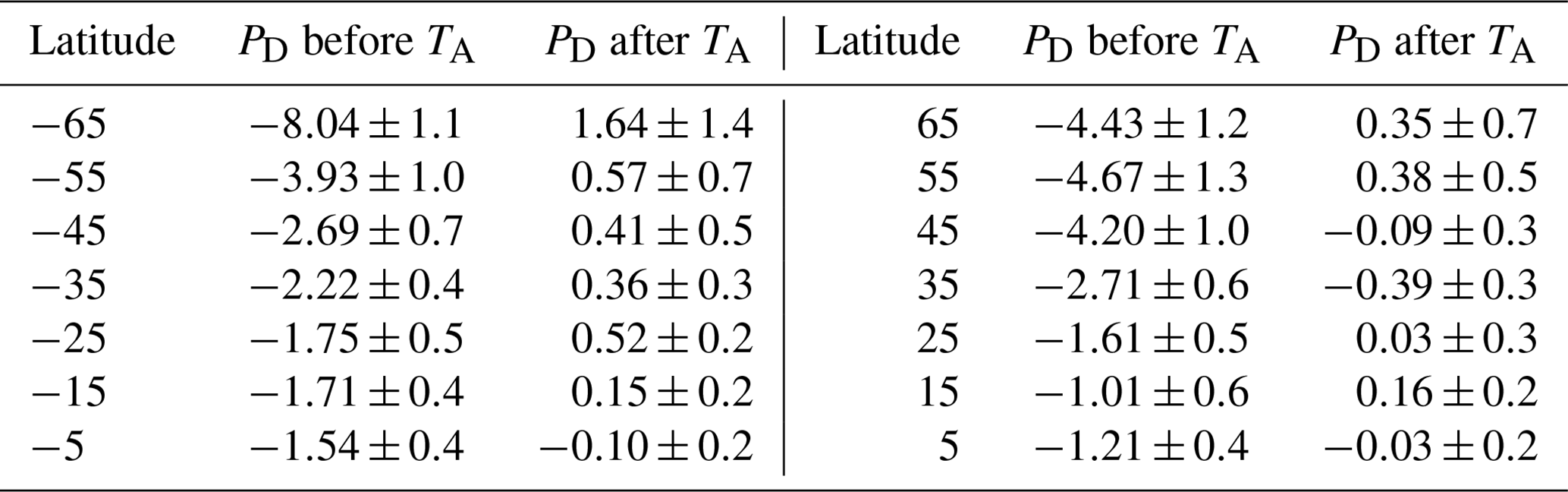
Monthly averaged total column ozone data (Ω_MOD(t,θ)) from the NASA Merged Ozone Data Set (MOD) were examined to show that the latitude-dependent (θ) ozone depletion turnaround dates (T_A(θ)) range from 1994 to 1998. T_A(θ) is defined as the approximate date when the zonally averaged ozone ceased decreasing. Ω_MOD data used in this study were created by combining data from Solar Backscattered Ultraviolet instruments (SBUV/SBUV-2) and the Ozone Mapping and Profiler Suite (OMPS-NP) from 1979 to 2021. The newly calculated systematic latitude-dependent hemispherically asymmetric T_A(θ) shape currently does not appear in the suite of chemistry–climate models that are part of the Chemistry–Climate Model Validation Activity (CCMVal), which combines the effects of photochemistry, volcanic eruptions, and dynamics in their estimate of ozone recovery. Trends of zonally averaged total column ozone in percent per decade were computed before and after T_A(θ) using two different trend estimate methods that closely agree, Fourier series multivariate linear regression and linear regression on annual averages. During the period 1979 to T_A(θ), the most dramatic rates of Southern Hemisphere (SH) ozone loss were $P_{\mathrm{D}}=-\mathrm{10.9}\pm \mathrm{3}$ % per decade at 77.5^∘ S and $-\mathrm{8.0}\pm \mathrm{1.1}$ % per decade at 65^∘ S, which is about double the Northern Hemisphere (NH) rate of loss of $P_{\mathrm{D}}=-\mathrm{5.6}\pm \mathrm{4}$ % per decade at 77.5^∘ N and 4.4±1 % per decade at 65^∘ N for the period 1979 to T_A(θ). After T_A(θ), there was an increase at 65^∘ S of $P_{\mathrm{D}}=\mathrm{1.6}\pm \mathrm{1.4}$ % per decade with smaller increases from 55 to 25^∘ S and a small decrease at 35^∘ N of $-\mathrm{0.4}\pm \mathrm{0.3}$ % per decade. Except for the Antarctic region, there only has been a small recovery in the SH toward 1979 ozone values and almost none in the NH.

1 Introduction

Ozone is a photolytically produced, photochemically destroyed, and dynamically distributed atmospheric gas that plays a crucial role in protecting the planet from harmful ultraviolet (UV) radiation from the sun. The atmospheric presence of bromine and the release of chlorine from the UV dissociation of synthetic chemicals, such as chlorofluorocarbons (CFCs), can break down the ozone layer at all latitudes. This is especially the case in the Antarctic region where heterogeneous chemistry on and within ice crystals and liquid droplets (Tritscher et al., 2021) in polar stratospheric clouds (PSCs) have a strong effect on the destruction of ozone during September and October (WMO, 2022; Tritscher et al., 2021; Solomon et al., 1986, 2016; Solomon, 1999; Crutzen and Arnold, 1986; Khosrawi et al., 2011). As the sun rises in spring, chemically active nitrogen oxides, chlorine, and bromine are released, causing the ozone hole to develop within the region enclosed by the polar vortex winds. The weak levels of sunlight are sufficient to initiate and maintain the catalytic ozone loss photochemistry. In November and December, the isolating polar vortex winds break down, and the Antarctic ozone hole region backfills by air exchange from southern midlatitudes, causing ozone depletion turnaround dates (T_A) (35–65^∘ S) to be delayed compared to the Northern Hemisphere (NH) midlatitudes. The recurring annual ozone hole event triggered international action to limit the production and use of ozone-depleting substances (ODSs) under the Montreal Protocol, which has been successful in reducing the emission of these substances, slowing down the depletion of the ozone layer globally and leading to a partial recovery in the Antarctic ozone hole region (Solomon et al., 2016; Strahan and Douglass, 2018). After the mid-1990s, several studies reported an increase in total column ozone (TCO), particularly in the midlatitudes to high latitudes of the Southern Hemisphere, as well as a reduction in the size and depth of the Antarctic ozone hole starting in the late 1990s (Solomon et al., 2016; Stone et al., 2018, 2021; Weber et al., 2022).

The cessation of ozone decrease was first observed in the mid-1990s when satellite data showed a stabilization and slight increase in ozone concentrations in the Antarctic ozone hole region. However, the recovery was not significant enough to be considered a trend at that time (Strahan and Douglass, 2018). In the early 2000s, further analysis of satellite and ground-based data showed that the rate of ozone depletion had slowed down. After the mid-1990s, the cessation of ozone depletion has been most evident in the Southern Hemisphere (SH) polar region, where ozone depletion had been most severe. Ozone recovery has been slow or non-existent at other latitudes. Recently, Weber et al. (2022) showed reduction in ozone at all latitudes prior to 1995 and reported positive statistically significant TCO trends from 1996–2020 at southern middle and high latitudes and over the SH polar cap in September. When dynamical terms were included in the regression, small positive trends were near the 2-standard-deviation 2σ threshold at northern midlatitudes and high latitudes, with no trend detected in the tropics or over the NH polar cap.

Despite the success of the Montreal Protocol (Velders et al., 2007), ozone concentrations continue to fluctuate, driven by natural and anthropogenic factors, such as changes in solar radiation, stratospheric circulation, global warming, and volcanic activity and changing emissions of ozone precursors (Dameris and Baldwin, 2012; Weber et al., 2022). The discussion by Dameris and Baldwin (2012) explored the possible effects of climate change on the dynamics of the atmosphere affecting ozone as ODSs change and particularly the change in the Brewer–Dobson circulation (Brewer, 1949; Dobson et al., 1926) that transports ozone from an upwelling in the equatorial region into the stratosphere and to downwelling into midlatitudes and high latitudes.

A comparison of several atmospheric chemistry and dynamics model studies as part of the Chemistry–Climate Model Validation Activity (CCMVal; Eyring and Waugh, 2010, their Fig. 1; Dhomse et al., 2018; Robertson et al., 2023) generally predicts an ozone turnaround date T_A in the year 2000 with no systematic latitude dependence. In particular, Robertson et al. (2023) show latitude dependence of long-term ozone recovery but T_A=2000 for all cases. Quoting from the SPARC Report No. 5 (Eyring and Waugh, 2010), “Common systematic errors in CCM results include: tropical lower stratospheric temperature, water vapor, and transport; response to volcanic eruptions”, which may affect the determination of T_A as a function of latitude and time. The results of this study may provide a convenient metric for model validation compared to T_A derived from ozone data.

This study will estimate new latitude-dependent ozone recovery dates or, more accurately, the dates of cessation of ozone decrease, T_A(θ) ranging from 1994 (equatorial region and 60–70^∘ N) to 1998 (60–80^∘ S). The calculated T_A(θ) and ozone trends (% per decade) include the effects of volcanic eruptions such as Mt. Pinatubo in 1991, dynamics, and atmospheric temperature changes. Ozone data used in this study are a subset of the Merged Ozone Data Set (MOD) Ω_MOD(t) (1970–2021) starting in 1979 with the Nimbus-7 SBUV (Solar Backscattered Ultraviolet) satellite instrument. From 1979 to 2021, the MOD was created by combining data from Solar Backscattered Ultraviolet instruments (SBUV/SBUV-2) and the Ozone Mapping and Profiler Suite (OMPS-NP). Methods of calculating trends from time series data are essential in the analysis of environmental and climate-related data. Here, we discuss two independent methods to estimate linear trends, (1) linear regression of annual averaged data and (2) Fourier time series decomposition or multivariate linear regression (MLR; Ziemke et al., 2019), which are discussed below. The two methods are compared and shown to give nearly identical results over their mutual latitude range of validity, 65^∘ S to 65^∘ N. The MLR method is not used in the regions poleward of the Arctic and Antarctic circles that have latitude-dependent extended winter polar night. The advantage of the MLR method (Eq. 1), or that in Weber et al. (2022), is that it can be used to estimate the effects of its individual components, while the annual average method can be used in the polar regions to estimate sunlit ozone trends where there is a latitude-dependent extended winter night.

2 The Merged Ozone Data Set (MOD)

Figure 1a shows the MOD zonally averaged Ω_MOD TCO data (Frith et al., 2014, 2020) set as a function of latitude (5^∘ latitude bands from 77.5^∘ S to 77.5^∘ N) and time (January 1979 to December 2021). Part of the Antarctic ozone hole (75 to 80^∘ S) is shown (blue color) and the high-latitude maxima, north and south (red color), with low values in the equatorial region. Figure 1b shows the 42-year zonally averaged and time-averaged ozone amounts and the maxima and minima annual envelopes as a function of latitude. Figure 1 shows the asymmetry in the monthly and zonally averaged ozone data between the hemispheres, with the Northern Hemisphere (NH) having more ozone than the Southern Hemisphere (SH) at corresponding latitudes. Part of the asymmetry is driven by the spring Antarctic ozone hole backfilling in the SH summer.

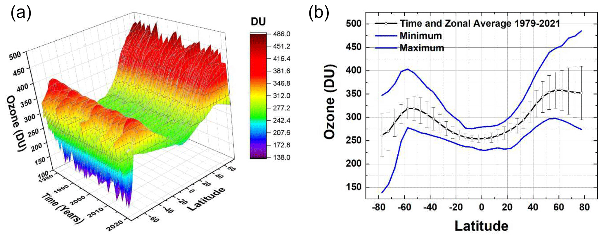
Figure 1 (a) The zonally and monthly averaged MOD data set 1979–2021 and −77.5 to 77.5^∘. (b) Time-averaged and zonally averaged ozone and its maxima and minima 1979–2021. Error bars are 1 standard deviation (±1σ).

Ω_MOD(t,θ) data provide a global view of ozone levels needed to track changes in ozone concentrations over time t for each latitude band θ. The SBUV and OMPS-NP series of satellite instruments form the longest (1979 to 2022) continuous global ozone Ω_MOD(t,θ) data record from a single instrument type. Merged ozone retrievals from the individual instruments use the version 8.7 retrieval algorithm (described by Weber et al., 2022) as an extension of the version 8.6 algorithm (Bhartia et al., 2013; McPeters et al., 2013; DeLand et al., 2012; Frith et al., 2017), specifically designed to improve cross calibrations between the later SBUV-type instruments in MOD starting from NOAA-16 in 2000. There were no external adjustments made to the ozone retrieval except for small high-altitude (>35 km) diurnal corrections to account for different measurement times between satellites and varying measurement time of day as individual satellite orbits slowly drift in Equator crossing time. These adjustments are very minor in TCO (Stacey Frith, personal communication, 2023). Data from each instrument are selected based on quality criteria outlined in Frith et al. (2014, 2020), and the data are averaged during periods when more than one instrument was operational. The Ω_MOD(t,θ) data are available as a function of latitude and month (https://acd-ext.gsfc.nasa.gov/Data_services/merged/, last access: 25 September 2023).

Analysis of the long-term ozone time series has been looked at extensively with references given in Weber et al. (2022). Methods for estimating trends from an oscillating time series with several distinct periodicities are well known (Ziemke et al., 2019; Stolarski et al., 1991, 1992; Herman et al., 1993). For ozone, one of the difficulties in trend estimation is that the early part of the time series shows a strong ozone decrease at all latitudes that continued until the mid-1990s and then flattens out and shows almost no recovery thereafter toward 1979 values. The Ω_MOD time series has been used extensively in ozone assessments and ozone depletion reports (e.g., WMO, 2022) and was recently compared to several other merged total ozone records in Weber et al. (2022). The validity of the Ω_MOD time series for estimating ozone trends was further checked (see Figs. A1 to A3 in Appendix A) in this study by showing detailed comparisons between the deseasonalized Ω_MOD time series with the deseasonalized MLS (Microwave Limb Sounder) overlapping stratospheric ozone time series (2005 to 2023).

3 Trend estimates from the MOD ozone data

Multivariate linear regression (MLR) is a Fourier-based method for analyzing atmospheric time series data that decomposes the time series into its component parts, including trend, quasi-biennial oscillation (QBO), solar cycle, ENSO (El Niño–Southern Oscillation), seasonality, and noise, resulting in a trend estimate and 2-standard-deviation 2σ uncertainty estimates (Ziemke et al., 2019). Calculated 2σ uncertainties for the MLR trends include a first-order autoregressive adjustment applied to the derived residuals (Weatherhead et al., 1998).

Linear trend estimates for the long-term changes in Ω_MOD(t,θ_i) globally and as a function of latitude θ_i have been obtained using the multivariate linear regression (MLR) model (e.g., Randel and Cobb, 1994, and references therein). The trend terms B(θ_i) were determined for Ω_MOD(t,θ_i) using Eqs. (1) and (2).

$$\begin{array}{}\text{(1)}& \begin{array}{rl}{\mathrm{\Omega }}_{\mathrm{MOD}}(t,{\mathit{\theta }}_i)& =\mathrm{A}\left({\mathit{\theta }}_{i}t\right)+\mathrm{B}({\mathit{\theta }}_i,t)\cdot t+\mathrm{C}({\mathit{\theta }}_i,t)\\ & \times {\mathrm{QBO}}_{\mathrm{1}}\left(t\right)+\mathrm{D}({\mathit{\theta }}_i,t)\times {\mathrm{QBO}}_{\mathrm{2}}\left(t\right)+\mathrm{E}({\mathit{\theta }}_i,t)\\ & \times \mathrm{ENSO}\left(t\right)+\mathrm{F}({\mathit{\theta }}_i,t)\times \mathrm{Solar}\left(t\right)+R(t,{\mathit{\theta }}_i),\end{array}\end{array}$$

where t is the month index (t=1 to 516 months with data for 1979–2021); A(θ_it) is the seasonal cycle coefficient; B(θ_i,t) is the trend coefficient; C(θ_i,t) is the first empirical orthogonal function (EOF) QBO coefficient and D(θ_i,t) the second EOF QBO coefficient, both representing the major components of the QBO variability; E(θ_i,t) is the ENSO coefficient; F(θ_i,t) is the solar cycle coefficient; and R(t) is the residual error time series. The F10.7 cm solar flux monthly time series is used for the Solar(t) proxy, the first and second leading EOF QBO monthly time series proxies QBO₁(t) and QBO₂(t) are used for the QBO component (Wallace et al., 1993), and Niño 3.4 (Oldenborgh et al., 2021) is used for ENSO(t) (Niño 3.4: https://www.ncei.noaa.gov/access/monitoring/enso/sst, last access: 25 September 2023). QBO₁(t) and QBO₂(t) are nearly orthogonal (correlation coefficient approximately zero) oscillating time series based on data with approximately a 2.3-year periodicity. A(θ_i,t) involves seven fixed constants, while B(θ_i,t) (and all other remaining coefficients) involves five fixed constants for each θ_i. The harmonic expansion for A(t) (similar for the other coefficients) is

$$\begin{array}{}\text{(2)}& \begin{array}{rl}\mathrm{A}\left(t\right)=& a\left(\mathrm{0}\right)+\sum _{p=\mathrm{1}}^{\mathrm{3}}\left[a\right(p\left)\cos \right(\mathrm{2}\mathit{\pi }pt/\mathrm{12})\\ & +b\left(p\right)\sin (\mathrm{2}\mathit{\pi }pt/\mathrm{12})],\end{array}\end{array}$$

where a(p) and b(p) are constants. Statistical uncertainties for A(t) and B(θ_i) were derived from the calculated statistical covariance matrix involving the variances and cross-covariances of the constants (e.g., Guttman et al., 1982; Randel and Cobb, 1994).

In this study the locally weighted scatterplot smoothing (Lowess(f)) least-squares technique is used to reduce oscillations in the time series data and to estimate T_A(θ) where f is the fraction of data averaged together (Cleveland, 1979; Cleveland and Devlin, 1988).

The latitude average residual R(t) in percent of the MOD ozone amount $(\mathrm{100}\langle R(t,{\mathit{\theta }}_i)/{\mathrm{\Omega }}_{\mathrm{MOD}}(t,{\mathit{\theta }}_i)\rangle )$ is shown in Fig. 2 for the SH and NH as an indication of how well Eq. (1) is able to fit the Ω_MOD(t,θ_i) time series.

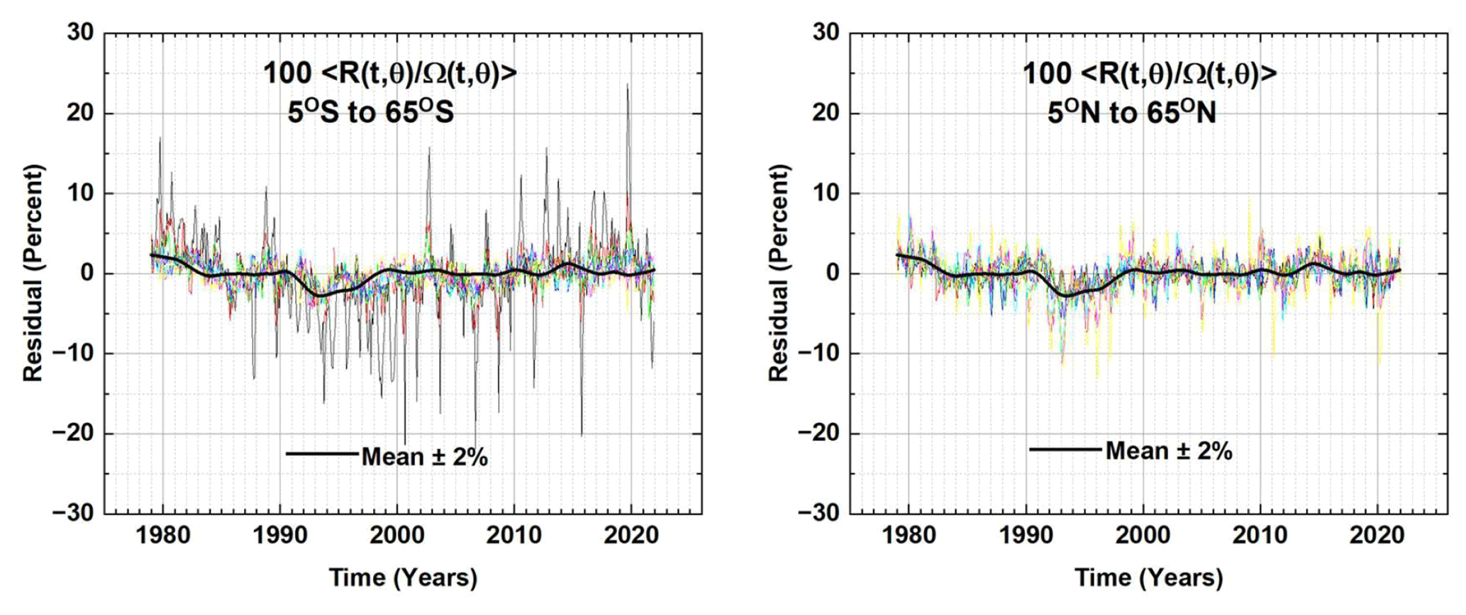
Figure 2 The latitude average residual term from Eq. (1) in percent of $\mathrm{100}\langle R(t,q_i)/W_{\mathrm{MOD}}(t,q_i)\rangle$. The black line is the Lowess(0.1) fit (Cleveland, 1979) to the R(t,q) with an average error estimate of ±2 %. The light-colored lines are each latitude's R(t,q) in a hemisphere 0^∘ $<\mathit{\theta }<$ 65^∘.

The SH R(t,θ) is more variable than the NH, with the largest variations arising in the 55 and 65^∘ S latitude bands. On average, Eq. (1) fits the original data Ω_MOD(t,θ_i) to within ±2 %.

The linear deseasonalized trend results B(θ_i) are obtained for 14 latitude bands θ_i (centered on 65^∘ S to 65^∘ N). The latitudinal trends P_D(θ_i) are expressed in percent per decade, given by Eq. (3), where the denominator D is either the time average 〈Ω〉 of the area-weighted global ozone average (Fig. 1) or the time average $D\left({\mathit{\theta }}_i\right)=\langle {\mathrm{\Omega }}_{\mathrm{MOD}}(t,{\mathit{\theta }}_i)\rangle$ for each latitude band over the considered period. The whole-year period considered is 1979–2021.

$$\begin{array}{}\text{(3)}& P_D\left({\mathit{\theta }}_i\right)=\mathrm{1000}\mathrm{B}\left({\mathit{\theta }}_i\right)/\mathrm{D}\left({\mathit{\theta }}_i\right)\left(\mathit{\%}\text{per decade}\right)\end{array}$$

In the second method, the trend is estimated using annual integrals (annual averages) that remove the seasonality and other short-term oscillations but ignore longer-term oscillations such as the 28- to 29-month QBO cycle and the average 11.3-year solar cycle. A comparison of the two trend-estimating methods is shown in Fig. 3 for the entire 1979 to 2021 period showing that they agree quite closely but that the annual average method has slightly larger 2-standard deviation 2σ thresholds than the MLR method.

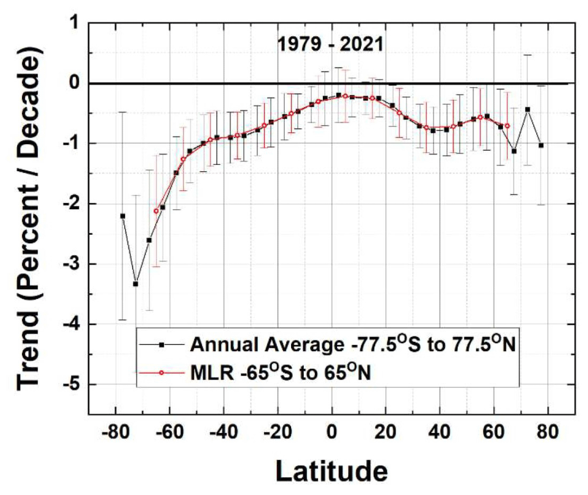
Figure 3 The ozone trend P_D(θ) for the entire period 1979–2021 for two methods, MLR and annual average. The latitude grids for the two methods are offset to show the agreement in the trends and 2σ error bars.

The MLR method (Eqs. 1 and 2) is not applied poleward of the Arctic and Antarctic circles where latitude-dependent extended winter night periods occur. Additional latitude-dependent terms of varying periods would be needed for latitudes greater than 70^∘. The annual average method does not have these complications.

The Fig. 3 estimation of linear long-term trends since 1979 is misleading, since ozone showed significant annual declines until the mid-1990s and then increased slightly thereafter, meaning the average long-term time series is non-linear. The usual procedure is to determine linear trends separately before and after the turnaround dates T_A (Weber et al., 2022). However, as is shown later, there is no single turnaround date applicable to all the latitudes between 80^∘ S and 80^∘ N. Instead, there is a range spanning 1994 to 1998.

Figure 4a shows the Ω_MOD time series for 5^∘ S and 5^∘ N and Fig. 4b the deseasonalized and smoothed (Lowess(0.05)) Ω_MOD time series. After deseasonalizing but not removing QBO effects (Eq. 1), both the 2.3-year QBO oscillation and the reduced ozone effects from volcanic eruptions are shown in Fig. 4b. Some volcanos (e.g., from El Chichón, March 1982; Mt. Pinatubo, June 1991; and Manaro Voui, July 2018) inject significant amounts of SO₂ into the lower stratosphere, leading to the formation of aerosols that reduce UV light and the production of ozone, especially in the equatorial region.

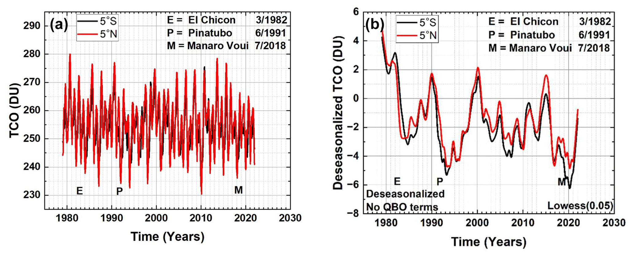
Figure 4 (a) Ω_MOD time series for θ=5^∘ N and 5^∘ S. (b) The deseasonalized TCO time series for θ=5^∘ N and 5^∘ S without removing QBO effects (Eq. 1). The approximate dates are shown of volcanic eruptions that injected large amounts of SO₂ into the stratosphere, leading to minima approximately 1 year later.

Figure 5 shows the Lowess(0.3) fits (black curves) to the Ω_MOD data for four sample latitude bands (55^∘ S, 45^∘ S, 55^∘ N, and 45^∘ N) that track the longer-term changes in the Ω_MOD time series. Also shown are examples of f=0.1 (red) and f=0.05 (blue dots). The Lowess(0.05) fit (blue dots) shows considerable structure with a minimum in 1993 that is likely related to the Mt. Pinatubo eruption and a modest El Niño effect in 1991–1992. The estimated values of T_A for f=0.1 and 0.05 can differ by 6 months from those determined when f=0.3 because of short-term oscillations. The Lowess(0.3) degree of smoothing removes most of the short-term effects on ozone such as QBO and those from volcanic eruptions from El Chichón (1982) and Mt. Pinatubo (1991), both well before the earliest estimated T_A in 1994.

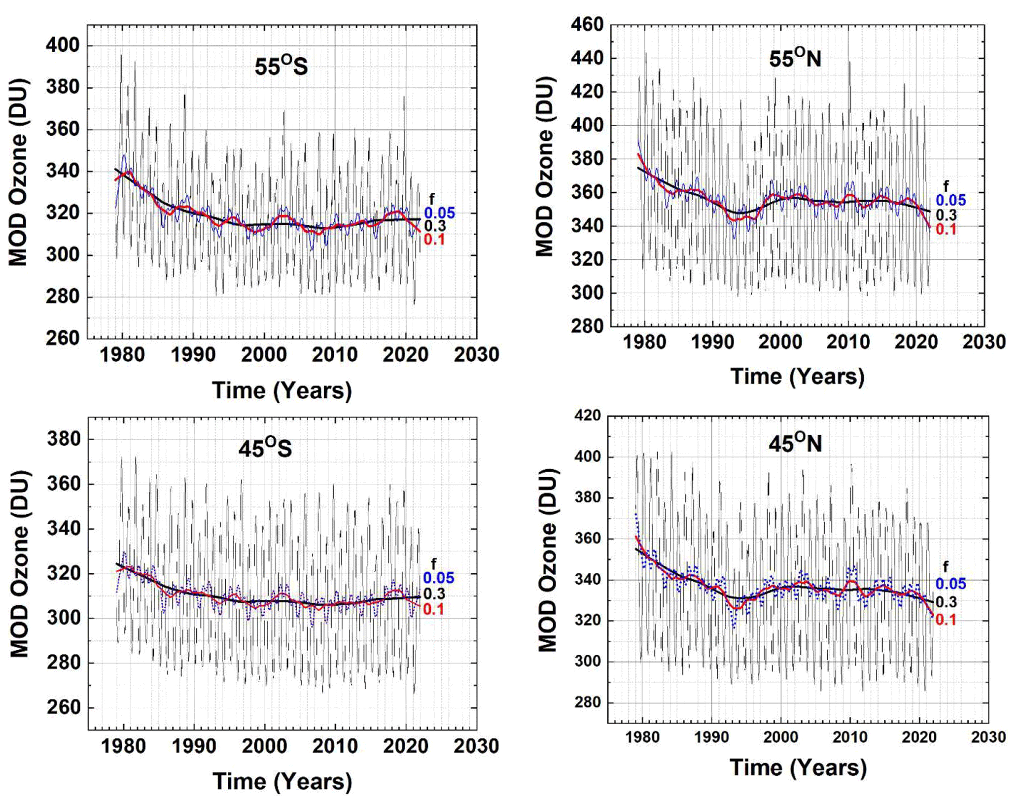
Figure 5 Ω_MOD in four latitude bands and Lowess(0.3) fitting functions (f=0.3, black lines). Examples of different f=0.1 (red) and 0.05 (blue dots) are shown at 45^∘ S and 45^∘ N. Note the slight downturn since 2010 in the Lowess(0.3) at 45 and 55^∘ N.

Figure 6 shows the Lowess(0.3) fits to the Ω_MOD data (1979 to 2021) for 16 latitude bands, −75^∘ $<\mathit{\theta }<$ 75^∘ on an expanded ozone scale. Each of the Lowess(0.3) plots for the various latitudes shows different periods of ozone decrease and subsequent turnaround T_A(θ) after the mid-1990s. Use of expanded ozone scales appears to show a sharp downturn after 2010 at some latitudes (25 to 75^∘ N). As shown later, the apparent downturns in the Lowess(0.3) fit to Ω_MOD after 2010 are not yet statistically significant in trend estimates from Ω_MOD as an indicator of long-term ozone decrease.

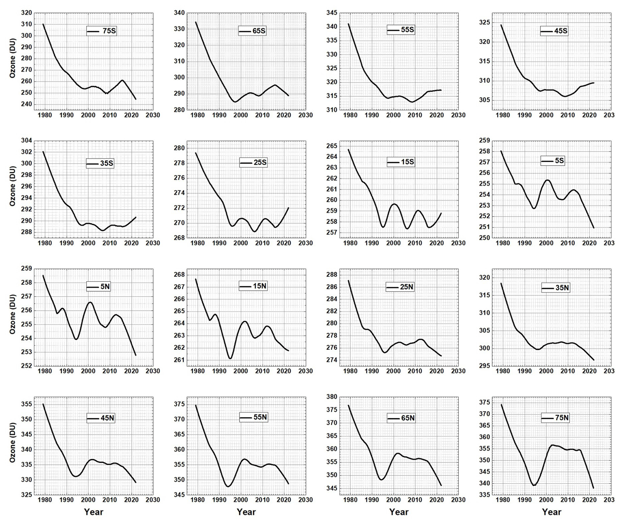
Figure 6 Lowess(0.3) fits to the Ω_MOD data for 16 latitude bands used to determine T_A(θ). Note that the ozone scale varies for each latitude.

Figure 7 shows the turnaround dates T_A(θ) that are obtained by taking the first derivatives of Fig. 6 data and finding the zero-crossing time corresponding to the appropriate minimum value in Fig. 6. The exact turnaround dates determined have a precision of ±0.1 years and an accuracy of ±0.5 years. The ±0.5 uncertainty does not affect the calculation of trends before and after the estimated T_A(θ). What is interesting is that some of the turnaround dates in Fig. 7 are separated by over 4 years and are strongly asymmetric between the hemispheres. Figure 7 shows a near symmetry for early turnaround dates 1994–1996 for low latitudes between ±25^∘ that corresponds to the Brewer–Dobson ozone upwelling region (Brewer, 1949; Dobson et al., 1926; Butchart, 2014) where most of the ozone is created by sunlight and then transported poleward. At poleward latitudes, the turnaround dates are quite different, with a delayed date, 1997, at high SH latitudes (35–65^∘ S) and 1998 at 75^∘ S compared to 1994 at high NH latitudes (45 to 75^∘ N).

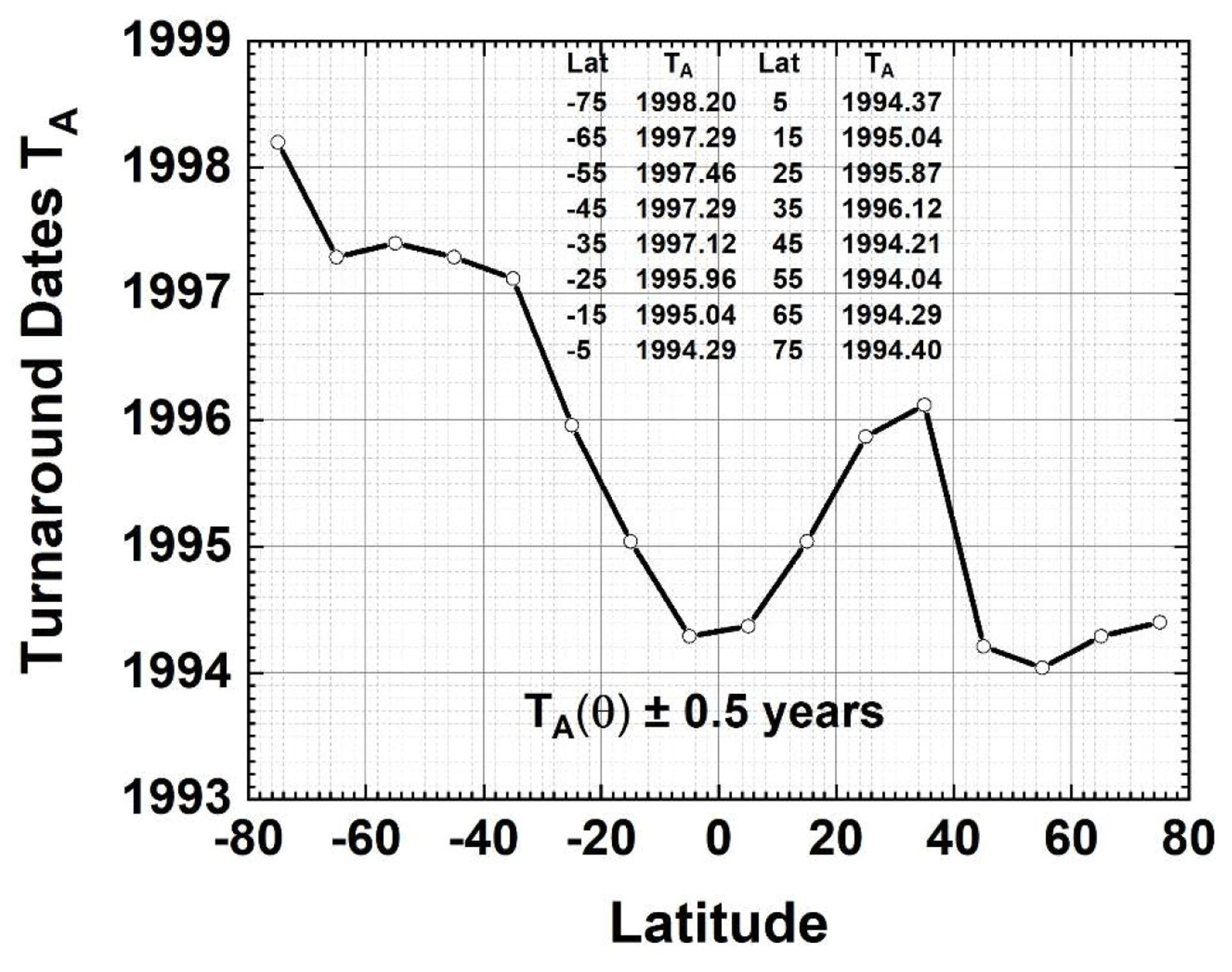
Figure 7 Turnaround dates T_A(θ) as a function of latitude from Fig. 6 with an estimated accuracy of ±0.5 years based on the analysis in Fig. 5.

The T_A delay to 1997 for latitudes 35–65^∘ S follows the delayed recovery of ozone depletion within the spring Antarctic ozone hole (Solomon, 1999; Stone et al., 2021, their Fig. 3; Bodeker and Kremser, 2021, their Figs. 6 and 9) and backfilling (air exchange with lower-latitude ozone-rich air) during the summer months after the polar vortex winds break down in October–November.

The general T_A(θ) pattern shown in Fig. 7 should appear in model calculations as a signature of the combined effects of photochemistry, dynamics, and volcanic eruptions on the cessation of decreasing ozone in the mid-1990s.

Trends (linear slopes) P_D(θ) in percent per decade are estimated (Eq. 3) for the separate periods before and after T_A(θ) in each latitude band (Fig. 8) and for the entire period (Fig. 3). The linear slopes obtained by the two methods, MLR and annual average, closely agree (Figs. 3 and 8) with the annual average method extended to polar latitudes (Fig. 8a). Table 1 contains the data from Fig. 8a and b.

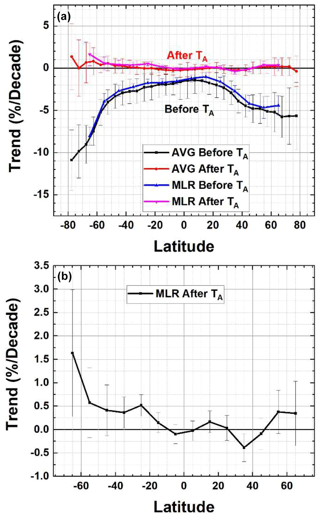
Figure 8 (a) Ozone trends P_D(θ) (percent per decade) using the MLR and annual average methods before and after T_A(θ). (b) A magnified version of the MLR estimated trends after T_A with 2σ uncertainties.

Table 1 MLR trends (% per decade) ±2σ.

The latitude-dependent trends derived by Weber et al. (2022), using 1996.5 as the approximate T_A (their Fig. 3), agree within error bars with the trends shown in Fig. 8 for all latitudes, but they suggest T_A=2000 for the polar regions. The trends also agree within error bars with those in WMO (2022). As mentioned earlier, the trend estimates are not very sensitive to the exact T_A, but the shape of T_A(θ) should be a model validation marker contained in model calculations for all effects, not just ODSs.

The delayed (1997) Southern Hemisphere midlatitude and high-latitude values of T_A are caused by coupling to the increasing Antarctic spring ozone loss after 1979 until a recovery starting in about 1998–2000 (Solomon et al., 2016). The midlatitude and high-latitude delay, from 35 to 65^∘ S, is caused by the summer mixing of ozone-poor air from the Antarctic region with SH midlatitude ozone-rich air once the polar vortex winds break down in November–December.

The asymmetry between the Arctic and Antarctic is caused by the lower winter Antarctic temperatures (−80 ^∘C), leading to the formation of low-altitude clouds containing ice crystals along with the isolating Antarctic polar vortex winds (Solomon et al., 2007, 2016). In the spring sunlight, the ice and water droplets (Tritscher et al., 2021) release ODSs and deplete ozone to a monthly average of about 155 DU. During the summer, air exchange with ozone-rich air from lower latitudes comes into the polar latitudes and fills in the ozone layer above Antarctica (monthly average about 300 DU). Smaller but significant ozone losses occurred in the Arctic region, caused by occasional low temperatures and ODSs. The Arctic does not routinely have the low temperatures needed for winter ice clouds, nor does it have the persistent isolating polar vortex winds because of wave action forced by the land topography. The latitude band at 75^∘ N (Fig. 1) has the highest amount of monthly average winter ozone, 450±25 DU, that decreases to 290±20 DU monthly average during the summer, comparable to midlatitude values. The result is earlier values of T_A in the NH compared to the SH. The NH T_A is earlier than the 1997 minimum in stratospheric halogens (Weber et al., 2022; Newman et al., 2007). Note that T_A is not the time of the start of recovery but rather the time for the end of rapid ozone decrease.

Before the SH T_A, total column ozone decreased at a rate of $P_{\mathrm{D}}=-\mathrm{10.9}\pm \mathrm{3.6}$ % at 77.5^∘ S and $-\mathrm{8.0}\pm \mathrm{1.1}$ % per decade at 65^∘ S, during the period from 1979 to 1997, with smaller decreases from 55 to 25^∘ S (Fig. 8a). After the turnaround period T_A, ozone at 65^∘ S increased at $P_{\mathrm{D}}=\mathrm{1.6}\pm \mathrm{1.4}$ % per decade based on the MLR method. After T_A, most other latitudes (Fig. 8b) show stationary ozone amounts within 2σ. In the NH the decreases were smaller than in the SH before T_A because of the absence of an Arctic ozone hole region. At 77.5^∘ N, the decrease was $P_{\mathrm{D}}=-\mathrm{5.6}\pm \mathrm{4}$ % per decade and at 65^∘ N $P_{\mathrm{D}}=-\mathrm{4.4}\pm \mathrm{0.35}$ % per decade.

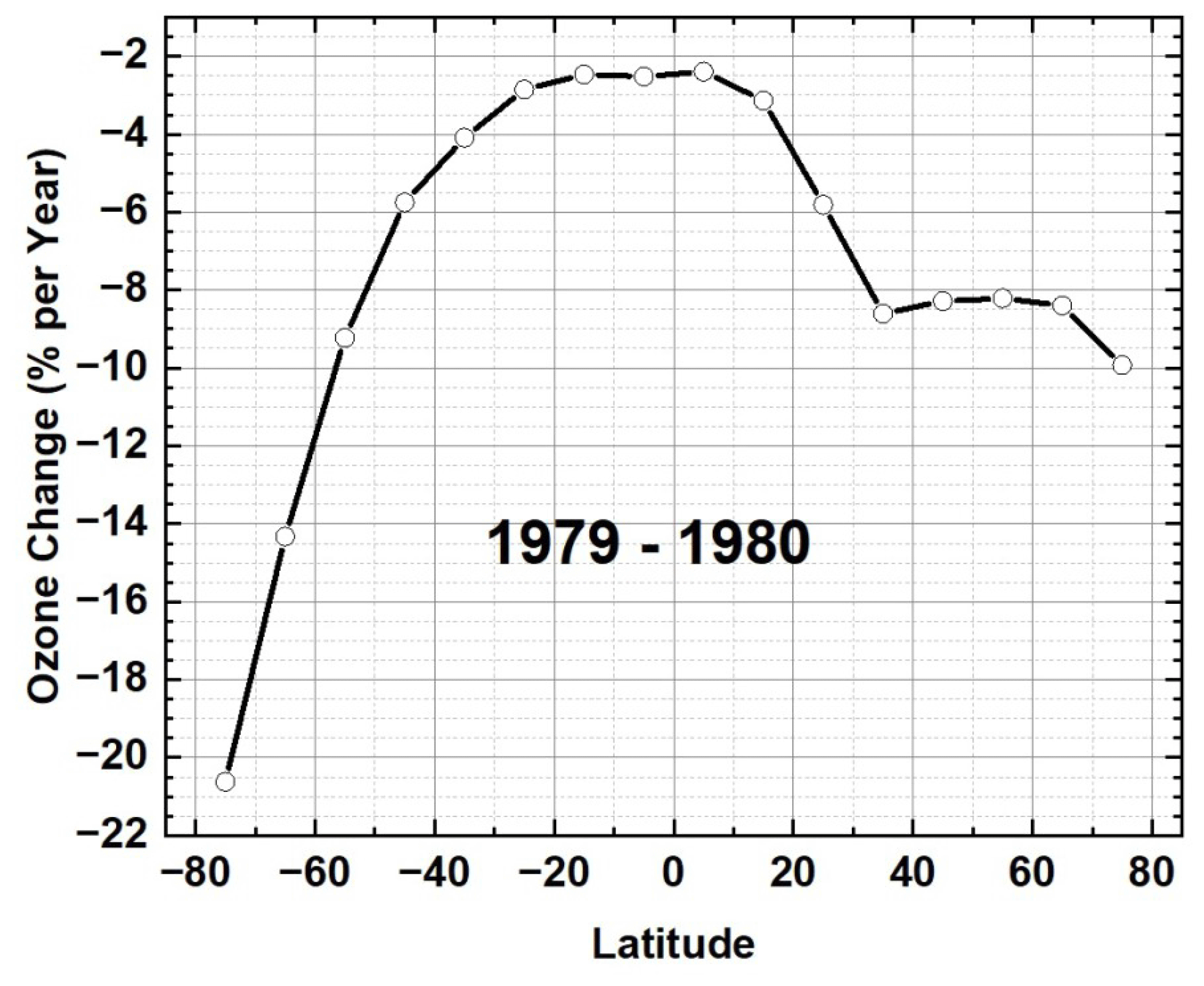
An analysis of ozone trends prior to the start of reliable satellite data in late 1978 showed that the annual rate of ozone loss (% yr⁻¹) increased after 1978 (Staehelin et al., 2001). Based on the first derivatives of the data in Fig. 6, the maximum annual rate of ozone reduction occurred in 1979 and 1980 in the NH and SH (Fig. 9) except for 65^∘ N in 1992, where the rate of loss is −8.75 % yr⁻¹. The loss rates range from −20.6 % yr⁻¹ at 75^∘ S to 2.39 % yr⁻¹ at 5^∘ N. A smaller loss rate occurred for 35 to 75^∘ N, where the loss rate is almost constant between 8 and 10 % yr⁻¹ compared to the larger SH loss rates caused by the presence of the springtime Antarctic ozone hole.

Figure 9 The percent change in ozone per year in 1979 and 1980.

The Lowess(0.3) plots in Fig. 6 suggest that Ω_MOD has been declining since approximately 2010 from 5^∘ S to 65^∘ N but still increasing from 45 to 65^∘ S (Fig. 6). However, computing the trends (Fig. 10) from Ω_MOD(t,θ) using either the MLR (Eq. 1) or annual average methods suggests that the declines in ozone from 25^∘ S to 65^∘ N are not yet significant at the 2σ level over the period 2010–2021.

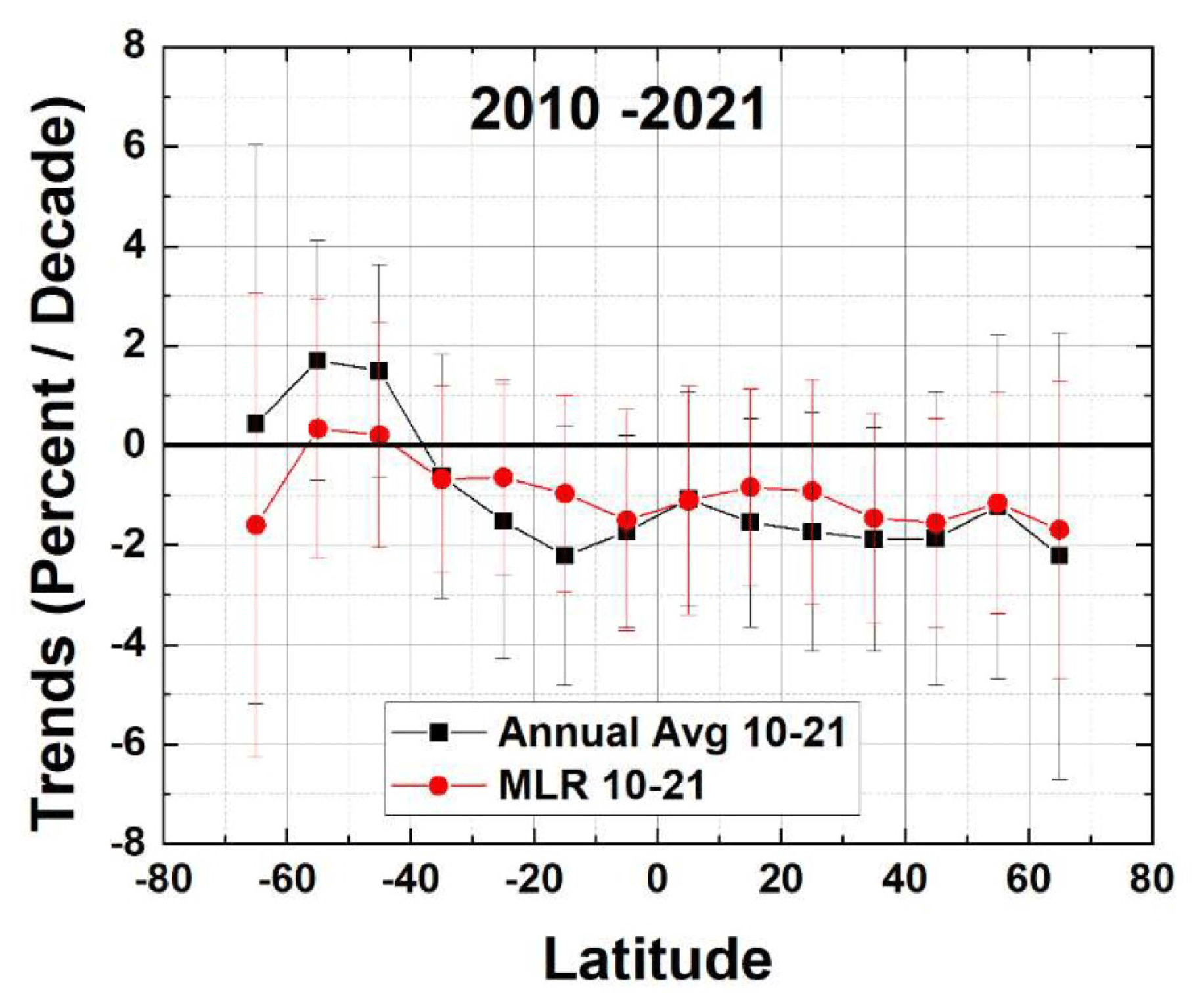
Figure 10 Ozone trends P_D(θ) (percent per decade) for the period 2010–2021 for the annual average and MLR methods applied to Ω_MOD(t,θ).

Comparing deseasonalized Ω_MOD(t,θ) with deseasonalized Microwave Limb Sounder (MLS; see Figs. A1–A3 in Appendix A) stratospheric ozone from 2005 to 2021 shows small average (Lowess(0.3)) differences that are within ±1 DU except for 2021, when the differences at both 65^∘ S and 65^∘ N are about −2.5 DU. This suggests that the calibrations of the later SBUV-2 and OMPS-NP instruments are stable. For 2016 to 2018, Ω_MOD is obtained from NOAA-19 SBUV and OMPS-NP and from just OMPS-NP since 2018. Figure A3 suggests that there was a decrease in tropospheric ozone in 2020 that may correspond to reduced economic activity during the COVID-19 pandemic.

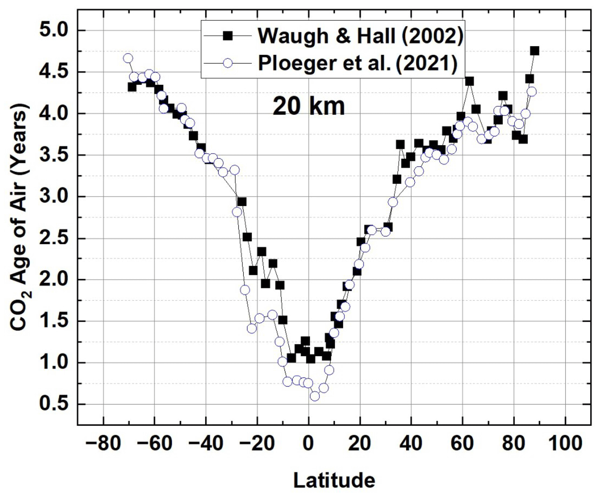
Age of air (AoA) is a measure of how long a parcel of air resides in the stratosphere after it leaves the troposphere (Linz et al., 2016; Ploeger et al., 2021). A comparison of T_A with AoA estimates from the relatively inert tracer gas CO₂ (Fig. 11) for the altitude range near the ozone maximum (approximately 20 km) vs. latitude (based on Waugh and Hall, 2002, their Fig. 6a and Ploeger et al., 202, their Fig. 10a) shows near symmetry between the hemispheres, with the shortest AoA in the equatorial region. The turnaround dates T_A in Fig. 6 are also symmetric in the equatorial zone, corresponding to the upwelling Brewer–Dobson circulation and the smaller AoA. This suggests that the combined effects of chemistry and dynamics on ozone amounts are similar between ±25^∘. The precursors to ODSs are also lifted into the equatorial stratosphere and transported towards the polar regions (Newman et al., 2004, 2007), where they can be photo-dissociated into ODSs. Ozone at higher latitudes, NH and SH, with longer AoA, will be dependent on transported ozone and ODSs and their photochemistry and especially the different dynamics and chemistry in the Arctic and Antarctic regions.

Figure 11 Age of air derived from CO₂ data (Waugh and Hall, 2002; Ploeger et al., 2021).

4 Summary

The monthly averaged Merged Ozone Data Set Ω_MOD values (2.5^∘ latitude bands, 77.5^∘ S to 77.5^∘ N) from 1979 to 2021 were averaged into 10^∘ latitude bands 75^∘ S $<\mathit{\theta }<$ 75^∘ N. A smoothed Ω_MOD version based on Lowess(0.3) was used to determine the approximate dates of the latitude-dependent end-of-ozone decrease date T_A(θ) ranging from 1994 to 1998, with an error estimate of ±0.5 years. The systematic hemispherically asymmetric latitude-dependent pattern T_A(θ) should appear in atmospheric models that combine the effects of volcanic eruptions, photochemistry, and dynamics in their estimate of the end of ozone decrease. An examination of model studies that are part of CCMVal shows a nearly uniform T_A=2000, suggesting that several models' chemistry and dynamics including volcanic effects are incomplete. The hemispheric asymmetry is caused by the formation of the annual spring Antarctic ozone (monthly spring average about 155 DU) hole with persistent isolating polar vortex winds followed by the summer mixing with midlatitude ozone-rich air (December average about 300 DU). The Arctic region does not form a large spring ozone hole, nor does it have sustained isolating polar vortex winds. Instead, at 75^∘ N (Fig. 1), it has the highest amount of monthly average winter ozone (450±25 DU) that decreases to a 290±20 DU monthly average during the summer. Trends of ozone P_D(θ) in percent per decade were computed before and after the latitude-dependent T_A(θ) using two different methods, MLR and annual averages, that closely agree over their mutual latitude range of validity, 65^∘ S to 65^∘ N. The annual average method can extend into polar latitudes. The most dramatic rates of ozone loss were $P_{\mathrm{D}}=-\mathrm{10.9}\pm \mathrm{3.6}$ % per decade at 77.5^∘ S and $-\mathrm{8.0}\pm \mathrm{1.1}$ % per decade at 65^∘ S, which is about double the rate of loss of $P_{\mathrm{D}}=-\mathrm{5.7}\pm \mathrm{4}$ % per decade at 77.5^∘ N and $-\mathrm{4.4}\pm \mathrm{1.2}$ % per decade at 65^∘ N. During the period after T_A to 2021, there has been a small increase at latitudes in the SH from 25 to 65^∘ S, with the largest value being 1.6±1.4 % per decade at 65^∘ S. Aside from the small increases in the SH region there has been no statistically significant ozone recovery toward 1979 values, just an almost constant ozone amount after T_A(θ). The largest annual rate of ozone decrease occurred near the beginning of the SBUV data record, 1979, showing large high-latitude losses of −20.6 % yr⁻¹ at 75^∘ S, caused by the springtime Antarctic ozone hole, compared to a smaller Arctic loss of −9.9 % yr⁻¹ at 75^∘ N. During the period 2010 to 2021, there was a small apparent decrease in ozone amount in Ω_MOD that is not yet statistically significant at the 2-standard-deviation level. A comparison between Ω_MOD and MLS stratospheric column ozone shows small systematic negative differences in 2020 that mostly recovered in 2021, except near the Equator. This suggests that there is no statistically significant instrumental calibration drift between Ω_MOD TCO and MLS stratospheric ozone.

Appendix A

The MOD TCO data record since 2018 is obtained from OMPS-NP, which appears to show decreasing TCO (Fig. 6). Because of this, the deseasonalized Ω_MOD data are compared with MLS (Microwave Limb Sounder) deseasonalized stratospheric column ozone for the period 2004 to 2021 to look for calibration drifts in the Ω_MOD time series. The question addressed here is not the absolute agreement between Ω_MOD and the MLS mostly stratospheric ozone column but rather if there is a systematic drift between the two data sets after 2016. Figures A1 and A2 show the difference between the two deseasonalized time series for latitudes from 65^∘ S to 65^∘ N and for the entire period 2005–2021. Of interest is the period 2016 to 2021, when Ω_MOD was derived using NOAA-19 SBUV and OMPS-NP 2016–2018 and from OMPS-NP since 2018.

The differences in Figs. A1 and A2 between Ω_MOD and MLS since 2016 are not statistically significant at the 2σ level. Variations of ±3 DU are within the Ω_MOD merged record uncertainties.

Since both MOD and MLS time series were deseasonalized, the mean values would be zero, unless there were changes in tropospheric ozone or instrument calibration drift. The differences are summarized in Fig. A3, along with the 2σ^′ (σ^′ is the standard deviation from the mean) error bars estimated from the average of each deseasonalized time series. In 2020 there appears to be a systematic change in 〈MOD−MLS〉 that may be a reduction in tropospheric ozone amount of about 3 DU, caused by the economic slowdown associated with COVID-19 (Ziemke et al., 2022). The systematic change mostly recovered in 2021 (Fig. A3) except for −1 DU near the Equator (−5^∘ S to 15^∘ N).

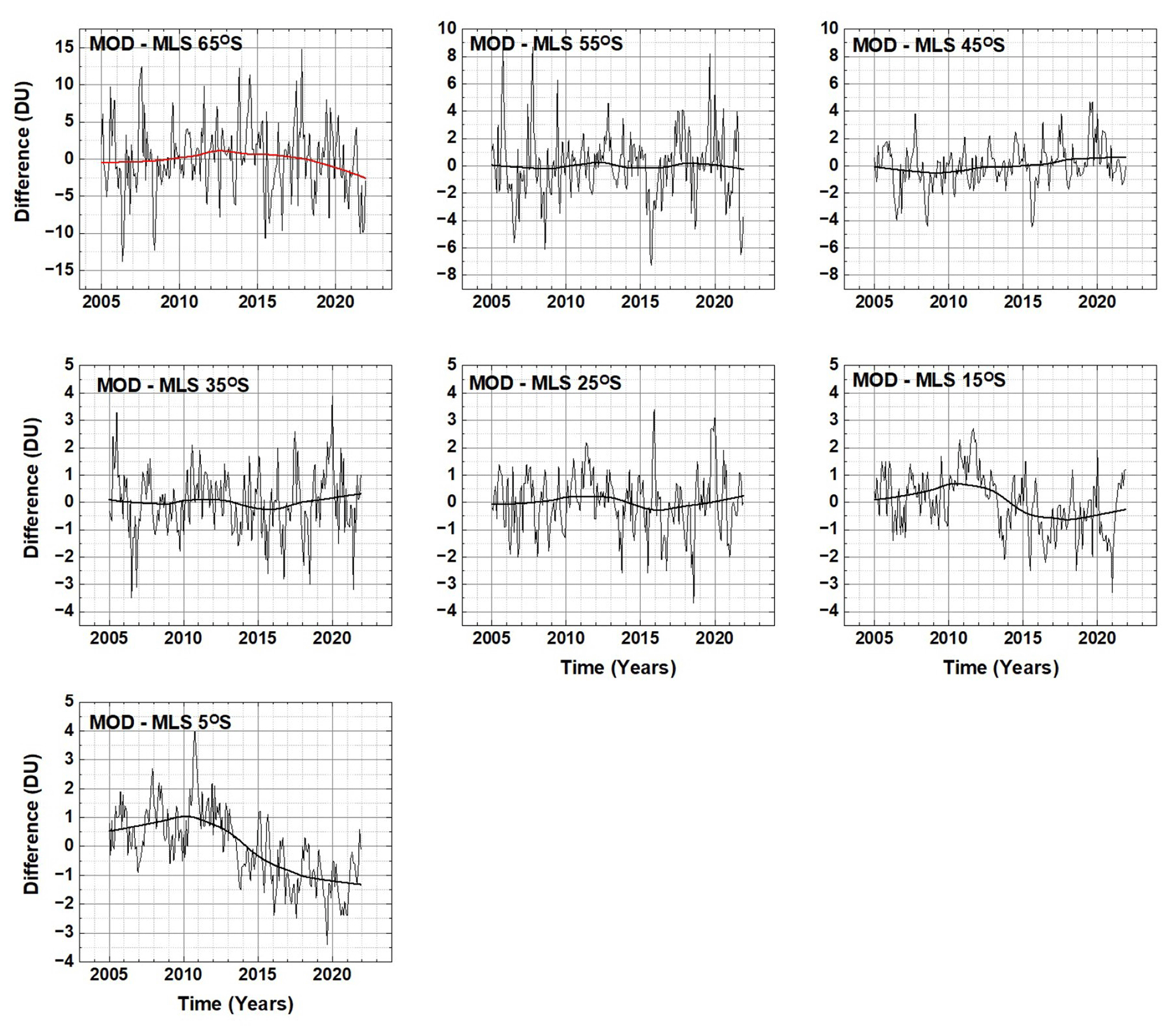
Figure A1 A comparison of deseasonalized Ω_MOD with deseasonalized MLS stratospheric column ozone for 65 to 5^∘ S.

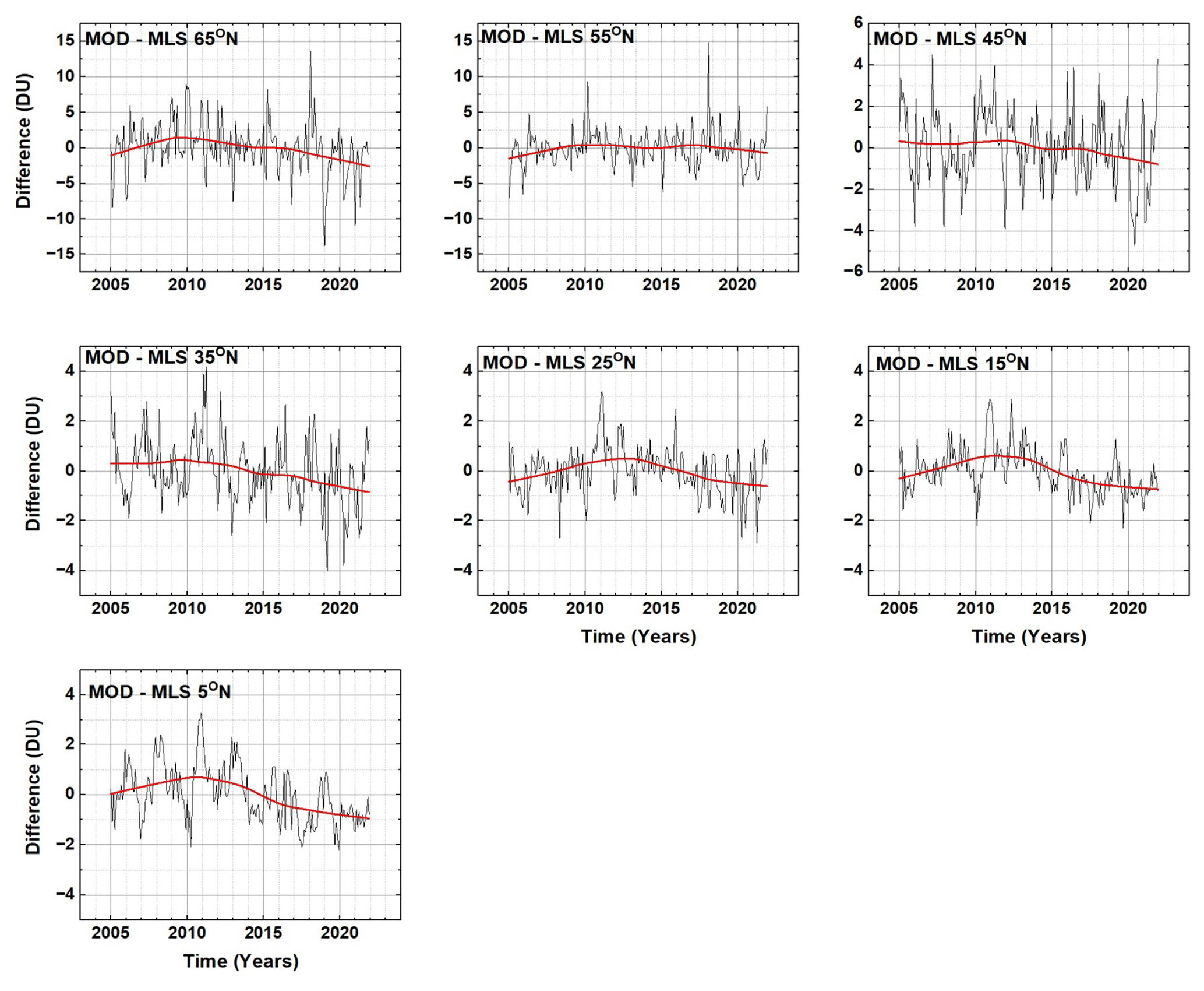
Figure A2 A comparison of deseasonalized MOD total ozone with deseasonalized MLS stratospheric column ozone for 5 to 65^∘ N. Variations of ±3 DU are within the MOD merged record uncertainties.

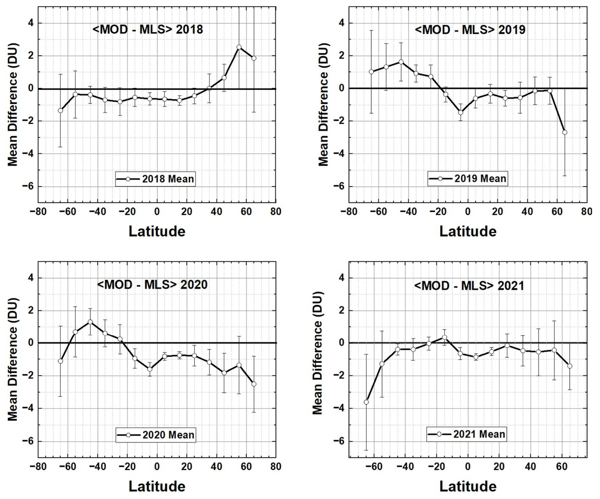
Figure A3 Annual average 〈MOD−MLS〉 for the years 2018 to 2021. Error bars are 2σ^′, where σ^′ is the standard error of the mean estimated from the average of the deseasonalized time series for each year shown in Figs. A1 and A2.