the Creative Commons Attribution 4.0 License.
the Creative Commons Attribution 4.0 License.
 | 27 Oct 2023
A comparative analysis of in situ measurements of high-altitude cirrus in the tropics
Martina Krämer
Armin Afchine
Guido Di Donfrancesco
Luca Di Liberto
Sergey Khaykin
Lorenza Lucaferri
Valentin Mitev
Max Port
Christian Rolf
Marcel Snels
Nicole Spelten
Ralf Weigel
Stephan Borrmann
We analyze cirrus cloud measurements from two dual-instrument cloud spectrometers, two hygrometers and a backscattersonde with the goal of connecting cirrus optical parameters usually accessible by remote sensing with microphysical size-resolved and bulk properties accessible in situ. Specifically, we compare the particle backscattering coefficient and depolarization ratio to the particle size distribution, effective and mean radius, surface area density, particle aspherical fraction, and ice water content. Data were acquired by instruments on board the M55 Geophysica research aircraft in July and August 2017 during the Asian Monsoon campaign based in Kathmandu, Nepal, in the framework of the StratoClim (Stratospheric and upper tropospheric processes for better climate predictions) project. Cirrus clouds have been observed over the Himalayan region between 10 km and the tropopause, situated at 17–18 km. The observed particle number densities varied between 10 and 10−4 cm−3 in the dimensional range from 1.5 to 468.5 µm in radius. Correspondingly, backscatter ratios from 1.1 up to 50 have been observed.
Optical-scattering theory has been used to compare the backscattering coefficients computed from the measured particle size distribution with those directly observed by the backscattersonde. The aspect ratio of the particles, modeled as spheroids for the T-matrix approach, was left as a free parameter to match the calculations to the optical measures. The computed backscattering coefficient can be brought into good agreement with the observed one, but the match between simulated and measured depolarization ratios is insufficient. Relationships between ice particle concentration, mean and effective radius, surface area density, and ice water content with the measured backscattering coefficient are investigated for an estimate of the bulk microphysical parameters of cirrus clouds from remote sensing lidar data. The comparison between particle depolarization and aspherical fraction as measured by one of the cloud spectrometers equipped with a detector for polarization represents a novelty since it was the first time the two instruments were operated simultaneously on an aircraft. The analysis shows the difficulty of establishing an univocal link between depolarization values and the presence and amount of aspherical scatterers. This suggests the need for further investigation that could take into consideration not only the fraction of aspheric particles but also their predominant morphology.
- Article
(17573 KB) - Full-text XML
- BibTeX
- EndNote


Cirrus are high clouds that exist between −35 and −85 ∘C. They are composed of ice crystals of micron to millimeter size (Lynch et al., 2002), and they are fairly widely dispersed, usually resulting in relative transparency and whiteness and often producing halo phenomena not observed with other cloud forms (AMS, 2023). Higher elevations of cirrus are usually found in the tropics, where their highest occurrence frequency is also recorded, and lower elevations are found in polar regions (Sassen et al., 2008, 2009). Tropical cirrus originate either from outflows from deep convective clouds (liquid-origin cirrus) or from vertical uplifting of air (in situ-origin cirrus) associated with Kelvin or gravity waves, as well as with the synoptic-scale tropospheric tropical ascent (Jensen et al., 1996; Pfister et al., 2001; Immler et al., 2008; Fujiwara et al., 2009; He et al., 2012; Krämer et al., 2016; Luebke et al., 2016; Wernli et al., 2016). Studies of these clouds are important for a better understanding of their impact on the climate as they play a crucial role in Earth’s radiation budget (Prabhakara et al., 1993; Campbell et al., 2016; Lolli, 2017; Krämer et al., 2020). Their impact is based on two effects (Stephens, 2002, 2005): (i) a greenhouse potential that traps the outgoing longwave radiation emitted by the Earth and the atmosphere underneath and (ii) their albedo that reflects the incoming solar radiation. The balance between the cirrus-induced warming and cooling depends on their coverage, height, thickness, and horizontal and vertical temperature distributions, as well as the ice crystal size and shape distributions within the clouds (Lynch, 1996; Boucher et al., 2013). Moreover, cirrus are an essential modulator of the water budget in the upper troposphere and in the stratosphere (Luo et al., 2003; MacKenzie et al., 2006; Corti et al., 2008; Fueglistaler et al., 2009).
The qualitative and quantitative assessments of the cirrus properties over large spatial and temporal scales require the use of satellite data. Methods exist to provide spaceborne retrievals of cirrus bulk and microphysical parameters. Passive visible or thermal, spectrally resolved measurements have been used to infer the cloud optical depth, ice particle effective radius (Reff) and ice water path (Meyer and Platnick, 2010; Sourdeval et al., 2013; Guignard et al., 2012; Sourdeval et al., 2015) but may subsample clouds of small optical thickness. Active remote sensing by radars and lidars can be more sensitive to thin clouds and can still provide information on cirrus geometrical and optical properties with high spatial and temporal resolutions. Vertical profiles of cirrus extinction, ice water content (IWC) (for definitions of abbreviations used throughout the text, please refer to the “List of abbreviations” in the Appendix) and Reff are retrieved using lidar and/or radar measurements (Austin et al., 2009; Delanoë and Hogan, 2010). Global mapping of cirrus properties is obtained from satellite-borne instruments like the CALIOP (Cloud and Aerosol Lidar with Orthogonal Polarization) lidar aboard the CALIPSO (Cloud-Aerosol Lidar and Infrared Pathfinder Satellite Observation) polar-orbiting satellite (Nazaryan et al., 2008). Such measurements have begun to include estimates of ice crystal number concentrations (Nice). In fact, climate model parameterizations of ice cloud optical properties are based on Reff and IWC (Fu, 2007), but these two do not fully constrain the ice cloud particle size distribution (PSD) and its optical properties (Mitchell et al., 2011). Moreover, the knowledge of Nice on a global scale would ameliorate the understanding of ice nucleation and its parameterization in climate models. A refinement of the ice crystal nucleation rates would in turn improve the predictions of Reff. Mitchell et al. (2018) use co-located observations from the Infrared Imaging Radiometer (IIR) and from CALIOP to retrieve Nice, Reff and IWC in semi-transparent cirrus clouds, while Sourdeval et al. (2018) employ combined lidar–radar measurements to provide satellite estimates of Nice using a methodology that constrains moments of a parameterized particle size distribution (PSD) through lidar extinction and radar reflectivity.
Cirrus clouds' microphysical properties have been characterized by in situ measurements taken during several airborne observation campaigns (Thomas et al., 2002; Schiller et al., 2008; Krämer et al., 2009; Frey et al., 2011; Luebke et al., 2013; Frey et al., 2014; Krämer et al., 2016; Schumann et al., 2017). A review of these studies and of the challenges they present is reported in Baumgardner et al. (2017), while Krämer et al. (2020) describe extensive statistics of meteorological parameters, IWC, Nice, ice crystal mean radii (Rmean) and relative humidities with respect to ice and water vapor mixing ratios from airborne in situ measurements performed during 150 flights over 24 campaigns in the mid-latitudes and the tropics. Such observational activity, in addition to being essential for shedding light on the processes of formation, aging and dissipation of the clouds, is of great help in the interpretation of satellite sensor data, allowing the calibration and validation of the retrievals of cirrus microphysical and bulk parameters by comparing them with the corresponding results of in situ measurements.
In the present work, we intend to compare optical measurements of cirrus clouds, i.e., particle backscatter coefficient β and total particle depolarization δTA, with bulk and microphysical parameters observed by cloud spectrometers and hygrometers. The optical measurements are generally accessible to lidar probing, but in our case, they have been taken in situ by a backscattersonde; henceforth, they are directly comparable with the other data acquired in situ as all measurements originate from the same air parcel. Measurements were taken during the aircraft field campaign of the EU-funded project StratoClim (Stratospheric and upper tropospheric processes for better climate predictions), carried out in southern Asia in 2017. A full description of the campaign is provided by Stroh et al. (2023). The southern Asian campaign of the high-altitude research aircraft M55 Geophysica (Stefanutti et al., 1999) focused on detailed observations of atmospheric transport and physical–chemical processes which dominate the input of air and aerosols into the (sub-)tropical stratosphere.
In the present work, we make use of data from seven flights performed on 29 and 31 July and on 2, 4, 6, 8 and 10 August 2017. During these flights, the airplane penetrated cirrus clouds several times for nearly 6 h of observations in clouds over approximatively 35 flight hours. Most of the measurements during StratoClim were performed at temperatures <205 K, corresponding to potential temperatures > 355 K and altitudes > 14 km, i.e., in the TTL. Krämer et al. (2020) report a description of the clouds observed during the campaign. The first part of the campaign period suffered from very rare cloud passes at elevated altitudes, with comparatively low cloud particle number concentrations (below 1 cm−3). In fact, during this period, the vast majority of clouds were encountered during ascent from or during approach to Kathmandu Airport. On 29 and 31 July and on 2 August, most of the clouds were come across at a pressure level of ∼ 400 hPa (and higher) during ascent and descent, with cloud particle concentrations ranging from 100 to 1000 cm−3. The second campaign period (flights on 4, 6, 8 and 10 August 2017) provided extended fields of cirrus clouds of convective origin, with elevated particle densities and broad size distributions covering almost the entire detection size range of the different particle probes. The cloud particle measurements, mostly carried out over the southern slopes of the Himalayas, captured high ice water content up to 2400 ppmv and ice particle aggregates exceeding 700 µm in size. The observed ice particles were mainly of liquid origin, with only a small amount formed in situ. ERA5 reanalysis corroborates the presence of high IWC detrained from deep-convective clouds. A microphysical modeling study by Lamraoui et al. (2023) focuses on the flight of 10 August, but its results can probably also be applied to the other cases of convectively generated cirrus measured during the second part of the campaign. The study predicts ice habits and reproduces the observed IWC, ice number concentration and bimodal ice particle size distribution. The lower range of particle sizes is mostly represented by planar and columnar habits, while the upper range is dominated by aggregates with sizes between 600 and 800 µm. The study suggests that most of the measured ice particles are of liquid origin, with only a small amount formed in situ. The latter are associated with low values of IWC and number concentration, which makes them less influential in regulating the IWC, which is, on the contrary, substantially influenced by planar ice particles of liquid origin. The difference in ice number concentration across habits can be up to 4 orders of magnitude, with aggregates occurring in much smaller numbers.
We verify the ability and limits of optical modeling in reproducing the results of remote sensing optical measurements from the concomitant in situ microphysical ones, thus assessing the compatibility of the two datasets. Closure studies between aerosol light-scattering coefficients and aerosol PSD with optical modeling are common in atmospheric science, and they often use measurements from in situ nephelometers and Mie theory applied to particle spectrometer data (Wex et al., 2002; Teri et al., 2022). Similar approaches have also been attempted by comparing lidar or backscatter probe measurements with cloud spectrometers mounted on balloons or on airplanes in the characterization of polar stratospheric clouds (Schreiner et al., 2002; Deshler et al., 2000; Scarchilli et al., 2005; Snels et al., 2021; Cairo et al., 2023). Comparatively fewer studies compare the size distributions of ice crystals in cirrus clouds and their modeled and measured optical scattering properties; this is particularly true for backscattering measurements (Wagner and Delene, 2022). The reason probably lies in the greater difficulty of obtaining significant and definitive confirmations from such optical closures. This is likely because of the uncertainties that affect both the particle size distribution measurements and their optical modeling and that arise from the large dimensional range of the ice crystals, extending for more than 3 orders of magnitude, and the great variety of shapes that they can take simultaneously within the cloud (Bailey and Hallett, 2009). A further complication arises from the presence of rough irregular surfaces, corners and edges in ice crystals (Schnaiter et al., 2011). Actually, modeling of the optical properties of cirrus clouds is a formidable problem that probably does not always have a valid solution despite the numerous methods available for calculating scattering from aspherical particles (Mishchenko et al., 1999; Konoshonkin et al., 2017a). In fact, many light-scattering computation methods have been employed to calculate the scattering properties of cirrus particles, and we may quote the finite-difference time domain (FDTD) method (Sun et al., 1999), the discrete dipole approximation (DDA) (Yurkin et al., 2007), the boundary element method (Groth et al., 2015), the pseudo-spectral time domain method (Liu et al., 2012), the surface integral equation method (Nakajima et al., 2009) and geometrical optics in various implementations: the improved geometric optics method (IGOM) (Yang and Liou, 1996a), the geometric optics integral equation (GOIE) (Ishimoto et al., 2013) and the ray-tracing geometric optics method (GOM) (Macke et al., 1996). The T-matrix theory offers a solution to the computation of electromagnetic scattering from axisymmetric particles and has practical advantages over other methods, largely due to its analytical character and the exploitation of particle symmetries, which considerably simplifies the calculation and has long been used to study the scattering properties of cirrus clouds. Mishchenko et al. (1997) used it to compute the backscattering from horizontally oriented ice platelets in cirrus; Baran et al. (2001) modeled the absorption and extinction properties of the finite hexagonal ice columns and plates in random and preferred orientations; Liu et al. (2006) reported results for the scattering properties of small cirrus crystals modeled as mixtures of polydisperse, randomly oriented spheroids and cylinders with varying aspect ratios; and Bi and Yang (2014) employed it to compute the optical properties of randomly oriented ice crystals of various shapes, including hexagonal columns, hollow columns, droxtals, bullet rosettes, and aggregates. T-matrix theory has also been used to simulate the response of cloud spectrometers with forward-scattering geometries when exposed to clouds of aspherical particles (Borrmann and Luo, 2000).
Finally, the possibility of using microphysical observations taken along with optical observations usually accessible in remote sensing but here obtained with quasi in situ techniques (the air mass sampled by the backscattersonde is, for all practical purposes, the same as that sampled by hygrometers and cloud spectrometers) allows us to establish relationships between β; δTA; and cloud parameters retrieved from the measured PSDs such as Nice, Rmean, Reff, Surface area density (SAD), particle aspherical fraction (AF), and cloud IWC, with the latter being retrieved from a comparison of data from hygrometers that differentially measure the proportion of gaseous and total water. These empirical relationships are useful in interpreting lidar measurements of cirrus clouds in terms of their microphysical and bulk parameters.
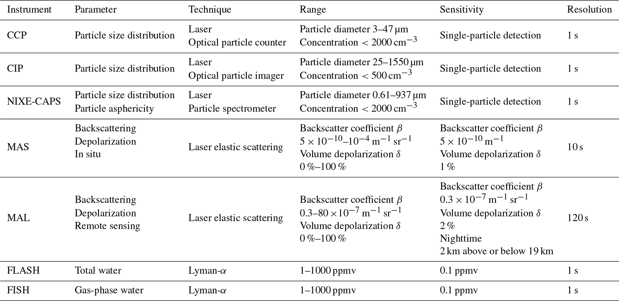
We have compared and used data from the two dual-instrument cloud spectrometers that flew aboard the aircraft Geophysica, the NIXE-CAPS and the CCP. Both instruments (see Sect. 2.2) are developments of droplet measurement technologies (DMTs) and are nearly identical in their technology, the sensors used for pressure and temperature, and the flow measurement technology (Prandtl's pitot tube system). The IWC has been derived from the total water hygrometer FISH and the water vapor hygrometer FLASH (see Sect. 2.3); the cloud backscattering coefficient and depolarization ratio at 532 nm have been derived from the in situ backscattersonde MAS (see Sect. 2.1). Data from MAS are also compared in some cases of interest with the 532 nm elastic lidar MAL.
2.1 Particle backscatter measurements: MAS and MAL instruments
2.1.1 The MAS backscattersonde
Optical observations in situ have been provided by the backscattersonde MAS, which is basically a polarization diversity Rayleigh lidar that measures in situ the same parameters accessible to lidars. It is located in a bay beneath the pilot's cockpit, facing sideways on the right. It emits polarized laser light at 532 nm and collects the light backscattered from the portion of atmosphere that is in close proximity (3–10 m) to the instrument, sensitive to air molecules, cloud particles, and aerosols. Polarization-resolved observations allow us to detect the particle's asphericity and, hence, thermodynamic phase. The sampling volume is approximately 10−3 m−3; the resolution is 10 s, corresponding to a 1.5–1.9 km horizontal resolution along the aircraft trajectory, given the 154±39 m s−1 aircraft speed at altitude (Weigel et al., 2021a, b).
The backscattered light is split into two channels according to polarization, allowing the measurement of the backscatter ratio (BR) and the volume depolarization δ, the particle depolarization δA, and the total particle depolarization δTA. These optical parameters follow the usual definitions (Cairo et al., 1999) reported here for convenience; the subscripts mol and A denote, respectively, the molecular and particle contribution to the measured parameters, and cross and par denote the perpendicular and parallel polarization of the backscattering coefficient β (Collis and Russell, 1976).
Note the different definitions of particle depolarization δA and total particle depolarization δTA, which will both be used in the following. To pass from one to the other definition, please refer to Cairo et al. (1999).
The signal detected in the parallel (cross) channel is directly proportional to . The BR is derived by a calibration procedure that uses collocated measurements of pressure and temperature to retrieve the air density and defines a suitable constant K – taking into account the molecular scattering cross-section, as well as the instrumental sensitivity – in order to achieve BR =1 in air masses where no particles are present. A description of the instrument and data processing can be found in Cairo et al. (2011).
Figure 1 reports the 2D histogram of the frequency distribution of BRs with respect to geometrical altitude; the cloud observations are clustered in two regions, namely between 7.5 and 10 km and above 13 km up to the tropopause region, with the cold-point tropopause being at 17 km on average. In the following, we will focus on observations made in that upper region. We identify cloud presence when BR >1.2.
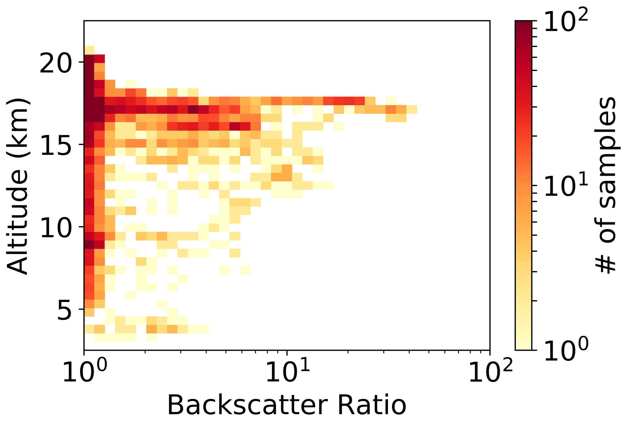
Figure 1A 2D histogram of backscatter ratio vs. altitude. Data were acquired throughout the campaign by the MAS backscattersonde. The color codes indicate the number of observations in the 2D bin, representing 8477 data points.
Figure 2 exhibits δTA with respect to temperature for clouds observed above 11 km. In the upper part of the troposphere, i.e., when temperatures fall below 200 K, a negative trend with respect to temperature can be discerned; in that altitude range, an increase in δTA with altitude has often been reported for cirrus (Sassen and Benson, 2001; Sunilkumar and Parameswaran, 2005; Cairo et al., 2021). However, at higher temperatures, namely at around 205 and 215 K, observations of highly depolarizing clouds are also reported. To avoid contamination by aerosols or an excessive uncertainty in the depolarization for very low BRs, we will restrict our analysis to observations with BR >1.2 for a total of 2132 data points.
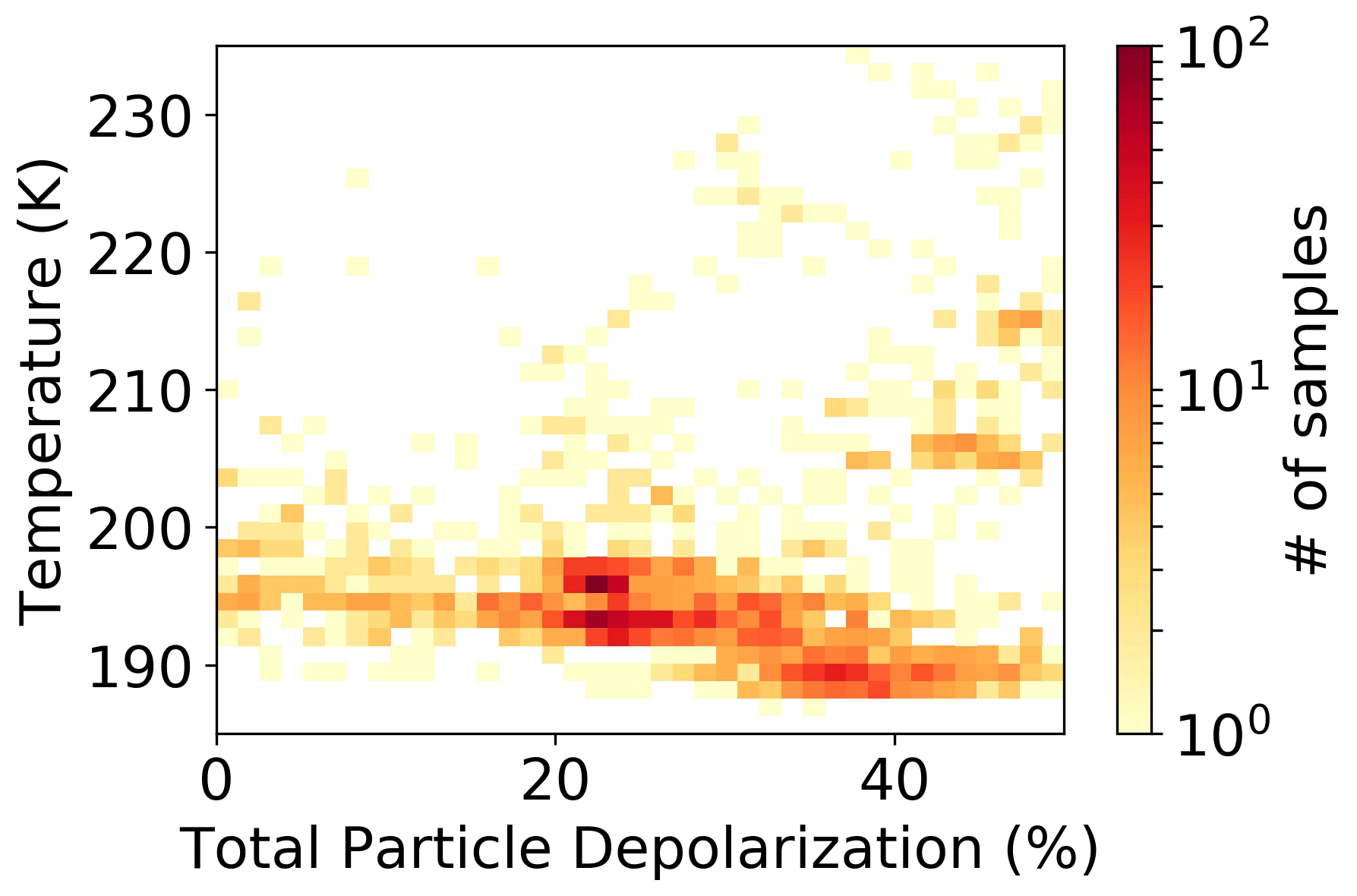
Figure 2A 2D histogram of total particle depolarization data vs. temperature for altitudes above 11 km. Data were acquired throughout the campaign by the MAS backscattersonde. The color codes indicate the number of observations in the 2D bin, representing 2308 data points.
2.1.2 The MAL lidars
The lidars MAL1 and MAL2 (Miniature Aerosol Lidars Mk1 and Mk2) are depolarization diversity Rayleigh lidar instruments operating at 532 nm (Martucci et al., 2005). They use micropulse lasers with pulse repetition rates of 4.5–5.5 kHz. MAL1 is installed on M55 Geophysica for upward probing, while MAL2 is for downward probing. The measured parameters are BR and δ. The definitions of the measured and processed parameters follow Eqs. (1)–(5). The high repetition rate combined with the low pulse energy of the laser allows the use of a photon-counting detection–acquisition system with high dynamic range. This makes it possible to start the lidar profile as close to the aircraft as allowed by the geometrical overlap function, i.e., at 400 m from the platform, delivering backscatter and depolarization profiles every 2 min, with a vertical resolution of 50 m. The processing procedure is based on a comparison of the signal from the clouds with the molecular backscatter signal from aerosol-free parts of the lidar profile. In this, it is similar to the one for MAS, except that in MAL, the particle-free atmospheric volumes are identified in the lidar profile at some range above and below the aircraft and not at the flight altitude. The lidars participated in a number of campaigns with M55 Geophysica (Cairo et al., 2004; Molleker et al., 2014; Mahnke et al., 2021). This includes a comparison case with the CALIPSO lidar CALIOP during the RECONCILE campaign (Mitev et al., 2012).
2.2 Cloud spectrometers
2.2.1 The NIXE-CAPS instrument
The NIXE-CAPS (for details see Luebke et al., 2016; Costa et al., 2017) is located below the aircraft wing and incorporates two instruments: the CAS-DPOL (Cloud and Aerosol Spectrometer with detector for polarization) and the NIXE-CIPgs (Cloud Imaging Probe gray scale); it also includes an air speed sensor and a temperature probe. CAS-DPOL is a light-scattering probe covering the particle size range of 0.3 to 25 µm in radius. Moreover, it records the change of polarization in the backward-scattered light, thus giving information about the particle asphericity.
NIXE-CIPgs is an optical-array probe that covers the particle size range between 7.5 and 468.5 µm. The instrument captures the image of a cloud particle by using a 64-element photodiode array (15 µm resolution) to generate two-dimensional shadow images that can be analyzed for particle size and asphericity using various algorithms (Costa et al., 2017).
For aircraft speeds between 240 and 80 m s−1, the instruments' sampling volumes limit the particle concentration measurements to concentrations above 0.02 to 0.05 cm−3 (NIXE-CAS-DPOL) and about 0.0001 to 0.001 cm−3 (NIXE-CIPgs).
The particle size distributions (PSDs) of CAS-DPOL and CIPgs are merged into a single PSD covering the range of 0.3 to 468.5 µm, where the size bins up to 20 µm are taken from the CAS-DPOL, and those larger than 20 µm are taken from the CIPgs. This threshold is used since the CIPgs has a larger sampling volume than the CAS-DPOL, thus providing better particle-sampling statistics. Particles larger than 1.5 µm in radius are classified as cloud, while the smaller particles are considered to be aerosols.
The PSDs are reported for each second. In the present work, the PSDs have been averaged over 10 s and synchronized to the backscattersonde data. In the following, in addition to the PSD, we have used the combined aspherical fraction AFi, which refers to the fraction of aspherical particles detected in size channels from both NIXE-CAS and NIXE-CIPgs. The AFs are derived as described by Costa et al. (2017)
In order to study its relationship with the microphysical measurements, we have used the mean AF defined as follows:
2.2.2 The CCP instrument
The CCP (Cloud Combination Probe) combines a CDP (Cloud Droplet Probe) with a CIPgs (Cloud Imaging Probe with gray scale), whose measurement technique and data analysis have been described in detail (Frey et al., 2011; Molleker et al., 2014; Klingebiel et al., 2015; Grulich et al., 2021). The CCP-CDP is a light-scattering probe comparable to the CAS-DPOL (or NIXE-CAS), but it covers the range of 2.5–46 µm in particle diameter with a size resolution of 1–2 µm (Mei et al., 2020), also encompassing the uppermost range of the aerosol size spectrum. The sampling area of the CCP-CDP was examined by Klingebiel et al. (2015), yielding 0.27±0.025 mm2 with an uncertainty of less than 10 %. In contrast, the CCP-CIPgs is an optical-array probe designed to detect cloud particles and hydro-meteors with a resolution of 15 µm. CIPgs captures images of cloud particles using a 64-element photodiode array to obtain two-dimensional images with nominal detection diameters ranging from 15 to 960 µm. CCP-CDP and NIXE-CAS performances have been frequently validated by glass-sphere calibrations. Before or after each flight, CCP-CIPgs and NIXE-CIP calibrations were performed using spinning disks carrying opaque spots sized to the particle range to be detected. Particle concentration data measured with CCP are corrected for compression under measurement conditions using a thermodynamic approach developed by Weigel et al. (2016).
2.3 FISH and FLASH hygrometers
The FISH (Fast In situ Stratospheric Hygrometer) instrument is a closed-path Lyman-α photo-fragment fluorescence hygrometer (Zöger et al., 1999; Meyer et al., 2015) used to measure H2Otot in the range of 1–1000 ppmv between 50 and 500 hPa with an accuracy and precision during StratoClim of 7 % and 0.3 ppmv. FISH is calibrated versus a reference frost-point mirror, MBW 373 LX, on the ground before and after each flight to ensure high data quality. On board Geophysica, the inlet for the H2Otot hygrometer FISH is mounted on the side of the aircraft, is heated, and has a 90∘ bend to quickly evaporate ice crystals. In the present work, the original 1 s resolution data have been averaged over 10 s.
FLASH (FLuorescent Airborne Stratospheric Hygrometer; for details, see Khaykin et al., 2013, 2022) also uses the Lyman-α photo-fragment fluorescence technique for the detection of water vapor, but its inlet is designed to sample only the gas phase. The detection range is 1–1000 ppmv, with an accuracy and precision of <9 % and 0.5 ppmv. The time resolution is 1 Hz; here, data have been averaged over 10 s. The H2Ogas hygrometer FLASH is mounted below the wing and equipped with its own inlet.
Clear-sky data from the two hygrometers have been intercompared together and with those from a third hygrometer on board the M55 Geophysica, ChiWIS (Chicago Water Isotope), designed for airborne measurements of vapor-phase water isotopologues in the dry upper troposphere–lower stratosphere with integrated cavity output absorption spectroscopy (Sarkozy et al., 2020). The comparison showed excellent agreement between these in situ instruments (Singer et al., 2022).
Table 3 summarizes the main features of the instruments used in this study.
We first compare the particle backscattering computed from the measured PSD, namely βNIXE−CAPS, with the β measured by the backscattersonde MAS. We then present regressions between the particle backscattering coefficient β and particle number density Nice, the mean radius Rmean, the effective radius Reff, SAD, and IWC. We will assume that the dispersion of the data in the comparison could be used as an estimate of the uncertainty to be attributed to such regressions. In addition, we investigate the relation of the particle aspherical fraction (AF) with the measured total particle depolarization δTA and with other cloud microphysical and environmental parameters.
3.1 Optical modeling
The backscattering coefficient and depolarization ratio have been computed with the GRASP (Generalized Retrieval of Aerosol and Surface Properties) Spheroid package coupled with Mie scattering computations performed using code available from NASA's OceanColor website (https://oceancolor.gsfc.nasa.gov/docs/ocssw/bhmie_8py_source.html, last access: 20 April 2022), one of Python's avatars of the Bohren and Huffman Fortran code originally published in their book on light scattering (Bohren and Huffman, 2008).
GRASP is the first unified algorithm developed for characterizing atmospheric properties gathered from a variety of remote sensing observations (Dubovik et al., 2014) whose software packages are available on the web project repository (https://www.grasp-open.com/, last access: 27 May 2022). The Spheroid package allows fast, fairly accurate, and flexible modeling of single scattering properties by randomly oriented spheroids. The details of the scientific concept are described in the paper by Dubovik et al. (2006). The code uses kernel look-up tables including results of calculations using T-matrix codes for particle size parameters where convergence was acquired and geometric optics integral equation code (Yang and Liou, 1996b, 2006) for greater size parameters where T-matrix codes did not converge. The two methods have been shown to produce comparable results over the size range in which both are applicable (Dubovik et al., 2006). The GRASP spheroid package thus provides backscattering coefficients for randomly oriented spheroids with aspect ratios (ARs) from ∼ 0.3 (flattened spheroids) to ∼ 3.0 (elongated spheroids) and covering size parameters from ∼ 0.01 to ∼ 517 (when a wavelength of 532 nm is used) for a wide range of the particle complex refractive index, with the real part being from 1.3 to 1.6 and the imaginary part being from 0.0005 to 0.5. Since, in our case, the size parameters of the particles detected by the cloud spectrometers extend for more than 1 order of magnitude beyond the GRASP limit, we were forced to extrapolate the GRASP results using an approximation that makes use of the Mie code, even for aspherical particles.
To justify this extrapolation, we recall some characteristics of the backscattering and of the depolarization from aspherical scatterers, depending on their size. According to T-matrix computations of randomly oriented spheroids and cylinders, depolarization is negligible when their size parameters are less than unity (given the wavelength used in our study, this corresponds to an equivalent radius of around 0.1 µm). Then it grows to a maximum for size parameters on the order of 10 (equivalent radius of around 1 µm) to decrease to an asymptotic value which stabilizes for size parameters approximately greater than 100 (equivalent radius greater than 10 µm). The maximum and the asymptotic values of the depolarization vary in terms of the dependence of the specific AR. The variability of these values is unrelated, and there is no general relationship that links the peak and asymptotic depolarization values to the AR of the spheroids.
In terms of the backscattering, when the particle size parameter is below unity, the T-matrix backscattering efficiency reproduces the Mie results for surface-equivalent spheres then reaches a minimum as the size parameter increases before going up again and stabilizing, at a few tens of size parameters, at values in a constant relationship with Mie's calculations. This constant is often less than unity; it can exceed the unit by a few decimal places in a few cases for ARs around 0.5 (Mishchenko et al., 1996, 2002). The increase in backscattering for AR around 0.5, probably due to a sort of mirror reflection effect that predominates with respect to the backscattering of spheres of equivalent radius, does not exceed a factor of 1.5–2. Conversely, the backscattering depression, which is a more general feature of aspherical scatterers, can be as large as a factor 10 or more. The dependence of the single particle's depolarization on its shape and size has been studied extensively by Liu and Mishchenko (2001).
The GRASP calculations extend well into the region of asymptotic values for the depolarization and for the spherical vs. aspherical ratio of backscattering such that we can extrapolate its results with confidence. Beyond the computational limits of GRASP, we have thus set the depolarization of the particles to be constant, i.e., equal to its asymptotic value. Moreover, we have used the Mie code for the calculation of the backscattering efficiencies, suitably rescaled by a constant factor so as to make the scaled Mie backscattering overlap with the GRASP asymptotic values. Such a constant factor was calculated from the ratio of Mie vs. T-matrix efficiencies in the radius dimensional region from 5 to 14 µm (60–180 size parameters). It turned out to always be less than unity.
We thus calculated, for 25 different aspect ratios from 0.3 to 3, the backscattering efficiencies and the depolarizations on a grid of 2000 radius points Rl equally spaced on a logarithmic scale and extending from 0.005 to 1000 µm. We used the GRASP computations for radii below 14 µm, and we extrapolated these result with the Mie code for larger radii, as outlined above. We used the value of 1.31 as the refractive index relative to ice. To get rid of the oscillating nature of the backscattering efficiency, for each radius Rl, the values of and were actually obtained as averages over a narrow lognormal distribution centered at Rl, with a variance of 1.01. Such averages were computed over the lognormal with a finer subgrid of 500 points Rk, equally spaced on a logarithmic scale and extending over 1σ from the lognormal center.
Figures A1 and A2 in Appendix A report the results of such extrapolation. In those figures, the particle backscattering coefficients and depolarization ratio have been calculated for a reference particle density of 1 cm−3 for different ARs and displayed for particle radii from 0.01 to 100 µm.
These efficiencies were then used to calculate the backscattering coefficients associated with the PSD measurements. For each PSD size bin i, we computed the arithmetic average of the Mi lattice radius points falling within the size channel limit and the corresponding average efficiency and depolarization.
Then we used the concentration of particles ni in the size bin i to derive the contribution of that bin to the backscattering coefficient and the depolarization, and we summed this over the bins. In the case of depolarization, the average was weighted with the backscattering coefficient of the same channel. This was repeated for all 25 ARs.
Uncertainties in the backscattering coefficients and due to sizing and counting errors were derived using a weighted-error-propagation-in-quadrature method (Berendsen, 2011):
where Δ(ni) is the uncertainty in concentration following Poisson statistics, and Δ(ri) is the uncertainty in the particle radius for channel i (Horvath et al., 1990; Baumgardner et al., 2014); here, one-half of the channel width has been used as the radius uncertainty (Wagner and Delene, 2022).
For the optical computations, we use the complete dimensional range of NIXE-CAPS particle detectability, which extends lower down to 0.3 µm in radius. This is because the β provided by the backscattersonde is sensitive to all the particles (i.e., clouds and aerosol) present in the air mass. An estimation of the contribution of particles in the 0.3–1.5 range is given in Fig. A3 in Appendix A, where the occurrence histograms of the computation of β for NIXE-CAPS measuring from 0.3 µm (vertical axis) or 1.5 µm (horizontal axis) is reported. Such a contribution is always low and negligible, except in some cases with medium to low values of β, where neglecting the 0.3–1.5 µm part of the PSD can lead to an underestimation of the βNC, roughly of a factor 2.
3.2 Cirrus cloud microphysical parameters
In the estimation of the cloud microphysical parameters, we exclude the aerosol component of the particulate by setting 1.5 µm in radius as the lower limit for the cloud particle. We calculate the cloud particle concentration Nice and the mean mass radius Rmean (Krämer et al., 2009) calculated from – i.e., the particles assumed to be spheres, with an effective radius Reff defined as in Eq. (17) (Schumann et al., 2011), where the definition of the second equality applies only to spherical particles and has not been used in the present work:
where SAD and VD stand for, respectively, surface area density and volume density. To compute SAD and VD we have used the m–D relation described in Krämer et al. (2016) – i.e., , where a=0.001902 and b=1.802 for D>240 µm, and a=0.058000 and b=2.700 for D= 10–240 µm; ice crystals are spheres for D<10 µm. The validity of the m–D relation is verified by Afchine et al. (2018) by means of comparison to 13 other relations. The PSDs were averaged over 10 s. To retrieve cirrus cloud IWC, the FLASH water vapor measurements were subtracted from the FISH total water data once corrected for inlet enhancements (see Afchine et al., 2018). This was done for five out of the eight flights under assessment. For two flights (on 31 July and 4 August) when FISH was not operating, the IWC was computed from NIXE-CAPS particle volumes with an estimate of the ice density of 0.92 g cm−3. An extensive assessment of the methodology to retrieve IWC from the two hygrometers and from the PSDs, as well as a comparison between the two approaches, can be found in Afchine et al. (2018), where the equivalence of the two methods was demonstrated.
4.1 Cloud spectrometer comparison
We first compared the PSDs from the two cloud spectrometers in terms of Nice, Rmean, SAD, and VD, with these latter being evaluated in terms of spherical particle approximation. The particle backscattering values from the PSD, namely βNIXE−CAPS and βCCP, were computed based on Mie theory and were subsequently compared.
The NIXE-CAPS Nice was lower by roughly a factor 2 than the corresponding one measured by CCP in the low- to medium-particle-concentration regime, while the two determinations were more on a 1:1 line in the high-particle-concentration regime. Conversely, NIXE-CAPS Rmean was larger than the corresponding measurement by CCP in the middle- to high-Rmean regime by roughly a factor 2 (see Figs. A4 and A5 in Appendix A). With NIXE-CAPS measuring larger and, at low concentrations, fewer particles and wider PSD, unsurprisingly, we also found a slight mismatch between surfaces and volumes, with NIXE-CAPS measuring SADs and VDs a factor 2 larger on average than the corresponding CCP acquisitions.
The comparison of the particle backscattering βNIXE−CAPS and βCCP computed from the PSD by use of Mie theory again produced βNIXE−CAPS that was larger than the corresponding βCCP by roughly a factor 2 (see Fig. A6 in Appendix A).
An in-depth analysis of the datasets from the two cloud spectrometers showed that, in the common size range of 1.25–15 µm particle radius, CAS and CDP agreed very well with each other. Conversely, an offset was found between NIXE-CAPS-CIPgs and CCP-CIPgs data, which was not a product of different evaluation methods or filter criteria of the image files but was very likely due to a hardware problem. A failure of the lasers' temperature stabilization was identified to lead to a loss of beam intensity at higher altitudes and therefore a less illuminated sample volume and diode array of the CCP-CIPgs. This resulted in a slightly lower instrument particle detection sensitivity which could only be identified by a comparison of particle habits like size and number concentrations in the range of both CIPgs instruments measured at significantly elevated altitudes (Port, 2021). An implication of this finding in a similar comparison of the same two instruments from previous simultaneous measurements at lower altitudes (Mei et al., 2020) can be ruled out. Therefore, for all further analyses of the optical and microphysical parameters, only the NIXE-CAPS dataset was used.
4.2 Optical modeling and measurements
To compare the backscattering calculated with optical modeling applied to the PSDs, we select point by point the that provides the best match with the β measured by the backscattersonde, and we let βNC be this best match. In order to illustrate the results, in the upper panels of Fig. 3, we report the time series of the β measured by the backscattersonde MAS during the flight on 10 August 2017 (red line) together with the best choice of the calculated βNC (black line), with representative error bars in the first part of the time series. The dashed black lines show the highest and lowest values of the . The agreement between the measured backscattering β and the selected one among the optical computations βNC is shown to be surprisingly good almost everywhere, except at its highest values – where the loss of linearity in the response of the backscattersonde could play a role – and at its lowest values – where it is possible that backscattering from particles below the minimum cloud spectrometer detectable size can become non-negligible. It is noticeable how, in many parts of the time series, the calculated value βNC is able to reproduce even the finest structures of the measured β. From the figure, we note that the selected βNC is often in the lower range of variability of the values. Moreover, the random error attributed to βNC is 1 order of magnitude lower than the uncertainty range deriving from the lack of knowledge in the particulate AR. In fact, the particle AR is probably the main factor of uncertainty to be attributed to our optical calculations.
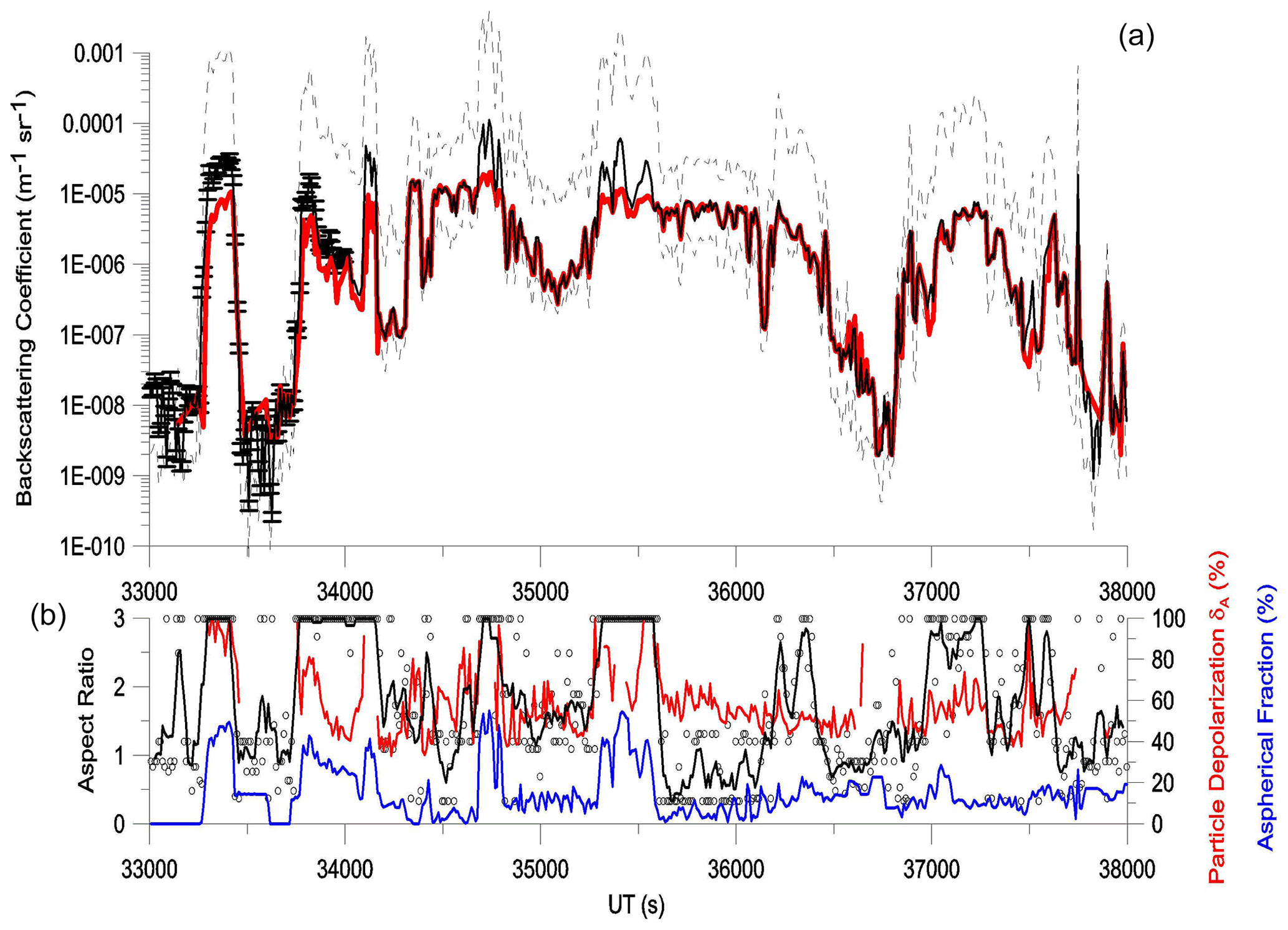
Figure 3(a) Red line: time series of particle backscattering coefficient β measured by MAS on 10 August 2017; solid black line: best optical-modeling match βNC – error bars are displayed in the first part of the curve; dashed black lines: maximum and minimum values of the optical-modeling values. (b) Red line: particle depolarization measured by MAS; blue line: particle aspherical fraction measured by NIXE-CAPS; black dots: AF values of the best optical-modeling match βNC; black line: a five-point running average.
As a test for the arbitrariness of the choice of AR that ensures the best agreement with the measurements, we looked for possible correlations between the selected AR and (i) the particle depolarization δA and (ii) the fraction of aspheric particles (AF). In the lower panels of Fig. 3, the AR that provided the best match is reported (black line) together with the observed particle depolarization (red line) and the particle AF as measured by NIXE-CAPS (blue line). We note that the AR values that made the best match are arranged according to a certain temporal continuity, and we can identify well-defined time intervals in which their values remain almost constant. This is encouraging to think that the choice of AR that best matches the measurements is not exclusively an exercise of handpicking but rather reflects characteristics of the average morphology of the measured particles. It is of particular interest to note that regions with AR =3 – which provides the lowest – almost always coincide with regions in which the NIXE-CAPS has observed the highest particle AF. This, in turn, is often correlated with high values of total depolarization. Moreover, looking at the entire dataset, we have noted a tendency to have ARs close to 1 associated with small β values and depolarization of less than 20 %, while ARs greater than 1.5 and less than 0.5 favor medium–high β values and depolarization greater than 20 % (see Fig. A7 in Appendix A).
We have explored a possible lack of linearity in the response of the backscattersonde at high backscattered signals as a possible cause of the discrepancy between the highest calculated and measured β. The linear response of the backscattersonde was checked in the laboratory before the campaign deployment. This was done by screening the receiving optics with a series of calibrated gray filters and controlling the response of the instrument to pulsed light of various intensities. This procedure was repeated at various levels of background light. For the present study, a further test was carried out by comparing the backscattering coefficient observed during the campaign by the backscattersonde in some of the thickest clouds on 8 August 2017 between 05:17 and 05:50 UTC (19 000 and 21 000 s; see Fig. A8 in Appendix A) and on 10 August 2017 between 10:00 and 10:33 UTC (36 000 to and 38 000 s) with that observed by the two MAL lidars on board the Geophysica. These two lidars point, respectively, upwards and downwards, providing profiles of backscatter ratio and depolarization. We have used signals from the closest lidar range, in its partial overlap region, and processed them as if they came from backscattersondes. The average of the two lidar backscattering coefficients observed by them at a distance of 500 m upwards and downwards was then compared with that observed by MAS. The data have been averaged over 60 s. The result is displayed in Fig. 4. Despite the scattering of the data points, which might be attributed to a lack of vertical homogeneity of the cloud, it shows that there is a good correlation between the backscattering coefficient measured in situ and that measured at close range. The lidar backscatter signal is measured in photon-counting mode. The linear dynamic range is identified to be below the count rate of approx. 1.5 MHz. The complete signal saturation is noticed to be a count rate of approx. 15 MHz. For the cases reported here, the signals are at the level of some tens of KHz, i.e., well inside the linearity range. Thus, we may exclude any loss of linearity. As a result, we are tempted to exclude a severe loss of linearity of the backscattersonde and a consequent significant underestimation of the largest backscattering coefficients observed by it. Further sustaining our conclusion, we note that the overestimation of the optical model also appears in regions where saturation of the backscattersonde signal should not be expected, for instance, around 34 000 s on the 10 August 2017 flight.
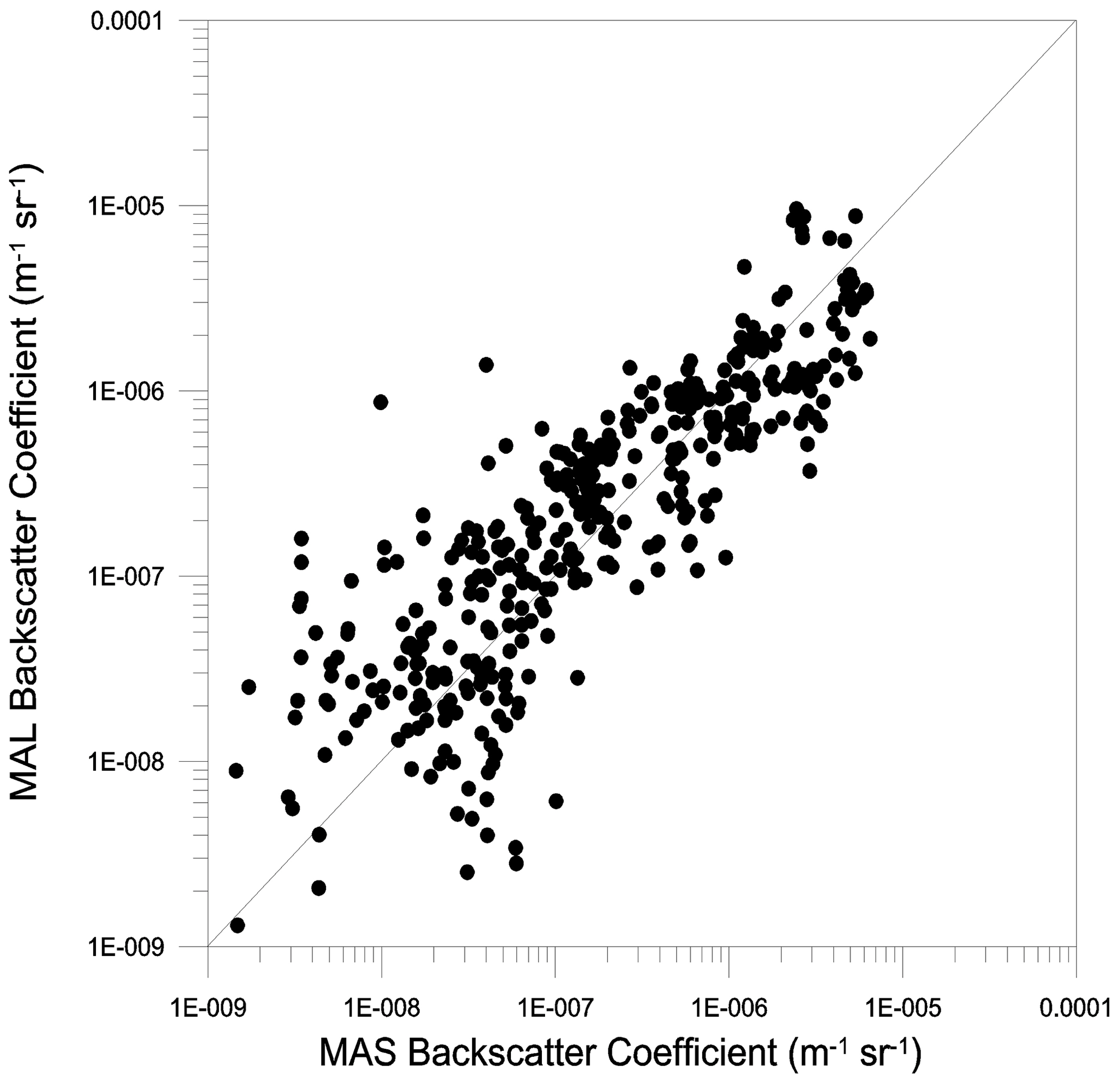
Figure 4A 2D histogram of particle backscatter coefficient observations from the backscattersonde MAS and the particle backscattering coefficient data from the two MALs, pointing upwards and downwards, at 500 m from the aircraft. The average of the two lidar backscattering coefficients has been used for the comparison. The data have been averaged over 60 s. In the graph are the 500 data points acquired while crossing some of the thickest clouds observed during the campaign.
Figures 5 and 6 report the two-dimensional histograms of occurrence of the measured–calculated backscattering coefficients and particle depolarization. While for the β the agreement is good and the analysis of the whole campaign dataset confirms what has already been shown in the previously discussed time series, i.e., an underestimation of the βNC for values of β below m−1 sr−1 and a slight overestimation for high values in a relatively insignificant number of cases, the agreement for the depolarization is not good. From the inspection of Fig. 6 we see that there are few cases when the two depolarization lines up to a 1 : 1 correlation. However, for a considerable number of observations, the calculated depolarization remains around 10 %, while the measured one varies throughout its range of variability. Moreover, the optical-modeling performance is very poor in reproducing the measured depolarization. We have tested how to improve the agreement by linking the choice of AR to match with depolarization rather than with backscattering. Of course, the comparison between measured and modeled depolarization improves but in the same way leads to a larger disagreement in the backscatter, which in many cases is strongly overestimated by the optical model by up to 1–2 orders of magnitude (see Fig. A9 in Appendix A). Even where the agreement between the calculated and the measured β is kept within 1 order of magnitude, it fails to reproduce effectively the experimental dataset, as reported in Figs. 5 and 6. In some ways it is unfortunate not to be able to simulate backscattering and depolarization simultaneously with a single choice of AR. However, we are aware of the fact that the modeling of depolarization is an open and highly challenging problem, one that is not easy and that is perhaps impossible to solve given the wide variety of shapes that atmospheric ice crystals can take (Liou and Yang, 2016). For this reason, we prefer to keep our comparison between optical measurements and calculations limited to the backscattering coefficient.
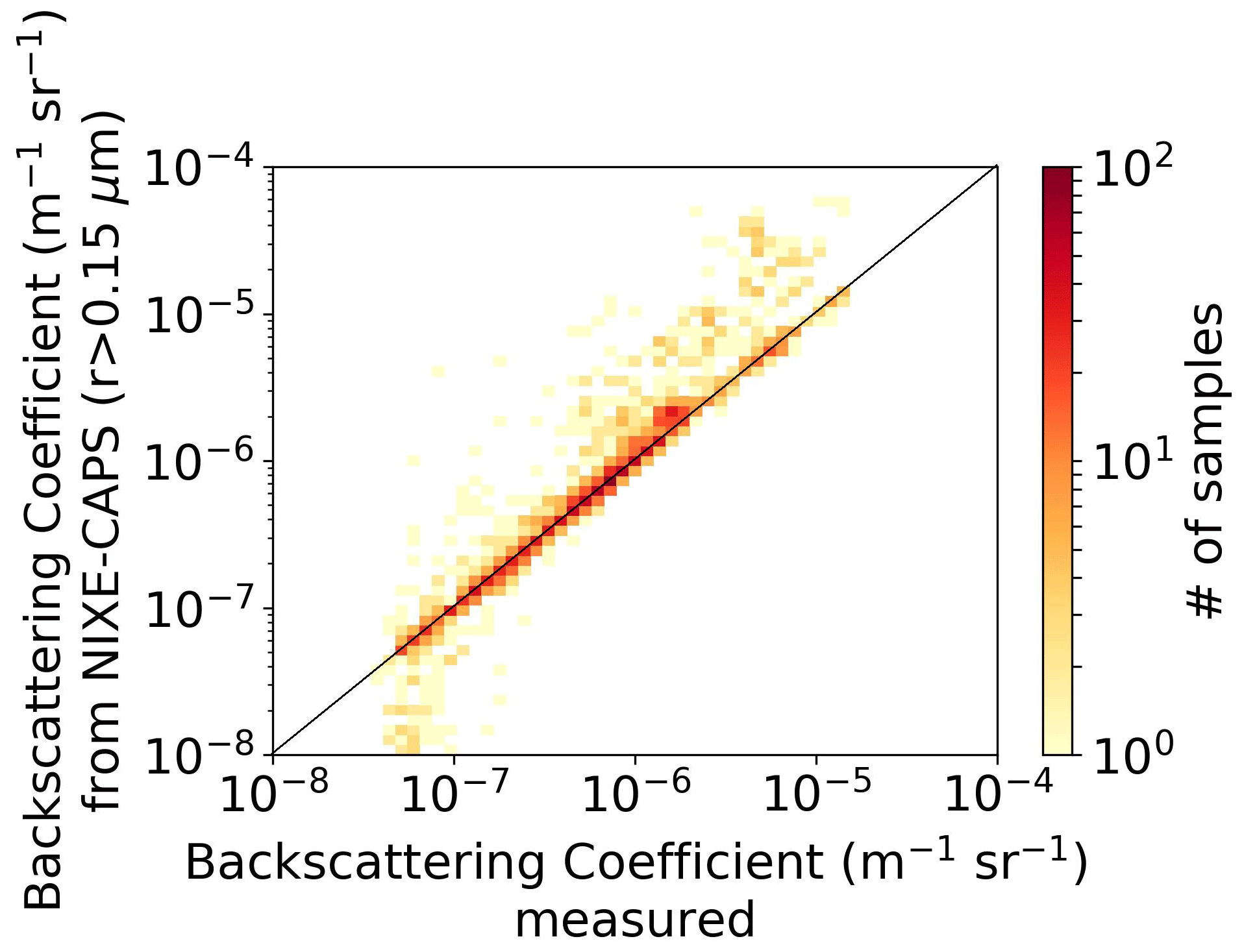
Figure 52D histograms of occurrence of the measured and calculated backscattering coefficients. Data were acquired throughout the campaign by the MAS backscattersonde. The color codes the number of observations in the 2D bin.
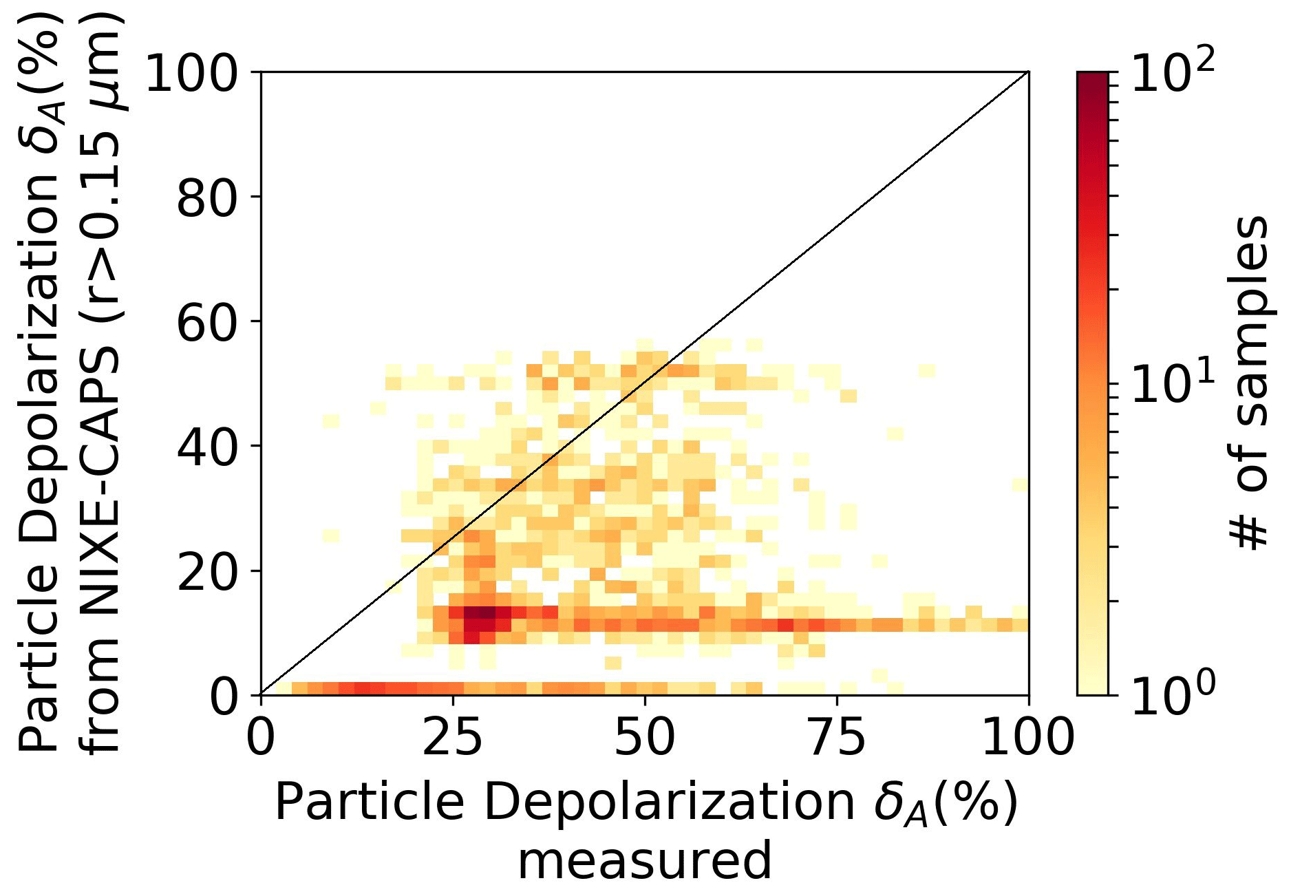
Figure 62D histograms of occurrence of the measured and calculated particle depolarization. Data were acquired throughout the campaign by the MAS backscattersonde. The color codes the number of observations in the 2D bin.
4.3 Backscattering versus particle size distribution bulk parameters
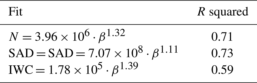
Figures 7, 8, 9, 10, and 11 show Nice, Rmean, Reff, SAD, and IWC as functions of β, respectively. In the graphs, the black lines represent regression curves, parameterized in the general form . The coefficients of the regression are reported in Table 1 together with the R squared of the fit. The dataset has been fitted between the limits and m−1 sr−1, which have been chosen to maximize the goodness of the fit and to try to avoid outliers at the extremes of the variability range. We can regard those regression curves as guides for estimating the microphysics bulk parameters of the clouds and their variability range from remote measurements of cloud optical parameters.
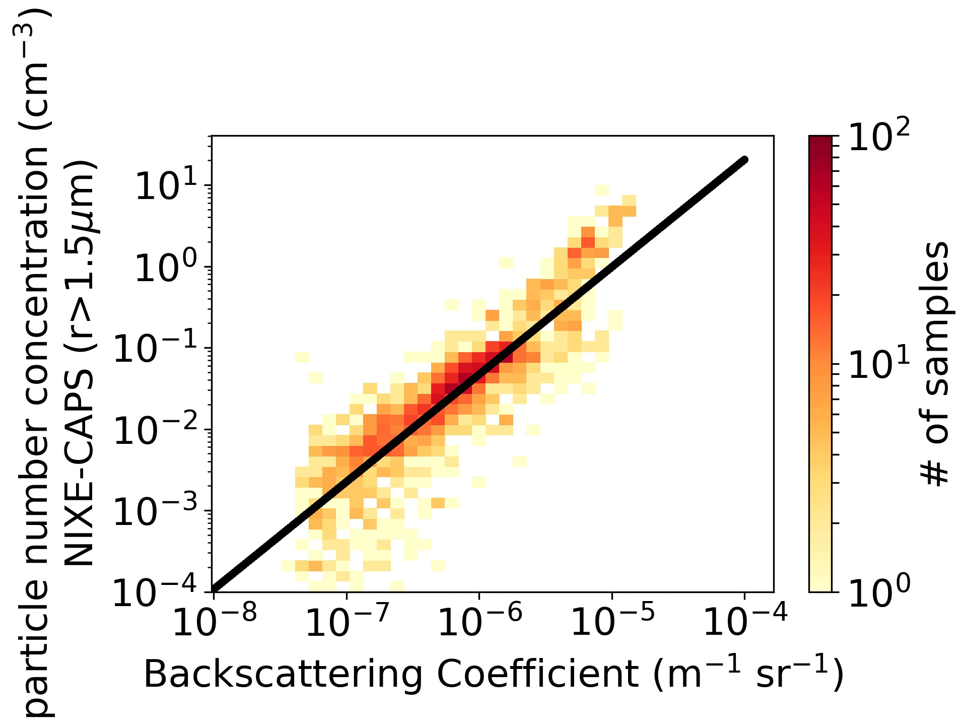
Figure 7A 2D histogram of particle backscattering coefficient observations β from the backscattersonde MAS and particle number concentration N. The black lines represent the fit . Data were acquired throughout the campaign by the MAS backscattersonde. The color codes represent the number of observations in the 2D bin.
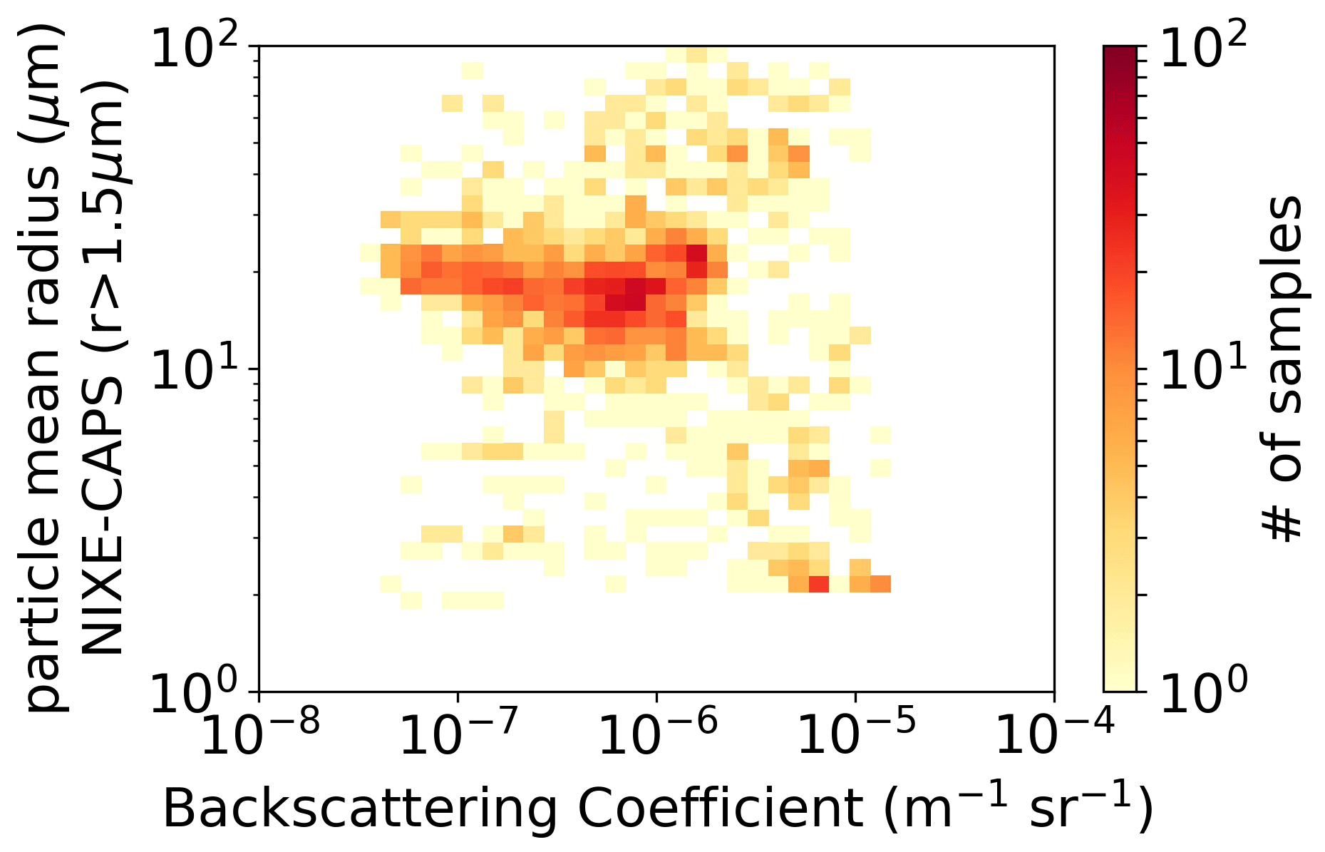
Figure 8A 2D histogram of particle backscattering coefficient observations β from the backscattersonde MAS and particle mean radius Rmean. Data were acquired throughout the campaign by the MAS backscattersonde. The color codes represent the number of observations in the 2D bin.
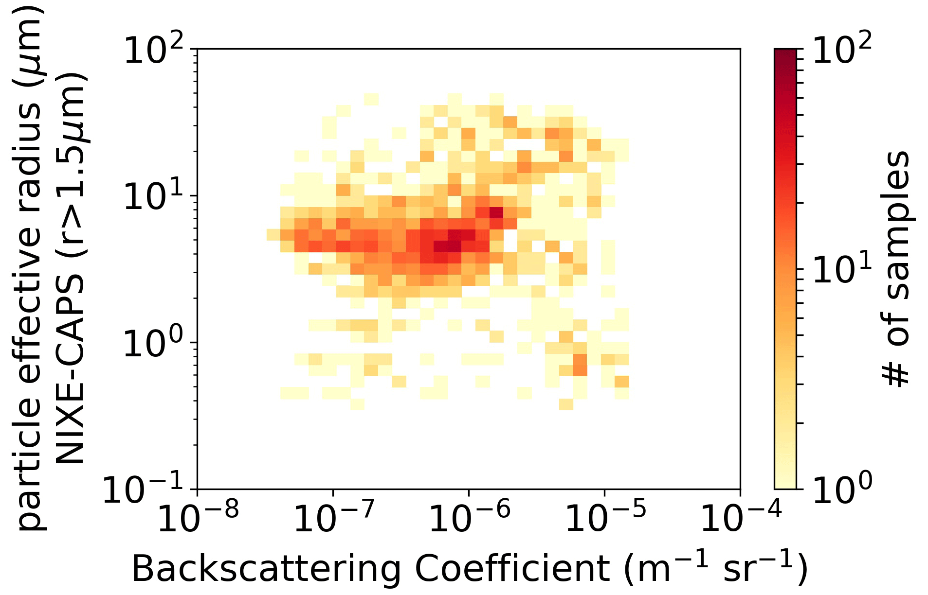
Figure 9A 2D histogram of particle backscattering coefficient observations β from the backscattersonde MAS and particle effective radius Reff. Data were acquired throughout the campaign by the MAS backscattersonde. The color codes represent the number of observations in the 2D bin.
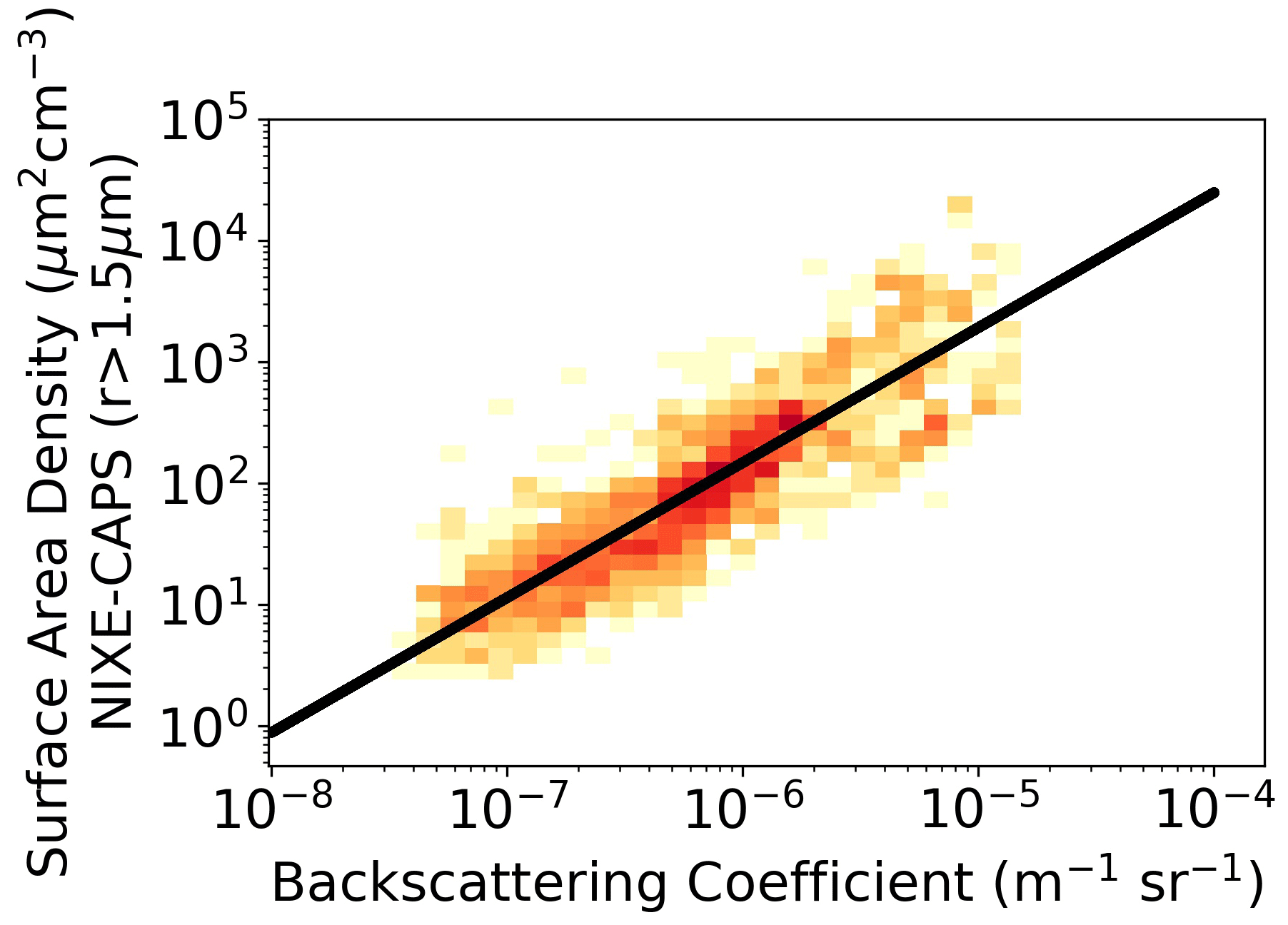
Figure 10A 2D histogram of particle backscattering coefficient observations β from the backscattersonde MAS and particle surface area density (SAD). The black line represents the fit SAD . The color codes represent the number of observations in the 2D bin.
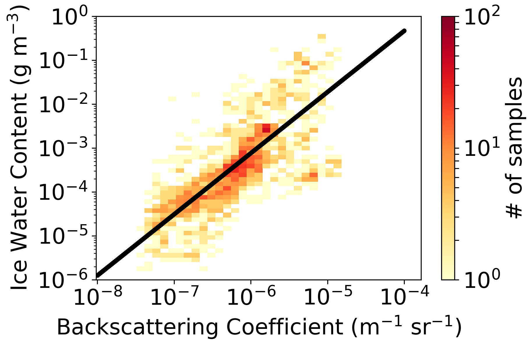
Figure 11A 2D histogram of particle backscattering coefficient observations from the backscattersonde MAS and ice water content (IWC). The black line represents the fit IWC . The color codes represent the number of observations in the 2D bin.
Table 1Parameterizations linking the backscattering coefficient to particle number, surface area density (SAD), and ice water content (IWC). Here β is expressed in meters per steradian (m−1 sr−1) while N, SAD, and IWC are expressed respectively in cubic centimeters (cm−3), square micrometers per cubic centimeter (µm2 cm−3), and grams per cubic meter (g m−3).
The linearity between β and Nice (Fig. 7) is quite striking and indicates that β basically scales with the cloud particle number density Nice, as well as SAD and IWC. Hence, this suggests that the various shapes of the PSD in our observations hardly change the scattering properties of the clouds. This finding is further confirmed by the linearity seen between β and SAD or IWC (Figs. 10, 11) and the lack of clear correlation between β and Rmean or Reff (Figs. 8, 9).
With simple analytical calculations on various types of functional forms for the PSD (gamma, lognormal, etc.) and in the spherical ice approximation, it is easy to demonstrate that a dependence on the square of the modal radius – and hence on other similar parameters linked to it, such as the mean or the effective radius – and on the total number of particles is indeed to be expected for β, i.e., , as the physical intuition would also suggest. In our case, such a dependency on Rmean, which varies by a factor of 2, is masked by the much wider variability of N0, which varies by over 5 orders of magnitude.
4.4 Depolarization, aspherical fraction, and PSD parameters
4.4.1 Depolarization vs. aspherical fraction
In our study, we have looked for and found no direct correlation between particle depolarization observed with the backscattersonde and PSD aspherical fraction (AF). AF has peaks around 60 % but on average is maintained around values of 20 %, while the corresponding values of the depolarization span its entire range of variability, giving an unclear relationship between the two quantities (see Fig. A10 in Appendix A). Figure 13 clearly shows again the positive correlation between BR and Nice. This relationship is independent from the polarization δTA throughout the BR range, except at the highest BR values. There, we note how, for the same extreme values of BR, low δTA values are associated with low Nice, high δTA, and high Nice.
This is possibly because the maximum detectable AF of ice particles decreases with the size of the particles. The reason is that the depolarization signal becomes weaker with decreasing ice particle size and also that the ice particles become less and less aspheric, and the backscattersonde and the cloud spectrometer have depolarization sensitivities that vary differently with the size of the scattering particle.
In order to display other parameters along with the former two, which may help us find and possibly disentangle a link between these two quantities, we choose to represent our dataset in a δT–BR space (in fact, for ease of scale, is used instead of BR) and to color code the points with AF, N, Rmean, and temperature T as possible parameters of interest.
We remind ourselves here that δT is not as an intensive quantity as δTA since it simultaneously depends on the average shape of the cloud particles, but also on the backscattering of the whole particle distribution, i.e. on the particle number concentration, or SAD. Hence, for a given and fixed particle shape and dimension, δT increases with the BR to a limiting value, which is δTA. It is the latter true intensive quantity that depends solely on the particle's average morphology. In fact, Adachi et al. (2001) demonstrated that, in a plot of δT towards , the experimental points of clouds composed of particles sharing the same shape and size but with variable particle number density (i.e., variable BR) will arrange themselves along a straight line, starting at δmol for BR =1 (this is the case when no particles are present, i.e., when δT attains its molecular value δmol (Young, 1980)) and ending at a δTA for BR =∞ with this δTA depending on the particular shape and size common to all particles. So, in this (BR, δT) graph, ice clouds composed of particles with the same δTA and different BR (which we may take as a proxy for particle number concentration) would be distributed along a line starting at δmol for BR =1 and trending towards a particular δTA when extrapolated to BR =∞. The value of such δTA depends on the average morphology of the cloud particles. Therefore, we may imagine the data point distribution as being composed of linear series of points starting at δmol and spanning the triangle: each line of data points represents the results of the measured variable particle number concentration at constant depolarization properties of the particles as encountered in the clouds. Conversely, if we were to report data points from clouds composed of particles with different shapes and sizes, these points would be distributed within a triangle whose vertices are δmol for BR =1 and δTA max and δTA min for BR =∞. It should be noted that, if among the possible particle shapes the spherical one is included, then δTA min would attain a 0 value.
In Fig. 12 we report our dataset, with the data points from in-cloud measurements (i.e., BR >1.2, ) color coded in terms of AF. The y-axis intercepts at BR =∞ give us the range of variability of δTA, which, for our cirrus, ranges approximately from 20 % to 50 %. Inspecting the figure, we may argue that clouds with medium AF are often linked to intermediate values of δTA over the whole BR variability range, while clouds with high AF, associated with high BR, show no clear correlation with δTA. Interestingly, clouds with low AF show up at both low BR (with low to intermediate depolarization) and high BR (with intermediate to high depolarization). The conditions at the highest BRs are in fact noteworthy: there, we have both the highest values of the AF for δTA min and δTA max and the lowest values of the AF in a range spanning from δTA med to δTA max.
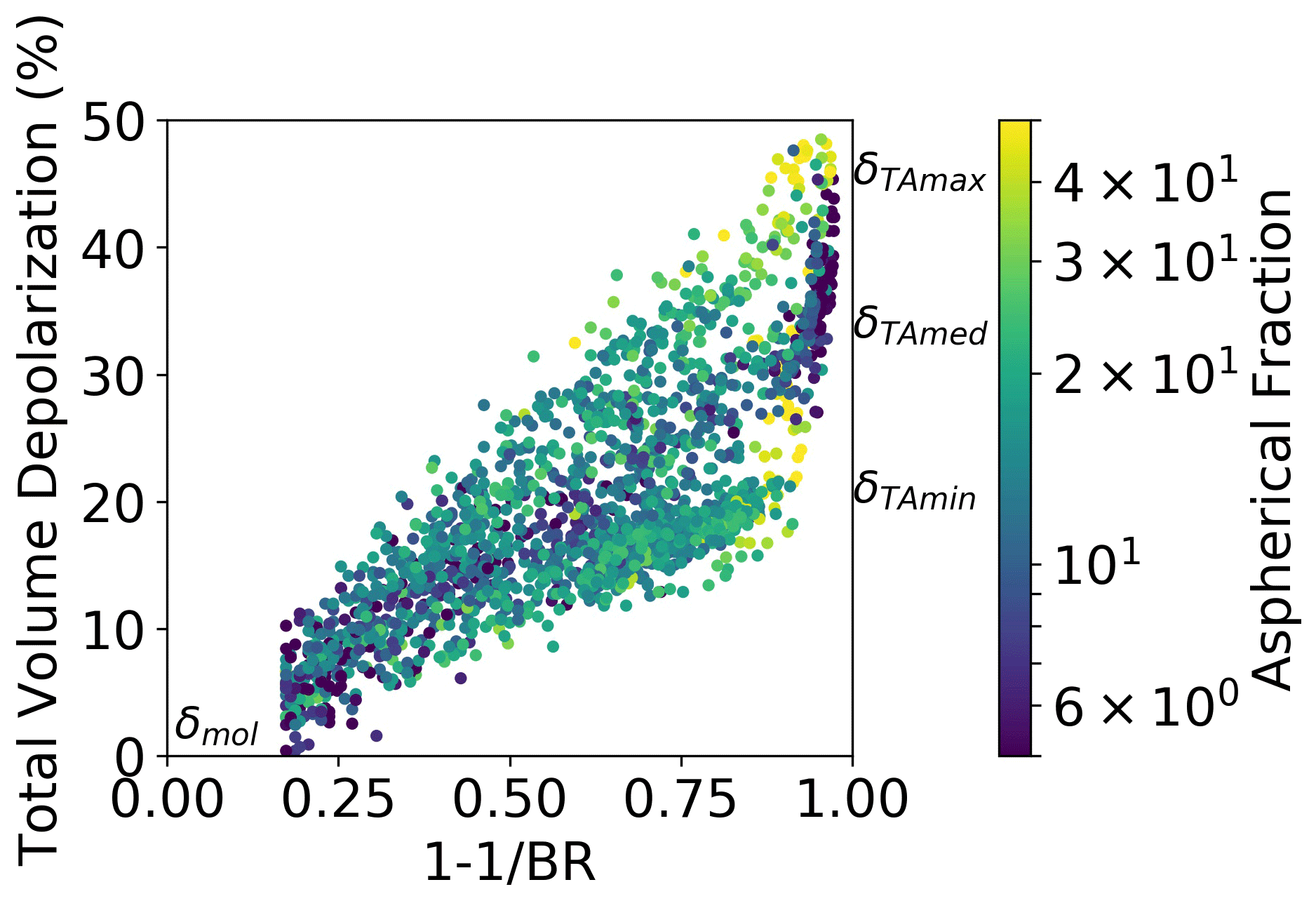
These relationships between BR, depolarization, and AF probably reflect aspects of the morphology, size, and numerical concentration of the cloud particulate, but they are not straightforward to interpret unambiguously. To seek a better understanding, we present in similar plots the dependence of depolarization on Nice and Rmean and on temperature.
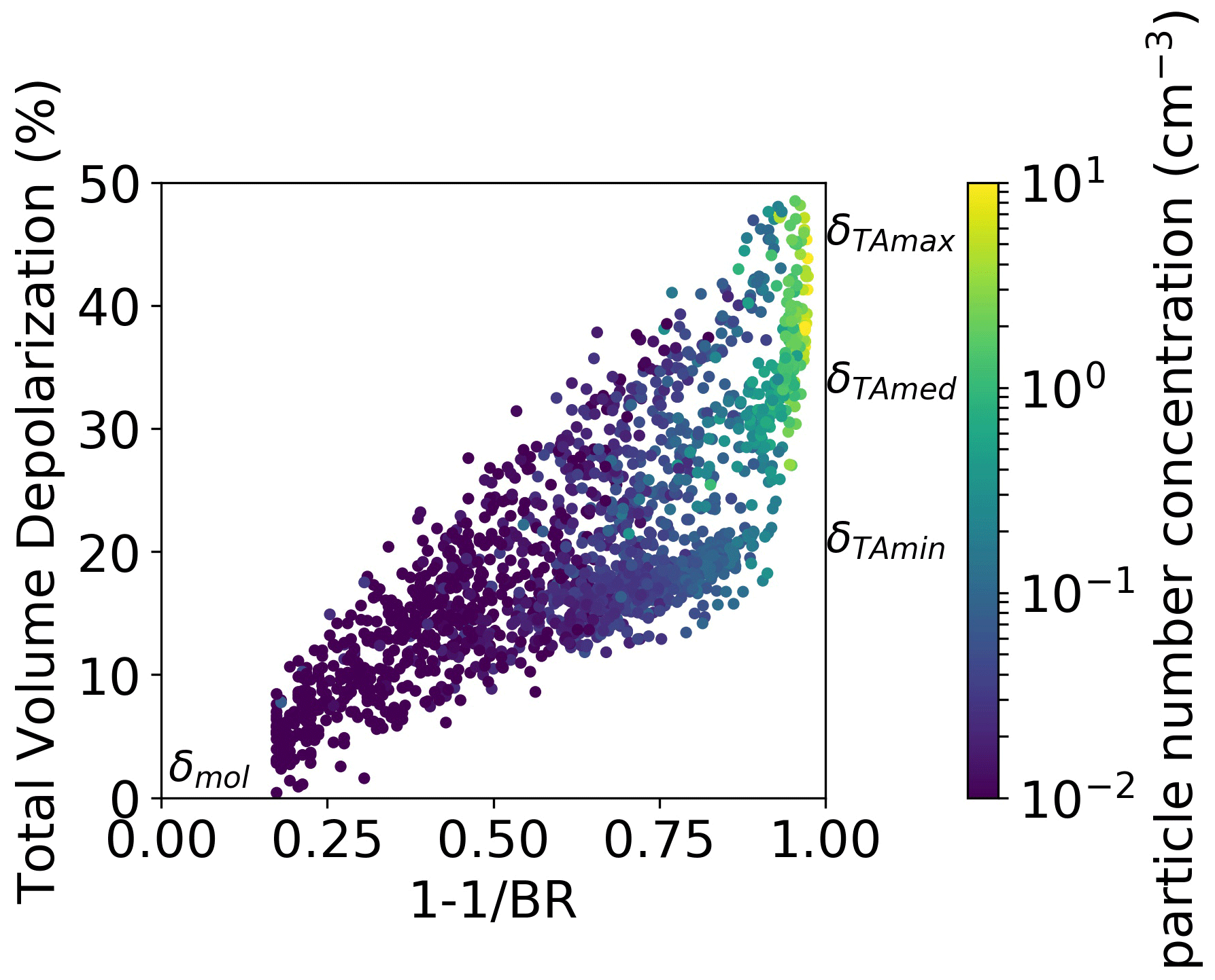
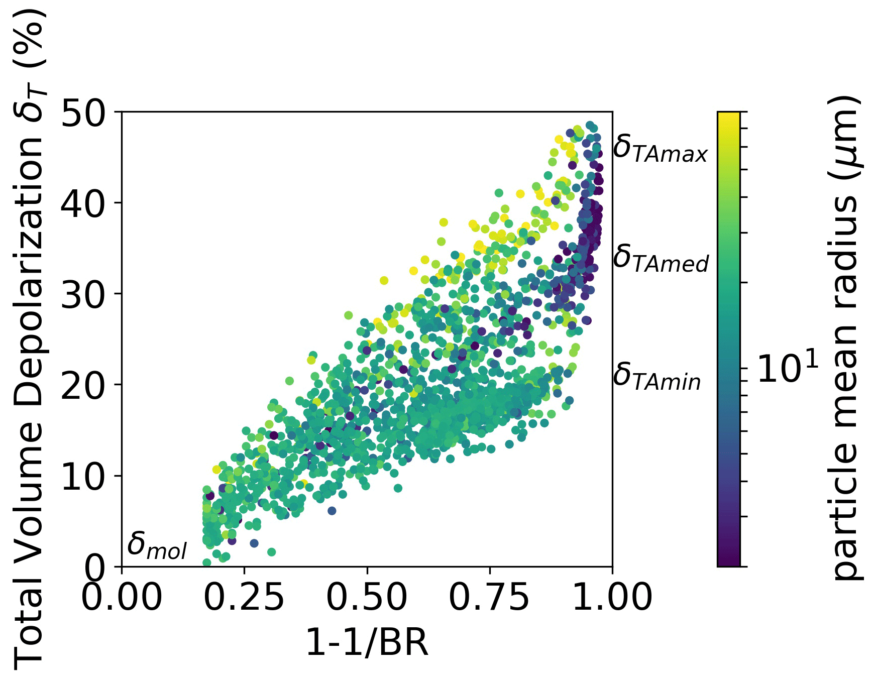
4.4.2 Depolarization vs. particle number concentration, mean radius, and temperature
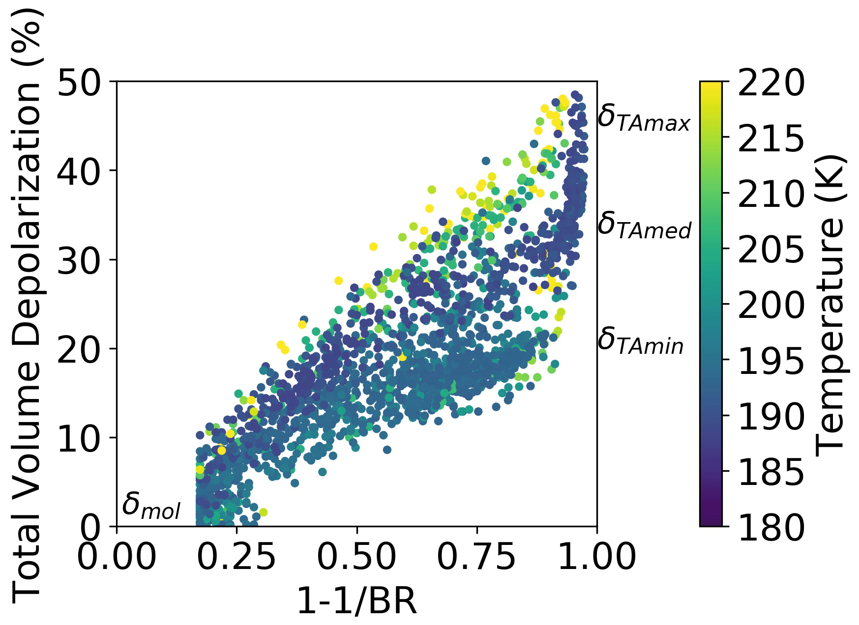
We show in Fig. 13, using the same δT–BR framework, the data points color coded in terms of Nice, and in Fig. 14 we show the same data points color coded in terms of Rmean. Figure 13 clearly shows again the positive correlation between BR and Nice independently of the polarization of δTA, except at the highest values of BR, where there appears a positive correlation between δTA and Nice. Figure 14 shows how high δTA values are often associated with high Rmean (red dots along the line δmol–δTA max), and again, peculiarly in the same region of the highest values of BR, small Rmean coincides with medium to high δTA. In Fig. 15, we show the same dataset, this time color coded in terms of temperature. The points at temperatures above 200 K show both very high and, although in smaller numbers, very low depolarization with intermediate to high BR values. Points below 200 K show the general tendency towards an increase in depolarization at colder temperatures, which was already commented on in Fig. 2. It is noteworthy that the observations in the region of very high BR and between δTA med and δTA max, where the coldest temperatures, large particle concentration, low AF, and low mean radius have been met, are worthy of a special mention. These all came from clouds encountered in a single flight, performed on 10 August 2017. On that flight, a convective overshooting updraft of probable liquid origin, with very large aggregates and a significant number of freshly nucleated cloud particles, was met together with a younger outflow of the overshoot with both growing small particles and sedimenting large ones (Krämer et al., 2020 – see their Fig. 10b; Khaykin et al., 2022). This dynamic and therefore particularly variable situation makes the overall interpretation of the observed parameters exceptionally complicated.
As stated at the beginning of the paragraph, there seems to be no direct correlation between δTA and AF, and although some clustering of the variables is possible, these clusters often overlap. It is possible that additional information on particle shape, which is missing in the present study (a measured aspect ratio would be an obvious candidate), would help disentangle the variables.
As outlined in the previous paragraph, in our study, the T matrix has been used directly to model the scattering properties of particles up to a few hundred size parameters and indirectly to estimate the depolarization and the modification of Mie backscattering for larger particles. We note that, while Mie theory strictly applies to spherical particles, it has no upper size limit and can be applied to the entire cloud particle size range.
Despite the limitations outlined above, some conclusions can be deduced from our study. It is possible to make the measurements coincide with the optical modeling through a suitable and reasonable choice of the particle AR, and this reassures us about the compatibility of the two datasets. This choice generally favors high ARs (i.e., high Mie backscattering depression) in regions of high backscattering and high depolarization and with a large presence of AF, while ARs near to or less than unity are chosen when backscattering is medium to low and when the presence of AF is not very pronounced. In general, the choice of AR produces a high depression of the backscattering compared to Mie's predictions, and this depression increases with increasing presence of aspherical scatterers to exceed 1 order of magnitude when AF is large. In cases with particularly high backscattering, our optical model produces backscattering higher than those observed. If – as seems to be appropriate – non-linearity problems in the backscatter probe are excluded, it is quite possible that, to reduce the computed backscattering and reconcile it with observations, we would need to use ARs beyond the limits considered in our optical model.
Moreover, it is clear from our simulations that the greatest ambiguity in the results of the observed versus the calculated comparison is linked to the choice of the particles' morphology rather than to uncertainties in the determination of the PSD or in the measurement of backscattering.
Another interesting result is the identification of the size range of the particulate matter that most contributes to the observed backscattering. For all the PSD under study, we have examined the cumulative function (Eq. 18)
of the respective β as a function of the particle radius in order to determine the buildup of the final values of the particle backscattering coefficient in relation to the particle radius. We have used Mie codes to give an upper limit to such computation. The histogram of the values of the cumulative distributions as a function of the particle radius is shown in Fig. 16. It can be seen from the analysis of the histogram of cumulatives that the values of the backscattering coefficient are formed mainly in the dimensional range below 300 µm and that particles with radii greater than 400 µm do not significantly contribute to the β. This analysis gives us confidence in affirming that the size range of the detected particles is sufficient to fully characterize the backscattering coefficient.
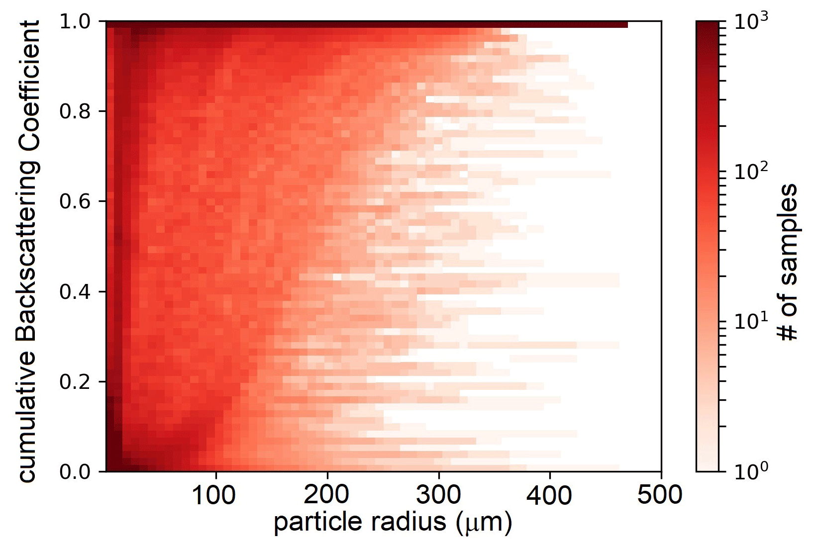
Figure 16A 2D histogram of cumulative distributions of particle backscattering coefficient computation. The histogram shows the buildup of the particle backscattering coefficient with respect to the particle radius for all the PSDs under study. For the present graph, Mie scattering computation has been used.
The T-matrix computation of depolarization gives no satisfactory results, being that the modeled depolarization is underestimated in comparison to the depolarization measured by MAS. It is possible that this is due to the specificity of our approach. Our computations are not able to produce δA higher than 40 % in the large-particle regime (i.e., radius grater than 10 µm). Other theoretical depolarization ratios computed from a unified theory of light scattering by ice crystals for shapes including bullet rosettes, solid and hollow columns, Koch snowflakes, and plates, extend up to 60 % and more (Liu and Mishchenko, 2001). As stated previously, there seems to be no clear correlation between particle depolarization and AF. Particle depolarization increases with temperature and with Nice at high backscattering. High depolarization is often, but not always, associated with high Rmean as there are cases where, at high values of backscattering, small Rmean coincides with medium to high δTA. This study therefore suggests that, although some correlations can be discerned between the depolarization and the environmental conditions in which the cloud is observed or its microphysical and morphological average parameters, there are a lot of exceptions. These probably depend on the history of the formation and the instant of the evolution of the cloud, leading to the coexistence of cloud particles with different morphologies and sizes. Hence, the study does not allow us to formulate general rules that link depolarization to the microphysics of the cloud.
The regression of the backscattering coefficient with respect to the various bulk parameters of the cirrus clouds (Nice, Rmean, Reff, SAD, and IWC) is therefore based on a solid foundation. Effectively, similar regressions were presented in Cairo et al. (2011) based on cirrus particle measurements from an FSSP-100. There, the upper detection limit of the instrument was 15.5 µm in radius, while in the present study, this limit has been extended upwards by more than 1 order of magnitude. So, although the present figures are qualitatively similar to those of Cairo et al. (2011), some difference is to be expected due to the larger range of particle radii that is now covered. The limitedness of the radius range was a caveat already advocated for in the aforementioned work. In fact, the larger detection threshold impacts all the regressions, which results in an underestimation in Cairo et al. (2011) of Nice, SAD, and VD. In the present work, the detection of a wider particle dimensional range, including the radii which determine most of the measured backscatter coefficient, allows us to place more reliability on the regressions here presented.
The relative independence of β from Rmean and Reff confirms that Nice is the main parameter governing the cirrus scattering properties at optical wavelengths. This finding would imply that the shapes of the PSD should not play a major role and should all share a similar shape once normalized for the total number of particles, at least for low to medium β values. For high β values, the spreading of the corresponding PSD gets larger, suggesting that such observations originated from clouds with both very large and few particles and small and more numerous particles. Konoshonkin et al. (2017b) computed the backscattering Mueller matrix for the typical shapes of ice crystals of cirrus (hexagonal columns and plates, bullets, and droxtals) in the case of their random orientations and for crystal sizes from 10 to 1000 µm with a physical-optics approximation code and proposed using the backscatter-to-IWC ratio (as well as the extinction-to backscatter ratio – LR) for inferring the crystal size in the clouds. Figure 17 shows such a ratio versus Rmean, which, in fact, shows such a linear relationship for Rmean values larger than 10 µm, while for lower values, a different linear behavior might be discerned. In Fig. 17, the black line is a regression of the form , which has been estimated for Rmean from 10 to 100 µm. The R-squared value of the fit is 0.54, which does not allow us to conclude that such a relationship is possible based on solid foundations. Because of this, such a regression should be used with great caution to estimate Rmean when β and IWC are independently available.
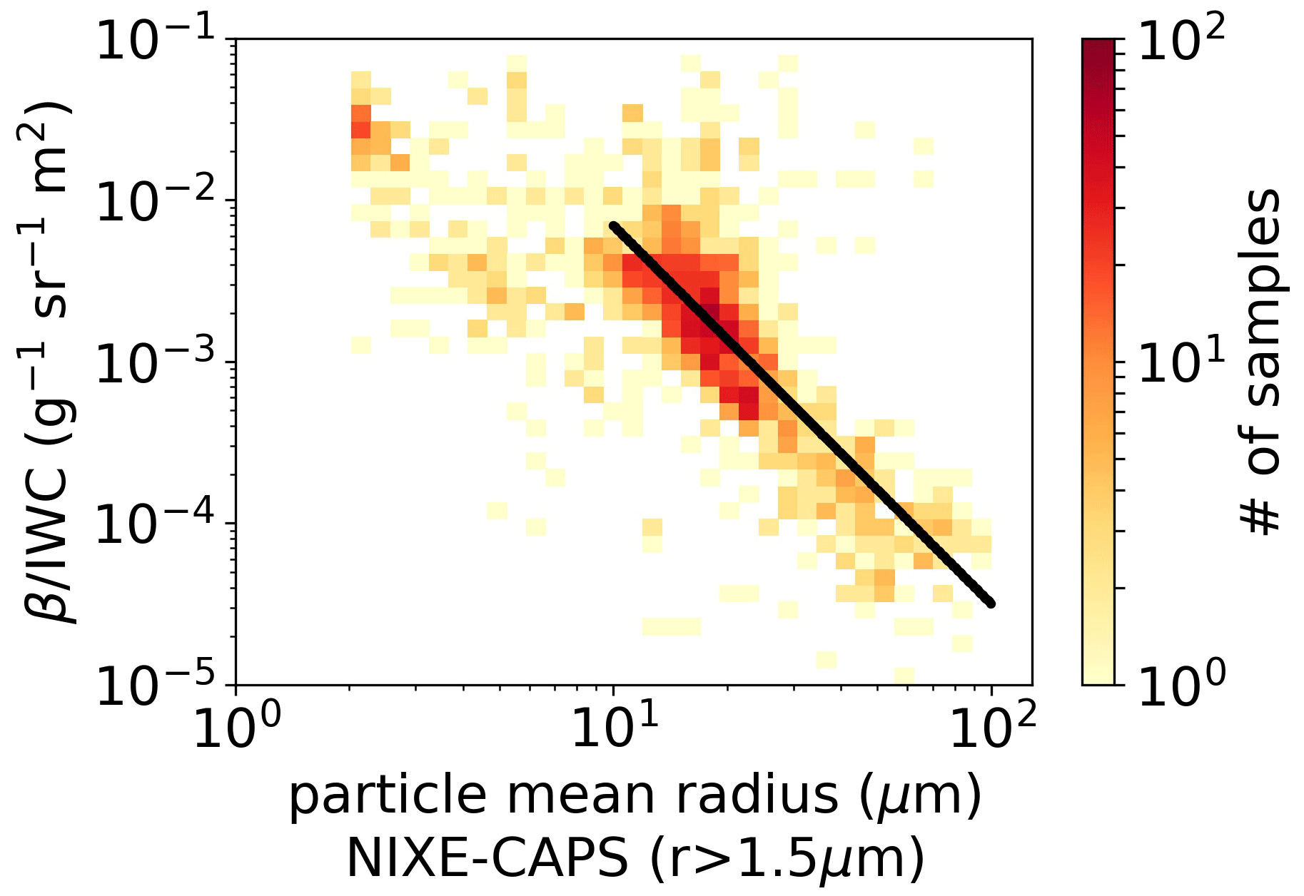
Figure 17A 2D histogram of the ratio of the backscattering coefficient in relation to IWC versus particle mean radius. The black line shows a regression computed for Rmean from 10 to 100 µm. The fit is , with an R-squared value of 0.54. The color codes represent the number of observations in the 2D bin.
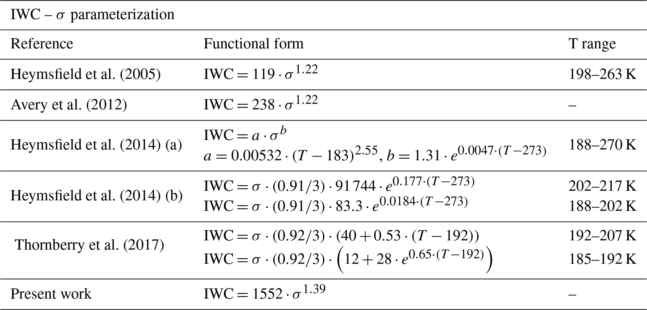
Several studies have provided an estimate of the dependence of the IWC on lidar extinction (Heymsfield et al., 2005; Avery et al., 2012; Heymsfield et al., 2014; Thornberry et al., 2017). They are based on in situ measurements of IWC and PSD, with the latter being used to provide an estimate of the lidar extinction from optical modeling of the cloud particles. These IWC–σ relationships could be compared with our IWC estimates based on β if a suitable extinction-to-backscatter ratio (i.e., lidar ratio – LR) is chosen. Unfortunately, LR can vary from 10 to 40 sr in tropical cirrus clouds (Chen et al., 2002), thus making the comparison somewhat arbitrary. Using LR =30 sr as the most probable value (Balmes et al., 2019) and using , we can correlate our IWC measurements with σ. Figure 18 is thus the analogue of Fig. 11, where this time IWC is re-parameterized as a function of σ. The same figure shows the analytical relationship obtained in this work (solid black line) along with those present in the literature, shown in Table 2. Although all parameterizations capture the IWC–σ trend and align with each other in the lower range of data variability, the result of our study is in agreement with only Avery et al. (2012), while it diverges from the other parameterizations, more severely for those that depend on the temperature. This especially the case in the upper range of data variability. It should be noted that, in this range, the data themselves also have a greater dispersion. We want to underline the limits of this comparison: in the case of the present study, they are caused by having chosen, rather arbitrarily, the same LR value for all the clouds observed, and in the case of the other parameterizations, they are caused by having used an indirect determination of the extinction, calculated from the PSDs. It would be very interesting to have simultaneous in situ observations of backscattering, extinction, and IWC available in the future.
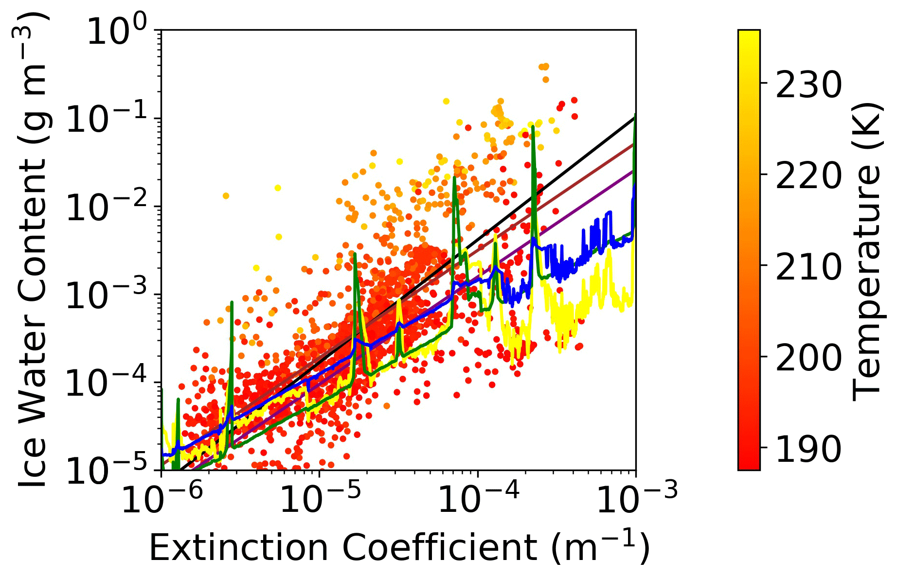
Figure 18Scatterplot of measured IWC vs. estimated extinction σ=30β. The solid lines represent regressions from (i) the present work, black; (ii) Heymsfield et al. (2005), purple; (iii) Avery et al. (2012), brown; Heymsfield et al. (2014), yellow and green; Thornberry et al. (2017), blue. Experimental points are color coded in terms of the temperature of the observation.
Table 2IWC–σ parameterizations (adapted from Thornberry et al., 2017). IWC is expressed in grams per cubic meter (g m−3), and σ is expressed in meters (m−1). In Heymsfield et al. (2014), (a) is retrieved from direct measurements of IWC; (b) from IWC estimated from PSD.
To conclude, we provide a comment on the representativeness of our study. The range of backscattering values observed during campaign activities is wide and covers the variability of possible lidar observations from satellites (Balmes et al., 2019). Regarding the type of cirrus clouds observed, during the campaign activities, both in situ and liquid-origin clouds were sampled, but the second type was dominant since most of the observations came from penetration into the outflow regions of deep convective clouds. As there might be differences in the microphysical properties of the cirrus depending on the formation process (Lawson et al., 2019; Krämer et al., 2020), especially in the initial stage of their life cycle, the results presented here are not necessarily representative of all cirrus that can be observed from space.
Measurements in cirrus clouds obtained during the StratoClim campaign by two dual-instrument cloud spectrometers, two hygrometers, and a backscattersonde have been compared. The comparison of the microphysical data with the optical observations of the backscattersonde was performed by calculating the cirrus particle backscattering coefficient from the PSD by means of optical modeling. A proper adjustment of the modeled particle AR allows us to match the optical computation with the backscattering observations. Relations have been obtained to link the ice particles' backscatter coefficients to their concentrations, their means and effective radii, surface area density, and ice water content. These results confirm and expand upon similar studies and allow us to estimate, within 1 order of magnitude, data of bulk cirrus microphysics from lidar remote sensing observations.
The comparison between particle depolarization from the backscattersonde and the aspherical fraction measured by one of the cloud spectrometers shows no univocal relationship between the two quantities, and we ask therefore for further investigations where additional information on particle morphology may be required.
We include in this appendix, in Figs. A1 and A2, the particle backscattering coefficient and depolarization vs. the particle radius, parameterized with the particle AR. These optical parameters have been computed for a reference monodisperse PSD with a particle concentration of 1 cm−3. In Fig. A3, we show the comparison of the backscattering coefficient computed with SDs with lower size limits at 0.3 (y axis) and 1.5 (x axis) µm. Mie codes have been used in the computation. In Figs. A4 and A5, we show the 2D histogram of the particle concentration Nice and particle mean radius Rmean computed from PSD from NIXE-CAPS (x axis) and CCP (y axis). Figure A6 shows the particle backscattering coefficient computation from NIXE-CAPS (x axis) and CCP (y axis), with Mie scattering codes. Figure A7 shows the scatterplot of the total particle depolarization vs. the aspect ratio, color coded in terms of the backscatter coefficient. In Fig. A9, we show the results of the backscattering comparison in the case when the AR was chosen to make the depolarization match. In the figure, the time series of the particle backscattering coefficient β measured by MAS on 10 August 2017 (red lines) is shown (solid black line), with βNC corresponding to the best match between measured δ and computed (the latter in not displayed); error bars are reported in the first part of the curve, and the dashed black lines represent the maximum and minimum values of the optical-modeling values. In the lower panel, the red line represents the particle depolarization measured by MAS, the blue line represents the particle aspherical faction measured by NIXE-CAPS, and the black line represents the AF values of the best match between measured δ and computed .
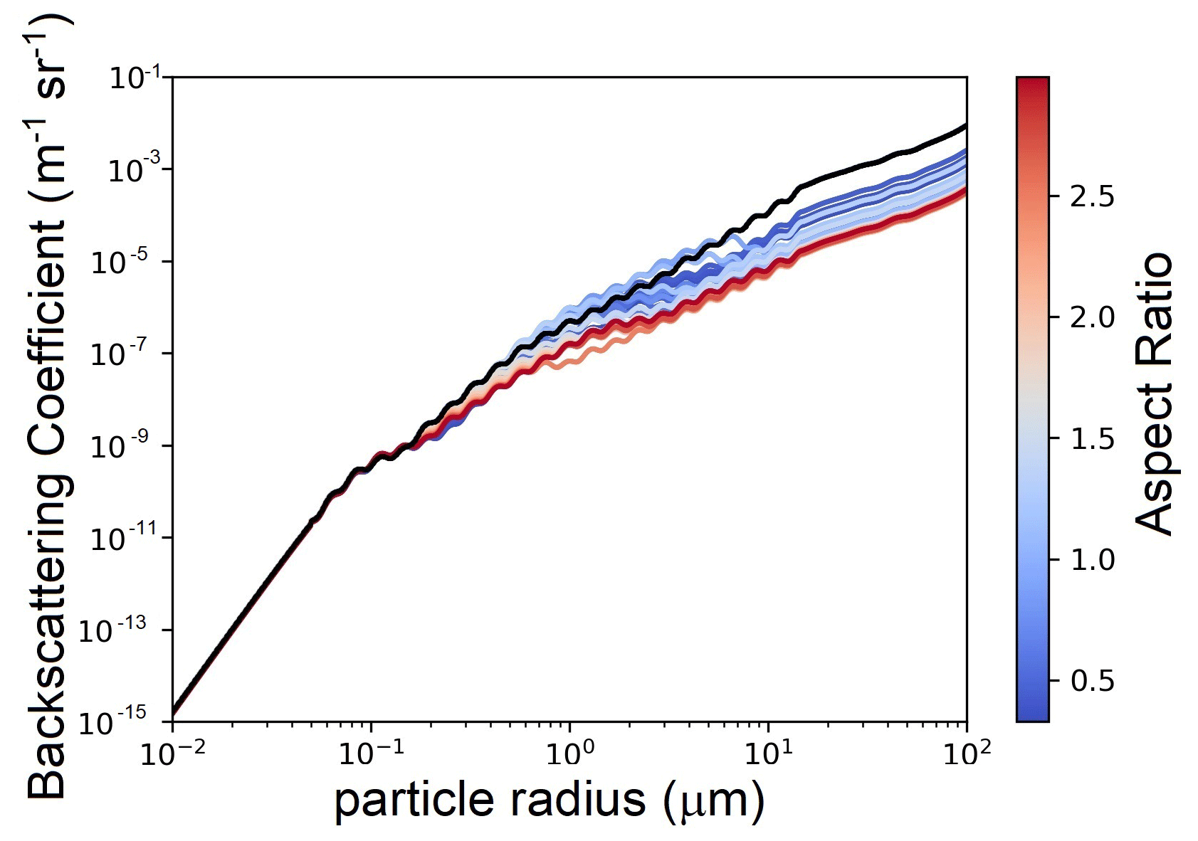
Figure A1Particle backscattering coefficient vs. particle radius for various choices of the aspect ratio. A particle concentration of 1 cm−3 has been considered. The black line refers to Mie computations (AR =1). For particle radii below 14 µm, the computations were performed with the GRASP package. Beyond 14 µm, for every given AR, the backscattering coefficients have been computed from Mie backscattering efficiencies, suitably rescaled with a constant factor. This scaling factor was chosen to make the scaled Mie efficiency overlap with the GRASP T-matrix efficiency in the particle radius dimensional region from 5 to 14 µm (60–180 size parameters).
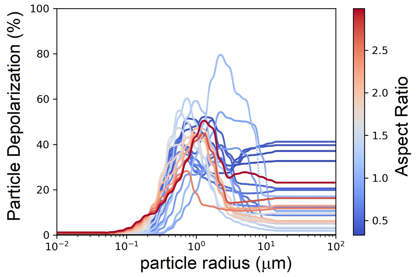
Figure A2Particle depolarization vs. particle radius for various choices of the aspect ratio. The black zero-depolarization line refers to Mie computations (AR =1). For particle radii below 14 µm, the computations were performed with the GRASP package. Beyond 14 µm, for every given AR, the depolarization of the particles was set at its constant, asymptotic value, computed as its mean over the particle radius dimensional region from 5 to 14 µm (60–180 size parameters).
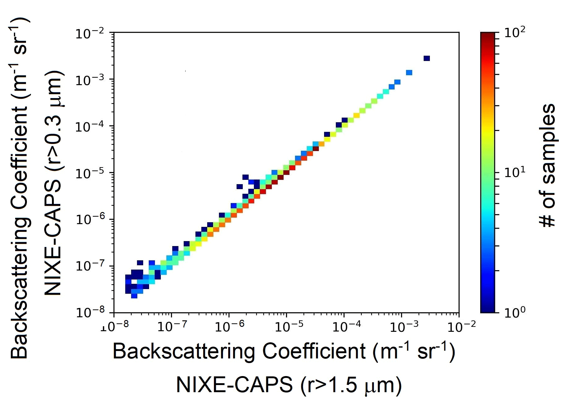
Figure A3A 2D histogram of the backscattering coefficient computed with PSD with lower size limits of 0.3 µm (y axis) and 1.5 µm (x axis). A spherical ice approximation has been used in the computation.
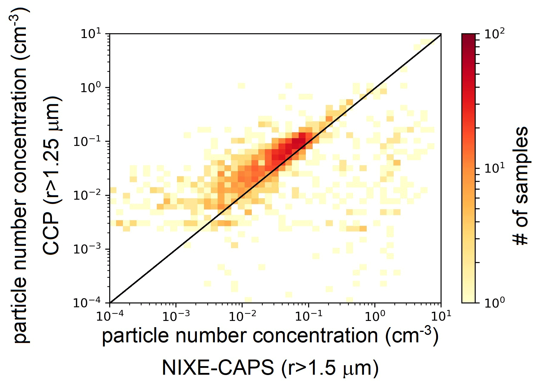
Figure A4A 2D histogram of the particle concentration Nice computed from PSD from NIXE-CAPS (x axis) and CCP (y axis). For NIXE-CAPS, only particles with a lower size limit of 1.5 µm have been considered.
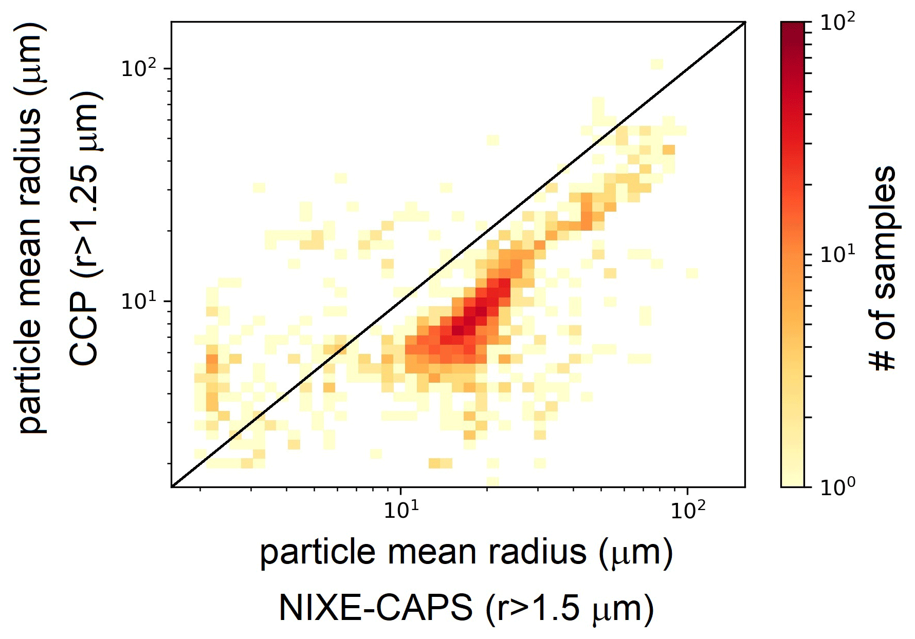
Figure A5A 2D histogram of the particle mean radius Rmean computed from PSD from NIXE-CAPS (x axis) and CCP (y axis). For NIXE-CAPS, only particles with a lower size limit of 1.5 µm have been considered.
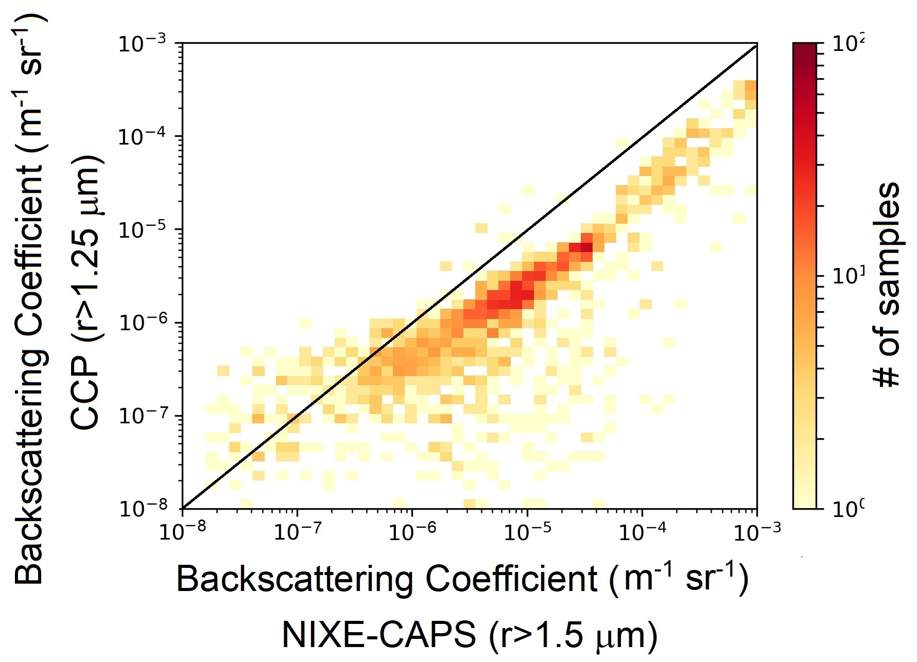
Figure A6A 2D histogram of the backscattering coefficient computed from PSD from NIXE-CAPS (x axis) and CCP (y axis). For NIXE-CAPS, only particles with a lower size limit of 1.5 µm have been considered. The computation was performed with Mie scattering codes.
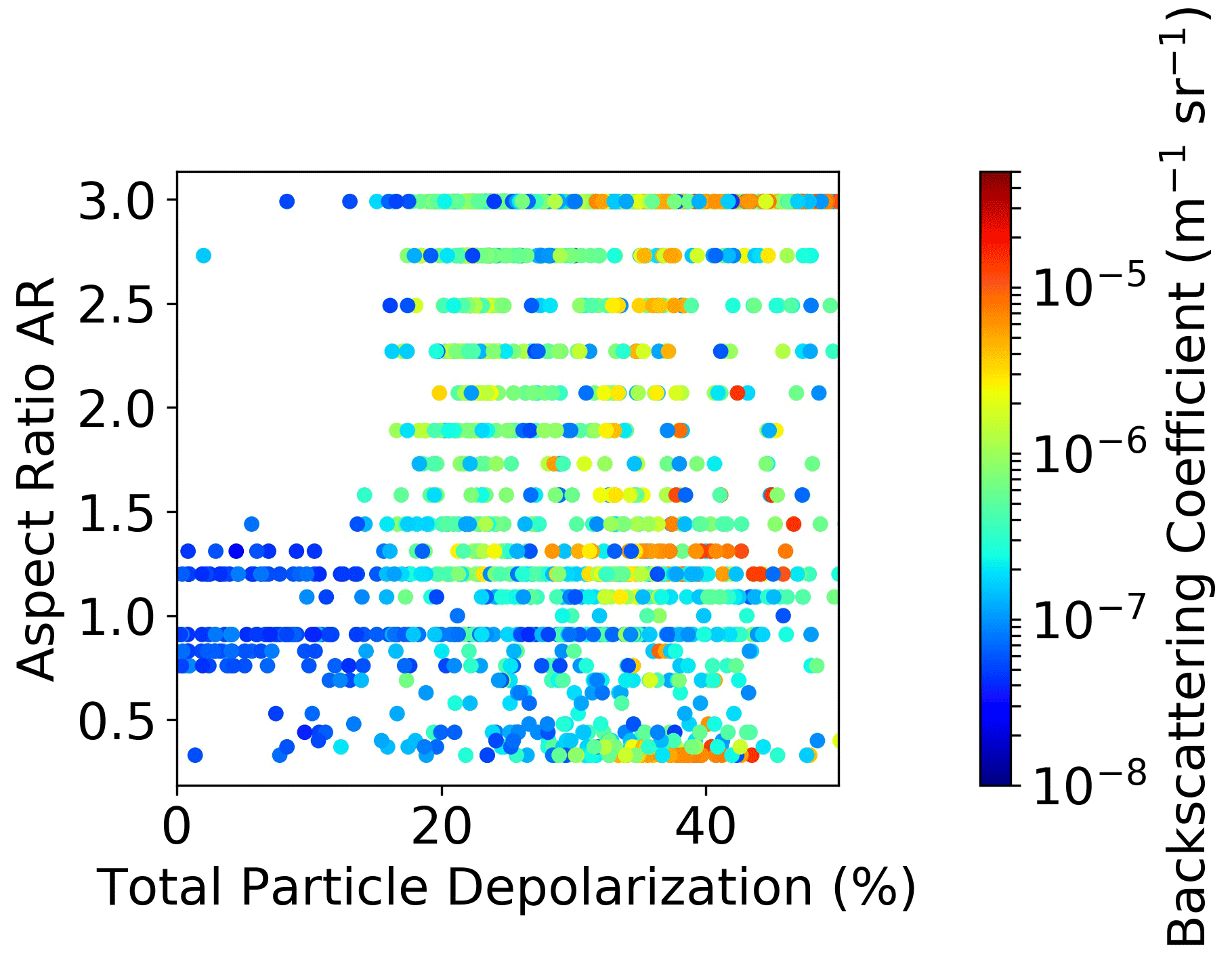
Figure A7Scatterplot of the total particle depolarization vs. the aspect ratio, color coded in terms of the backscatter coefficient.
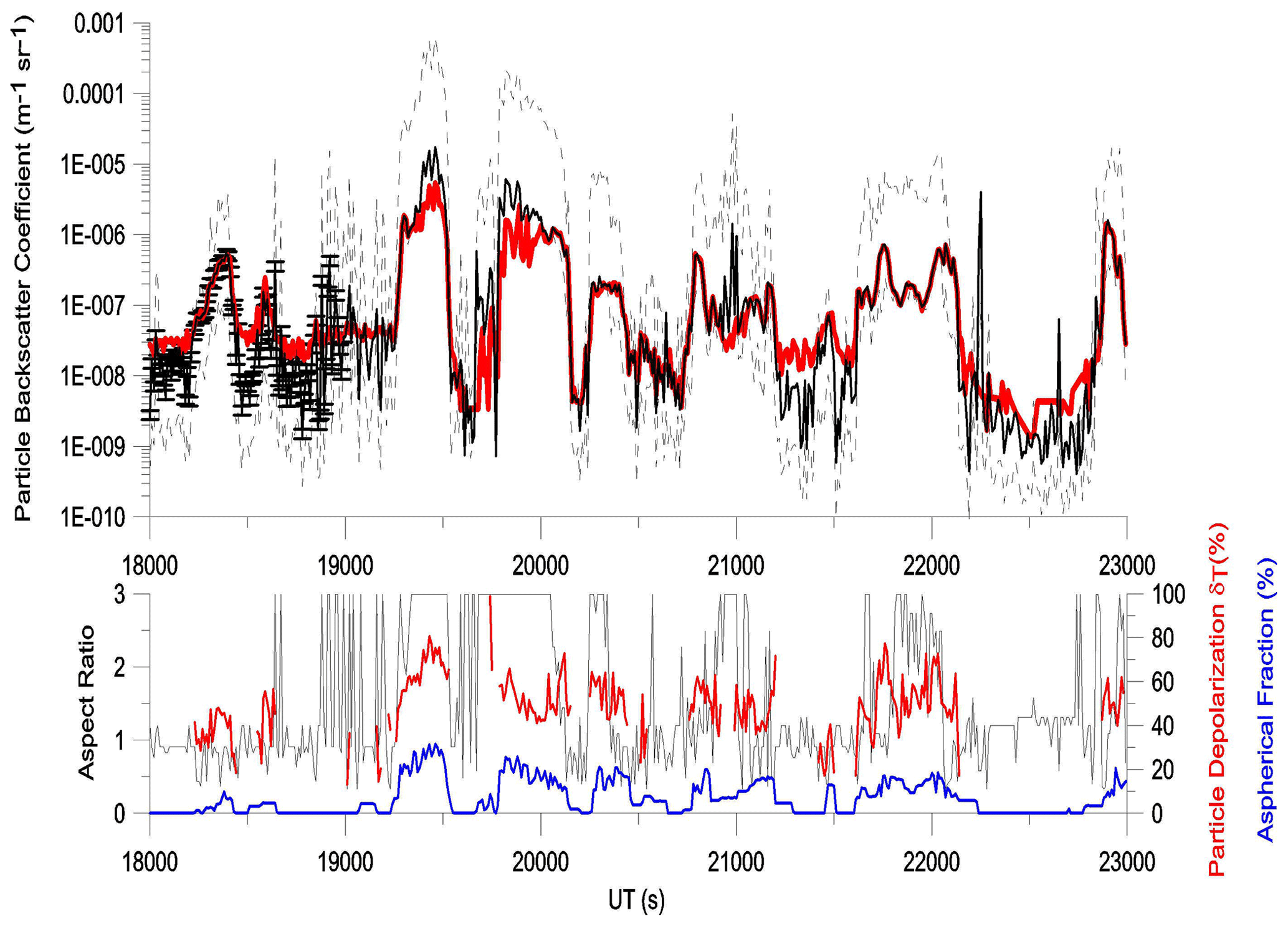
Figure A8The red line represents the time series of the particle backscattering coefficient β measured by MAS on 10 August 2017, and the solid black line represents βNC corresponding to the best match between measured δ and computed (not displayed). Error bars are reported in the first part of the curve. The dashed black lines represent maximum and minimum values of the optical-modeling values. Lower panel: the red line represents the particle depolarization measured by MAS, the blue line represents the particle aspherical fraction measured by NIXE-CAPS, and the black line represents the AF values of the best match between measured δ and computed .
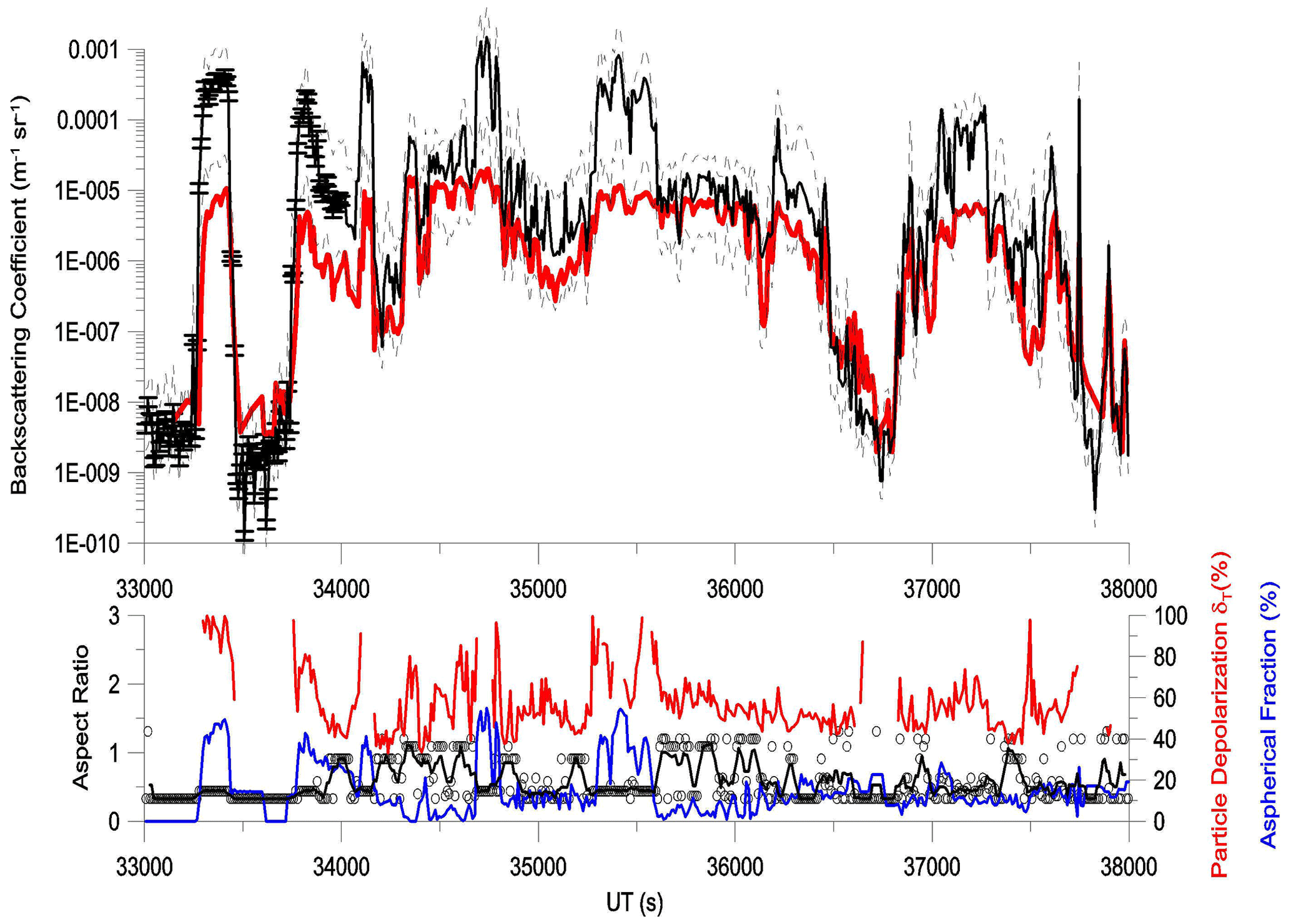
Figure A9The red line represents the time series of the particle backscattering coefficient β measured by MAS on 10 August 2017, and the solid black line represents βNC corresponding to the best match between measured δ and computed (not displayed). Error bars are reported in the first part of the curve. The dashed black lines represent the maximum and minimum values of the optical-modeling values. Lower panel: the red line represents the particle depolarization measured by MAS, the blue line represents the particle aspherical fraction measured by NIXE-CAPS, and the black line represents the AF values of the best match between measured δ and computed .
In Fig. A10, we show a 2D histogram of the backscattering coefficient computed with PSD with lower size limits of 0.3 µm (y axis) and a1.5 µm (x axis).
In Fig. A10, we show a 2D histogram of particle AF (y axis) vs. particle depolarization (x axis).
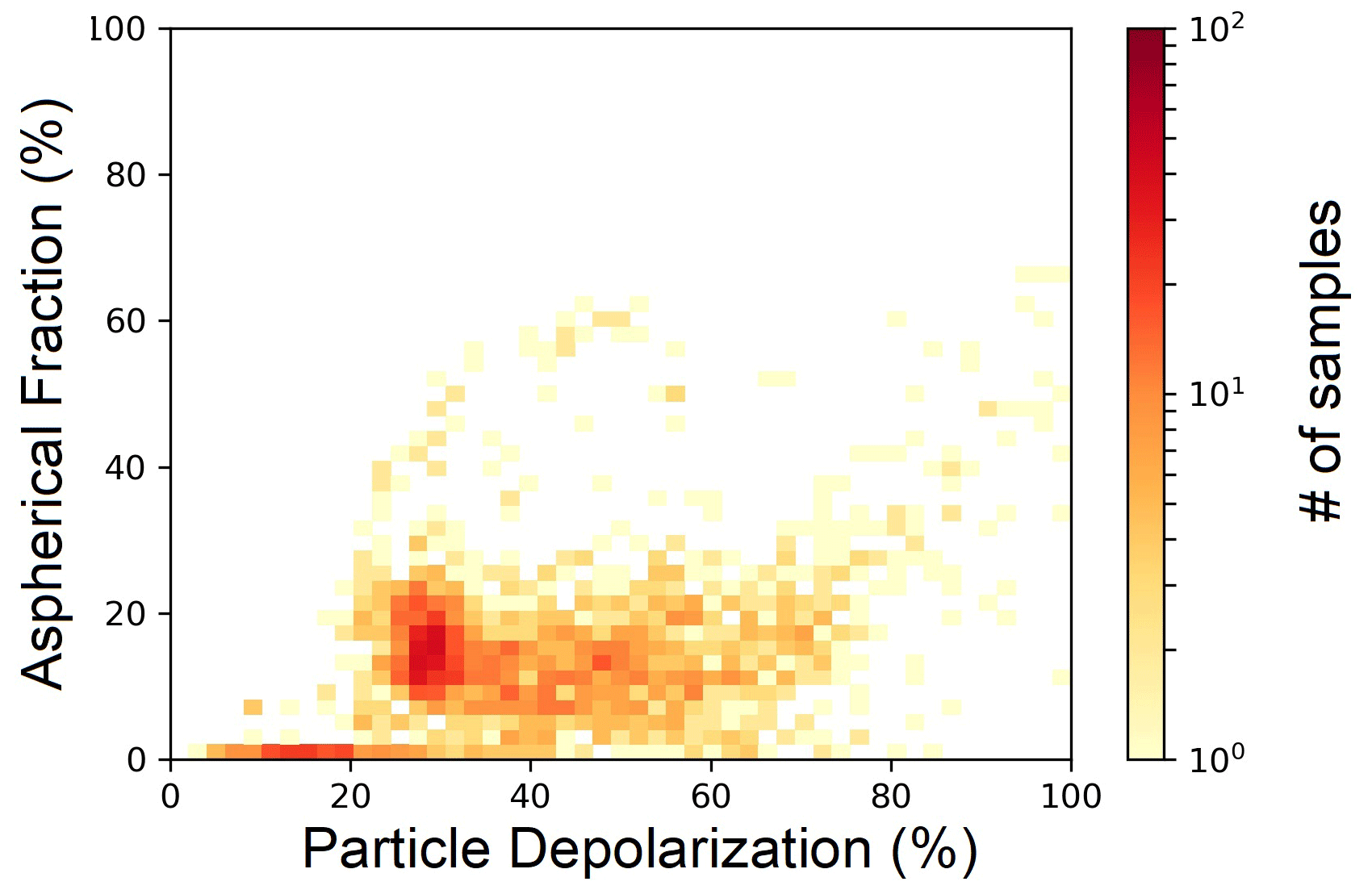
Figure A10A 2D histogram of particle aspherical fraction (y axis) vs. particle depolarization (x axis).
List of abbreviations used in the text
| Abbreviation | Definition |
| AF | Aspherical factor |
| AR | Aspect ratio |
| BR | Backscatter ratio |
| β | Backscattering coefficient |
| CALIOP | Cloud and Aerosol Lidar with Orthogonal Polarization |
| CALIPSO | Cloud-Aerosol Lidar and Infrared Pathfinder Satellite Observation |
| CAS-DPOL | Cloud and Aerosol Spectrometer with detector for polarization |
| CCP | Cloud Combination Probe |
| CDP | Cloud Droplet Probe |
| ChiWIS | Chicago Water Isotope |
| CIPgs | Cloud Imaging Probe gray scale |
| δ | Depolarization |
| DDA | Discrete dipole approximation |
| DMTs | Droplet Measurement Technologies |
| ERA5 | ECMWF Reanalysis version 5 |
| FISH | Fast In situ Stratospheric Hygrometer |
| FLASH | FLuorescent Airborne Stratospheric Hygrometer |
| GOIE | Geometric optics integral equation |
| GOM | Geometric optics method |
| GRASP | Generalized Retrieval of Aerosol and Surface Properties |
| IGOM | Improved geometric optics method |
| FDTD | Finite-difference time domain |
| IIR | Infrared imaging radiometer |
| IWC | Ice water content |
| Nice | Ice particle concentration |
| MAL | Miniature Aerosol Lidar |
| MAS | Multiwavelength Aerosol Scatterometer |
| NASA | National Aeronautics and Space Administration |
| NIXE-CAPS | New Ice eXpEriment – Cloud and Aerosol Particle Spectrometer |
| PSD | Particle size distribution |
| Reff | Effective radius |
| Rmean | Mean radius |
| RECONCILE | Reconciliation of essential process parameters for enhanced predictability of Arctic stratospheric ozone loss and climate interactions |
| TTL | Tropical tropopause layer |
| σ | Extinction coefficient |
| SAD | Surface area density |
| VD | Volume density |
Water measurements (FLASH and FISH), meteorological data from UCSE and TDC, and MAS backscatter and particle measurements from NIXE-CAPS from the StratoClim aircraft campaign are available on the HALO database at https://halo-db.pa.op.dlr.de/mission/101 (DLR, 2022). Particle measurements from CCP are available upon request to the Principal Investigators. Lidar measurements from MAL are available upon request to the PI. Analysis and plotting scripts for this paper are available upon request to the corresponding author.
MS, LDL, FC, and GDD prepared the MAS for campaign activity. FC performed and processed the MAS measurements. LL did the analysis scripts for data comparison. SK performed and processed the FLASH measurements. CR, AA, NS, and MK performed and processed the FISH and NIXE-CAPS measurements. SB and MP performed and processed the CCP measurements. RW contributed to the collection of the particle datasets. SB and FC conceived and planned the study. FC performed the analysis, prepared the figures, and drafted the paper. All the authors commented on the paper.
The contact author has declared that none of the authors has any competing interests.
Publisher’s note: Copernicus Publications remains neutral with regard to jurisdictional claims in published maps and institutional affiliations.
This article is part of the special issue “StratoClim stratospheric and upper tropospheric processes for better climate predictions (ACP/AMT inter-journal SI)”. It is not associated with a conference.
We gratefully thank the StratoClim coordination team and the Myasishchev Design Bureau for successfully conducting the field campaign. This research has been supported by the StratoClim project of the European Community's Seventh Framework Programme (project no. FP7/2007–2013) under grant agreement no. 603557 and with internal funds of the Max Planck Institute for Chemistry. Francesco Cairo is grateful to the MPI for Chemistry for supporting his sabbatical stay in Mainz, during which the study behind this publication was initiated. Sergey Khaykin's work was partly supported by the Agence Nationale de la Recherche TTL-Xing ANR-17-CE01-0015 project.
This research has been supported by the FP7 Environment Seventh Framework Programme (STRATOCLIM (grant no. 603557)).
This paper was edited by Gabriele Stiller and reviewed by two anonymous referees.
Adachi, H., Shibata, T., Iwasaka, Y., and Fujiwara, M.: Calibration method for the lidar-observed stratospheric depolarization ratio in the presence of liquid aerosol particles, Appl. Optics, 40, 6587–6595, https://doi.org/10.1364/AO.40.006587, 2001. a
Afchine, A., Rolf, C., Costa, A., Spelten, N., Riese, M., Buchholz, B., Ebert, V., Heller, R., Kaufmann, S., Minikin, A., Voigt, C., Zöger, M., Smith, J., Lawson, P., Lykov, A., Khaykin, S., and Krämer, M.: Ice particle sampling from aircraft – influence of the probing position on the ice water content, Atmos. Meas. Tech., 11, 4015–4031, https://doi.org/10.5194/amt-11-4015-2018, 2018. a, b, c
AMS (American Meteorological Society): Cirrus, Glossary of Meteorology, http://glossary.ametsoc.org/wiki/cirrus (last access: 18 October 2023), 2023. a
Austin, R. T., Heymsfield, A. J., and Stephens, G. L.: Retrieval of ice cloud microphysical parameters using the CloudSat millimeter-wave radar and temperature, J. Geophys. Res.-Atmos., 114, D00A23, https://doi.org/10.1029/2008JD010049, 2009. a
Avery, M., Winker, D., Heymsfield, A., Vaughan, M., Young, S., Hu, Y., and Trepte, C.: Cloud ice water content retrieved from the CALIOP space-based lidar, Geophys. Res. Lett., 39, L05808, https://doi.org/10.1029/2011GL050545, 2012. a, b, c, d
Bailey, M. P. and Hallett, J.: A Comprehensive Habit Diagram for Atmospheric Ice Crystals: Confirmation from the Laboratory, AIRS II, and Other Field Studies, J. Atmos. Sci., 66, 2888–2899, https://doi.org/10.1175/2009JAS2883.1, 2009. a
Balmes, K. A., Fu, Q., and Thorsen, T. J.: Differences in Ice Cloud Optical Depth From CALIPSO and Ground-Based Raman Lidar at the ARM SGP and TWP Sites, J. Geophys. Res.-Atmos., 124, 1755–1778, https://doi.org/10.1029/2018JD028321, 2019. a, b
Baran, A. J., Francis, P. N., Havemann, S., and Yang, P.: A study of the absorption and extinction properties of hexagonal ice columns and plates in random and preferred orientation, using exact T-matrix theory and aircraft observations of cirrus, J. Quant. Spectrosc. Ra., 70, 505–518, https://doi.org/10.1016/S0022-4073(01)00025-5, 2001. a
Baumgardner, D., Abel, S. J., Axisa, D., Cotton, R., Crosier, J., Field, P., Gurganus, C., Heymsfield, A., Korolev, A., Krämer, M., Lawson, P., McFarquhar, G., Ulanowski, Z., and Um, J.: Cloud Ice Properties: In Situ Measurement Challenges, Meteor. Mon., 58, 9.1–9.23, https://doi.org/10.1175/AMSMONOGRAPHS-D-16-0011.1, 2017. a
Berendsen, H. J. C.: A Student's Guide to Data and Error Analysis, Student's Guides, Cambridge University Press, https://doi.org/10.1017/CBO9780511921247, 2011. a
Bi, L. and Yang, P.: Accurate simulation of the optical properties of atmospheric ice crystals with the invariant imbedding T-matrix method, J. Quant. Spectrosc. Ra., 138, 17–35, https://doi.org/10.1016/j.jqsrt.2014.01.013, 2014. a
Bohren, C. F. and Huffman, D. R.: Absorption and scattering of light by small particles, John Wiley & Sons, ISBN: 3527618163, 9783527618163 2008. a
Borrmann, S. and Luo, B.: Application of the T-matrix method to the measurement of aspherical (ellipsoidal) particles with forward scattering optical particle counters, J. Aerosol Sci., 31, 789–799, https://doi.org/10.1016/S0021-8502(99)00563-7, 2000. a
Boucher, O., Randall, D., Artaxo, P., Bretherton, C., Feingold, G., Forster, P., Kerminen, V.-M., Kondo, Y., Liao, H., Lohmann, U., Rasch, P., Satheesh, S. K., Sherwood, S., Stevens, B., and Zhang, X. Y.: Clouds and aerosols, Cambridge University Press, Cambridge, UK, 571–657, https://doi.org/10.1017/CBO9781107415324.016, 2013. a
Cairo, F., Donfrancesco, G. D., Adriani, A., Pulvirenti, L., and Fierli, F.: Comparison of various linear depolarization parameters measured by lidar, Appl. Optics, 38, 4425–4432, https://doi.org/10.1364/AO.38.004425, 1999. a, b
Cairo, F., Adriani, A., Viterbini, M., Di Donfrancesco, G., Mitev, V., Matthey, R., Bastiano, M., Redaelli, G., Dragani, R., Ferretti, R., Rizi, V., Paolucci, T., Bernardini, L., Cacciani, M., Pace, G., and Fiocco, G.: Polar stratospheric clouds observed during the Airborne Polar Experiment–Geophysica Aircraft in Antarctica (APE-GAIA) campaign, J. Geophys. Res.-Atmos., 109, D07204, https://doi.org/10.1029/2003JD003930, 2004. a
Cairo, F., Di Donfrancesco, G., Snels, M., Fierli, F., Viterbini, M., Borrmann, S., and Frey, W.: A comparison of light backscattering and particle size distribution measurements in tropical cirrus clouds, Atmos. Meas. Tech., 4, 557–570, https://doi.org/10.5194/amt-4-557-2011, 2011. a, b, c, d
Cairo, F., De Muro, M., Snels, M., Di Liberto, L., Bucci, S., Legras, B., Kottayil, A., Scoccione, A., and Ghisu, S.: Lidar observations of cirrus clouds in Palau (7∘33′ N, 134∘48′ E), Atmos. Chem. Phys., 21, 7947–7961, https://doi.org/10.5194/acp-21-7947-2021, 2021. a
Cairo, F., Deshler, T., Di Liberto, L., Scoccione, A., and Snels, M.: A study of optical scattering modelling for mixed-phase polar stratospheric clouds, Atmos. Meas. Tech., 16, 419–431, https://doi.org/10.5194/amt-16-419-2023, 2023. a
Campbell, J. R., Lolli, S., Lewis, J. R., Gu, Y., and Welton, E. J.: Daytime cirrus cloud top-of-atmosphere radiative forcing properties at a midlatitude site and their global consequence, J. Appl. Meteorol. Clim., 55, 1667–1679, 2016. a
Chen, W.-N., Chiang, C.-W., and Nee, J.-B.: Lidar ratio and depolarization ratio for cirrus clouds, Appl. Optics, 41, 6470–6476, https://doi.org/10.1364/AO.41.006470, 2002. a
Collis, R. T. H. and Russell, P. B.: Lidar measurement of particles and gases by elastic backscattering and differential absorption, in: Laser Monitoring of the Atmosphere. Topics in Applied Physics, Vol. 14, edited by: Hinkley, E. D., Springer, Berlin, Heidelberg, https://doi.org/10.1007/3-540-07743-X_18, 1976. a
Corti, T., Luo, B., De Reus, M., Brunner, D., Cairo, F., Mahoney, M., Martucci, G., Matthey, R., Mitev, V., dos Santos, F., Schiller, C., Shur, G., Sitnikov, N. M., Spelten, N., Vössing, H. J., Borrmann, S., and Peter, T.: Unprecedented evidence for deep convection hydrating the tropical stratosphere, Geophys. Res. Lett., 35, L10810, https://doi.org/10.1029/2008GL033641, 2008. a
Costa, A., Meyer, J., Afchine, A., Luebke, A., Günther, G., Dorsey, J. R., Gallagher, M. W., Ehrlich, A., Wendisch, M., Baumgardner, D., Wex, H., and Krämer, M.: Classification of Arctic, midlatitude and tropical clouds in the mixed-phase temperature regime, Atmos. Chem. Phys., 17, 12219–12238, https://doi.org/10.5194/acp-17-12219-2017, 2017. a, b, c
Delanoë, J. and Hogan, R. J.: Combined CloudSat-CALIPSO-MODIS retrievals of the properties of ice clouds, J. Geophys. Res.-Atmos., 115, D00H29, https://doi.org/10.1029/2009JD012346, 2010. a
Deshler, T., Nardi, B., Adriani, A., Cairo, F., Hansen, G., Fierli, F., Hauchecorne, A., and Pulvirenti, L.: Determining the index of refraction of polar stratospheric clouds above Andoya (69∘ N) by combining size-resolved concentration and optical scattering measurements, J. Geophys. Res.-Atmos., 105, 3943–3953, 2000. a
DLR (German Aerospace Center): Mission: STRATOCLIM, HALO database [data set], https://halo-db.pa.op.dlr.de/mission/101 (last access: 1 May 2022), 2022. a
Dubovik, O., Sinyuk, A., Lapyonok, T., Holben, B. N., Mishchenko, M., Yang, P., Eck, T. F., Volten, H., Muñoz, O., Veihelmann, B., van der Zande, W. J., Leon, J.-F., Sorokin, M., and Slutsker, I.: Application of spheroid models to account for aerosol particle nonsphericity in remote sensing of desert dust, J. Geophys. Res., 111, D11208, https://doi.org/10.1029/2005JD006619, 2006. a, b
Dubovik, O., Lapyonok, T., Litvinov, P., Herman, M., Fuertes, D., Ducos, F., Torres, B., Derimian, Y., Huang, X., Lopatin, A., Chaikovsky, A., Aspetsberger, M., and Federspiel, C.: GRASP: a versatile algorithm for characterizing the atmosphere, SPIE Newsroom, https://doi.org/10.1117/2.1201408.005558, 2014. a
Frey, W., Borrmann, S., Kunkel, D., Weigel, R., de Reus, M., Schlager, H., Roiger, A., Voigt, C., Hoor, P., Curtius, J., Krämer, M., Schiller, C., Volk, C. M., Homan, C. D., Fierli, F., Di Donfrancesco, G., Ulanovsky, A., Ravegnani, F., Sitnikov, N. M., Viciani, S., D'Amato, F., Shur, G. N., Belyaev, G. V., Law, K. S., and Cairo, F.: In situ measurements of tropical cloud properties in the West African Monsoon: upper tropospheric ice clouds, Mesoscale Convective System outflow, and subvisual cirrus, Atmos. Chem. Phys., 11, 5569–5590, https://doi.org/10.5194/acp-11-5569-2011, 2011. a, b
Frey, W., Borrmann, S., Fierli, F., Weigel, R., Mitev, V., Matthey, R., Ravegnani, F., Sitnikov, N. M., Ulanovsky, A., and Cairo, F.: Tropical deep convective life cycle: Cb-anvil cloud microphysics from high-altitude aircraft observations, Atmos. Chem. Phys., 14, 13223–13240, https://doi.org/10.5194/acp-14-13223-2014, 2014. a
Fu, Q.: A New Parameterization of an Asymmetry Factor of Cirrus Clouds for Climate Models, J. Atmos. Sci., 64, 4140–4150, https://doi.org/10.1175/2007JAS2289.1, 2007. a
Fueglistaler, S., Dessler, A. E., Dunkerton, T. J., Folkins, I., Fu, Q., and Mote, P. W.: Tropical tropopause layer, Rev. Geophys., 47, RG1004, https://doi.org/10.1029/2008RG000267, 2009. a
Fujiwara, M., Iwasaki, S., Shimizu, A., Inai, Y., Shiotani, M., Hasebe, F., Matsui, I., Sugimoto, N., Okamoto, H., Nishi, N., Hamada, A., Sakazaki, T., and Yoneyama, K.: Cirrus observations in the tropical tropopause layer over the western Pacific, J. Geophys. Res.-Atmos., 114, D09304, https://doi.org/10.1029/2008JD011040, 2009. a
Groth, S. P., Baran, A. J., Betcke, T., Havemann, S., and Śmigaj, W.: The boundary element method for light scattering by ice crystals and its implementation in BEM++, J. Quant. Spectrosc. Ra., 167, 40–52, 2015. a
Grulich, L., Weigel, R., Hildebrandt, A., Wand, M., and Spichtinger, P.: Automatic shape detection of ice crystals, J. Comput. Sci.-Neth., 54, 101429, https://doi.org/10.1016/j.jocs.2021.101429, 2021. a
Guignard, A., Stubenrauch, C. J., Baran, A. J., and Armante, R.: Bulk microphysical properties of semi-transparent cirrus from AIRS: a six year global climatology and statistical analysis in synergy with geometrical profiling data from CloudSat-CALIPSO, Atmos. Chem. Phys., 12, 503–525, https://doi.org/10.5194/acp-12-503-2012, 2012. a
He, Q., LI, C., Ma, J., Wang, H., Shi, G., Liang, Z., Luan, Q., Geng, F., and Zhou, a.: The Properties and Formation of Cirrus Clouds over the Tibetan Plateau Based on Summertime Lidar Measurements, J. Atmos. Sci., 70, https://doi.org/10.1175/JAS-D-12-0171.1, 2012. a
Heymsfield, A., Winker, D., Avery, M., Vaughan, M., Diskin, G., Deng, M., Mitev, V., and Matthey, R.: Relationships between Ice Water Content and Volume Extinction Coefficient from In Situ Observations for Temperatures from 0∘ to −86 ∘C: Implications for Spaceborne Lidar Retrievals, J. Appl. Meteorol. Clim., 53, 479–505, https://doi.org/10.1175/JAMC-D-13-087.1, 2014. a, b, c, d, e
Heymsfield, A. J., Winker, D., and van Zadelhoff, G.-J.: Extinction-ice water content-effective radius algorithms for CALIPSO, Geophys. Res. Lett., 32, https://doi.org/10.1029/2005GL022742, 2005. a, b, c
Immler, F., Krüger, K., Fujiwara, M., Verver, G., Rex, M., and Schrems, O.: Correlation between equatorial Kelvin waves and the occurrence of extremely thin ice clouds at the tropical tropopause, Atmos. Chem. Phys., 8, 4019–4026, https://doi.org/10.5194/acp-8-4019-2008, 2008. a
Ishimoto, H., Masuda, K., Mano, Y., Orikasa, N., and Uchiyama, A.: Optical modeling of irregularly shaped ice particles in convective cirrus, in: AIP Conference Proceedings, American Institute of Physics, 1531, 184–187, 2013. a
Jensen, E. J., Toon, O. B., Pfister, L., and Selkirk, H. B.: Dehydration of the upper troposphere and lower stratosphere by subvisible cirrus clouds near the tropical tropopause, Geophys. Res. Lett., 23, 825–828, https://doi.org/10.1029/96GL00722, 1996. a
Khaykin, S. M., Engel, I., Vömel, H., Formanyuk, I. M., Kivi, R., Korshunov, L. I., Krämer, M., Lykov, A. D., Meier, S., Naebert, T., Pitts, M. C., Santee, M. L., Spelten, N., Wienhold, F. G., Yushkov, V. A., and Peter, T.: Arctic stratospheric dehydration – Part 1: Unprecedented observation of vertical redistribution of water, Atmos. Chem. Phys., 13, 11503–11517, https://doi.org/10.5194/acp-13-11503-2013, 2013. a
Khaykin, S. M., Moyer, E., Krämer, M., Clouser, B., Bucci, S., Legras, B., Lykov, A., Afchine, A., Cairo, F., Formanyuk, I., Mitev, V., Matthey, R., Rolf, C., Singer, C. E., Spelten, N., Volkov, V., Yushkov, V., and Stroh, F.: Persistence of moist plumes from overshooting convection in the Asian monsoon anticyclone, Atmos. Chem. Phys., 22, 3169–3189, https://doi.org/10.5194/acp-22-3169-2022, 2022. a, b
Klingebiel, M., de Lozar, A., Molleker, S., Weigel, R., Roth, A., Schmidt, L., Meyer, J., Ehrlich, A., Neuber, R., Wendisch, M., and Borrmann, S.: Arctic low-level boundary layer clouds: in situ measurements and simulations of mono- and bimodal supercooled droplet size distributions at the top layer of liquid phase clouds, Atmos. Chem. Phys., 15, 617–631, https://doi.org/10.5194/acp-15-617-2015, 2015. a, b
Konoshonkin, A., Borovoi, A., Kustova, N., Okamoto, H., Ishimoto, H., Grynko, Y., and Förstner, J.: Light scattering by ice crystals of cirrus clouds: From exact numerical methods to physical-optics approximation, J. Quant. Spectrosc. Ra., 195, 132–140, https://doi.org/10.1016/j.jqsrt.2016.12.024, 2017a. a
Konoshonkin, A., Borovoi, A., Kustova, N., and Reichardt, J.: Power laws for backscattering by ice crystals of cirrus clouds, Opt. Express, 25, 22341–22346, https://doi.org/10.1364/OE.25.022341, 2017b. a
Krämer, M., Schiller, C., Afchine, A., Bauer, R., Gensch, I., Mangold, A., Schlicht, S., Spelten, N., Sitnikov, N., Borrmann, S., de Reus, M., and Spichtinger, P.: Ice supersaturations and cirrus cloud crystal numbers, Atmos. Chem. Phys., 9, 3505–3522, https://doi.org/10.5194/acp-9-3505-2009, 2009. a, b
Krämer, M., Rolf, C., Luebke, A., Afchine, A., Spelten, N., Costa, A., Meyer, J., Zöger, M., Smith, J., Herman, R. L., Buchholz, B., Ebert, V., Baumgardner, D., Borrmann, S., Klingebiel, M., and Avallone, L.: A microphysics guide to cirrus clouds – Part 1: Cirrus types, Atmos. Chem. Phys., 16, 3463–3483, https://doi.org/10.5194/acp-16-3463-2016, 2016. a, b, c
Krämer, M., Rolf, C., Spelten, N., Afchine, A., Fahey, D., Jensen, E., Khaykin, S., Kuhn, T., Lawson, P., Lykov, A., Pan, L. L., Riese, M., Rollins, A., Stroh, F., Thornberry, T., Wolf, V., Woods, S., Spichtinger, P., Quaas, J., and Sourdeval, O.: A microphysics guide to cirrus – Part 2: Climatologies of clouds and humidity from observations, Atmos. Chem. Phys., 20, 12569–12608, https://doi.org/10.5194/acp-20-12569-2020, 2020. a, b, c, d, e
Lamraoui, F., Krämer, M., Afchine, A., Sokol, A. B., Khaykin, S., Pandey, A., and Kuang, Z.: Sensitivity of convectively driven tropical tropopause cirrus properties to ice habits in high-resolution simulations, Atmos. Chem. Phys., 23, 2393–2419, https://doi.org/10.5194/acp-23-2393-2023, 2023. a
Lawson, R. P., Woods, S., Jensen, E., Erfani, E., Gurganus, C., Gallagher, M., Connolly, P., Whiteway, J., Baran, A. J., May, P., Heymsfield, A., Schmitt, C. G., McFarquhar, G., Um, J., Protat, A., Bailey, M., Lance, S., Muehlbauer, A., Stith, J., Korolev, A., Toon, O. B., and Krämer, M.: A Review of Ice Particle Shapes in Cirrus formed In Situ and in Anvils, J. Geophys. Res.-Atmos., 124, 10049–10090, https://doi.org/10.1029/2018JD030122, 2019. a
Liou, K. and Yang, P.: Light Scattering by Ice Crystals: Fundamentals and Applications, Cambridge University Press, Cambridge, https://doi.org/10.1017/CBO9781139030052, 2016. a
Liu, C., Panetta, R. L., and Yang, P.: Application of the pseudo-spectral time domain method to compute particle single-scattering properties for size parameters up to 200, J. Quant. Spectrosc. Ra., 113, 1728–1740, 2012. a
Liu, L. and Mishchenko, M. I.: Constraints on PSC particle microphysics derived from lidar observations, J. Quant. Spectrosc. Ra., 70, 817–831, 2001. a, b
Liu, L., Mishchenko, M. I., Cairns, B., Carlson, B. E., and Travis, L. D.: Modeling single-scattering properties of small cirrus particles by use of a size-shape distribution of ice spheroids and cylinders, J. Quant. Spectrosc. Ra., 101, 488–497, https://doi.org/10.1016/j.jqsrt.2006.02.040, 2006. a
Lolli, S.: Daytime top-of-the-atmosphere cirrus cloud radiative forcing properties at Singapore, J. Appl. Meteorol. Clim., 56, 1249–1257, 2017. a
Luebke, A. E., Avallone, L. M., Schiller, C., Meyer, J., Rolf, C., and Krämer, M.: Ice water content of Arctic, midlatitude, and tropical cirrus – Part 2: Extension of the database and new statistical analysis, Atmos. Chem. Phys., 13, 6447–6459, https://doi.org/10.5194/acp-13-6447-2013, 2013. a
Luebke, A. E., Afchine, A., Costa, A., Grooß, J.-U., Meyer, J., Rolf, C., Spelten, N., Avallone, L. M., Baumgardner, D., and Krämer, M.: The origin of midlatitude ice clouds and the resulting influence on their microphysical properties, Atmos. Chem. Phys., 16, 5793–5809, https://doi.org/10.5194/acp-16-5793-2016, 2016. a, b
Luo, B. P., Peter, T., Fueglistaler, S., Wernli, H., Wirth, M., Kiemle, C., Flentje, H., Yushkov, V. A., Khattatov, V., Rudakov, V., Thomas, A., Borrmann, S., Toci, G., Mazzinghi, P., Beuermann, J., Schiller, C., Cairo, F., Di Donfrancesco, G., Adriani, A., Volk, C. M., Strom, J., Noone, K., Mitev, V., MacKenzie, R. A., Carslaw, K. S., Trautmann, T., Santacesaria, V., and Stefanutti, L.: Dehydration potential of ultrathin clouds at the tropical tropopause, Geophys. Res. Lett., 30, 1557, https://doi.org/10.1029/2002GL016737, 2003. a
Lynch, D.: Cirrus clouds: Their role in climate and global change, Acta Astronaut., 38, 859–863, https://doi.org/10.1016/S0094-5765(96)00098-7, 1996. a
Lynch, D., Sassen, K., Delgenio, A., Heymsfield, A., Minnis, P., Platt, M., Quante, M., Schumann, U., and Sundqvist, H.: Cirrus, Oxford University Press, https://doi.org/10.1093/oso/9780195130720.003.0025, 2002. a
Macke, A., Mueller, J., and Raschke, E.: Single scattering properties of atmospheric ice crystals, J. Atmos. Sci., 53, 2813–2825, 1996. a
MacKenzie, A. R., Schiller, C., Peter, T., Adriani, A., Beuermann, J., Bujok, O., Cairo, F., Corti, T., DiDonfrancesco, G., Gensch, I., Kiemle, C., Krämer, M., Kröger, C., Merkulov, S., Oulanovsky, A., Ravegnani, F., Rohs, S., Rudakov, V., Salter, P., Santacesaria, V., Stefanutti, L., and Yushkov, V.: Tropopause and hygropause variability over the equatorial Indian Ocean during February and March 1999, J. Geophys. Res.-Atmos., 111, D18112, https://doi.org/10.1029/2005JD006639, 2006. a
Mahnke, C., Weigel, R., Cairo, F., Vernier, J.-P., Afchine, A., Krämer, M., Mitev, V., Matthey, R., Viciani, S., D'Amato, F., Ploeger, F., Deshler, T., and Borrmann, S.: The Asian tropopause aerosol layer within the 2017 monsoon anticyclone: microphysical properties derived from aircraft-borne in situ measurements, Atmos. Chem. Phys., 21, 15259–15282, https://doi.org/10.5194/acp-21-15259-2021, 2021. a
Martucci, G., Mitev, V., Matthey, R., and Makarov, V.: Compact backscatttter Lidar for cloud detection on a stratospheric aircraft, Proc. SPIE, 5979, https://doi.org/10.1117/12.627644, 2005. a
Mei, F., Wang, J., Comstock, J. M., Weigel, R., Krämer, M., Mahnke, C., Shilling, J. E., Schneider, J., Schulz, C., Long, C. N., Wendisch, M., Machado, L. A. T., Schmid, B., Krisna, T., Pekour, M., Hubbe, J., Giez, A., Weinzierl, B., Zoeger, M., Pöhlker, M. L., Schlager, H., Cecchini, M. A., Andreae, M. O., Martin, S. T., de Sá, S. S., Fan, J., Tomlinson, J., Springston, S., Pöschl, U., Artaxo, P., Pöhlker, C., Klimach, T., Minikin, A., Afchine, A., and Borrmann, S.: Comparison of aircraft measurements during GoAmazon2014/5 and ACRIDICON-CHUVA, Atmos. Meas. Tech., 13, 661–684, https://doi.org/10.5194/amt-13-661-2020, 2020. a, b
Meyer, J., Rolf, C., Schiller, C., Rohs, S., Spelten, N., Afchine, A., Zöger, M., Sitnikov, N., Thornberry, T. D., Rollins, A. W., Bozóki, Z., Tátrai, D., Ebert, V., Kühnreich, B., Mackrodt, P., Möhler, O., Saathoff, H., Rosenlof, K. H., and Krämer, M.: Two decades of water vapor measurements with the FISH fluorescence hygrometer: a review, Atmos. Chem. Phys., 15, 8521–8538, https://doi.org/10.5194/acp-15-8521-2015, 2015. a
Meyer, K. and Platnick, S.: Utilizing the MODIS 1.38 µm channel for cirrus cloud optical thickness retrievals: Algorithm and retrieval uncertainties, J. Geophys. Res., 115, D24209, https://doi.org/10.1029/2010JD014872, 2010. a
Mishchenko, M. I., Travis, L. D., and Mackowski, D. W.: T-matrix computations of light scattering by nonspherical particles: A review, J. Quant. Spectrosc. Ra., 55, 535–575, https://doi.org/10.1016/0022-4073(96)00002-7, 1996. a
Mishchenko, M. I., Wielaard, D. J., and Carlson, B. E.: T-matrix computations of zenith-enhanced lidar backscatter from horizontally oriented ice plates, Geophys. Res. Lett., 24, 771–774, https://doi.org/10.1029/97GL00545, 1997. a
Mishchenko, M. I., Hovenier, J. W., and Travis, L. D.: Light scattering by nonspherical particles: theory, measurements, and applications, Elsevier, ISBN: 9780124986602, 1999. a
Mishchenko, M. I., Travis, L. D., and Lacis, A. A.: Scattering, Absorption, and Emission of Light by Small Particles, Cambridge University Press, Cambridge, ISBN: 052178252X, 9780521782524, 2002. a
Mitchell, D. L., Lawson, R. P., and Baker, B.: Understanding effective diameter and its application to terrestrial radiation in ice clouds, Atmos. Chem. Phys., 11, 3417–3429, https://doi.org/10.5194/acp-11-3417-2011, 2011. a
Mitchell, D. L., Garnier, A., Pelon, J., and Erfani, E.: CALIPSO (IIR–CALIOP) retrievals of cirrus cloud ice-particle concentrations, Atmos. Chem. Phys., 18, 17325–17354, https://doi.org/10.5194/acp-18-17325-2018, 2018. a
Mitev, V., Poole, L. R., Pitts, M. C., and Matthey, R.: Comparison Case Between CALIPSO Lidar and Mals On M55 Geophysica During Reconcile Campaign, in: 26th International Laser Radar Conference, ILRC, Porto Heli, Greece, 25–29 June 2012, 729–732, 2012. a
Molleker, S., Borrmann, S., Schlager, H., Luo, B., Frey, W., Klingebiel, M., Weigel, R., Ebert, M., Mitev, V., Matthey, R., Woiwode, W., Oelhaf, H., Dörnbrack, A., Stratmann, G., Grooß, J.-U., Günther, G., Vogel, B., Müller, R., Krämer, M., Meyer, J., and Cairo, F.: Microphysical properties of synoptic-scale polar stratospheric clouds: in situ measurements of unexpectedly large HNO3-containing particles in the Arctic vortex, Atmos. Chem. Phys., 14, 10785–10801, https://doi.org/10.5194/acp-14-10785-2014, 2014. a, b
Nakajima, T. Y., Nakajima, T., Yoshimori, K., Mishra, S. K., and Tripathi, S. N.: Development of a light scattering solver applicable to particles of arbitrary shape on the basis of the surface-integral equations method of Müller type. I. Methodology, accuracy of calculation, and electromagnetic current on the particle surface, Appl. Optics, 48, 3526–3536, 2009. a
Nazaryan, H., Mccormick, M., and Menzel, W.: Global characterization of cirrus clouds using CALIPSO data, J. Geophys. Res., 113, D16211, https://doi.org/10.1029/2007JD009481, 2008. a
Pfister, L., Selkirk, H. B., Jensen, E. J., Schoeberl, M. R., Toon, O. B., Browell, E. V., Grant, W. B., Gary, B., Mahoney, M. J., Bui, T. V., and Hintsa, E.: Aircraft observations of thin cirrus clouds near the tropical tropopause, J. Geophys. Res.-Atmos., 106, 9765–9786, https://doi.org/10.1029/2000JD900648, 2001. a
Port, M.: Flugzeuggetragene Messungen von Zirren und vereisten Wolken im Troposphären-Stratosphären-Übergangsbereich des asiatischen Sommermonsuns, PhD thesis, Fachbereich Physik, Mathematik und Informatik der Johannes Gutenberg-Universität Mainz, https://doi.org/10.25358/openscience-7538, 2021. a
Prabhakara, C., Kratz, D., Yoo, J.-M., Dalu, G., and Vernekar, A.: Optically thin cirrus clouds: Radiative impact on the warm pool, J. Quant. Spectrosc. Ra., 49, 467–483, https://doi.org/10.1016/0022-4073(93)90061-L, 1993. a
Sarkozy, L. C., Clouser, B. W., Lamb, K. D., Stutz, E. J., Saathoff, H., Möhler, O., Ebert, V., and Moyer, E. J.: The Chicago Water Isotope Spectrometer (ChiWIS-lab): A tunable diode laser spectrometer for chamber-based measurements of water vapor isotopic evolution during cirrus formation, Rev. Sci. Instrum., 91, 045120, https://doi.org/10.1063/1.5139244, 2020. a
Sassen, K. and Benson, S.: A midlatitude cirrus cloud climatology from the Facility for Atmospheric Remote Sensing. Part II: Microphysical properties derived from lidar depolarization, J. Atmos. Sci., 58, 2103–2112, 2001. a
Sassen, K., Wang, Z., and Liu, D.: Global distribution of cirrus clouds from CloudSat/Cloud-Aerosol Lidar and Pathfinder Satellite Observations (CALIPSO) measurements, J. Geophys. Res., 113, D00A12, https://doi.org/10.1029/2008JD009972, 2008. a
Sassen, K., Wang, Z., and Liu, D.: Cirrus clouds and deep convection in the tropics: Insights from CALIPSO and CloudSat, J. Geophys. Res.-Atmos., 114, D00H06, https://doi.org/10.1029/2009JD011916, 2009. a
Scarchilli, C., Adriani, A., Cairo, F., Di Donfrancesco, G., Buontempo, C., Snels, M., Moriconi, M. L., Deshler, T., Larsen, N., Luo, B., Mauersberger, K., Ovarlez, J., Rosen, J., and Schreiner, J.: Determination of polar stratospheric cloud particle refractive indices by use of in situ optical measurements and T-matrix calculations, Appl. Optics, 44, 3302–3311, 2005. a
Schiller, C., Krämer, M., Afchine, A., Spelten, N., and Sitnikov, N.: Ice water content of Arctic, midlatitude, and tropical cirrus, J. Geophys. Res.-Atmos., 113, D24208, https://doi.org/10.1029/2008JD010342, 2008. a
Schnaiter, M., Kaye, P. H., Hirst, E., Ulanowski, Z., and Wagner, R.: Exploring the surface roughness of small ice crystals by measuring high resolution angular scattering patterns, Atti della Accademia Peloritana dei Pericolanti-Classe di Scienze Fisiche, Matematiche e Naturali, Vol. 89, https://doi.org/10.1478/C1V89S1P084, 2011. a
Schreiner, J., Voigt, C., Weisser, C., Kohlmann, A., Mauersberger, K., Deshler, T., Kröger, C., Rosen, J., Kjome, N., Larsen, N., Adriani, A., Cairo, F., Di Donfrancesco, G., Ovarlez, J., Ovarlez, H., and Dörnbrack, A.: Chemical, microphysical, and optical properties of polar stratospheric clouds, J. Geophys. Res.-Atmos., 107, 8313, https://doi.org/10.1029/2001JD000825, 2002. a
Schumann, U., Mayer, B., Gierens, K., Unterstrasser, S., Jessberger, P., Petzold, A., Voigt, C., and Gayet, J.-F.: Effective Radius of Ice Particles in Cirrus and Contrails, J. Atmos. Sci., 68, 300–321, https://doi.org/10.1175/2010JAS3562.1, 2011. a
Schumann, U., Kiemle, C., Schlager, H., Weigel, R., Borrmann, S., D'Amato, F., Krämer, M., Matthey, R., Protat, A., Voigt, C., and Volk, C. M.: Long-lived contrails and convective cirrus above the tropical tropopause, Atmos. Chem. Phys., 17, 2311–2346, https://doi.org/10.5194/acp-17-2311-2017, 2017. a
Singer, C. E., Clouser, B. W., Khaykin, S. M., Krämer, M., Cairo, F., Peter, T., Lykov, A., Rolf, C., Spelten, N., Afchine, A., Brunamonti, S., and Moyer, E. J.: Intercomparison of upper tropospheric and lower stratospheric water vapor measurements over the Asian Summer Monsoon during the StratoClim campaign, Atmos. Meas. Tech., 15, 4767–4783, https://doi.org/10.5194/amt-15-4767-2022, 2022. a
Snels, M., Cairo, F., Di Liberto, L., Scoccione, A., Bracaglia, M., and Deshler, T.: Comparison of coincident optical particle counter and lidar measurements of polar stratospheric clouds above McMurdo (77.85∘ S, 166.67∘ E) from 1994 to 1999, J. Geophys. Res.-Atmos., 126, e2020JD033572, https://doi.org/10.1029/2020JD033572, 2021. a
Sourdeval, O., -Labonnote, L. C., Brogniez, G., Jourdan, O., Pelon, J., and Garnier, A.: A variational approach for retrieving ice cloud properties from infrared measurements: application in the context of two IIR validation campaigns, Atmos. Chem. Phys., 13, 8229–8244, https://doi.org/10.5194/acp-13-8229-2013, 2013. a
Sourdeval, O., C.-Labonnote, L., Baran, A. J., and Brogniez, G.: A methodology for simultaneous retrieval of ice and liquid water cloud properties. Part I: Information content and case study, Q. J. Roy. Meteor. Soc., 141, 870–882, https://doi.org/10.1002/qj.2405, 2015. a
Sourdeval, O., Gryspeerdt, E., Krämer, M., Goren, T., Delanoë, J., Afchine, A., Hemmer, F., and Quaas, J.: Ice crystal number concentration estimates from lidar–radar satellite remote sensing – Part 1: Method and evaluation, Atmos. Chem. Phys., 18, 14327–14350, https://doi.org/10.5194/acp-18-14327-2018, 2018. a
Stefanutti, L., Sokolov, L., Balestri, S., MacKenzie, A. R., and Khattatov, V.: The M-55 Geophysica as a Platform for the Airborne Polar Experiment, J. Atmos. Ocean. Tech., 16, 1303–1312, https://doi.org/10.1175/1520-0426(1999)016<1303:TMGAAP>2.0.CO;2, 1999. a
Stephens, G. L.: Cirrus, climate and global change, in: Cirrus, edited by: Lynch D. K., Sassen, K., Starr, D. O'C., and Stephens, G., 433–448, Oxford Univ. Press, New York, https://doi.org/10.1093/oso/9780195130720.003.0024, 2002. a
Stephens, G. L.: Cloud feedbacks in the climate system: A critical review, J. Climate, 18, 237–273, 2005. a
Stroh, F. et al.: First detailed airborne and balloon measurements of microphysical, dynamical, and chemical processes in the Asian Summer Monsoon Anticyclone: Overview and Selected Results of the 2016/2017 StratoClim field campaigns, same issue, in preparation, 2023. a
Sun, W., Fu, Q., and Chen, Z.: Finite-difference time-domain solution of light scattering by dielectric particles with a perfectly matched layer absorbing boundary condition, Appl. Optics, 38, 3141–3151, 1999. a
Sunilkumar, S. V. and Parameswaran, K.: Temperature dependence of tropical cirrus properties and radiative effects, J. Geophys. Res.-Atmos., 110, D13205, https://doi.org/10.1029/2004JD005426, 2005. a
Teri, M., Müller, T., Gasteiger, J., Valentini, S., Horvath, H., Vecchi, R., Bauer, P., Walser, A., and Weinzierl, B.: Impact of particle size, refractive index, and shape on the determination of the particle scattering coefficient – an optical closure study evaluating different nephelometer angular truncation and illumination corrections, Atmos. Meas. Tech., 15, 3161–3187, https://doi.org/10.5194/amt-15-3161-2022, 2022. a
Thomas, A., Borrmann, S., Kiemle, C., Cairo, F., Volk, C., Beuermann, J., Lepuchov, B., Santacesaria, V., Matthey, R., Rudakov, V., Yushkov, V., Mackenzie, A., and Stefanutti, L.: In Situ Measurements of Background Aerosol and Subvisible Cirrus in the Tropical Tropopause Region, J. Geophys. Res., 107, 4763, https://doi.org/10.1029/2001JD001385, 2002. a
Thornberry, T. D., Rollins, A. W., Avery, M. A., Woods, S., Lawson, R. P., Bui, T. V., and Gao, R.-S.: Ice water content-extinction relationships and effective diameter for TTL cirrus derived from in situ measurements during ATTREX 2014, J. Geophys. Res.-Atmos., 122, 4494–4507, https://doi.org/10.1002/2016JD025948, 2017. a, b, c, d
Wagner, S. W. and Delene, D. J.: Technique for comparison of backscatter coefficients derived from in situ cloud probe measurements with concurrent airborne lidar, Atmos. Meas. Tech., 15, 6447–6466, https://doi.org/10.5194/amt-15-6447-2022, 2022. a, b
Weigel, R., Spichtinger, P., Mahnke, C., Klingebiel, M., Afchine, A., Petzold, A., Krämer, M., Costa, A., Molleker, S., Reutter, P., Szakáll, M., Port, M., Grulich, L., Jurkat, T., Minikin, A., and Borrmann, S.: Thermodynamic correction of particle concentrations measured by underwing probes on fast-flying aircraft, Atmos. Meas. Tech., 9, 5135–5162, https://doi.org/10.5194/amt-9-5135-2016, 2016. a
Weigel, R., Mahnke, C., Baumgartner, M., Dragoneas, A., Vogel, B., Ploeger, F., Viciani, S., D'Amato, F., Bucci, S., Legras, B., Luo, B., and Borrmann, S.: In situ observation of new particle formation (NPF) in the tropical tropopause layer of the 2017 Asian monsoon anticyclone – Part 1: Summary of StratoClim results, Atmos. Chem. Phys., 21, 11689–11722, https://doi.org/10.5194/acp-21-11689-2021, 2021a. a
Weigel, R., Mahnke, C., Baumgartner, M., Krämer, M., Spichtinger, P., Spelten, N., Afchine, A., Rolf, C., Viciani, S., D'Amato, F., Tost, H., and Borrmann, S.: In situ observation of new particle formation (NPF) in the tropical tropopause layer of the 2017 Asian monsoon anticyclone – Part 2: NPF inside ice clouds, Atmos. Chem. Phys., 21, 13455–13481, https://doi.org/10.5194/acp-21-13455-2021, 2021b. a
Wernli, H., Boettcher, M., Joos, H., Miltenberger, A. K., and Spichtinger, P.: A trajectory-based classification of ERA-Interim ice clouds in the region of the North Atlantic storm track, Geophys. Res. Lett., 43, 6657–6664, https://doi.org/10.1002/2016GL068922, 2016. a
Wex, H., Neusüß, C., Wendisch, M., Stratmann, F., Koziar, C., Keil, A., Wiedensohler, A., and Ebert, M.: Particle scattering, backscattering, and absorption coefficients: An in situ closure and sensitivity study, J. Geophys. Res.-Atmos., 107, 8122, https://doi.org/10.1029/2000JD000234, 2002. a
Yang, P. and Liou, K.: Geometric-optics–integral-equation method for light scattering by nonspherical ice crystals, Appl. Optics, 35, 6568–6584, 1996a. a
Yang, P. and Liou, K. N.: Geometric-optics–integral-equation method for light scattering by nonspherical ice crystals, Appl. Optics, 35, 6568–6584, https://doi.org/10.1364/AO.35.006568, 1996b. a
Yang, P. and Liou, K.-N.: Light scattering and absorption by nonspherical ice crystals, Springer Berlin Heidelberg, Berlin, Heidelberg, 31–71, https://doi.org/10.1007/3-540-37672-0_2, 2006. a
Young, A. T.: Revised depolarization corrections for atmospheric extinction, Appl. Optics, 19, 3427–3428, https://doi.org/10.1364/AO.19.003427, 1980. a
Yurkin, M. A., Maltsev, V. P., and Hoekstra, A. G.: The discrete dipole approximation for simulation of light scattering by particles much larger than the wavelength, J. Quant. Spectrosc. Ra., 106, 546–557, 2007. a
Zöger, M., Afchine, A., Eicke, N., Gerhards, M.-T., Klein, E., McKenna, D. S., Mörschel, U., Schmidt, U., Tan, V., Tuitjer, F., Woyke, T., and Schiller, C.: Fast in situ stratospheric hygrometers: A new family of balloon-borne and airborne Lyman α photofragment fluorescence hygrometers, J. Geophys. Res.-Atmos., 104, 1807–1816, https://doi.org/10.1029/1998JD100025, 1999. a