Observing atmospheric convection with dual-scanning lidars

While convection is a key process in the development of the atmospheric boundary layer, conventional meteorological measurement approaches fall short in capturing the evolution of the complex dynamics of convection. To obtain deeper observational insight into convection, we assess the potential of a dual-lidar approach. We present the capability of two pre-processing procedures, an advanced clustering filter instead of a simple threshold filter and a temporal interpolation, to increase data availability and reduce errors in the individual lidar observations that would be amplified in the dual-lidar retrieval. To evaluate the optimal balance between spatial and temporal resolution to sufficiently resolve convective properties, we test a set of scan configurations. We deployed the dual-lidar setup at two Norwegian airfields in a different geographic setting and demonstrate its capabilities as a proof of concept. We present a retrieval of the convective flow field in a vertical plane above the airfield for each of these setups. The advanced data filtering and temporal interpolation approaches show an improving effect on the data availability and quality and are applied to the observations used in the dual-lidar retrieval. All tested angular resolutions captured the relevant spatial features of the convective flow field, and balance between resolutions can be shifted towards a higher temporal resolution. Based on the evaluated cases, we show that the dual-lidar approach sufficiently resolves and provides valuable insight into the dynamic properties of atmospheric convection.

1 Introduction

Convection plays a key role in the redistribution of energy, heat, moisture, momentum, and matter in the atmospheric boundary layer. Convection also contributes to the deepening of the boundary layer, the formation of convective clouds, and the generation of precipitation (Stull, 1988; Emanuel, 1994). Accurately resolving or parameterizing convection in our weather and climate models is thus of great importance. However, the adequate physical and dynamical representation of atmospheric convection in our models remains challenging (Siebesma et al., 2007; Prein et al., 2017). Conventional meteorological instrumentation usually provides in situ point measurements, profiles (meteorological masts, radiosondes, or ground-based remote sensing), or measurements along an aircraft track of limited spatiotemporal resolution and coverage. Given the complex three-dimensional and short-lived nature of convection, such conventional instrumentation setups are often unsuitable to constrain or validate convection parameterization schemes (Kunkel et al., 1977; Geerts et al., 2018). Instead, we must resort to large-eddy simulations (LESs) that resolve the three-dimensional dynamics of convection to guide such parameterizations (Brown et al., 2002; Siebesma et al., 2007). However, LESs used to constrain the convection parameterization schemes also lack sophisticated observations to be validated against. Hence, there is a demand for high-resolution and long-term observations of the multidimensional character of convection. We introduce a combined measurement and processing technique to achieve observations that cover the spatial and temporal scales necessary to resolve convection. We present and assess this novel methodology based on a dual-scanning lidar retrieval combined with an advanced filtering and a temporal interpolation approach.

Early aerosol–backscatter lidar observations demonstrated the potential of scanning lidars to capture the size and life cycle of convective thermals in the boundary layer (Kunkel et al., 1977). Lidar technology has advanced significantly since then with substantially increased spatial and temporal resolution. In addition to aerosol and cloud–particle backscatter, Doppler lidar can also obtain the wind velocity field projected onto the lidar's beam. Lidar scan configurations and setups have been developed and optimized to retrieve wind vector profiles (e.g., Werner, 2005; Calhoun et al., 2006) or even in multidimensional space when combining multiple instruments (e.g., Newsom et al., 2005, 2008; Iwai et al., 2008; Stawiarski et al., 2013; Whiteman et al., 2018; Wildmann et al., 2018; Haid et al., 2020; Adler et al., 2020, 2021).

Single profiling lidars are able to capture properties of convective structures that move over the instrument within timescales that are shorter than the life cycle of the convective structures (Duscha et al., 2022). However, these structures are mainly found in the marine boundary layer under extreme atmospheric conditions in the presence of strong advection. Over land, however, convection is often more localized and the timescale of horizontal displacements by advection is usually slower than the life cycle of the convective structures (Kunkel et al., 1977). Hence, a more advanced approach is required to sample these land-based convective structures. In our study, we propose and evaluate the potential of a dual-lidar setup that obtains the convective flow field in a vertical two-dimensional cross-section.

There have been attempts to characterize convection with such dual-Doppler lidar setups. Röhner and Träumner (2013) evaluated variance profiles of convection with a dual-lidar setup in a vertical plane. However, they only utilize certain points along two lines within this cross-section and thus do not make use of the entire plane. Iwai et al. (2008) present a retrieval of all three wind components of the convective flow field on a three-dimensional Cartesian grid using a set of overlapping near-horizontal planes of two scanning lidars and assuming continuity to retrieve the vertical wind component. The timescale to obtain one retrieval based on a full set of scans, however, exceeds the typically expected life cycle of the convective structures of interest, thereby limiting its assessment.

Motivated by the shortcomings of earlier attempts, we develop and optimize a methodology for the use of dual-scanning Doppler lidars to probe atmospheric convection. Superior to conventional meteorological instrument setups, this dual-lidar approach extends the observations of the convective boundary layer by a spatial dimension. We investigate the performance of the proposed measurement and processing technique to capture convective structures and sufficiently resolve essential characteristics of the convective flow field in space and time. We define the following criteria to achieve this goal: the dual-lidar retrieval should resolve convective circulation in sufficient detail on the Cartesian retrieval grid; the retrieval section should extend at least over one wavelength of the convective circulation such that both updraft and downdraft are captured; the retrieval of the flow field should be continuous and undisturbed by noise or erroneous features; though the emphasis is on the performance of the approach in space, it should not be at the cost of sufficient temporal resolution needed to describe the evolution of the convective circulation. We evaluate the performance of the proposed dual-lidar approach and evaluate the benefit of improved filtering and temporal interpolation of the lidar scans as a proof of concept based on two cases obtained during convective days at two small airports in Norway.

Evaluating the potential of the dual-lidar approach to accurately sample the convective flow is a part of the gLidar project (Pálenik, 2022). The project aims to enhance sampling capacity and understanding of convection by combining Eulerian (lidar) and Lagrangian observations. The latter are based on voluntary observing pilots of sailplanes, hang gliders, and paragliders, equipped with instrumentation to measure and log real-time position together with temperature, humidity, and pressure. These gliders utilize convective updrafts to gain altitude and hence also provide vertical convective velocities as well as temperature and humidity anomalies of the convective updraft. Environmental profiles outside the convective updrafts are obtained from parts of the flight track outside convective plumes or from a skydiving airplane that is also equipped with the identical sensors. The collocation of these in situ data, together with the dual-lidar retrievals, is utilized in the empirical convection model by Pálenik et al. (2021) to enhance our process understanding of convection in the atmospheric boundary layer.

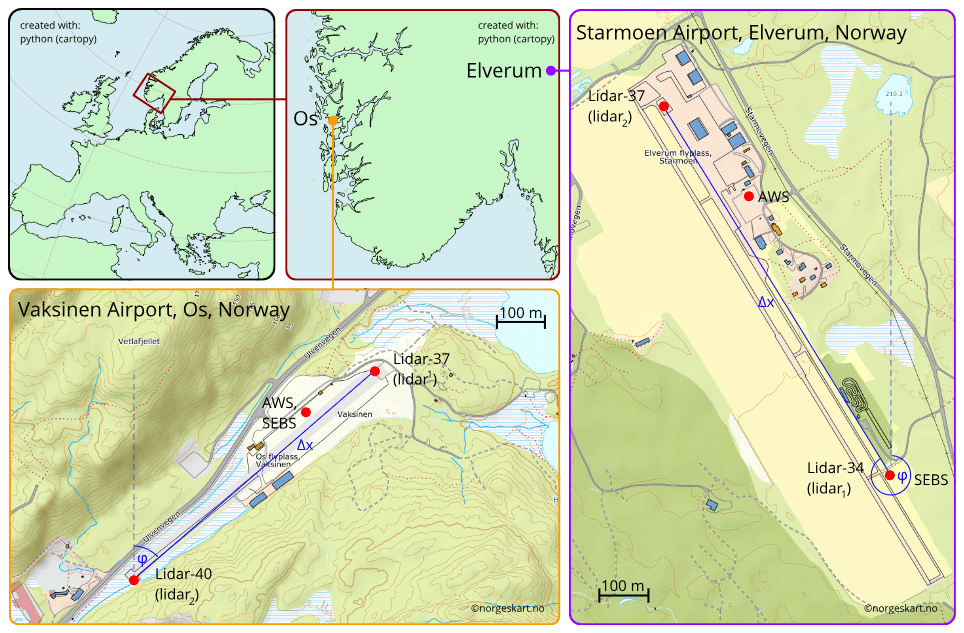
Figure 1 Location of the measurement sites and instrument setup. Top left: overview map of Europe. Top center: zoomed-in view of southern Norway with markers for the location of Os (orange) and Elverum (purple). Bottom left: overview of the measurement site at Vaksinen airport in Os with the locations of the utilized lidars, AWS, and SEBS indicated by red markers as well as distance, Δx, and angle, φ, relative to north between the lidars indicated in blue. Right: overview of the measurement site at Starmoen airport near Elverum with the locations of the utilized lidars, AWS, and SEBS indicated by red markers and Δx and φ indicated in blue.

2 The experiment

The data collected for this study originate from a similar experimental setup at two sites. The instrumentation installed at these two sites, the measurement strategy of the lidars, which are the main instrumentation of the setup, and the challenges, which were met during the experiment at each site, are introduced in the following sections.

2.1 The sites

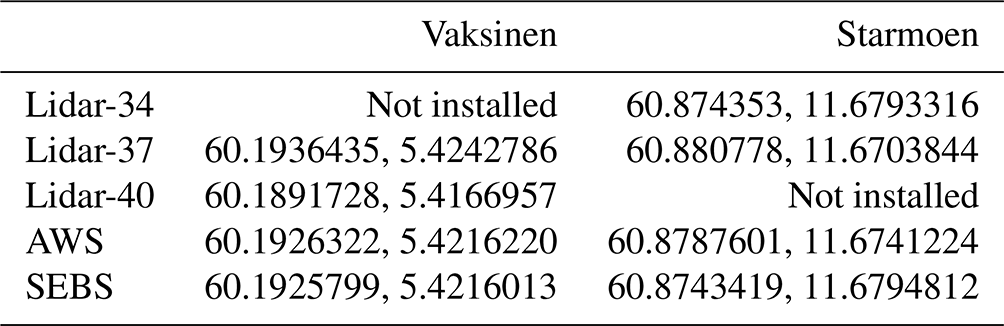
We have chosen two small airports in Norway for sailplanes and small motor planes as measurement sites for the dual-lidar experiment. From 12 May until 7 June 2021, we installed two WindCube-100S scanning lidars, an automatic weather station (AWS), and a surface energy balance station (SEBS) at Vaksinen airport, Os, in western Norway, ca. 25 km south of Bergen. The same instrumentation was deployed from 14 July until 30 July 2022 for the second field campaign at Starmoen airport, Elverum, in eastern Norway, about 120 km northeast of Oslo. Figure 1 shows the measurement sites and the location of the instrumentation, and Table 1 documents the coordinates of each instrument.

Table 1 Coordinates (^∘ N, ^∘ E) of the instrumentation at Vaksinen airport and Starmoen airport. The numbering of the lidars corresponds to the respective serial numbers of the WindCube-100S series.

2.2 The instrumentation

The AWS provides background information on the basic meteorological parameters of pressure, temperature, humidity, wind speed, wind direction, incoming shortwave radiation, and precipitation at 1 min temporal resolution. The SEBS measures the four components of the radiation balance, i.e., incoming and outgoing shortwave and longwave radiation, together with highly resolved (20 Hz) measurements of temperature, humidity, and three-dimensional wind speed, each variable at a single altitude above ground. In addition the SEBS also provided profile measurements of temperature, humidity and wind at 1, 2, and 4 m above the surface at a lower resolution (1 min). In this study, we utilize measurements from AWS and SEBS mainly to identify precipitation-free periods that favor convective conditions throughout the two campaigns and to estimate the surface heat flux (see Sect. 5.2) and flux Richardson number (see Sect. 5.3) as an indication of the presence of convection.

In both campaigns the two scanning lidars were installed with a relative distance, Δx (m), and angle, φ (^∘), relative to north to each other at opposing ends of the runway of the corresponding airfields (Fig. 1). The lidars observe radial velocity, v_r (m s⁻¹), which is the velocity of the wind projected to the line of sight (LOS) of the lidar beam. The scanning lidars used in the experiment can be programmed to point towards a direction corresponding to a certain azimuth angle, α (^∘), and an elevation angle, θ (^∘). For each combination of α and θ, v_r values are simultaneously obtained at several ranges, r (m), from the lidar.

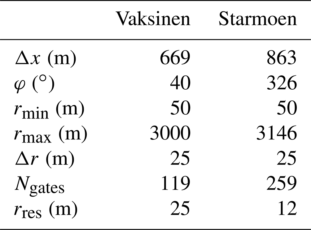
Along the lidar beam, each v_r value is observed as a composite of the Doppler velocity of all particles, which contribute to the lidar's backscattering signal (e.g., aerosols) within the lidar range gate length, Δr (m). The strength of the particle backscatter is related to the signal-to-noise ratio, SNR (dB), which is also recorded by the lidar. By default, the distance between the range gates, which defines the range gate resolution, r_res (m), is equal to Δr. Yet, r_res can also be set manually, e.g., smaller than Δr, such that range gates overlap. The minimum range, r_min (m), needs to be at least 2⋅Δr and the maximum range, r_max (m), is dependent on the number of utilized range gates, N_gates, and r_res. Table 2 summarizes the lidar parameter specifications utilized during the two campaigns.

Table 2 Dual-lidar setup specifications for the two sites at Vaksinen airport and Starmoen airport.

2.3 The lidar strategy

We utilized two lidar measurement strategies. In both campaigns, we sampled the three-dimensional wind profile using a Doppler beam swinging mode (DBS) with five consecutive beams: four beams, which are perpendicular at $\mathit{\alpha }=(\mathrm{0}{}^{\circ },\mathrm{90}{}^{\circ },\mathrm{180}{}^{\circ },\mathrm{270}{}^{\circ })$, each with θ=75^∘. The fifth beam points upward with θ=90^∘. The DBS is programmed to run for a duration, D_run, of 10 min within each hour. We retrieve an average of the wind profile over these 10 min, which we assume to be the representative profile for the corresponding hour.

The main strategy of the experiment aims to enable a retrieval of the plane-parallel horizontal and the vertical velocity components, u and w (m s⁻¹), in a vertical cross-section above the runway of each airport. As displayed in Fig. 2, this is achieved by range height indicator (RHI) scanning patterns performed by each lidar. Here, the lidar points horizontally to the complementing lidar (lidar₁: α=φ, lidar₂: $\mathit{\alpha }=\mathit{\phi }+\mathrm{180}$^∘, with θ=0^∘ orientation in the direction of φ) and then performs a continuous scan by changing θ (lidar₁: from θ=0 to 150^∘, lidar₂: θ=180 to 30^∘). The accuracy of the horizontal (azimuth) alignment was ensured by a hard-target calibration of each lidar at the start of the campaigns. We utilize a retrieval to estimate u and w from overlapping RHI scans of the two lidars in the vertical cross-section above the runway. The retrieval combines v_r values of the two lidars with different polar coordinate systems and achieves u and w values on a Cartesian grid (see Fig. 2). We document further details of this retrieval method and its shortcomings in Sect. 3.

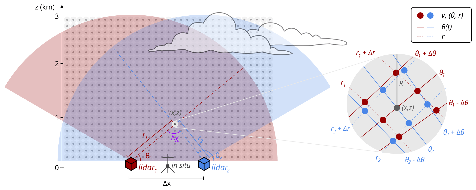
Figure 2 Vertical cross-section of the dual-lidar setup utilized during the campaigns at Vaksinen airport and Starmoen airport, respectively. The transparent red and blue surface areas represent the angular range covered by the RHI scans of the individual lidars, which are represented by the red and blue boxes. The dark grey dots represent a schematic of the Cartesian retrieval grid. A zoom in on to the polar grid of the two lidars and the corresponding positions of all v_r values used for the retrieval of u and w in an exemplary point (x,z) of the Cartesian grid is shown on the right-hand side of the figure.

Convection is a dynamic process, which may rapidly modify u and w on short timescales and small spatial scales. It is therefore an important goal of this study to investigate the combination of temporal and spatial RHI scan resolution that accurately captures the development of the convective circulation. The combination of the following parameters determines the temporal and spatial resolution of a single RHI scan. The scan speed, v_scan (^∘ s⁻¹), determines the duration, D_scan (s), of a single RHI scan, which spans a certain range of θ (i.e., 150^∘ from θ=30^∘ to θ=180^∘). The product of v_scan and the integration time, T_int (s), of the Doppler velocities that contribute to a single v_r values determines the angular resolution, Δθ (^∘), of the RHI scan.

High angular (spatial) resolution can be achieved with a low v_scan at the cost of a long D_scan and hence a low temporal resolution when keeping the angular range and T_int constant. On the other hand, by decreasing T_int, the angular resolution can be increased without changing v_scan and consequently without sacrificing temporal resolution for covering the same angular range in a scan. However, short T_int can result in poor quality of the measured data due to low SNR.

During the two campaigns, we tested different scanning configurations with varying balance between temporal and spatial resolutions, as well as integration time. These configurations are summarized in Table 3.

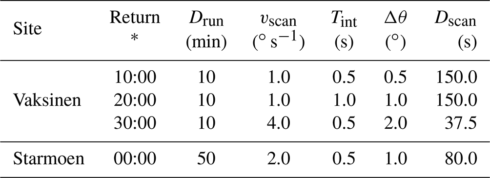
Table 3 Hourly returning schedule (^* starting each hour at MM:SS) of the RHI scan configurations during the Vaksinen and Starmoen campaign.

A major goal of the Vaksinen campaign was to evaluate the ability of different scan configurations to accurately map convection. At Vaksinen airport, several scanning patterns with either high temporal or high spatial resolution were run in sequence within a 1 h return period: first the wind profile was observed with a DBS scan for 10 min. Then the three scan configurations introduced in Table 3 were subsequently scheduled for 10 min each. This was followed by a series of fixed, out-of-plane RHI and plan position indicator (PPI) scans for 20 min. These latter scan configurations of the experiment are, however, not relevant for this study and thus not further described.

At Starmoen airport, we aimed to study the evolution of convection more continuously than during the Vaksinen airport campaign, utilizing longer D_run and sampling with only one scan configuration throughout the campaign (see Table 3). The RHI scan configuration is scheduled for 50 min, followed by a 10 min DBS scan. This schedule is repeated by each of the two lidars with a return period of 60 min throughout the campaign. The scan configuration chosen here is a compromise between the extremes of temporal or spatial resolution utilized during the Vaksinen campaign.

2.4 The challenges

During both campaigns, we encountered various challenges that affected the availability and quality of the data. At the Vaksinen airport site, there were several power outages that disordered the schedule of lidar-37 (northeastern end of Vaksinen airport, see Fig. 1), demanding a manual fix on site. This led to a substantial loss of data during several convective days, as the failure was first detected after a site visit. Also, the data download from the internal computer of the lidars was very slow, which delayed full recovery of the data, processing, and the identification of further problems occurring during the campaign until after the recovery of the instrumentation from the field. Despite the challenges encountered, we were able to secure representative observations from both lidars simultaneously during 1 very convective day (28 May 2021), which will be evaluated and discussed in Sect. 6.

As a consequence of the challenges during the Vaksinen airport campaign, we developed an upgraded version of our lidar setup. During the Starmoen campaign, the data were not only stored on the internal computer of the lidars, but also transferred via “sftp” protocol to a Raspberry Pi 4 Model B¹. The Raspberry Pi was integrated into a remote access system developed by the Geophysical Institute, University of Bergen, and solved the problem of the slow data download. The remote access system also includes an industrial router, which enabled real-time data upload and visualization of the lidar observations on a server provided by the Norwegian Research and Education Cloud (NREC²), as well as a time synchronization of the lidars independent from GPS. This enabled us to identify and already fix problems occurring during the campaign and ensured that the schedule of the lidar program was kept throughout the campaign. A future application of this remote access system includes, among others, remote control and programming of the lidar in the field.

Nonetheless, the period of installation at Starmoen airport was impacted by several precipitation events during the first half of the campaign, which almost completely depleted the aerosol content in the boundary layer. This strongly reduced the SNR obtained by the lidars and hence the reliability of the observed v_r. It required several convective days after the precipitation period for the SNR to increase such that sufficient data availability of v_r for processing and data analysis was achieved. After the precipitation period during the Starmoen campaign, mainly 1 convective day (29 July 2022) with weak synoptic wind and strong fluxes qualified for further detailed analysis (see Sect. 6).

3 Retrieval of the two-dimensional wind field

To retrieve the u and w wind components for any point (x,z) in the lidar cross-section at discrete points in time, we combine pre-processed v_r fields (see Sect. 4) from both lidars. The temporal resolution of the retrieved cross-sections is the same as the temporal resolution of the utilized v_r fields. As we save the v_r fields once per 1 s or even once per 0.5 s (see T_int in Table 3), we can retrieve u and w fields at any lower resolution that fits the purpose of interest. The methodology to estimate u and w from independent v_r observations and the errors connected to the method are documented in the two subsections below.

3.1 Retrieval principle

At any position (x,z) within the vertical cross-section of the overlapping RHI scans, v_r is related to the instantaneous u and w components of the real wind projected to the θ-dependent LOS of the lidar beam,

$$\begin{array}{}\text{(1)}& v_{\mathrm{r}}(x,z)=u(x,z)\cdot \cos \mathit{\theta }+w(x,z)\cdot \sin \mathit{\theta },\end{array}$$

with (x,z) connected to θ and r by

$$\begin{array}{}\text{(2)}& \left(\begin{array}{c}x\\ z\end{array}\right)=r\left(\begin{array}{c}\cos \mathit{\theta }\\ \sin \mathit{\theta }\end{array}\right)+\left(\begin{array}{c}{x}_{\mathrm{0}}\\ z_{\mathrm{0}}\end{array}\right),\end{array}$$

where x₀ and z₀ define the relative position of the lidar to the origin point (0,0) of the Cartesian coordinate system of choice for the retrieval. We set the location of the origin point at the individual ground level of the two sites in the middle of the two lidars.

To solve Eq. (1) for u and w in the point (x,z), we need to construct an equation system utilizing at least two observations of v_r, each obtained with an independent θ. Since lidars do not operate on a Cartesian coordinate system (x,z) but on individual polar coordinate systems (θ,r), there are very few combinations of θ and r for the two lidars for which the v_r observations fall into exactly the same point (x,z) in space (see Fig. 2). Still, retrieving the u and w on a Cartesian instead of a polar retrieval grid is a common approach to merge the observations of two lidars (e.g., Stawiarski et al., 2013; Adler et al., 2020; Haid et al., 2020).

Here, instead of using only two independent v_r observations in a single point (x,z), we construct an equation system (based on Eq. 1), containing all valid v_r values (excluding “not a number” or NaN values) and their individual dependencies on r and θ, from the two lidars within a radius, R, around the Cartesian point (x,z) of interest (see Fig. 2).

$$\begin{array}{}\text{(3)}& \left(\begin{array}{c}{v}_{r\mathrm{1}}(r_{\mathrm{1}},{\mathit{\theta }}_{\mathrm{1}})\\ v_{r\mathrm{2}}(r_{\mathrm{2}},{\mathit{\theta }}_{\mathrm{2}})\\ \cdot \\ \cdot \\ v_{rn}(r_n,{\mathit{\theta }}_n)\end{array}\right)=\left(\begin{array}{cc}\cos {\mathit{\theta }}_{\mathrm{1}}& \sin {\mathit{\theta }}_{\mathrm{1}}\\ \cos {\mathit{\theta }}_{\mathrm{2}}& \sin {\mathit{\theta }}_{\mathrm{2}}\\ \cdot & \cdot \\ \cdot & \cdot \\ \cos {\mathit{\theta }}_n& \sin {\mathit{\theta }}_n\end{array}\right)\left(\begin{array}{c}u\\ w\end{array}\right)\end{array}$$

The equation system can also be written in vector and matrix format.

$$\begin{array}{}\text{(4)}& {\mathit{v}}_{\mathrm{r}}=\mathbf{N}\mathit{v}\end{array}$$

If more than two independent v_r observations are within R to construct the equation system, it is over-constrained. To solve the over-constrained equation system which results from using R, we apply a least-squares approach (see Lai et al., 1978; Cherukuru et al., 2015) using matrix inversion:

$$\begin{array}{}\text{(5)}& \widehat{\mathit{v}}={\left({\mathbf{N}}^T\mathbf{N}\right)}^{-\mathrm{1}}{\mathbf{N}}^T{\mathit{v}}_{\mathrm{r}},\end{array}$$

where $\widehat{\mathit{v}}$ is the best fit of v considering all utilized v_r observations. Note that u and w are only retrieved if there is at least one valid v_r value provided by each lidar within R; otherwise, u and w are set to NaN in the corresponding Cartesian grid point.

It is also possible to incorporate v_r observations within a temporal radius, T_r, around the point of interest in time into the over-constrained equation system discussed above (see Newsom et al., 2008). Yet, the usage of T_r rather represents a temporal average of the flow field and is not meaningful when using instantaneous RHI scans which result from the temporal interpolation (see Sect. 4.2).

3.2 Retrieval errors and uncertainties

There are several sources of errors and uncertainties, which need to be considered for dual-lidar retrievals. Many errors in the single-lidar observation are projected and amplified in the co-planar, dual-lidar retrieval, e.g., lidar-specific uncorrelated noise and systematic error, as well as imprecise azimuth adjustment or leveling during the lidar setup and calibration (see, e.g., Stawiarski et al., 2013).

We attempt to minimize or avoid the errors and error amplifications that are connected to the dual-lidar retrieval. One prominent error in the dual-lidar retrieval is the temporal under-sampling error: the observations of v_r of the two lidars may each correspond to a different state of u and w due to a difference in the time at which v_r was observed by each lidar. Utilizing v_r values which do not correspond to the same state of u and w in reality will yield retrieved u and w values that may correspond to neither of the wind fields sampled by the individual lidar. The magnitude of the temporal under-sampling error is proportional to the absolute velocity difference in the flow field at the two time steps the two individual lidar obtained v_r (Stawiarski et al., 2013).

$$\begin{array}{}\text{(6)}& {\mathit{\sigma }}_{\mathrm{time}}\left(\mathrm{\Delta }t\right)\approx \left|v_{\mathrm{r}\mathrm{1}}\right(t_{\mathrm{1}})-v_{\mathrm{r}\mathrm{2}}(t_{\mathrm{2}}\left)\right|\end{array}$$

The time difference, $\mathrm{\Delta }t=|t_{\mathrm{2}}-t_{\mathrm{1}}|$, is dependent on the spatial location (x,z) in the dual-lidar cross-section. In Sect. 4.2 we introduce a processing procedure to minimize the temporal under-sampling error using instantaneous RHI cross-sections achieved from temporal interpolation instead of single scans. A further reduction of this error can be related to the usage of R and over-constrained equation systems to retrieve u and w for each point on the Cartesian grid. Here, temporal errors caused by small spatial displacement (within R) between two scans are averaged out.

For certain conditions the equation system (see Eq. 4) is ill-posed. In the case that the angles θ₁ and θ₂ of the two intersecting lidar beams are both close to horizontal or close to vertical, the v_r observations are not really independent. This is the case for $\mathrm{\Delta }\mathit{\chi }=|{\mathit{\theta }}_{\mathrm{1}}-{\mathit{\theta }}_{\mathrm{2}}|$, which is either very small or very large (see Fig. 2). When the two lidars are both pointing horizontally, the horizontal component dominates the v_r observations of both lidars and the retrieval error of w is amplified. In this case Δχ is either large (beams point towards each other) or small (both beam point in the same direction horizontally). Mainly vertically pointing beams result in small Δχ and will amplify the retrieval error of u. Yet, with a sufficiently large Δx, which is the case for our setups, the point at which the retrieval error of u becomes important is located above the retrieval grid. The amplification of the retrieval error, depending on Δχ, is defined by the factor σ_amp (see Stawiarski et al., 2013):

$$\begin{array}{}\text{(7)}& {\mathit{\sigma }}_{\mathrm{amp}}^i={\mathit{\sigma }}_{\mathrm{amp}}\cdot {\mathit{\sigma }}^i={\displaystyle \frac{\mathrm{1}}{{\sin }^{\mathrm{2}}\left(\mathrm{\Delta }\mathit{\chi }\right)}}\cdot {\mathit{\sigma }}^i,\end{array}$$

where σⁱ is a placeholder for any single- or dual-lidar error (e.g., the temporal under-sampling error). We remove all retrieved values of w that correspond to Δχ>150^∘ and Δχ<30^∘ to avoid strongly amplified single- and dual-lidar errors in the retrieval, such as those errors discussed in the paragraphs above.

Utilizing an over-constrained equation system enables quantifying the uncertainty in the retrieved wind field. The least-squares retrieval yields the best fit and hence a single retrieved value $\widehat{u}$ or $\widehat{w}$. By projecting these retrieved $\widehat{u}$ and $\widehat{w}$ values back onto the LOS (see Eq. 1), which yields a single value $v_{\mathrm{r}}(\widehat{u},\widehat{w})$ for each grid point (x,z), we can estimate the root mean square error, RMSE (m s⁻¹).

$$\begin{array}{}\text{(8)}& \text{RMSE}=\sqrt{{\displaystyle \frac{\mathrm{1}}{N}}\sum _{n=\mathrm{1}}^N{\left|v_{\mathrm{r}}\left({\mathit{\theta }}_n,r_n\right)-v_{\mathrm{r}}\left(\widehat{u},\widehat{v}\right)\right|}^{\mathrm{2}}}\end{array}$$

The RMSE is estimated on the basis of all N points of v_r within each R. This metric is useful to identify regions where processes are averaged over the area covered by R on the discrete Cartesian retrieval grid or where the temporal interpolation (Sect. 4.2) is not able to accurately restore the dynamic behavior of the convective circulation.

4 Processing of dual-scanning lidar observations

Before combining the v_r values from the two lidars into the u and w wind components, the RHI scan data from individual instruments require processing. In particular, the data need to be filtered for noise and erroneous features. After filtering, we apply temporal gap filling using interpolation by replacing discarded data points, and achieve instantaneous RHI scans with an increased temporal resolution.

4.1 Radial velocity filtering

We apply v_r data filtering to all utilized lidar scanning patterns (RHI and DBS). In a first step, we remove all v_r observations with absolute values exceeding 30 m s⁻¹, as they are unrealistically high for convective conditions. Further, we have observed three types of problems with the data: individual data points with noise; larger irregular “streak” patterns in the RHI scans, which can be associated with range-folded ambiguities as described by Bonin and Brewer (2017); and irregular patterns, which result from interaction with obstacles. For the retrieval (Sect. 3) to work, it is critical to remove the areas with points that correspond to these erroneous features and large spatial patches of noise. We address these problems by using the Density-Based Spatial Clustering of Applications with Noise (DBSCAN) algorithm, which was previously used by Alcayaga (2020) to filter PPI scans of Doppler lidar observations. In contrast to conventional filters, this clustering algorithm does not apply a fixed threshold to either SNR or v_r. Instead, the DBSCAN algorithm detects clusters of dense data points characterized by both v_r and SNR. Therefore, it can distinguish between reasonable v_r observations and noise in the same SNR range. This allows for the recovery of reliable v_r values for SNR values even below −30 dB, which would be lost if the SNR threshold of −27 dB that is suggested by the lidar manufacturer (Leosphere) were applied.

We use the implementation of the DBSCAN algorithm in the “scipy” Python package (Virtanen et al., 2020) to identify clusters of data points in the SNR–v_r space. Figure 3 displays the application of the DBSCAN filter for one example RHI scan obtained during the Starmoen campaign on 29 July 2022 starting at 14:20 UTC.

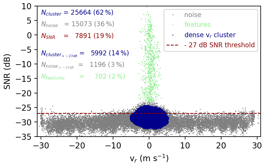
Figure 3 Scatter of v_r against SNR, with a DBSCAN-identified cluster of dense scatterers (valid v_r) marked in blue, rarefied scatterers (noise) marked in grey, and rarefied scatterers corresponding to features marked in mint. The number of points (and the percentage relative to all data) classified as noise (N_noise, grey), features (N_features, mint), and clusters of reasonable points (N_cluster, blue) are documented in the upper left corner. The dashed red line indicates the −27 dB SNR threshold. Values of v_r corresponding to SNR values below this line are discarded by the SNR filter. N_SNR (red) corresponds to the number of points (and percentage relative to all data) recovered by the SNR filter, while $N_{{\mathrm{cluster}}_{>-\mathrm{27}\mathrm{dB}}}$ (blue) and $N_{{\mathrm{noise}}_{>-\mathrm{27}\mathrm{dB}}}$ (grey) correspond to the number of scatterers (and percentage relative to all data) recovered by the SNR filter but attributed to the points corresponding to noise and reasonable values by the DBSCAN filter, respectively.

Here, v_r is scattered against SNR and data points which are identified as reasonable by the DBSCAN filter (dense scatterers) are highlighted in blue, while data points identified as noise (rarefied scatterers) are displayed in grey. In addition, we highlighted scatterers in mint that correspond to features in the scan, though it should be noted that here these features fall into the same rarefied DBSCAN cluster as the noise.

The DBSCAN algorithm clusters scatterers as dense (cluster) or non-dense (noise) depending on a density radius, ϵ, and minimum number of samples, n_sample. Our criterion for choosing a combination of ϵ and n_sample was, apart from the noise, that only one main cluster was identified and any secondary cluster needed to be separated from that main cluster by at least 3ϵ. The same ϵ and n_sample need to fulfill this criterion for all scans of the same sample size and hence for all scans using the same scan configuration. To determine the parameters for each scan configuration, we kept ϵ constant and adjusted n_sample according to the change in absolute sample size. For RHI scans the DBSCAN algorithm with corresponding ϵ and n_sample was applied to each cross-section individually, while for the DBS scans, the DBSCAN algorithm was applied to the 10 min time series of each beam direction individually. Specific to the number of points sampled in the RHI scan presented here, we apply ϵ=0.6 and n_sample=150.

For the example displayed in Fig. 3, the DBSCAN algorithm identifies a cluster of v_r values as reasonable, which makes up 62 % of the observed data points. The remaining 38 % of the data points are classified as noise (36 %) or features (2 %), such as range-folded ambiguities (Bonin and Brewer, 2017), obstacles, and clouds. The majority of noise identified by the DBSCAN algorithm (31 %) is evident just below SNR $=-\mathrm{27}$ dB, where v_r fluctuates ±30 m s⁻¹. In order to remove noise from the v_r data the conventional SNR threshold is therefore reasonably set to −27 dB. However, when applying the SNR threshold filter to the RHI scan, only 19 % of the v_r values are kept and a large amount of data identified as reasonable by the DBSCAN filter (48 %) are discarded. Further, only 14 % of the data points are both above the SNR threshold and within the cluster identified as reasonable by the DBSCAN algorithm, while 5 % of the data points which are above the SNR threshold are classified as noise (3 %) or irregular erroneous features and clouds (2 %).

Figure 4 shows the RHI cross-sections of v_r values (Fig. 4a) and SNR values (Fig. 4b) that are scattered against each other in Fig. 3, as well as the filtered v_r values using the SNR threshold (Fig. 4c) and using the DBSCAN algorithm (Fig. 4d). This depiction allows us to investigate the ability of the SNR threshold filter as well as the DBSCAN filter to discard noise and erroneous features, while retaining valid data points. The situation captured on 29 July 2022 at Starmoen by this RHI scan is convective and rather complex, which is evident mainly from the convergence of the horizontal velocity close to the surface around the $x=-\mathrm{1}$ km horizontal of distance mark, visible in the non-filtered v_r data (Fig. 4a). The obtained SNR is very low (below −27 dB) both close to lidar and at a larger range (Fig. 4b). For r beyond ≈ 2 km distance from the lidar the originally observed v_r values (Fig. 4a) are irregular and noisy, while they appear rather regular close to the lidar despite the comparable low SNR (Fig. 4b). Only for r between 0.8 and 1.8 km from the lidar is the SNR increased overall. Additionally, several features of partially irregular v_r values, which correspond to local, strongly increased SNR, are visible (Fig. 4b). We identify range-folded ambiguities around $(x,z)=(\mathrm{1.0},\mathrm{0.5})$ and $(x,z)=(-\mathrm{3.0},\mathrm{0.5})$ km, a physical obstacle which blocks the LOS around $(x,z)=(-\mathrm{1.2},\mathrm{0.0})$ km, and a cloud around $(x,z)=(-\mathrm{2.0},\mathrm{2.3})$ km. These features are also apparent in the v_r values (Fig. 4a) and highlighted in mint in the RHI cross-section with the DBSCAN filter applied (Fig. 4d).

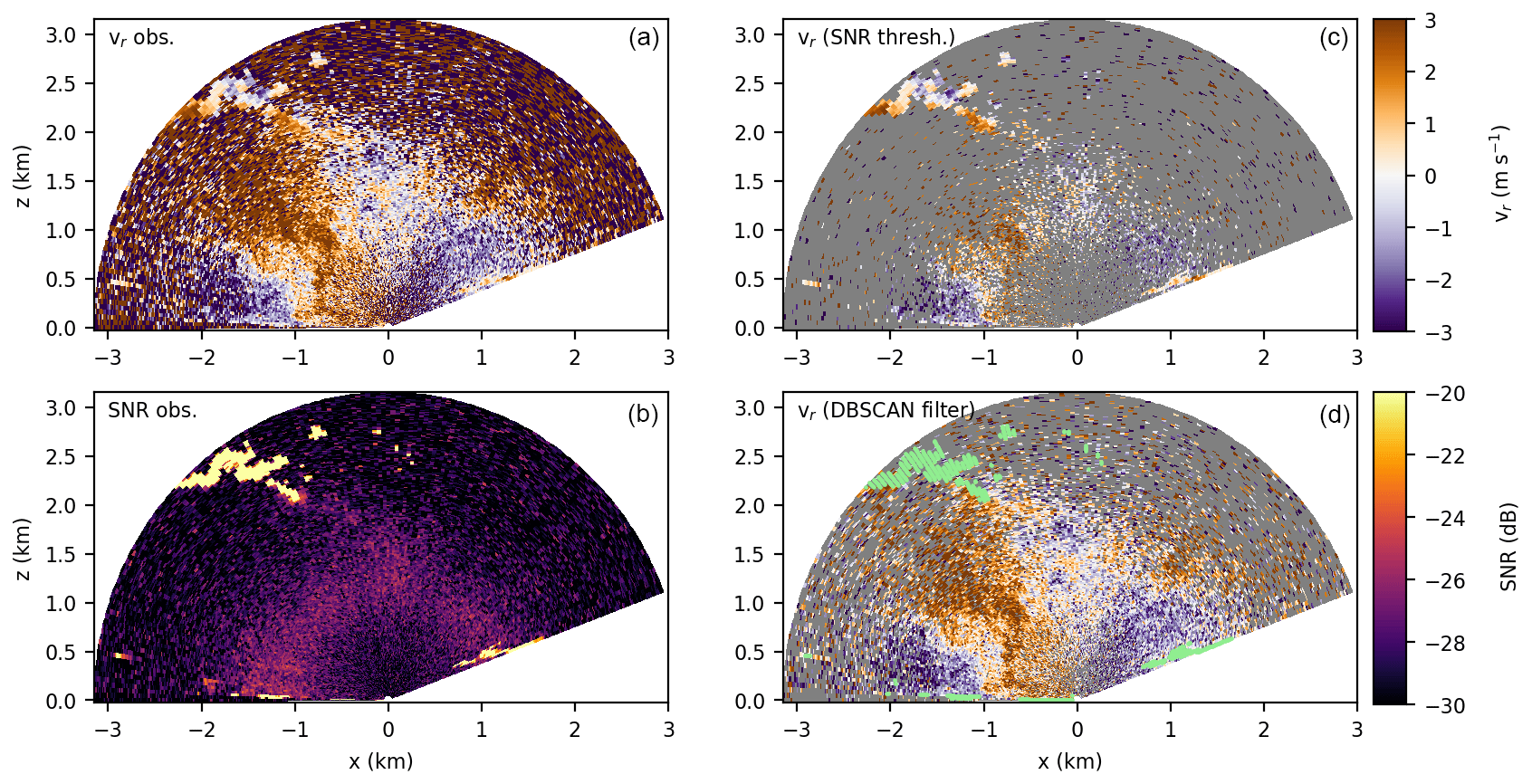
Figure 4 Sample RHI scan from the Starmoen campaign on 29 July 2022 at 14:20 UTC with (a) observed v_r, (b) observed SNR, (c) filtered v_r using an SNR threshold, and (d) filtered v_r using the DBSCAN clustering algorithm. Grey areas correspond to filtered values flagged as NaN by the (c) SNR threshold filter or the (d) DBSCAN filter. Features also flagged as NaN by the DBSCAN filter are highlighted in mint.

The SNR threshold filter (Fig. 4c) removes a large number of v_r values within a 1 km radius around the lidar and at r larger than 2 km from the lidar. Yet, erroneous v_r values corresponding to range-folded ambiguities are not filtered out. On the basis of the remaining v_r data, the convective circulation is hardly recognizable. The RHI scan observed during the same time period from the complementary lidar experiences a similar extreme reduction of v_r values when applying the SNR threshold filter (not shown here). As a consequence the region of valid overlapping v_r is even more reduced and will yield an even less valuable retrieval of u and w after applying the SNR threshold filter.

The DBSCAN filter (Fig. 4d), on the other hand, successfully removes noise, which is clearly evident in the non-filtered v_r observations (Fig. 4a) at r>2 km from the lidar. Reasonable v_r values with SNR $<-\mathrm{27}$ dB, which follow the same radial velocity patterns as the surrounding non-noisy points that are above the −27 dB threshold, are not filtered close to the lidar or at larger distances. In contrast to the SNR threshold filter (Fig. 4c) the information about the convective flow field is retained by the DBSCAN filter (Fig. 4d). The small number of points attributed to noise above −27 dB by the DBSCAN algorithm (3 %) are distributed over the cross-section and therefore have no relevance for the retrieval performance. Here, a sufficient number of valid v_r values are within R for most Cartesian points covering the convective circulation. Further, most range-folded ambiguities and features caused by blocking of LOS by obstacles are removed from the data. Unfortunately, this also includes parts of the data points obtained within clouds, which is of interest for the convective circulation. Still, the gain of retained data points corresponding to the convective circulation (48 %) within the boundary layer outweighs the loss of data points within the cloud (<2 %) at the edge of the circulation achieved by the DBSCAN filter.

The example presented in Figs. 3 and 4 corresponds to conditions with comparably low aerosol content due to preceding periods with precipitation during the Starmoen campaign. Considering the composite of relevant RHI scans throughout the convective day at Starmoen (29 July 2022) which is presented in this study, the DBSCAN filter discards 61 % (and retains 39 %) of data points, while the SNR filter discards 85 % (and retains only 15 %) of data points. The lower recovery rates compared to the presented example are mainly due to lower boundary layer depths at earlier hours during the day (see Sects. 5.1 and 6.1). During the Vaksinen campaign, we did not sample any precipitation event in the period prior to the convective day, which is presented as an example case in this study. As a consequence, aerosols could accumulate in the boundary layer, and SNR was comparably high. Filtering by DBSCAN (discarded: 38 %, retained: 62 %) and SNR threshold (discarded: 60 %, retained: 40 %) yielded comparably lower rates of removal for the evaluated convective day at Vaksinen (28 May 2021). Even lower and more similar removal rates are found for the DBSCAN filter (discarded: 19 %, retained: 81 %) and the SNR threshold filter (discarded: 23 %, retained: 77 %) on 28 May 2021 when considering only the filtered values within the boundary layer (for boundary layer depth estimation see Sect. 5.1). Here, the DBSCAN filter outperforms the SNR threshold filter, mainly by removing noise and range-folded ambiguities which are also present at SNR $>-\mathrm{27}$ dB.

Due to the improved data quality and availability, we prepare the v_r data for further processing by applying the DBSCAN filter to each RHI scan (and DBS scan series) throughout the evaluated convective days of both campaigns. Since the DBSCAN algorithm is relatively costly in terms of computational power, we store the filtered data in hourly NetCDF files, along with the other relevant variables observed by the lidar. This dataset is utilized in the following processing step.

4.2 Temporal interpolation

Dependent on the scan configuration (Table 3), each individual RHI scan takes a few tens of seconds up to 2.5 min. Consequently, the RHI scans used for the reconstruction of the wind field between the two lidars are not instantaneous snapshots of the radial velocity field. Only the observations along the beam of a single θ correspond to the same time step within the same RHI scan. Even if the RHI scans of the two lidars are perfectly synchronized, only a very small number of spatially overlapping points in the cross-section (see Fig. 2 and Röhner and Träumner, 2013) are observed without any time lag between the two lidars. For any fixed point in the overlap of the lidar scans, the maximum possible time difference between observations by each lidar is bound by D_scan. If the time difference is considerably large, the convective wind field observed as v_r at a certain point in the cross-section by one lidar can strongly differ from the wind field observed by the complementing lidar. Such temporal deviation of the v_r observations in a given point propagates and is amplified as a temporal under-sampling error in the retrieval of u and w (see Sect. 3.2).

To reduce the impact of the temporally induced error, we test the usage of an instantaneous lidar cross-section, achieved by temporal interpolation. For that, we interpolate linearly between each $v_{\mathrm{r}}(r,\mathit{\theta },t)$ and $v_{\mathrm{r}}(r,\mathit{\theta },t+D_{\mathrm{scan}})$, located in the same position in space (r,θ) yet at the time of the next scan (t+D_scan). The highest time resolution of the interpolated grid corresponds to one RHI cross-section every T_scan of the respective scan configuration (see Table 3). From an interpolated array of v_r values (with three dimensions: θ, r, t) we can now extract instantaneous cross-sections, where all v_r values correspond to one specific time stamp. Only values corresponding to one single θ are actually observed by the lidar in this scan, and the remaining values are a result of the interpolation. A big advantage of the temporal interpolation is that we can utilize cross-sections from the two lidars that correspond to the exact same t. Hence, when using temporal interpolation, perfect synchronization of the RHI scans of the two lidars is not required. The v_r values will still be most accurate around the θ that is observed at the time step to which the instantaneous scan is interpolated. Synchronization of the lidar scans mainly achieves a line of no time lag located along the vertical profile above the mid-point between the two lidars. Yet, convective eddies are not necessarily located directly in the middle of the lidars.

To demonstrate how the maximum possible error of the interpolated scan compares to the maximum possible error between non-interpolated, consecutive scans, we create an interpolated series. To achieve this, we interpolate between every second RHI scan obtained. Here, we actually create two interpolated series based on both the odd and even RHI scans to double the number of interpolated cross-sections. From both of these interpolated series we extract the v_r values that correspond to θ(t) of the RHI scans, which are not used to create an interpolated series. Thus, we can estimate the average difference between an interpolated and the control RHI scan to quantify the error in the interpolated series, e_int. It should be mentioned that e_int is conservative, as the real interpolation is performed for only the half-time-step of the presented validation method. Also, in contrast to an instantaneous cross-section, here all extracted v_r values from the interpolated series correspond to the maximum time lag within the cross-section, which is D_scan.

In a next step, we want to investigate the difference of e_int compared to the conservative temporal under-sampling error of the corresponding RHI scan series. We expect the maximum temporal under-sampling error for points where v_r values are measured with the maximum possible time lag of D_scan between the data points of two synchronized RHI scans. The average difference between two consecutive scans therefore gives an estimate of the maximum expected temporal under-sampling error, e_con, of the RHI scan series. In addition to e_con, we also estimate the temporal under-sampling error, merged for odd and evenly skipped RHI scan series, e_skip, which is the RHI scan resolution ($\sim \mathrm{2}\cdot D_{\mathrm{scan}}$) we used to estimate the interpolated series on which e_int is based. Figure 5 shows time series of these three error estimates e_skip, e_con, and e_int, how much e_int decreases in comparison to e_con, and how both of these error estimates behave in comparison to e_skip for two cases at the Starmoen and the Vaksinen site. We only consider values of the RHI scans which are within the boundary layer and hence below the boundary layer depth; see Sect. 5.1.

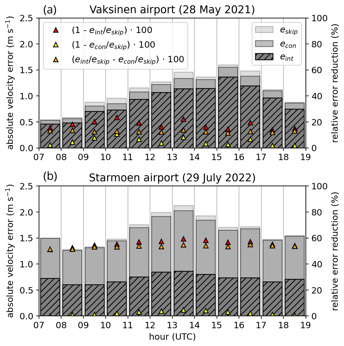
Figure 5 Maximum estimates of the temporal under-sampling errors for consecutive RHI scans (e_con) and for every second RHI scan (e_skip) as well as the temporal interpolation error (e_int) at (a) the Vaksinen site on 28 May 2021 between 07:00 and 19:00 UTC and at (b) the Starmoen site on 29 July 2022 between 07:00 and 19:00 UTC. For both sites, the error reduction of e_con and e_int relative to the largest expected error e_skip is also displayed with triangles on a secondary right-bound y axis.

For the case on 28 May 2021 at the Vaksinen site (Fig. 5), the error estimates correspond to the scan configuration with the highest temporal scan resolution (D_scan=37.5 s). Unfortunately, the other two scan configurations (see Table 3) utilized during the Vaksinen campaign do not provide a sufficient number of RHI scans to estimate a representative estimate of e_int.

With enhanced convective activity during the daytime hours, all three error estimates on 28 May 2021 (Fig. 5a) generally increase from 07:00 until 16:00 UTC. Within the early hours of the day (07:00–09:00 UTC), the average total error between consecutive scans is low (∼ 0.5 m s⁻¹) and increases to ∼ 1.5 m s⁻¹ at the peak of the convective activity (15:00–16:00 UTC). Over the course of the day, e_con improves by 2 %–10 % compared to e_skip, while e_int is consistently reduced by at least 10 % and up to 25 % compared to e_skip. The improvement of e_skip is approximately ∼ 15 % larger when using interpolation instead of a doubled time resolution throughout almost the whole convective day.

In comparison to the temporal error series displayed for the Vaksinen site (Fig. 5a), each RHI scan utilized to estimate the temporal error at the Starmoen site (Fig. 5b) takes approximately twice as long to complete (D_scan=80 s). Overall, temporal under-sampling errors estimated for the convective day at Starmoen (Fig. 5b) are larger than at Vaksinen (Fig. 5a). Also, all error estimates sampled on 29 July 2023 (Fig. 5b) reach their peak about 2 h earlier (between 13:00 and 14:00 UTC), exceeding 2 m s⁻¹. Here, error reduction by simply doubling the temporal resolution of the RHI scans is negligible (≤5 %). Strikingly, temporal interpolation strongly reduces the temporal under-sampling errors. For each displayed hour, e_int corresponds to less than half of the amount estimated for e_skip and e_con.

The much stronger error reduction by temporal interpolation for the Starmoen compared to the Vaksinen case can be partially linked to the longer (D_run=50 min) and hence more continuous RHI series at Starmoen. The representation of individual convective structure dynamics potentially also benefits more from temporal interpolation for the Starmoen than for the Vaksinen case. Given that in both evaluated cases (Fig. 5a and b) the interpolation consistently reduces the temporal under-sampling errors (e_skip and e_con) and that it has a larger improving effect than simply increasing (here doubling) the time resolution, we utilize interpolated instantaneous RHI scan series for all further processing steps.

5 Convective boundary layer parameters

In addition to the retrieval of the two-dimensional velocity field $(\widehat{u},\widehat{w})$, we estimate several boundary layer parameters based on complementary measurements from the lidars, the SEBS, and the AWS, but also from further processing the retrieved velocity field.

5.1 Boundary layer depth

We estimate the boundary layer depth on the basis of the derivative of unprocessed SNR with altitude. For both campaigns, the lidars are scheduled to obtain mainly RHI cross-sections. With Eq. (2) we can estimate the z coordinate corresponding to each SNR(θ,r) value and collapse all SNR values of a RHI cross-section to a single profile. We further average the profile for altitude bins of 25 m. For the boundary layer depth estimate, we distinguish between clear-sky and cloud-topped boundary layers.

For clear sky, relatively increased SNR values are usually connected to an increased number of aerosol particles in the air. Convection usually enhances the transport of aerosols (Kunkel et al., 1977), and hence aerosol particles are usually more numerous in the convective boundary layer than in the free atmosphere aloft. Hence, at the border between the boundary layer and free atmosphere, a strong decrease in SNR is usually observed. The height at which we identify the strongest decrease in SNR with height is therefore estimated to be the “clear-sky” or “dry” boundary layer height (m a.s.l.). We define the clear-sky boundary layer depth as the distance between the surface and the clear-sky boundary layer height.

For atmospheric conditions in which convective clouds form, we expect the SNR to rapidly increase at the cloud base, as cloud droplets reflect the lidar beam even more strongly than aerosol particles. Usually the lidar beam is absorbed after it penetrates a few range gates into the cloud and SNR strongly decreases again. During convective conditions with clouds, we assume the convective cloud-base height to be the upper limit of the boundary layer. We identify the cloud-base height at the altitude, where SNR increases the most strongly with height. We define the cloud-topped boundary layer depth as the distance from the surface to the cloud-base height.

5.2 Turbulent surface heat fluxes

The eddy covariance instrumentation of the SEBS, utilized in both campaigns, provides measurements of the three-dimensional wind vector, $(u,v,w)$ (m s⁻¹), the sonic temperature, T_s (^∘C), and the specific humidity, q (kg kg⁻¹), at 20 Hz time resolution. From the time series of w, T_s, and q, we extract the fluctuations w^′, $T_{\mathrm{s}}^{\prime }$, and q^′ by removing the 30 min average from the measured time series. Then we estimate the 30 min averaged sensible heat flux, H_s (based on Stull, 1988):

$$\begin{array}{}\text{(9)}& H_{\mathrm{s}}={\mathit{\rho }}_{\mathrm{air}}\cdot c_p\cdot \stackrel{\mathrm{‾}}{w^{\prime }{T}_{\mathrm{s}}^{\prime }},\end{array}$$

with the heat capacity of air c_p=1003.5 J kg⁻¹ K⁻¹ and the covariance of w^′ and $T_{\mathrm{s}}^{\prime }$ averaged over a 30 min interval. We further estimate the 30 min averaged latent heat flux, H_e (based on Stull, 1988):

$$\begin{array}{}\text{(10)}& H_{\mathrm{e}}={\mathit{\rho }}_{\mathrm{air}}{L}_v\cdot \stackrel{\mathrm{‾}}{w^{\prime }{q}^{\prime }},\end{array}$$

with the density of air, ρ_air≈1.25 kg m⁻³, and the latent heat of water, $L_{\mathrm{v}}=\mathrm{2264.705}\times {\mathrm{10}}^{\mathrm{3}}$ J kg⁻¹. The covariance of w^′ and q^′ is also averaged over the 30 min interval.

5.3 Flux Richardson number

In the unstably stratified boundary layer, the source of turbulence generation is either buoyancy or shear. The dimensionless ratio of these two terms is defined as the Richardson number. With our setup, the assumption of horizontal homogeneity, and neglecting subsidence, we can estimate the near-surface flux Richardson number, Ri_f (based on Stull, 1988):

$$\begin{array}{}\text{(11)}& {\mathit{Ri}}_{\mathrm{f}}={\displaystyle \frac{-\frac{g}{\stackrel{\mathrm{‾}}{\mathit{\theta }}}\cdot \stackrel{\mathrm{‾}}{w^{\prime }{T}_{\mathrm{s}}^{\prime }}}{\left|\stackrel{\mathrm{‾}}{u^{\prime }{w}^{\prime }}\frac{\mathrm{\Delta }\stackrel{\mathrm{‾}}{u}}{\mathrm{\Delta }z}\right|+\left|\stackrel{\mathrm{‾}}{v^{\prime }{w}^{\prime }}\frac{\mathrm{\Delta }\stackrel{\mathrm{‾}}{v}}{\mathrm{\Delta }z}\right|}},\end{array}$$

where g=9.81 m s⁻¹ is the Earth's gravitational acceleration constant and $T_{\mathrm{s}}^{\prime }$, u^′, v^′, and w^′ are fluctuations relative to the 30 min average values $\stackrel{\mathrm{‾}}{u}$, $\stackrel{\mathrm{‾}}{v}$, $\stackrel{\mathrm{‾}}{w}$, and $\stackrel{\mathrm{‾}}{T_{\mathrm{s}}}$ of the series measured by the SEBS. The sonic anemometer was installed 3 m above the surface and $\stackrel{\mathrm{‾}}{\mathit{\theta }}$ was estimated on the basis of $\stackrel{\mathrm{‾}}{T_{\mathrm{s}}}$ utilizing the pressure, p (hPa), measured by the AWS. The 30 min average vertical gradients, $\frac{\mathrm{\Delta }\stackrel{\mathrm{‾}}{u}}{\mathrm{\Delta }z}$ and $\frac{\mathrm{\Delta }\stackrel{\mathrm{‾}}{v}}{\mathrm{\Delta }z}$, are estimated from the profile measurements of $\stackrel{\mathrm{‾}}{u}$ and $\stackrel{\mathrm{‾}}{v}$ (gradient between cup anemometers and wind vanes installed at 2 and 4 m).

Only for negative Ri_f is turbulence generated by buoyancy, while for positive Ri_f buoyancy suppresses turbulence. For ${\mathit{Ri}}_{\mathrm{f}}\approx -\mathrm{1}$, production of turbulence is balanced between buoyancy and shear, while buoyancy dominates the turbulence generation for ${\mathit{Ri}}_{\mathrm{f}}<-\mathrm{1}$.

5.4 Convective updraft location

Buoyancy is also the generating mechanism for the convective circulation, which represents the largest eddies in the boundary layer. Convective (buoyant) motion is initiated due to horizontal density anomalies (see Jeevanjee and Romps, 2015). Locally reduced density at the surface (e.g., by a local temperature increase) results in upward motion of air (buoyant updraft), which is compensated for by a horizontal flow towards the updraft region (horizontal convergence). Consequently, we can utilize the retrieved velocity fields of u(x,z) and w(x,z) to identify the presence and the location, x_up, of a convective updraft. Generally two conditions need to be met within the lowest hundreds of meters for the presence of a convective updraft at x_up: a sufficient updraft velocity w(x)>0.5 m s⁻¹ and a negative horizontal divergence $\frac{\mathrm{\Delta }u}{\mathrm{\Delta }x}\left(x\right)<\mathrm{0}$ s⁻¹. As an additional condition, turbulence generation should not be suppressed by buoyancy (Ri_f<0) during the corresponding time.

6 Two convective case studies

We demonstrate the potential of dual-lidar observations and retrieval for studying convection on the basis of data collected during two convective days. Each day corresponds to one of the campaigns at Vaksinen and Starmoen airport. The cases represent a variety of scan configurations, surrounding terrain, and meteorological conditions. Considering the challenges during the two campaigns (see Sect. 2.4), the two days of choice (28 May 2021 and 29 July 2022) provide the most robust observations, namely those with the most favorable convective conditions and highest data availability during each of the campaigns. It should be noted that these two examples are a proof of concept for the potential of the dual-lidar approach to study convection. A generalization of the presented findings for a wide range of convective conditions will require longer observational periods.

6.1 Meteorological conditions and energy balance

Though obtained in May 2021 and July 2022 at different locations, the incoming shortwave radiation, SW_↓ (W m⁻²), is of similar magnitude for both evaluated days (clear sky: SW${}_{\downarrow ,max}\approx \mathrm{750}$ W m⁻², shown in Fig. 6). Both cases show a diurnal cycle in temperature, humidity, and wind, which is slightly lagged with respect to the SW_↓ series. Compared to the case shown for the Vaksinen site, the near-surface wind is slightly weaker and the diurnal temperature amplitude is larger at the Starmoen site. As a consequence, the turbulence generation during hours of net radiative forcing is mainly buoyancy-dominated (${\mathit{Ri}}_{\mathrm{f}}<-\mathrm{1}$) at Starmoen, while at Vaksinen turbulence generation is rather balanced between buoyancy and shear (${\mathit{Ri}}_{\mathrm{f}}\approx -\mathrm{1}$). Despite the different forcing mechanisms for turbulence generation, the sensible and latent turbulent surface heat fluxes are of comparable magnitude for both cases displayed in Fig. 6.

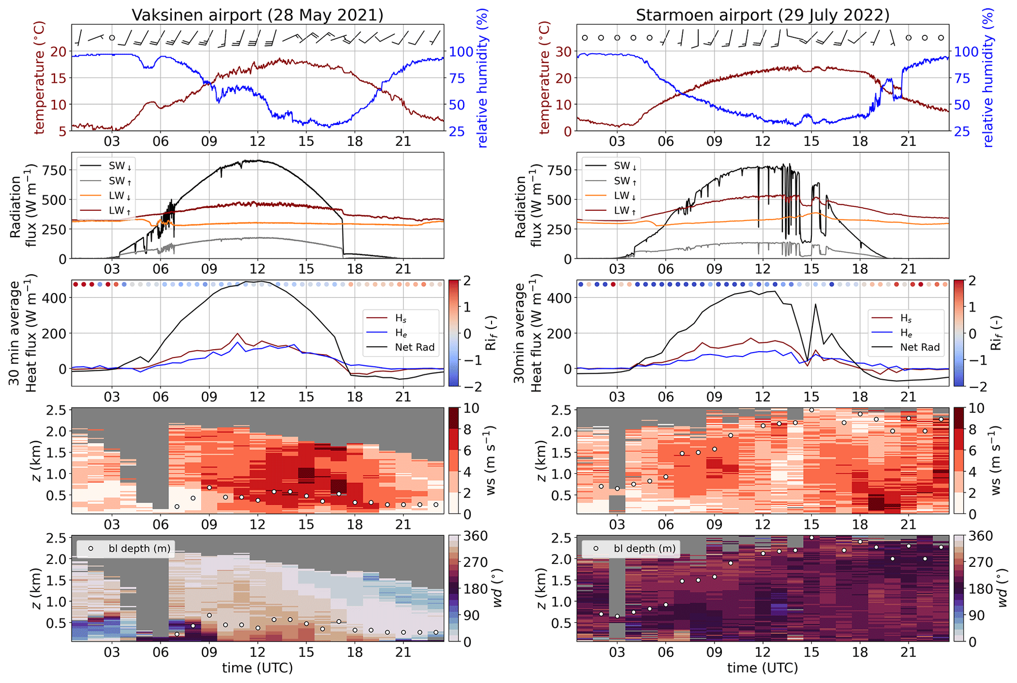
Figure 6 Diurnal cycle of temperature, humidity, and surface wind barbs (short feathers: 1 m s⁻¹, long feathers: 2 m s⁻¹) measured by AWS, incoming (↓) and outgoing (↑) longwave (LW) and shortwave (SW) radiation, net radiation, turbulent sensible (H_s) and latent heat (H_e) fluxes measured and estimated from SEBS measurements, temporal evolution of wind speed (ws) and wind direction (wd) profiles, and boundary layer depth (bl depth; m above the surface) from lidar observations during two convective days. Left panels: observations at Vaksinen airport (28 May 2021); right panels: observations at Starmoen airport (29 July 2022).

Throughout both days, we observe a net radiative forcing of up to 490 W m⁻² at the Vaksinen site and up to 460 W m⁻² at the Starmoen site (see Fig. 6). The latent and sensible heat fluxes make up ca. 55 % and ca. 60 % of the net radiation forcing at the Vaksinen and the Starmoen site, respectively. A maximum residuum of ca. 225 W m⁻² at Vaksinen and 180 W m⁻² at Starmoen remains around the period of peak net radiative forcing. The main part of this residuum is usually compensated for by the ground heat flux (not measured here), which can reach values of the order of a few hundred Watts per square meter (W m⁻²) (e.g., Arya, 2001). Still, large convective eddies, which are nearly stationary over the averaging period of the turbulent flux (30 min), may contribute substantially to the energy transport away from the surface. The contribution of such large eddies is not necessarily captured by the turbulent surface heat fluxes. With the dual-lidar setup, on the other hand, we can get a qualitative estimate of the larger-scale flow patterns and their evolution.

The wind speed and direction profiles reconstructed from the DBS scans and the boundary layer depth estimated from SNR profiles based on composites of all RHI scans already give a good overview of the predominating state of the circulation over the two chosen days (Fig. 6, two lower rows). Similar to the surface wind, wind speed is also increased throughout the whole profile at the Vaksinen site compared to the Starmoen site, in particular during the convective hours of the day (Fig. 6). Wind direction changes substantially both in time and with altitude at the Vaksinen site, turning from southerly to southwesterly (almost parallel to the airstrip) in the boundary layer during the convectively active hours. Above the boundary layer, wind direction turns towards north and later on towards east. At Starmoen, wind is mostly from south to southwesterly directions over the whole day and observed altitude range, which is almost perpendicular to the airstrip. The most striking difference between the two cases is the large difference in boundary layer depth. At the Vaksinen site the boundary layer is quite shallow and reaches only a few hundred meters of depth. At Starmoen, on the other hand, the boundary layer rises up to more than 2000 m over the course of the day, also yielding the possibility of comparably deeper convective circulation.

6.2 Dual-lidar approach for a clear-sky case of convection

We demonstrate the reconstruction of the flow field (u,w) in the cross-section between the two lidars from the temporally interpolated v_r fields (one snapshot) during the Vaksinen airport campaign (28 May 2021 between 15:00 and 16:00 UTC), which is displayed in Fig. 7. The interpolated v_r values in the RHI scans (Fig. 7a–f) correspond to the time step which is exactly at the middle of each individual scan configuration period.

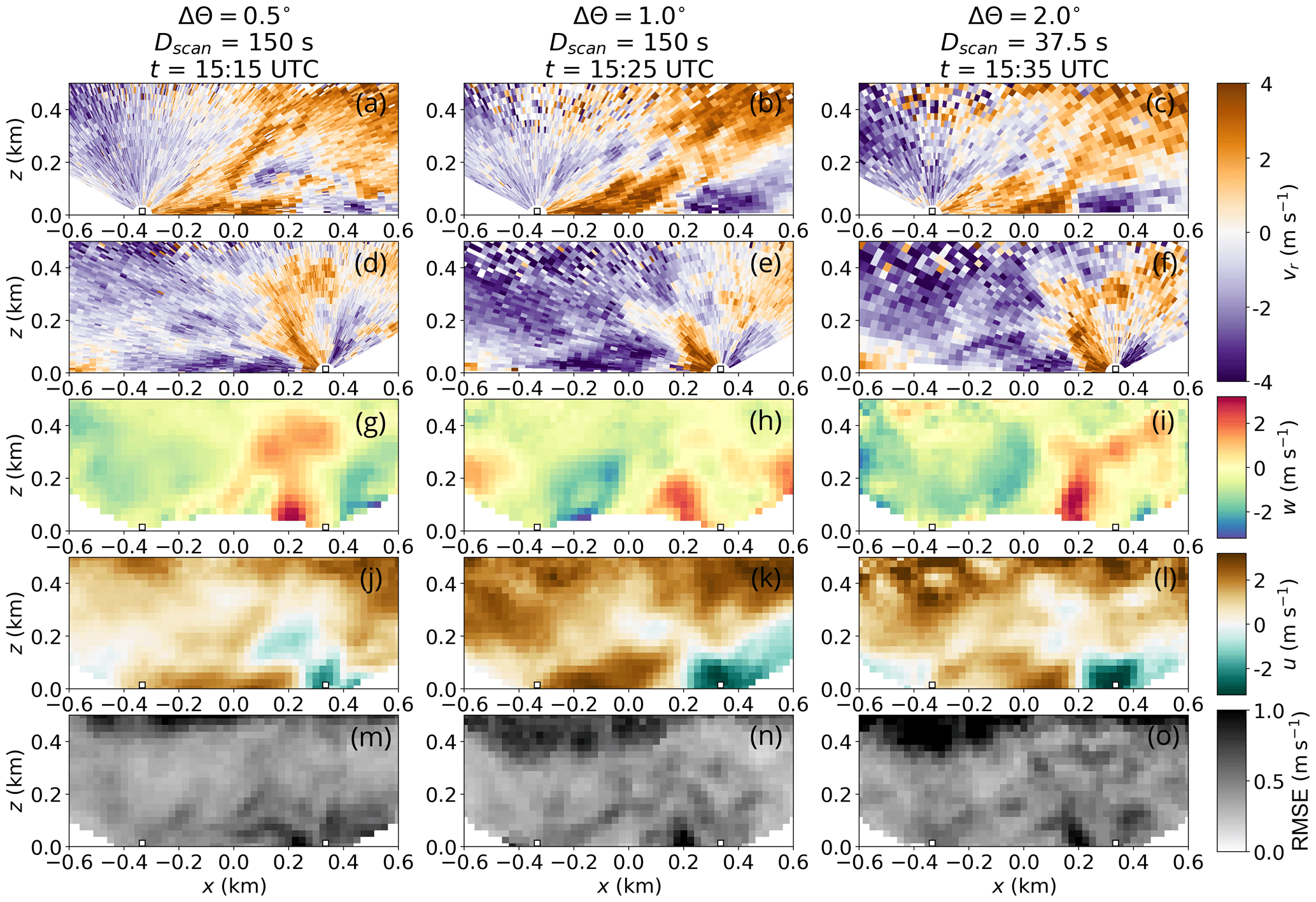
Figure 7 Filtered and temporally interpolated v_r observations, retrieval, and retrieval error obtained for 28 May 2021 between 15:00 and 16:00 UTC at Vaksinen airport. The location of the utilized lidars is indicated by white squares with a black border just above the surface, with lidar₁ in the negative and lidar₂ in the positive x domain in each of the panels. The three columns correspond to the three different scan configurations with configuration-specific Δθ, D_scan, and t (instantaneous cross-section). Each row corresponds to one relevant variable. The first row (a–c) shows processed, instantaneous v_r fields from lidar-37 (here lidar₁). The second row (d–f) shows processed, instantaneous v_r fields from lidar-40 (here lidar₂). The third row (g–i) shows the retrieved w field. The fourth row (j–l) shows the retrieved u field, and the fifth row (m–o) shows the retrieval RMSE field.

Despite a time difference of 10 and 20 min between the different scan configurations, all retrieved fields of u and w indicate the presence of a convective updraft, triggered at around x=200 (Fig. 7g–l). With the retrieved u and w fields and on the basis of the method introduced in Sect. 5.4, we estimated x_up, where the convective updrafts originate at the surface. Figure 8 visualizes the identification process applied to the three retrieved u and v fields which are presented in Fig. 7. Here, the height-averaged w (over the lowest 150 m) reaches a local maximum (w>0.5 m s⁻¹) and u converges (reverses sign from positive to negative with increasing x: $\frac{\mathrm{\Delta }u}{\mathrm{\Delta }x}$) within the grey shaded area for the three tested scan configurations. This area is in fact located around the x=200 mark (Fig. 8d–f).

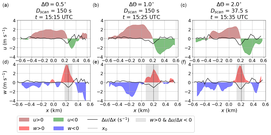
Figure 8 Averaged near-surface (≤150 m) horizontal divergence. The first row (a–c) shows u and the second row (d–f) shows w estimates to visualize the identification process for the near-surface updraft location, x₀. The three columns correspond to the three different scan configurations with configuration-specific Δθ, D_scan, and t (instantaneous cross-section).

For all three scan configurations the maximum w and minimum $\frac{\mathrm{\Delta }u}{\mathrm{\Delta }x}$ fall into almost the same point (x_up) at x=230 m, x=200 m, and x=200 m. Given the meteorological background conditions (see Sect. 6.1 and Fig. 6), buoyancy contributes to the turbulence generation (Ri_f<0) and can be considered the main driver for the observed circulation patterns. Horizontal velocity divergence is expected at the upper edge of the convective updraft to compensate for the upward motion of air. A divergent behavior is, in fact, evident in all three retrieved u fields (Fig. 7j–l) but much weaker than the near-surface convergence. Similar to what was observed by Kunkel et al. (1977), the updraft is attached to the surface and has more of a plume-like character, while at higher altitudes “bubbles” of increased vertical velocities seem to detach.

The near-surface horizontal velocity convergence around x=200 m is already well captured by the v_r fields obtained by lidar-37, which is located at $x=-\mathrm{335}$ m (Fig. 7a–c). The lidars's beam is oriented almost horizontal relative to the near-surface flow field, relevant to the convective updraft and convergence region. Here, angular or spatial resolution does not matter, since even the lowest angular resolution of 2.0^∘ (Fig. 7c) sufficiently captures all relevant features of the horizontal flow. Lidar-40 is located at x=335 m, which is comparably close to the convective updraft region around x=200 m, for all three scan configurations. The region of horizontal velocity convergence, which is not exactly located above lidar-40, is also evident in the horizontally pointing beams (Fig. 7d–f, j–l). Yet here, the updraft strongly contributes to the v_r signal of the vertically or close to vertically pointing beams (Fig. 7d–i).

Within the convectively active region, the RMSE is remarkably similar for all three scan configurations (Fig. 7m–o). It is increased close to the updraft region near the surface (x=200, z<100). The main cause of this increased RMSE is an erroneous estimate of the large w component in the near-surface region. The w contribution to the observed v_r is negligible, since here both lidars observe v_r with predominantly horizontally pointing beams (ill-posed in w). This issue was already addressed by removing any ill-posed w values from the retrieved field (see Sect. 3.2). Above the downdraft region, a larger area of increased RMSE is present for all three scan configurations (upper left corner of the displayed retrieval grid). Here SNR values are decreased (not shown); hence, fewer v_r values are available for the retrieval. The boundary layer depth is horizontally inhomogeneous and particularly increased above the updraft. Hence, the convective updraft directly drives the boundary layer deepening, while the downdraft entrains clear air from the free atmosphere, where uncertainty in the lidar retrieval rapidly increases. Due to its rapid transport of aerosols through the atmosphere, the convective updraft is consequently well suited to be observed with a Doppler lidar.

6.3 Development of a cloud-topped convective structure

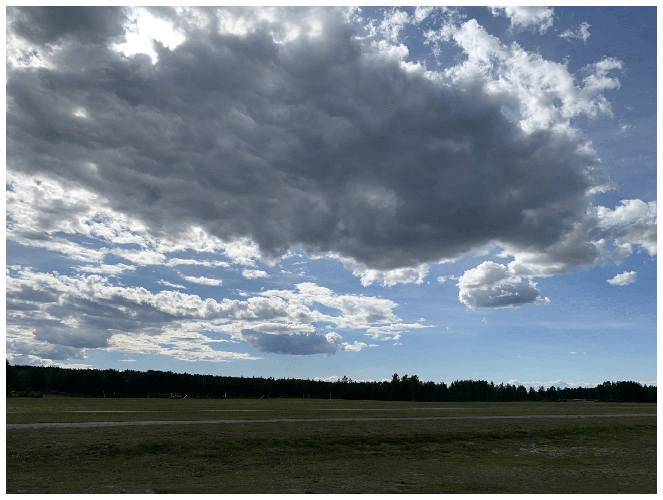
During the Starmoen campaign, we captured a convective day with comparable temperature and humidity development, as well as radiation and turbulent fluxes (Fig. 6). The main differences to the convective day investigated from the Vaksinen campaign are the increased depth of the boundary layer and the formation of convective clouds in the afternoon. The presence of clouds at Starmoen airport on the day of interest is evident from the periods of strongly reduced values of SW_↓ during the afternoon (see Fig. 6). From ca. 13:00 until 14:00 UTC, SW_↓ rapidly fluctuates between diffuse (cloud-shadowed) and nearly clear-sky values, indicating the presence of nonstationary and rather small-scale clouds. From ca. 14:00 to 15:00 UTC, the pyranometer was continuously shadowed by a larger, more stationary cloud (see Fig. 9). At the time the photo in Fig. 9 was taken, the shadow of the cloud covered the entire airfield, though the lidars only capture a finite slice of this cloud within the scanned cross-section as a strong, local increase in SNR at the cloud base.

Figure 9 Cloud observed over Starmoen airport on 29 July 2022 at 14:23 UTC

We estimate the fields of u and w in the vertical cross-section between the lidar on the basis of instantaneous RHI scans (see Sect. 4.2) every 4 min from 14:04 until 14:32 UTC. These fields, as well as the corresponding streamlines and an indication of the cloud base as SNR contours (SNR $>-\mathrm{10}$ dB), are displayed in Fig. 10.

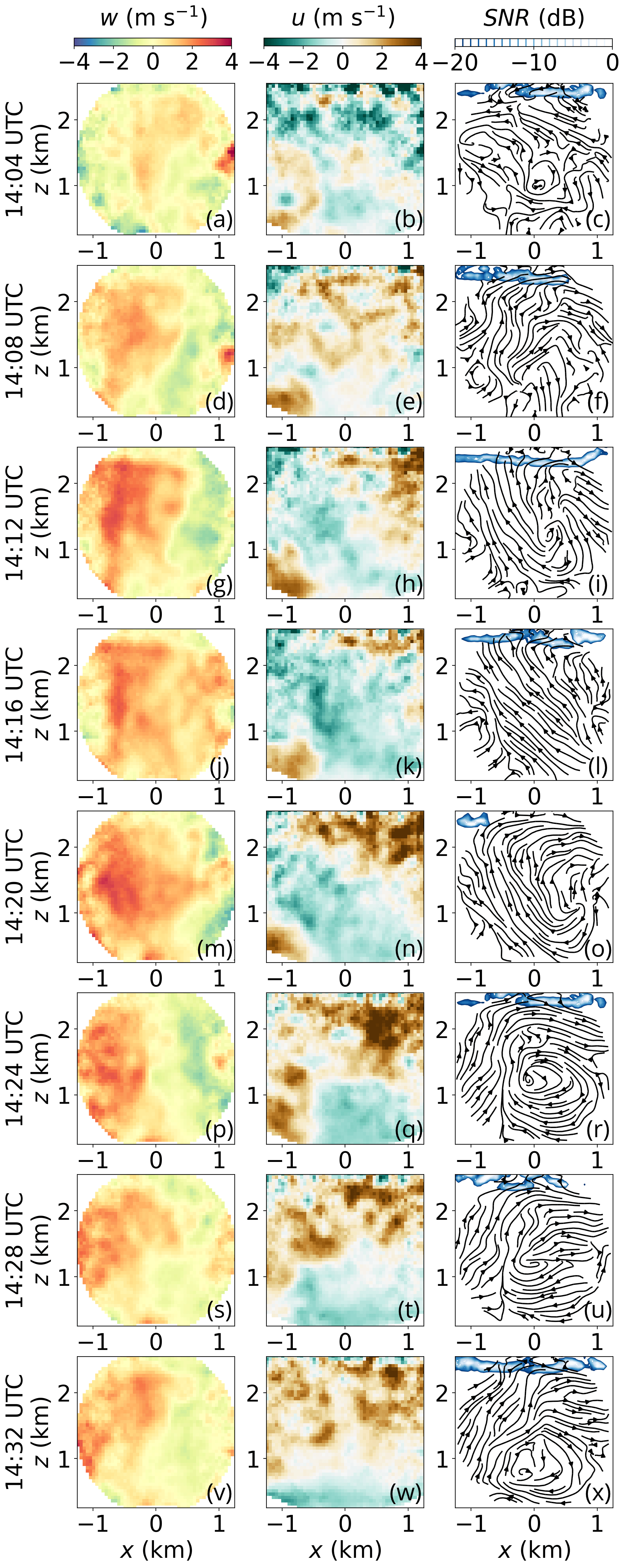
Figure 10 Temporal evolution of convection on 29 July 2022 at Starmoen airport. First column: retrieved w field. Second column: retrieved u field. Third column: streamlines and SNR (cloud backscatter).

The initial velocity fields and streamlines show only weak signs of convection. The velocity patterns indicate predominantly turbulent flow with small-scale fluctuations and no clear convective pattern (Fig. 10a–c). An indication of a cloud is visible above the weak updraft region, which is possibly a remnant of an earlier convective circulation. As time progresses, the velocity clusters intensify, dividing into updraft and downdraft regions (Fig. 10d). Also, the streamlines imply a clearer organization of the flow (Fig. 10f) with less impact of localized and small-scale turbulence indicating the onset of a new, emerging convective circulation. Here, the maximum updraft velocity, $w_{max}^{\uparrow }$, reaches 2.1 m s⁻¹. The updraft terminates just below the cloud base and spans the whole depth of the cloud-topped boundary layer.

The subsequent time steps show further intensification of the updraft and downdraft (Fig. 10g–l), where a converging horizontal velocity pattern in the lower levels focuses into the convective stream into a narrow core of maximum updraft velocity with plume-like characteristics ($x_{\mathrm{up}}=-\mathrm{0.6}$), as also observed by Kunkel et al. (1977). Just below the cloud, a diverging horizontal velocity pattern (Fig. 10h, k) drives the widening of the convective updraft (Fig. 10g, j). Interestingly, the width of the convective stream (Fig. 10i, l) is conserved over the altitude range where horizontal convergence dominates. Here, the streamlines are tilted towards the left-hand side of the cross-section. At 14:12 UTC, $w_{max}^{\uparrow }=\mathrm{2.9}$ m s⁻¹ reaches the maximum value of the displayed series and slightly declines to $w_{max}^{\uparrow }=\mathrm{2.8}$ m s⁻¹ at 14:16 UTC. Here, the updraft cluster (Fig. 10j) is widened substantially in comparison to the preceding time step (Fig. 10g) and spans over nearly the entire width of the cross-section, which is now too narrow and would require Δx (see Table 2) to nearly double to document the complete convective circulation pattern.

The convective circulation further weakens, as entrainment of environmental air and drag forces counteract the effective buoyancy in the following time steps (Fig. 10m–x). The thin core of maximum velocity vanishes and the updraft loses its predominantly plume-like character. Here, the buoyant forcing of the convection begins to break down and only inertia maintains the circulation (see, e.g., Jeevanjee and Romps, 2016). In the last displayed time step (Fig. 10v–x), the cloud is still present, though with no further support from below. The cloud will eventually break down or be advected from the site over time. Here, the streamlines tilt toward the right-hand side of the lidar cross-section with increasing altitude, opposite to the tilt which we observed at the onset of the convective circulation. The boundary layer reached its maximum depth of the day during this hour. Afterwards, radiative forcing, turbulent heat fluxes, and turbulence generation by buoyancy decrease (Fig. 6) and convective activity ceases for that day.

7 Discussion

In the following we discuss the performance of the presented approach and its potential and limitations to sample convection in instantaneous cross-sections of high temporal and spatial resolution. We also discuss and summarize our experiences gained throughout the two presented case studies and interpret the local variability of the convective properties for the two selected sites, as well as the benefit of complementary meteorological observations.

7.1 Lidar setup

We tested the potential of a setup combining two scanning lidars to resolve and characterize atmospheric convection in a vertical plane. The setup will at best be able to retrieve the two-dimensional evolution of the three-dimensional convective flow. Yet, convective circulation is often rather symmetric around its vertical axis (updraft or downdraft) given calm background wind speed conditions (e.g., Emanuel, 1994). In the case of sufficient background wind, the convective structure will be tilted and the cross-section should ideally be oriented parallel to the wind direction to capture the vertical extent of the convective circulation. Furthermore, to interpret the absolute strength and width of the convective updraft or downdraft, the cross-section should pass through the core of the convective structure.

For our setup along the airport runways, we experienced a satisfying hit rate of representative convective circulation patterns during convective conditions indicated by Ri_f even though wind and surface conditions were not necessarily optimal. As the lidars are rather immobile, it is still beneficial to orient the lidars according to the dominant wind direction during convective conditions. To ensure that the setup frequently captures convection, it is also advantageous that the cross-section is placed over surfaces that are likely to trigger the release of thermal updrafts.

Reducing the errors and complications connected to the setup has a substantial impact on the performance of the dual-lidar retrieval. A thorough azimuth calibration of the utilized lidars following the instructions of the lidar manufacturer Leosphere³ prevents unnecessary amplification of out-of-plane v_r errors in the retrieval (see Stawiarski et al., 2013). While synchronization of scan schedules is only of secondary importance (in contrast to Röhner and Träumner, 2013), time synchronization of the lidar-internal clocks is critical. Wrongly matched time stamps are generally hard to identify and correct, yielding amplified errors in v_r retrieval.

7.2 Retrieval and processing

We implement and apply a retrieval algorithm that follows a similar methodology as well-established retrievals for overlapping dual-lidar scans (e.g., Newsom et al., 2008; Cherukuru et al., 2015; Träumner et al., 2015; Haid et al., 2020). We find the best estimate of u and v by solving an over-constrained equation system for each Cartesian point containing several v_r values of both lidars. This reduces the impact of outliers and additionally yields a retrieval error estimate that serves as a measure of confidence for the retrieval in each point.

Generally, the dual-lidar retrieval is quite sensitive to erroneous v_r input, as also discussed by Stawiarski et al. (2013). We found that pre-processing the RHI scans before retrieval has a positive impact on the error reduction and hence on the performance of the dual-lidar approach. The error in v_r connected to noise and erroneous features can be up to an order of magnitude larger than actual values of v_r. As RHI scans are particularly prone to range-folded ambiguities (Bonin and Brewer, 2017), it is crucial to remove these before further processing.

For the lidar observations, the DBSCAN filter (adapted from Alcayaga, 2020) proves to be more effective and accurate than the conventional SNR threshold filter. Applying the DBSCAN filter strongly increases the performance of the dual-lidar retrieval for various conditions. Further processing, in the form of temporal interpolation of the RHI scans, additionally reduces the error compared to using the obtained RHI scans, where θ is dependent on t. From the interpolated scan series, instantaneous scans can be extracted, which reduces the necessity of exact scan schedule synchronization. Also, the interpolation has a larger impact on the temporal error reduction than doubling the temporal resolution of the scans. Since temporal interpolation still has a “blurring” effect on the retrieval, similar to using a temporal radius (see Newsom et al., 2008), it is still beneficial to use a high sampling rate for the scans as the base for the interpolation.

The retrieval based on the processed v_r sections yields a promising representation of the convective circulation for two convective cases. In both cases, convection is well resolved and spans the entire depth of the boundary layer. Consequently, convection contributes substantially to the overturning of heat, moisture, momentum, and aerosols in the convective boundary layer. Convection also contributes to boundary layer deepening or is at least responsible for the maintenance of the boundary layer depth. In particular, the convective updraft and clear evidence of horizontal velocity convergence in the lower part of the convective circulation are captured. This also allows identifying secondary convective parameters, e.g., the origin of the updraft air mass close to the surface, the strength and the size of the updraft, and the horizontal structure of the boundary layer.

7.3 Spatial and temporal resolution

We utilize several scan configurations with various temporal and spatial resolutions. During the first campaign at the Vaksinen site we even tested three different scan configurations. The comparison of the different scanning patterns proved to be challenging, as we cannot be sure whether the differences in observed data are due to changes in the flow conditions or changes in the scan configuration. In particular, the 10 min scanning interval turned out to be too short for the scan configurations with long D_scan (150 s) and did not achieve representative error statistics. To sufficiently compare the scan resolutions, simultaneous observations by an additional lidar would be required. However, we found a solution by artificially decreasing the highest obtained temporal resolution, yielding a representative indication of the impact of the temporal resolution on the error.

It was also not easy to find continuity between the consecutive series of changing scan configurations each 10 min at the Vaksinen site, as the temporal interpolation is only able to produce an entire instantaneous RHI scan after one complete scan. We can only sufficiently resolve the full temporal development of a convective circulation for a continuously sampled series with constant temporal and spatial resolution. As observed for our cloud-topped case, the development of a convective circulation can have a life cycle of the order of several tens of minutes. But there is also an indication for longer-lasting convective patterns for the smaller convective scales obtained at the Vaksinen site.

Still, for the two evaluated cases, all convection relevant scales are well represented, even by the lowest spatial resolution tested within the retrieval grid, which is still in close vicinity of the lidars. It is remarkable that even in the shallow boundary layer case observed at the Vaksinen site, where only smaller-scale convection dominates, the lowest angular resolution is sufficient to resolve the characteristic features of the convective circulation. It is therefore reasonable to use high temporal resolution, even at the cost of spatial resolution or, if the aerosol concentration allows, at the cost of T_scan.

We face a bigger problem to capture the entirety of very large-scale convection that exceeds the boundaries of the retrieval grid in the cloud-topped case. Also, the retrieval becomes less reliable above the cloud base, as the lidar beams can only penetrate a few range gates into the cloud and the data availability drops rapidly. The dual-lidar retrieval is therefore mostly relevant for the dry part of the convective circulation and distance between the lidars should be increased compared to the setup at Starmoen to also capture the largest convective structures.

7.4 Local variability of convective properties

The dual-lidar retrieval complements valuable insights from the surface-based measurements by quantifying the substantial differences in the deepening of the boundary layer by the convective circulation for the case at Vaksinen compared to Starmoen. One potential explanation is the different geographic setting of the locations. The Vaksinen airport is located in a local valley with rather steep topography of approximately 300 m height. This topography potentially enhances the accumulation of cold air in the valley and the development of a nocturnal low-level temperature inversion. In addition, Vaksinen airport is located relatively close to the North Sea, which is a large body of comparably low temperature in May. Cold-air advection from the sea creates an internal boundary layer (Garratt, 1990), which can also contribute to the maintenance of a strong, low-altitude temperature inversion. This inversion is hard to penetrate even for strong updrafts, as observed at the Vaksinen site.

The Starmoen site is much flatter and located far away from any water body of comparable size, and the case features a deeper residual layer from the preceding day. As energy input near the surface and turbulent fluxes increase, convection continuously deepens the boundary layer. The strength of the convective updraft is not stronger compared to the one observed at the Vaksinen site, indicating that there is a weaker inversion. The potential of a deeper boundary layer is indicated, but it is not possible to quantify a weaker inversion without complementary temperature profiles.

7.5 Complementary meteorological observations

With the DBS scan included in the lidar schedules for 10 min each hour, we are able to gain an estimate of the mean profile of the three-dimensional wind. This profile indicates how parallel the flow is towards the evaluated dual-lidar cross-section. Yet, from the dual-lidar retrieval we can clearly observe that the flow during convective conditions is already very complex and nonhomogeneous on small horizontally scales, which is a requirement for an accurate DBS retrieval. As a consequence, the DBS retrieval may not sufficiently capture the profile, in particular with increasing separation of beams with height. Another problem of the DBS scan is that it introduces a discontinuity in the retrieved dual-lidar cross-section time series. In the worst case, the DBS scan is scheduled during a crucial period in the evolution of the convective circulation. As the quality of the DBS retrieval is uncertain, an alternative solution to sample the profile of the three-dimensional wind, which does not interrupt the continuity of the overlapping RHI scans, would be an improvement. A third lidar that scans perpendicular to the dual-lidar setup, creating a “virtual tower” (see Calhoun et al., 2006), could achieve this, for example.

The complementary ground-based measurements, such as those used here, are beneficial to the setup. They can enhance the process of identifying relevant periods for convection and give some indication of the strength and depth of the convection (e.g., Ri_f or a parameter such as the convective velocity scale $w_{*}\sim \stackrel{\mathrm{‾}}{w^{\prime }{\mathit{\theta }}^{\prime }}$ as discussed by Träumner et al., 2011). However, to learn more about the character and physics of the convective boundary layer and evolution of convective circulation (i.e., the impact of drag or moisture on the vertical acceleration), more sophisticated measurements are needed. Background profiles of temperature, humidity, and wind as well as profiles simultaneously measured within the convective updraft to complement the flow field estimates of the dual-lidar approach could significantly improve our understanding of convection, e.g., when evaluated in an empirical model such as introduced by Pálenik et al. (2021). The gLidar project actually aims to achieve such collocated observations.

8 Conclusions and outlook

We presented a dual-lidar setup and retrieval combined with an advanced filtering approach and temporal interpolation to sample and characterize the dynamic properties of atmospheric convection. We demonstrated that our dual-lidar setup and retrieval approach capture the flow field of convective structures projected onto a two-dimensional plane for a clear-sky and a cloud-topped case at two independent sites.

All tested angular resolutions yielded sufficient spatial resolution to resolve the details of the convective circulation, allowing us to prioritize increased temporal resolution. To ensure that the setup captures at least one wavelength of the convective circulation at any point in time, the distance between the two lidars should be increased compared to the presented setups. Utilizing an advanced filter successfully removes erroneous features and noise, yielding spatial continuity in the dual-lidar retrieval. Temporal interpolation further reduces errors that would be amplified in the dual-lidar retrieval and yields an increased temporal resolution. These two processing techniques simultaneously increase data availability while significantly reducing errors compared to conventionally used methods. In particular, these processing techniques enable the estimate of secondary convective parameters, such as the origin, depth, width, and strength of the convective updrafts that contribute to the transport of heat, moisture, momentum, and aerosols, as well as boundary layer deepening or are at least responsible for the maintenance of the boundary layer depth.

Overall, our study presents the potential of a dual-lidar setup as an observational tool to probe the convective flow field. A long-term installation of the setup could provide a sufficient observational basis to validate the representation of convection in LESs, which is used to guide parameterization schemes in weather and climate models. In combination with remote access solutions and processing capabilities, nowcasting of flow conditions, for example for takeoff and landing risk assessments at airports, is feasible. Finally, combining the proposed dual-lidar approach with the observation of additional profiles of temperature and humidity inside and outside the convective updraft offers the potential to gain a deeper understanding of the dynamic processes inherent to convection.