A portable reflected-sunlight spectrometer for CO₂ and CH₄

Mapping the greenhouse gases (GHGs) carbon dioxide (CO₂) and methane (CH₄) above source regions such as urban areas can deliver insights into the distribution and dynamics of local emission patterns. Here, we present the prototype development and an initial performance evaluation of a portable spectrometer that allows for measuring CO₂ and CH₄ concentrations integrated along a long (>10 km) horizontal path component through the atmospheric boundary layer above a target region. To this end, the spectrometer is positioned at an elevated site from which it points downward at reflection targets in the region, collecting the reflected sunlight at shallow viewing angles. The path-integrated CO₂ and CH₄ concentrations are inferred from the absorption fingerprint in the shortwave–infrared (SWIR) spectral range. While mimicking the concept of the stationary California Laboratory for Atmospheric Remote Sensing – Fourier Transform Spectrometer (CLARS-FTS) in Los Angeles, our portable setup requires minimal infrastructure and is straightforward to duplicate and to operate in various locations.

For performance evaluation, we deployed the instrument, termed EM27/SCA, side by side with the CLARS-FTS at the Mt. Wilson Observatory (1670 m a.s.l.) above Los Angeles for a 1-month period in April/May 2022. We determined the relative precision of the retrieved slant column densities (SCDs) for urban reflection targets to be 0.36 %–0.55 % for O₂, CO₂ and CH₄, where O₂ is relevant for light path estimation. For the partial vertical column (VCD) below instrument level, which is the quantity carrying emission information, the propagated precision errors amount to 0.75 %–2 % for the three gases depending on the distance to the reflection target and solar zenith angle. The comparison to simultaneous CLARS-FTS measurements shows good consistency, but the observed diurnal patterns highlight the need to take light scattering into account to enable detection of emission patterns.

1 Introduction

Cities are hotspots for emissions of the greenhouse gases (GHGs) carbon dioxide (CO₂) and methane (CH₄) (e.g., IPCC, 2014; Gurney et al., 2021; Mitchell et al., 2022; de Foy et al., 2023). The major sources are traffic- and heating-related emissions, fossil fuel-based electricity production, natural gas leakages and waste treatment (e.g., Gurney et al., 2019; Sargent et al., 2021; Maasakkers et al., 2022; Huo et al., 2022). At the same time, cities have become a driving force behind climate change mitigation plans and they have committed to ambitious reductions in their greenhouse gas emissions (e.g., Hsu et al., 2019; Wei et al., 2021; Mueller et al., 2021).

To support the evaluation and verification of these emission reduction plans, urban greenhouse gas measurement networks have emerged (e.g., Duren and Miller, 2012; McKain et al., 2015; Turnbull et al., 2019; Turner et al., 2020; Dietrich et al., 2021), measurement campaigns (e.g., Hase et al., 2015; Pitt et al., 2022) have aimed at demonstrating techniques (e.g., Christen, 2014) for emission monitoring and satellite sensors have been shown capable of detecting CO₂ domes (e.g., Reuter et al., 2019; Ye et al., 2020; Kiel et al., 2021) and localized CH₄ leakages (e.g., Maasakkers et al., 2022; de Foy et al., 2023). While the remote sensing tools operated from satellites or ground typically report the column-averaged dry-air mole fractions of CO₂ (XCO₂) and CH₄ (XCH₄), in situ measurements deliver the local concentrations. The former suffer from limited sensitivity to signals confined to the lowermost atmospheric layers and thus require superb precision to detect minute variations. The latter are prone to being affected by local variations, implying limited representativeness on the scale of neighborhoods and city districts. Techniques that average the greenhouse gas concentrations along horizontal paths above cities have been suggested as a tool to bridge the sensitivity gap between in situ and column-averaged data (e.g., Fu et al., 2014; Rieker et al., 2014; Queißer et al., 2016; Griffith et al., 2018). The horizontally integrated concentrations promise better sensitivity to surface emissions than column-averaged data. Simultaneously, they are more representative on kilometer scales than urban in situ data since they average over local emission and turbulence patterns.

The California Laboratory for Atmospheric Remote Sensing – Fourier Transform Spectrometer (CLARS-FTS), stationed on Mt. Wilson in the north of the Los Angeles (LA) Basin at roughly 1700 m elevation, is an observing system that delivers CO₂ and CH₄ concentrations integrated along horizontal path lengths of a few tens of kilometers (Fu et al., 2014). The CLARS-FTS points into the LA Basin, collecting sunlight reflected off the ground from various locations (termed reflected-sun configuration in the following). After reflection, the light propagates at a shallow angle quasi-horizontally through the urban boundary layer towards the observer at Mt. Wilson. From each of the collected absorption spectra, the spectral analysis provides path-integrated CO₂ and CH₄ concentrations. Pointing sequentially at various reflection locations throughout the LA Basin enables horizontal mapping of the urban dome of CO₂ and CH₄ with a resolution on the district scale in a few hours. Since the technique uses sunlight, its operation is limited to daytime and fair weather conditions. The spectral analysis methods need to take into account that there is a quasi-vertical light path component from the sun to the reflection point on the ground in addition to the quasi-horizontal component above the city and that light scattering by particles in the atmosphere complicates radiative transfer considerations (Zhang et al., 2015; Zeng et al., 2017, 2020b). Despite these challenges, the CLARS-FTS has been delivering various insights into the spatiotemporal distribution of CO₂ and CH₄ (and carbon monoxide (CO), nitrous oxide (N₂O) and water vapor isotopologues) above the LA Basin and the related greenhouse gas emission patterns on the ground (Wong et al., 2015, 2016; He et al., 2019; Zeng et al., 2020a, 2021, 2023; Addington et al., 2021).

Here, we present the prototype deployment of a greenhouse gas spectrometer that mimics the observational configuration of the CLARS-FTS but which is portable. Requiring minimal infrastructure, it can be deployed at any location with a vantage point that is elevated above a localized source region and allows for a clear view into the area. The envisaged use-cases are the replication of the CLARS-FTS experiment in places other than LA and the combined deployment of several of these instruments, which would allow for crossed-beam configurations to enhance the horizontal mapping capabilities in a primitive tomographic setup. The instrument, called EM27/SCA, is a derivative of the EM27/SUN FTS, which is in operational use within the Collaborative Carbon Column Observing Network (COCCON) for measuring column-averaged gas concentrations in direct sun configuration (Frey et al., 2019).

Our study is organized as follows. Section 2 outlines the technical developments and calibration procedures required to make the EM27/SCA work in reflected-sun configuration, while Sect. 3 reports on the conditions of co-deployment with the CLARS-FTS in LA. In Sect. 4, we summarize the spectral retrieval of the target gases CO₂, CH₄, CO and, for light path information, O₂ (molecular oxygen). Section 5 discusses the performance of the EM27/SCA and compares it to the simultaneous CLARS-FTS measurements. Section 6 concludes the study with an outlook on future steps.

2 Instrumentation – EM27/SCA

The EM27/SUN FTS (Gisi et al., 2012), commercially available from Bruker Optics, forms the basis of our setup. This compact and portable instrument has been proven to reliably measure XCO₂ and XCH₄ in several field campaigns (e.g., Hase et al., 2015; Butz et al., 2017; Luther et al., 2019, 2022) and is the backbone instrument of the COCCON network (Frey et al., 2019). The FTS has a maximum optical path difference of Δ=1.8 cm, corresponding to a resolution of $\mathrm{1}/\mathrm{\Delta }=\mathrm{0.56}$ cm⁻¹. As the EM27/SUN is designed for direct sunlight observations, we modified several of its components to make it suitable for the fainter radiances expected when measuring sunlight reflected off the ground. Figures 1 and 2, respectively, show a photograph of the instrument during deployment in LA and a schematic of the modified spectrometer. We replaced the standard room-temperature detector module with an extended indium gallium arsenide (InGaAs) detector (Hamamatsu G12183-203K), 2000 times more sensitive and featuring custom-built electronics with a two-stage thermoelectric (TE) cooler set to an operating temperature of −20 ^∘C. The spectral cutoff of the detector and a foil filter mounted in front of it limit the sensitive range to 4000–12 000 cm⁻¹. The 90^∘ off-axis focusing mirror was replaced by one with a 44 mm diameter and an effective focal length of f_eff=33 mm. Given that the diameter of the photosensitive area of the detector diode is 0.3 mm, the full field-of-view (FOV) is 9.1 mrad (0.52^∘). We removed all apertures inside the instrument and mounted an adjustable iris aperture in front of the entrance window. We typically use a beam diameter of 2.6 cm. Together with the fast focusing mirror, this enhances the throughput by a factor of 70. Thus, the more sensitive detector and the increased throughput enhance the sensitivity of the EM27/SCA by a factor ∼10⁵ compared to the standard EM27/SUN.

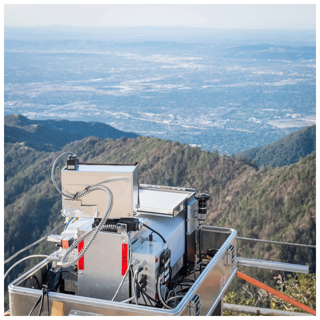
Figure 1 The EM27/SCA instrument on top of Mt. Wilson, overlooking the Los Angeles Basin. The pointing mirrors are located inside the upper metal protective housing, shielding them from direct sunlight. The depicted viewing direction points away from the observer into the basin. The Lambertian reflector plate is mounted on top of the instrument's main body. The context camera is attached on the right.

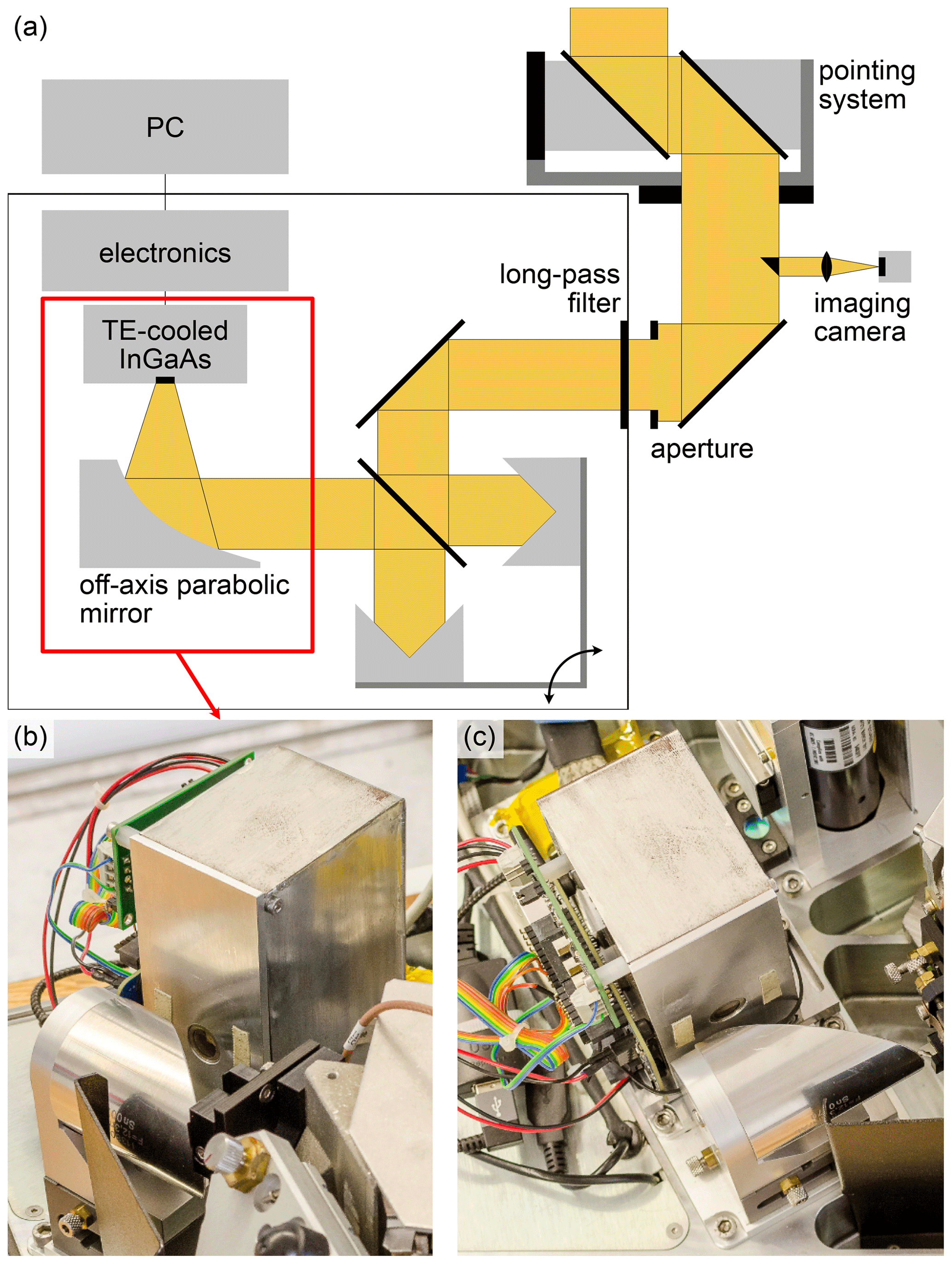
Figure 2 Schematics of the light path through the EM27/SCA (a). Main modifications are the custom detector module (b, c) and the imaging camera recording the FOV. Adapted from Gisi et al. (2012).

In front of the spectrometer, the pointing system (derived from EM27/SUN's “sun-tracker”) collects sunlight reflected from the ground target into the spectrometer. The pointing system is an alt-azimuthal mount consisting of two rotational stages moving two 50 mm elliptic flat mirrors in the azimuthal and zenith directions. Behind the pointing mirrors, a prism couples a small portion of the parallel beam into an imaging camera boresighted with the instrument, allowing for real-time tracking of the instrument's FOV. The FOV camera is a 1/2” CMOS sensor (1280 × 1024 px) with a 900 nm longpass filter and an objective lens with a focal length of f=100 mm, representing the instrument's FOV with a diameter of 181 px. In addition, an identical context camera with a 185^∘ FOV fisheye lens was mounted on the side of the instrument (see Fig. 1), recording the general meteorological conditions and skylight context. Finally, we mounted a horizontally leveled Zenith Lite™ Lambertian reflector plate on top of the EM27/SCA's main body such that reference observations of reflected sunlight without horizontal path component (“short-cut” observations) can be carried out at any time. The diffuse reflectivity of 50 % makes the brightness of the reflector plate comparable to bright ground targets.

2.1 Instrument line shape

We determined the instrument line shape (ILS) of the EM27/SCA from H₂O absorption lines measured in open-path configuration. Following the procedure described in Frey et al. (2015), we averaged 30 min of spectra of a halogen lamp positioned at a distance of 3.2 m while keeping ambient pressure, temperature and humidity conditions constant. From these spectra, we then retrieved the ILS using the LINEFIT software (Hase et al., 1999) with Norton–Beer medium apodization. The FOV of the EM27/SCA is considerably larger than the one of the standard EM27/SUN. However, homogeneous illumination of the FOV is important for an accurate representation of the ILS. We therefore did not point the halogen lamp directly into the instrument but instead observed the homogeneously illuminated reflector plate mounted on top of the instrument (see Fig. 1).

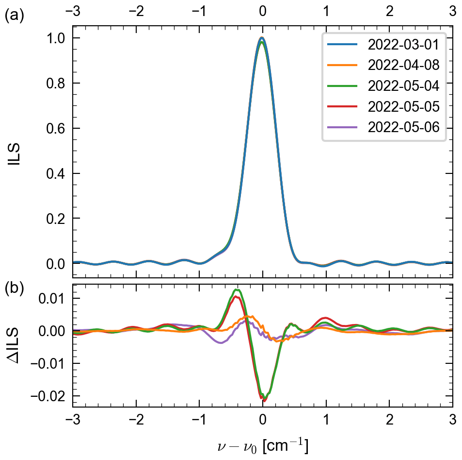
Figure 3 ILS measurements before and during the field campaign at Mt. Wilson. The ILSs (a) are normalized to unity area and subsequently scaled such that the ILS measured on 1 March 2022 has a peak height of 1. Panel (b) shows the differences in the ILS compared to that measured on 1 March 2022. The differences between measurements are within the expected repeatability.

Figure 3 illustrates the ILS and its changes monitored during the course of the measurement campaign in LA reported below. The observed differences are within the expected repeatability of the calibration procedures in the field. The ILS has a full-width-at-half-maximum of 0.54 cm⁻¹ and is slightly asymmetric. Due to the fast optics and larger FOV, the imaging quality of the EM27/SCA is worse and optical alignment is more delicate than for the standard EM27/SUN. Limiting the beam diameter to 2.6 cm as described above clearly improved the width of the ILS and its symmetry.

2.2 Polarization sensitivity

FTS can exhibit sensitivity to the polarization state of the incoming light. This is mainly caused by the beam splitter, as its reflectivity differs for light polarized parallel or orthogonal to the plane of reflection so that the throughput differs for vertically and horizontally polarized light. We characterize the polarization sensitivity of the EM27/SCA by comparing halogen lamp spectra, which are linearly polarized in the vertical or horizontal directions. In the range of 5600–8000 cm⁻¹, the instrument is 8 %–10 % less sensitive to horizontally polarized light than to vertically polarized light. The sensitivity difference increases towards smaller wavenumbers reaching 15 % reduced sensitivity at 4500 cm⁻¹.

2.3 Field of view and scene heterogeneity

In addition to the FOV of 9.1 mrad (0.52^∘) calculated from the optical parameters, we empirically determined (1) the width of the FOV and (2) its position within the image of the FOV camera. To this end, we used a collimated light source with an iris aperture.

To measure the width of the FOV, we scanned the pointing system in steps of 0.1^∘ across the light source positioned at approximately 18 m distance from the spectrometer. Figure 4 shows the intensity mapping with the nominal FOV overlaid. The width of the measured FOV is in good agreement with the nominal FOV of 0.52^∘ and only slightly elongated along the zenith direction. Note that the FOV rotates with changes in azimuth viewing direction. To determine the FOV position within the FOV camera image, we positioned the light source approximately 33 m away from the instrument. We determined the pointing direction corresponding to the maximum signal. We then scanned in the azimuth and zenith directions until the signal dropped by one-half. From this, we determined the center position of the light source in the camera image as the average position of all half-maximum positions and recorded an image pointing there. We determined the center pixel of the instrument FOV inside this image from fitting an ellipse to the saturated pixels. The off-center position of the camera in the beam together with the finite distance of the light source leads to a parallax error. The camera is placed 2.5 cm from the beam axis. From this we estimated the error to be 10 % of the full FOV (0.05^∘). Additionally, we observed that the FOV drifts over the course of 1 day. The drift is limited to below 0.1^∘ and is most likely caused by thermal expansion of the pointing system.

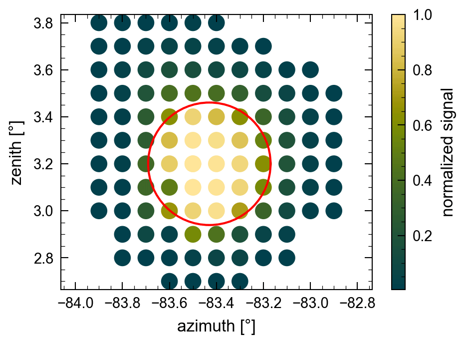
Figure 4 Mapping of the FOV of the EM27/SCA by scanning over a point source. The nominal FOV is marked with a red circle around the estimated center.

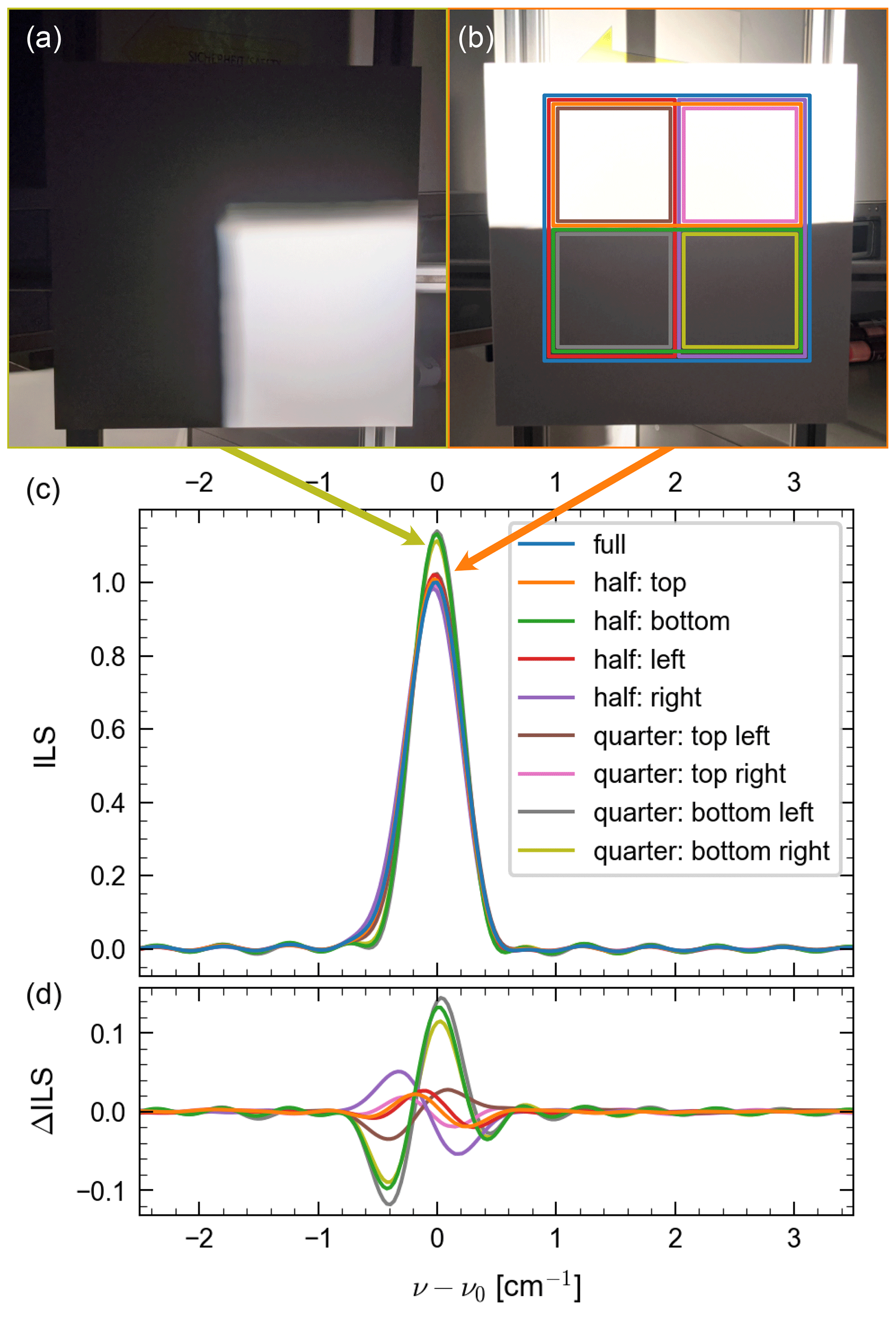
Figure 5 Test configuration (a, b) and ILS measurements (c) for an inhomogeneous illumination of the reflector plate. The variations in the ILS under different illumination patterns show that the instrument is influenced by scene inhomogeneity in extreme cases.

Real-world scattering targets are only approximately homogeneous. To determine the influence of scene heterogeneity on the ILS, we set up a laboratory experiment using a 50 × 50 cm Lambertian reflector plate located at a distance of 7 m from the EM27/SCA. A halogen lamp illuminated the reflector plate homogeneously. We conducted various experiments by shading parts of the reflector plate such that only one-half or one-quarter of the area was illuminated (Fig. 5a, b). For each configuration, we recorded the ILS according to the procedure outlined in Sect. 2.1. Figure 5c and d show the distortions of the ILS caused by inhomogeneous illumination. Clearly, we observe changes in the width and the peakedness of the ILS, with narrower and more-peaked ILS occurring when the lower part of the reflector plate was illuminated. Note that the orientation of the image depends on viewing direction, since the image rotates with azimuth viewing direction.

We conclude that the ILS of the EM27/SCA is sensitive to scene heterogeneity. However, the checkerboard pattern used for laboratory testing is certainly an extreme configuration. Thus, we expect the effect to be smaller for typical targets in the field. Nevertheless, we took care of selecting homogeneous targets for our field deployment in LA.

3 Field deployment in Los Angeles

To evaluate the performance of the EM27/SCA, we deployed it side by side with the CLARS-FTS during a period of roughly 1 month. We positioned the EM27/SCA adjacent to the CLARS-FTS on a small viewing terrace at the Mt. Wilson Observatory at 1670 m a.s.l. overlooking the Los Angeles Basin (Fig. 1). We took measurements over 26 d in the period from 7 April to 5 May 2022, pointing at up to nine targets in the northern LA Basin with slant distances of up to 25 km (see map in Fig. 6).

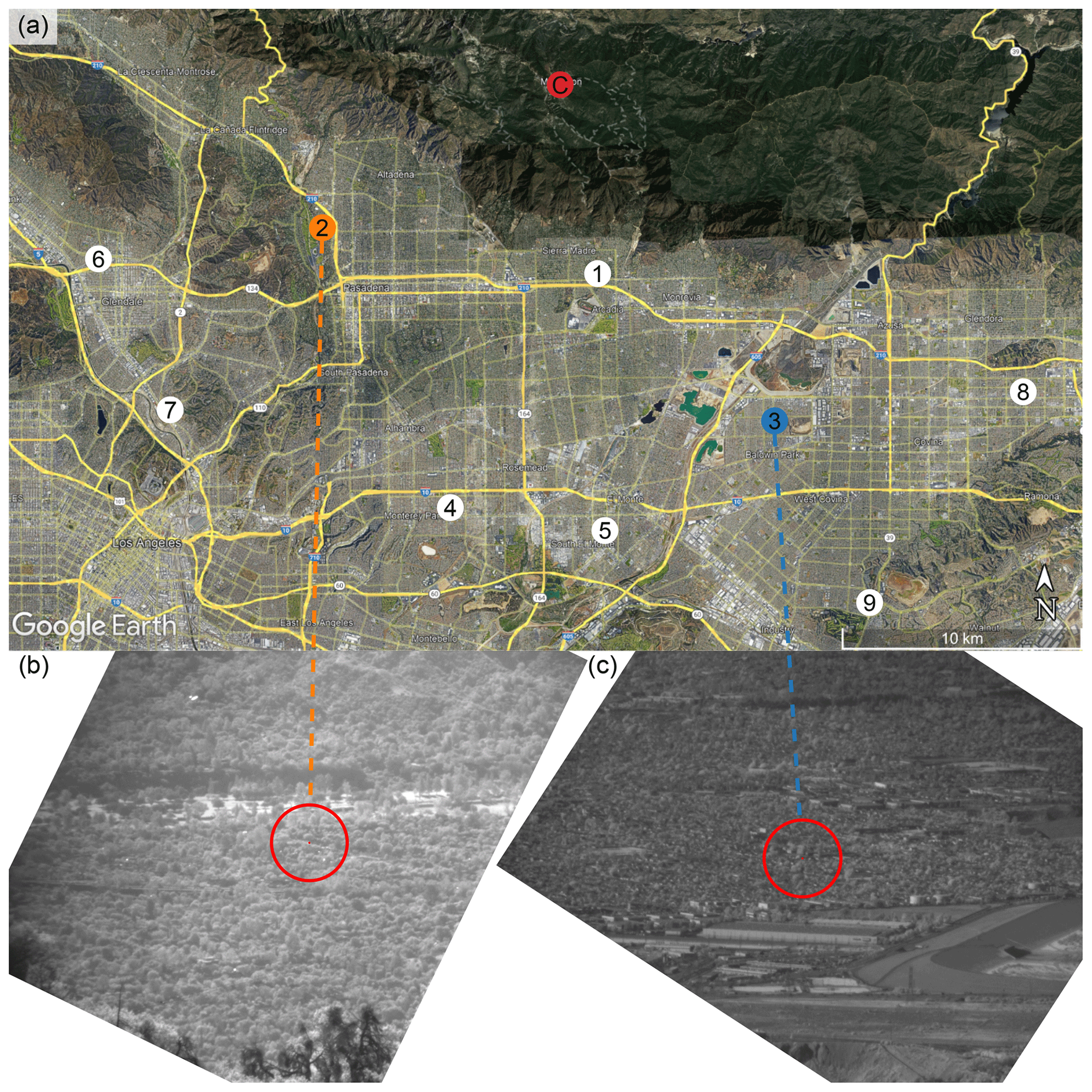
Figure 6 Location of the CLARS-FTS on Mt. Wilson (C) and ground scattering targets (numbers) in the LA Basin. The lower panels show FOV camera images of the West Pasadena (WP) (2, b) and Baldwin Park (BP) (3, c) targets. The instrument FOV is marked with a red circle.

A typical measurement cycle started with a short-cut measurement of the reflector plate and then, cycled through the ground targets in the basin, including one additional short-cut measurement. We co-added 10 interferograms (at an interferogram sampling frequency of 10 kHz) per target resulting in roughly a 12 min duration for a full cycle of nine ground targets plus two reflector measurements. In the later part of the campaign, we recorded three spectra per target, with 10 interferograms each, increasing the duration of a full cycle to 36 min. The early phase of the campaign was dedicated to testing the setup and finding the best measurement configurations and therefore, over a few days, a cycle covered only a single or a few ground targets (instead of the total of nine) and one reflector measurement. On three days, we only conducted reflector measurements since a marine cloud layer covered the basin. Simultaneously with the spectrometer recording interferograms, the FOV camera captured an image of each target scene in each cycle and the context camera recorded an image of the overhead sky.

The pointing directions for each target were determined at the start of the campaign via the FOV camera of the CLARS-FTS. As discussed in Sect. 2.3, special care was taken that the target scenes were homogeneous, i.e., not exhibiting strongly contrasted features across the FOV. However, in an urban setting, perfectly homogeneous targets are not available. GPS coordinates of the targets are available through the pointing calibration of the CLARS-FTS (Fu et al., 2014). After target selection, the EM27/SCA was pointed to the same targets as CLARS-FTS via direct comparison of the FOV images.

For our initial demonstrator assessment in Sect. 5, we focus on the two targets West Pasadena (WP) and Baldwin Park (BP), which have the most revisits. These targets represent urban ground with houses, as visible in Fig. 6. The targets have a slant distance of 11.5 (WP) and 16.4 km (BP).

4 Spectral retrieval

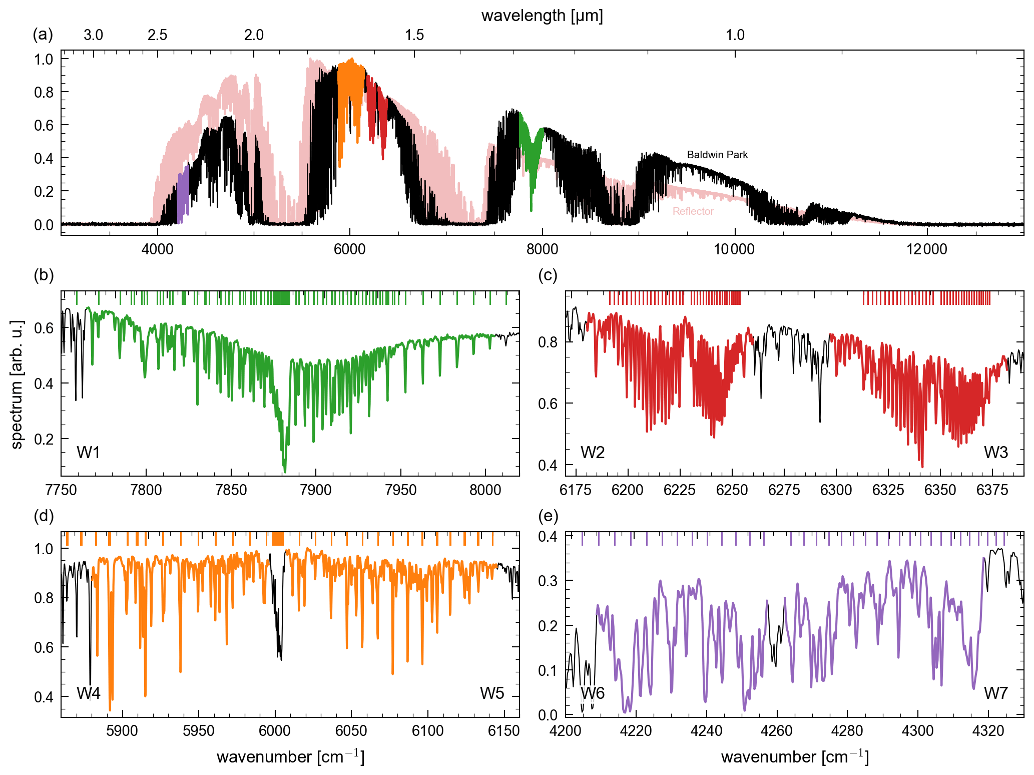
Figure 7 Typical reflected-sun spectrum of the BP target around 15:50 LT (at SZA 46.6^∘). (a) shows the full spectrum with the retrieval windows highlighted in color. A reflector spectrum from roughly the same time is plotted in the background. The other panels show the retrieval windows for CO₂ (red, c), CH₄ (orange, d), CO (purple, e) and O₂ (green, b). Note that CO is a weak absorber and that W6 and W7 are dominated by CH₄ and H₂O absorption lines.

The EM27/SCA recorded DC-coupled interferograms, which we converted to absorption spectra via a Fourier transform using the preprocessor of the PROFFIT retrieval software routinely employed for EM27/SUN processing within the COCCON network (Frey et al., 2019). Throughout this study, we used the Norton–Beer medium apodization. The processing included a DC correction that corrected the interferograms for mild brightness fluctuations during recording. Together with the spectra, we stored the height of the center burst of the interferograms as well as a measure for DC fluctuations. Later, we used this data to identify spectra suffering from cloud contamination and oversaturation.

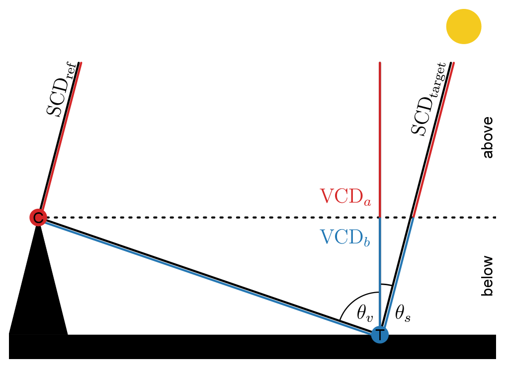
Figure 8 Representation of the viewing geometry as implemented in the retrieval. We separate the model atmosphere at instrument level, scaling the VCDs above instrument level in reflector and below instrument level in target retrievals. From the resulting VCDs we derive the total SCDs for reflector (SCD_ref) and target (SCD_target) measurement. Finally, we calculate VCD_a from SCD_ref and VCD_b from the difference between SCD_ref and SCD_target (see Eq. 3).

Figure 7 shows a typical absorption spectrum measured with the EM27/SCA and highlights the absorption bands used for the retrievals of CO₂, CH₄, CO and O₂. We submit the absorption spectra to a variant of the RemoTeC radiative transfer and retrieval algorithm to infer the gas abundances. RemoTeC has been designed for satellite measurements of XCO₂, XCH₄ and XCO in the SWIR spectral range (Butz et al., 2011). The variant we employed here has been modified to accommodate the particular observation geometry (see Fig. 8) by dividing the layered, horizontally homogeneous model atmosphere into an overhead part, i.e., the part of the atmosphere above the instrument stationed at Mt. Wilson, and a boundary layer part, i.e., the part of the atmosphere below the instrument where the targets in the LA Basin are located. For the overhead part, the forward model calculates the one-way downward slant transmittance of sunlight at instrument level. For the boundary layer part, the forward model corresponds to the two-way transmittance between instrument level and the level of ground reflection taking into account the solar zenith angle (SZA, θ_s) and the viewing zenith angle (VZA, θ_v). Combining the overhead and boundary layer transmittances yields the forward model simulating the expected measurements for the LA Basin targets. For short-cut measurements of the reflector plate, only the overhead part is relevant.

We set up the retrieval such that a least-squares estimator delivered vertical column densities (VCDs) of the target absorbers. We regularized our retrieval such that each absorber had one degree of freedom in the vertical. For reflector measurements, we scaled the overhead VCDs. For target measurements, we varied the partial VCDs in the boundary layer part, while the overhead part was imposed by the a priori. The following performance analysis makes further use of slant column densities (SCDs) defined as

$$\begin{array}{}\text{(1)}& \mathrm{SCD}=\mathrm{VCD}\times \mathrm{AMF},\end{array}$$

where AMF is the air mass factor: the ratio of the slant path through a layer to the vertical depth of the layer. As such, the AMF is different for the parts above (AMF_a) and below (AMF_b) instrument level. They are defined via

$$\begin{array}{}\text{(2)}& {\mathrm{AMF}}_{\mathrm{a}}={\displaystyle \frac{\mathrm{1}}{\cos \left({\mathit{\theta }}_{\mathrm{s}}\right)}},{\mathrm{AMF}}_{\mathrm{b}}={\displaystyle \frac{\mathrm{1}}{\cos \left({\mathit{\theta }}_{\mathrm{s}}\right)}}+{\displaystyle \frac{\mathrm{1}}{\cos \left({\mathit{\theta }}_{\mathrm{v}}\right)}}\end{array}$$

under our geometric assumptions (cf. Fig. 8). Analyzing the SCDs is useful because they are directly related to optical thickness, and with it to the spectra, making them a good quantity for the performance evaluation of the EM27/SCA.

VCDs offer the advantage that geophysical variation is deconvolved from changes in the geometric light path. However, they incorporate geometric assumptions, which in our case differ above and below instrument level (cf. Eq. 2). This non-uniformity throughout the model atmosphere makes total VCDs difficult to interpret, because an increase in the SCD below instrument level has a much smaller effect on the VCD than the same increase in the SCD above instrument level. To circumvent this problem, we evaluated the partial VCDs above (VCD_a) and below (VCD_b) the instrument separately. VCD_a are directly calculated from the reflector measurements. VCD_b are derived from the differences between the SCDs from the target (SCD_target) and the reflector (SCD_ref), taking into account AMF_b.

$$\begin{array}{}\text{(3)}& {\mathrm{VCD}}_{\mathrm{a}}={\displaystyle \frac{{\mathrm{SCD}}_{\mathrm{ref}}}{{\mathrm{AMF}}_{\mathrm{a}}}},{\mathrm{VCD}}_{\mathrm{b}}={\displaystyle \frac{{\mathrm{SCD}}_{\mathrm{target}}-{\mathrm{SCD}}_{\mathrm{ref}}}{{\mathrm{AMF}}_{\mathrm{b}}}}\end{array}$$

To calculate VCD_b, we interpolated SCD_ref between reflector measurements bracketing the time of the target measurement. VCD_b is the quantity ultimately of interest and also the quantity our target measurements are most sensitive to.

Table 1 Overview of retrieved and assumed parameters; detailed description in the main text.

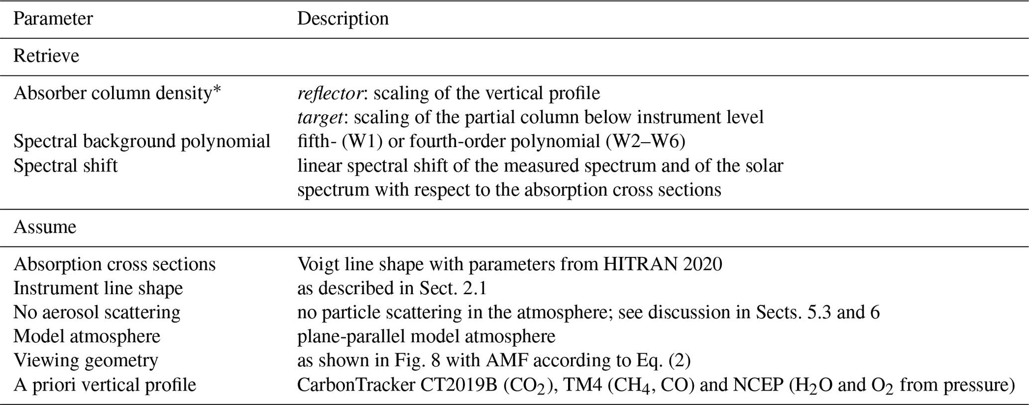
^∗ Absorbers are listed in Table 2.

Note that, for the initial assessment of the instrument performance, we did not consider scattering by particles in the forward model, as also previously assumed by Fu et al. (2014). This is also the basis for our choice of regularization described above. While we scale the vertical absorber profile for reflector measurements, for target measurements we expect the largest variability below instrument level. For one, this layer contains a large portion of the light path and the emission signal we aim at. Secondly, variability due to unaccounted aerosol scattering originates there (cf. Fig. 14 and the discussion in Sects. 5.3 and 6). Thus, it is reasonable to attribute all variability to the lowest layer rather than scale the total column. In particular, since we only use total SCDs in the further analysis (cf. Eq. 3), errors in the a priori profile above instrument level are compensated for in the lowest layer. The remaining error is caused by attributing the molecules in the total column to regions with different pressure and temperature. We summarize the retrieved parameters and assumptions in Table 1.

Table 2 Retrieval windows.

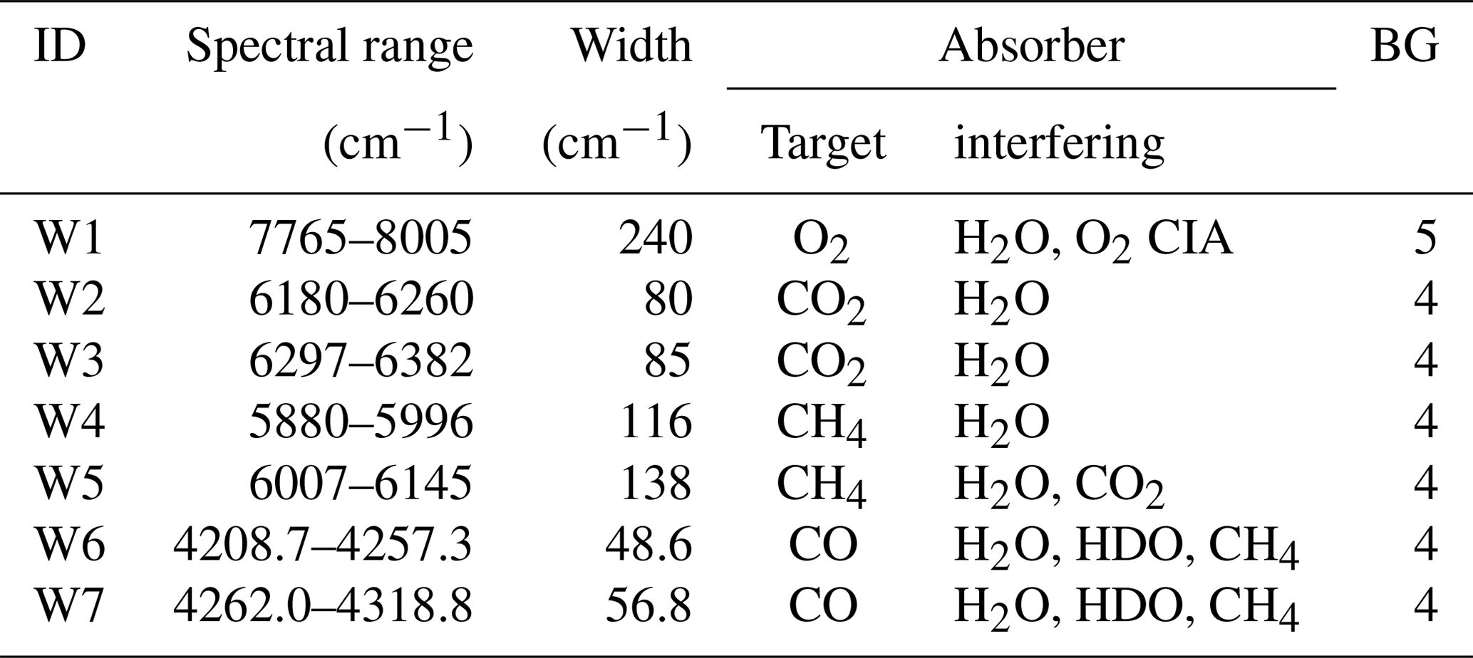
BG: spectral background polynomial order. CIA: collision-induced absorption.

Table 2 lists the spectral windows (see also Fig. 7) from which we retrieved the O₂, CO₂, CH₄ and CO VCDs. Absorption cross sections for all species were calculated from spectroscopic parameters using a Voigt line shape and the HITRAN 2020 database (Gordon et al., 2022). In W1, we include a pseudo-absorber accounting for the O₂ collision-induced absorption (CIA). All absorbers were retrieved independently for each window. Note that windows W4 and W5 excluded the CH₄ Q-branch, as we found systematic errors in retrievals including it. For windows W6 and W7, we found that retrieving the main H₂O isotopologue and HDO independently reduced fitting residuals. In all other windows the H₂O cross sections included lines of all isotopologues scaled with their standard abundance. Broadband variation in the spectrum baseline was accounted for through fitting a spectral background polynomial together with the gas VCDs. Since we neglect aerosol scattering, the polynomial represents the scene brightness but is not strictly the surface albedo. The polynomial is of the fourth order in W2 to W7 and the fifth order in the largest window W1. We computed the solar spectrum from the empirical line list by Toon (2015), which was also used by Coddington et al. (2021) for the computation of the TSIS-1 HSRS.

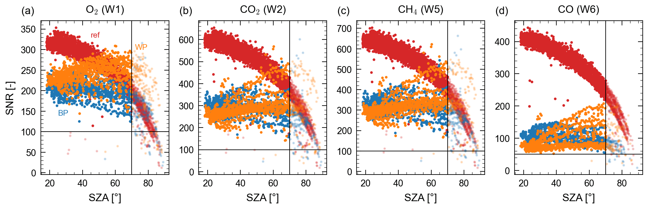
Figure 9 SNRs for spectra measured between 7 April and 5 May 2022 plotted against SZA for the reflector (red) and the targets BP (blue) and WP (orange).

RemoTeC used a priori profiles from CarbonTracker CT2019B (Jacobson et al., 2020) for CO₂ and TM4 (Meirink et al., 2006) for CH₄ and CO. Water vapor (H₂O) and oxygen (O₂) a priori profiles were calculated from NCEP meteorological data (NCEP, 2000), which also provided the vertical pressure and temperature profiles. The pressure at instrument level was taken from the CLARS weather station (Fu et al., 2014) and was used as the lowest pressure level for the reflector measurements as well as for dividing the atmosphere in the overhead and boundary layer part in the case of the target measurements.

To exclude unreliable measurements, we applied a series of filters to all measurements. We did not analyze spectra recorded at SZA greater than 70^∘ and filtered measurements with a signal-to-noise ratio (SNR, defined in Sect. 5) of less than 100 in W1–W5 and less than 50 in the CO retrieval windows. Only few measurements were removed due to low SNR in W1–W5 (0.2 %), while 4 % of the measurements were excluded from CO retrievals in W6 and W7. Additionally, the CO retrieval did not fully converge for 18 % of the measurements. These measurements were still used for retrievals of species from the other windows. We further filtered for cloud contamination by utilizing the DC component of the interferogram, as proposed by Klappenbach et al. (2015). Since the DC component changes with temporal variations in sunlight intensity, its variability increases when the sun is partially obstructed. We calculated the variability DC_var as the fraction of the maximum value (DC_max) to the minimum value (DC_min) of the baseline and subtracted one so that no variability corresponds to a value of zero.

$$\begin{array}{}\text{(4)}& {\mathrm{DC}}_{\mathrm{var}}={\displaystyle \frac{{\mathrm{DC}}_{\max }}{{\mathrm{DC}}_{\min }}}-\mathrm{1}\end{array}$$

The cutoff value of this filter was empirically determined to be 0.03 from cloud-free measurements, identified with the help of the context camera. This filter removed 7 % of the measurements.

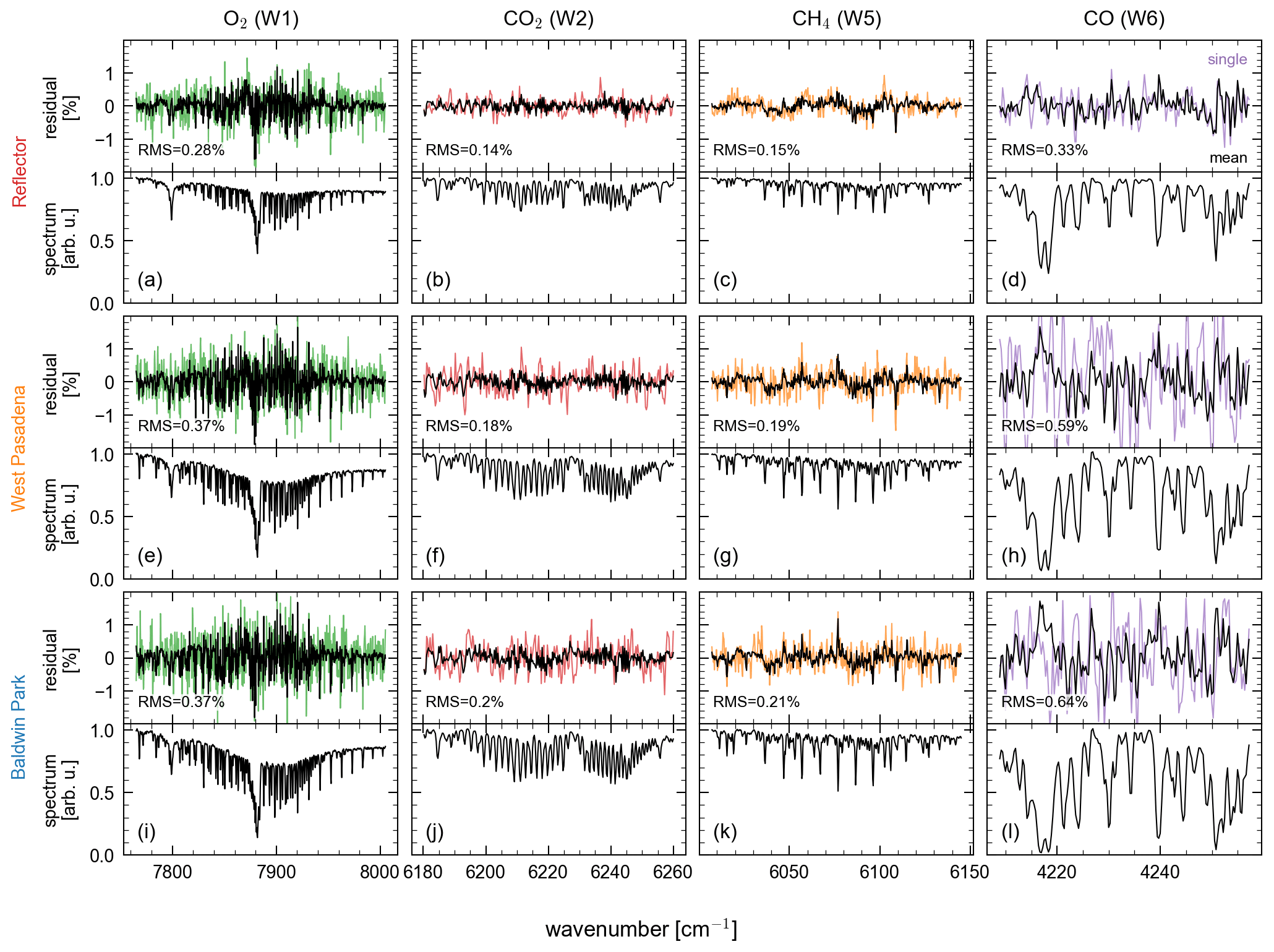
Figure 10 Spectra and spectral residuals for the reflector (a–d), target WP (e–h) and target BP (i–l) for the W1 (O₂, green, a, e, i), W2 (CO₂, red, b, f, j), W5 (CH₄, orange, c, g, k) and W6 (CO, purple, d, h, l) windows. The lower subplots in each panel show a single spectrum; the upper subplots show a residual from the single spectrum (colored) and a full-day average (black) of 124 (reflector), 124 (WP) and 122 (BP) normalized residuals (119, 112 and 112 for CO).

5 Performance

5.1 Signal-to-noise ratio and spectral residuals

To evaluate the performance of the EM27/SCA, we start with calculating the spectral SNR for the retrieval windows defined in Table 2 and illustrated in Fig. 7. The SNR is the ratio of the maximum transmittance in the respective window to the out-of-band noise. The latter was calculated as the standard deviation in the spectral range 2500–3056 cm⁻¹, where there is zero throughput of the spectrometer system. Generally, the SNR depends on multiple factors including the spectrally variable optical throughput, sensitivity of the detector, reflectivity of the target, spectral solar irradiance, position of the sun in the sky and atmospheric conditions. Figure 9 shows the SNR in dependence of SZA for spectra of the reflector and the two targets BP and WP.

Typical SNRs range from 200–400 for target measurements and 400–600 for reflector measurements. The SNR for the reflector measurements is most compact and follows a clear dependence on SZA since these measurements, being conducted at high elevation and having zero horizontal path, approximate direct sun conditions. The SNR of the target measurements shows more scatter and no compact SZA dependency, which points at the strong influence of atmospheric conditions, atmospheric scattering effects and the geometry of surface structures. For the O₂ window (W1), the generally greater surface reflectivity compensates for the reduced detector sensitivity compared to the CO₂ (W2, W3) and CH₄ windows (W4, W5) of the targets. The CO retrieval windows (W6, W7) exhibit lower SNR, on the order of 50–150, as the windows are located towards the longwave cutoff of the InGaAs detector. Note that the SNR in the CO retrieval windows is generally lower for WP than for BP. We attribute the upward SNR trends with increasing SZA for WP to atmospheric scattering towards the evening.

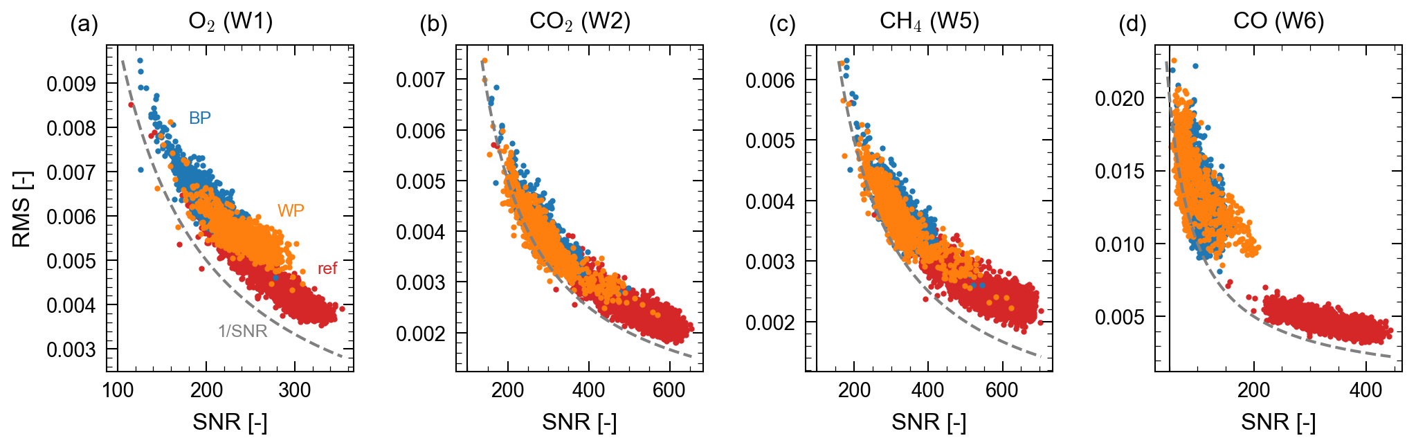
Figure 11 RMS of the spectral residuals for measurements between 7 April and 5 May 2022 plotted against SNR for the reflector (red) and the BP (blue) and WP (orange) targets.

Processing the acquired spectra with RemoTeC (see Sect. 4) yields best-fit simulated spectra. They allow for inspecting the spectral fitting residuals, defined as the differences between the measured spectra and the best-fit simulations. Figure 10 shows the spectral residuals for one window of each species, averaged over a whole day of observations. For averaging, each residual was normalized by the maximum measurement signal in the respective window. Due to the averaging, noise is negligible and the spectral residuals reveal systematic errors due to deficiencies in the retrieval simulations, such as forward model approximations and parameter errors. The residuals and their root-mean-square (RMS) for the reflector measurements are generally smaller than for the targets in the LA Basin. This points at contributions from the neglect of atmospheric scattering, which is a better approximation for the reflector than for the target measurements. Further, spectroscopic uncertainties, such as line shape errors, typically grow with the length of the light path, as absorption lines become more opaque and thus target spectra might be more affected than the reflector measurements. Individual spectral structures correlate with the positions of H₂O lines (e.g., at 5892, 5940, 6020, 6226, 6242, 6305, 6325, 6334 and 6363 cm⁻¹), suggesting spectroscopic errors. The fitting residuals in the O₂ window (W1) are larger and more systematic than for CO₂ (W2, W3) and CH₄ (W4, W5). Despite revisiting our calibration procedures, taking into account spectral variation in the ILS and performing various sensitivity runs, we were not able to identify the cause for this.

Figure 11 evaluates the RMS of the spectral residuals against SNR. Generally, the RMS follows the 1 / SNR pattern expected from a noise-dominated measurement for both reflector and target spectra. However, there is an offset that comes from the systematic residual structures, which are particularly pronounced in the O₂ band.

Overall, the spectral performance of the EM27/SCA is promising in terms of retrieving precise CO₂, CH₄ and O₂ columns. For CO, the spectral cutoff of the detector and the low surface reflectivity around 4250 cm⁻¹ imply a small SNR. A next-generation instrument might consider detectors and optics with better performance at the longwave end of the SWIR spectrum.

5.2 Precision

To estimate the measurement precision we empirically evaluate the precision of the retrieved SCDs for each gas (as explained in Sect. 4). We evaluated measurements from a 4 d period of the early campaign, where the sampling of the evaluation targets was densest. We calculated the precision error as the standard deviation σ of the ratio between each measurement and a rolling average,

$$\begin{array}{}\text{(5)}& \mathrm{\Delta }\mathrm{SCD}=\mathit{\sigma }\left({\displaystyle \frac{{\mathrm{SCD}}_i}{\langle \mathrm{SCD}{\rangle }_t}}\right),\end{array}$$

where ΔSCD is the estimated relative precision error of the SCDs, SCD_i is the slant column density of measurement i and 〈SCD〉_t is the rolling average SCD. We chose an averaging interval of t=30 min, corresponding to seven measurement cycles, as a trade-off between convolving actual geophysical variability into our precision estimates and considering a sufficient number of samples for calculating the average SCDs. Figure 12 shows the ratio of the SCDs to their rolling average against SZA, as well as the histograms. Table 3 lists the resulting relative precision errors for the various absorbers. For CO₂, CH₄ and O₂ SCDs we find a relative precision of 0.36 %–0.55 % without a distinct dependency on SZA. The precision for CO SCDs is considerably worse, as expected from the low SNR in windows W6 and W7 and the weakness of the CO absorption signal. To test the robustness of these estimates, we repeated the analysis with rolling averages over 20 min (five cycles) and 40 min (nine cycles), which resulted in only small changes (Table 3).

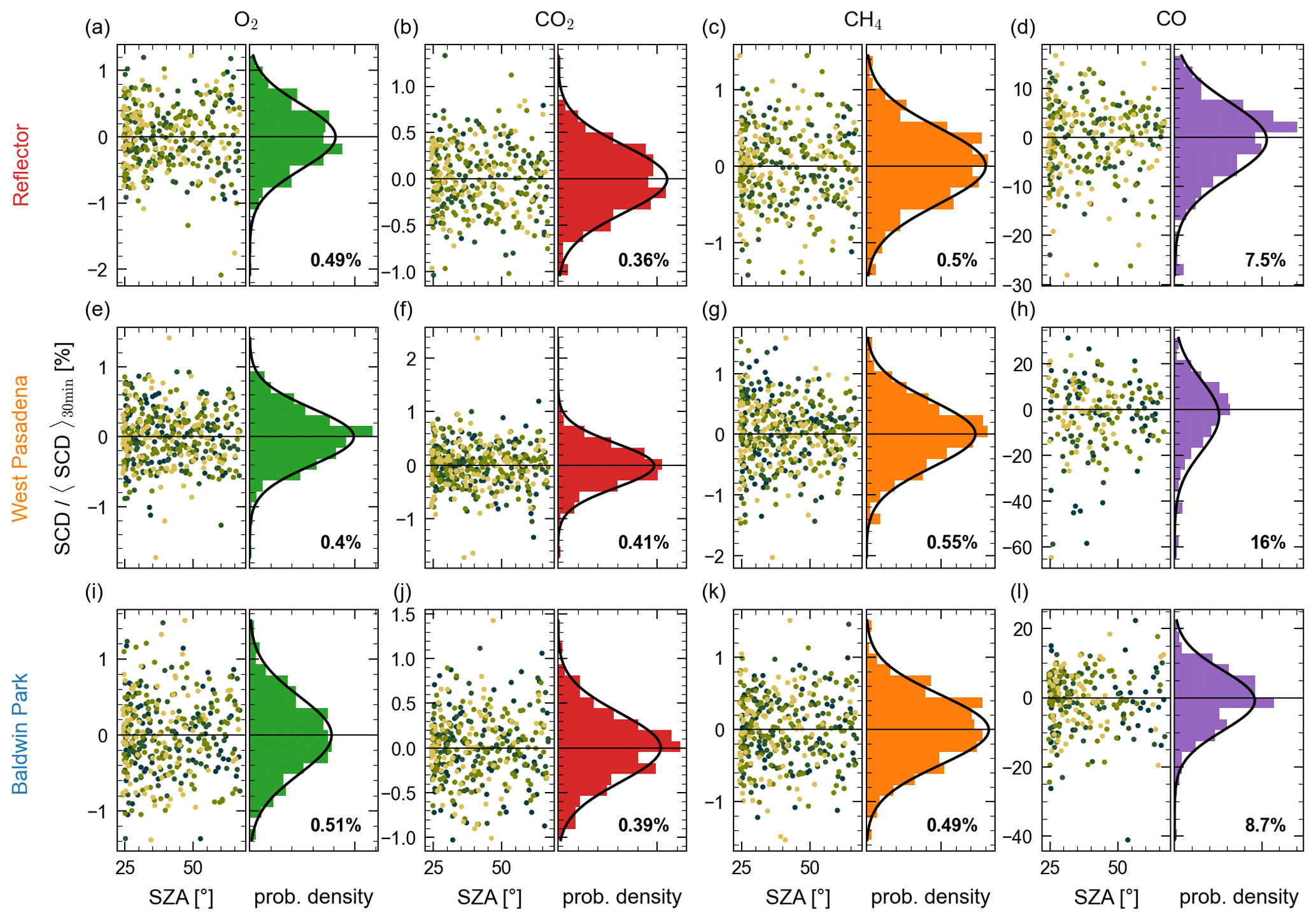
Figure 12 Departures of O₂ (a, e, i), CO₂ (b, f, j), CH₄ (c, g, k) and CO (d, h, l) SCDs from their 30 min rolling average, plotted against SZA (left subpanels) and as histograms (right subpanels), including a normal distribution with the corresponding mean and standard deviation for the reflector and the WP and BP targets. The scatterplots are color coded by day.

Table 3 Relative precision error of the absorber SCDs estimated from the departures of individual measurements from a 30 min rolling average. Numbers in parentheses show the last digit changes when repeating the analysis with 20 and 40 min rolling averages.

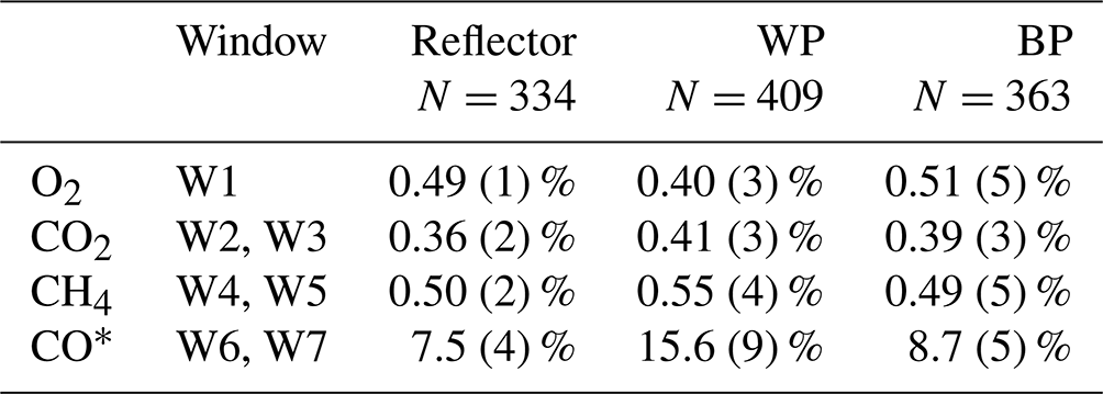
^∗ N is lower for CO retrievals: 261 (reflector), 177 (WP), 232 (BP).

5.3 Comparison to CLARS-FTS

To assess the consistency of the EM27/SCA measurements compared to those of CLARS-FTS, we submitted the CLARS-FTS spectra of the same targets, WP and BP, and the CLARS-FTS reflector to the RemoTeC retrieval with analog settings as for the EM27/SCA spectra. We interpolated the higher-precision CLARS-FTS partial VCDs in time to EM27/SCA measurement instances and subsequently calculated the CLARS-FTS SCDs. Evaluating all the reflector measurements in the campaign period, we found that CLARS-FTS SCDs differ from EM27/SCA SCDs on average by a factor 1.046 for O₂, 1.0068 for CO₂, 1.014 for CH₄ and 0.997 for CO. Such scaling factors might originate from the different spectral resolutions of the EM27/SCA (0.56 cm⁻¹) and the CLARS-FTS (0.2 cm⁻¹) as Gisi et al. (2012) found in comparisons between the Total Carbon Column Observing Network (TCCON) and EM27/SUN. For all the following analyses, we scaled the EM27/SCA retrievals by these factors.

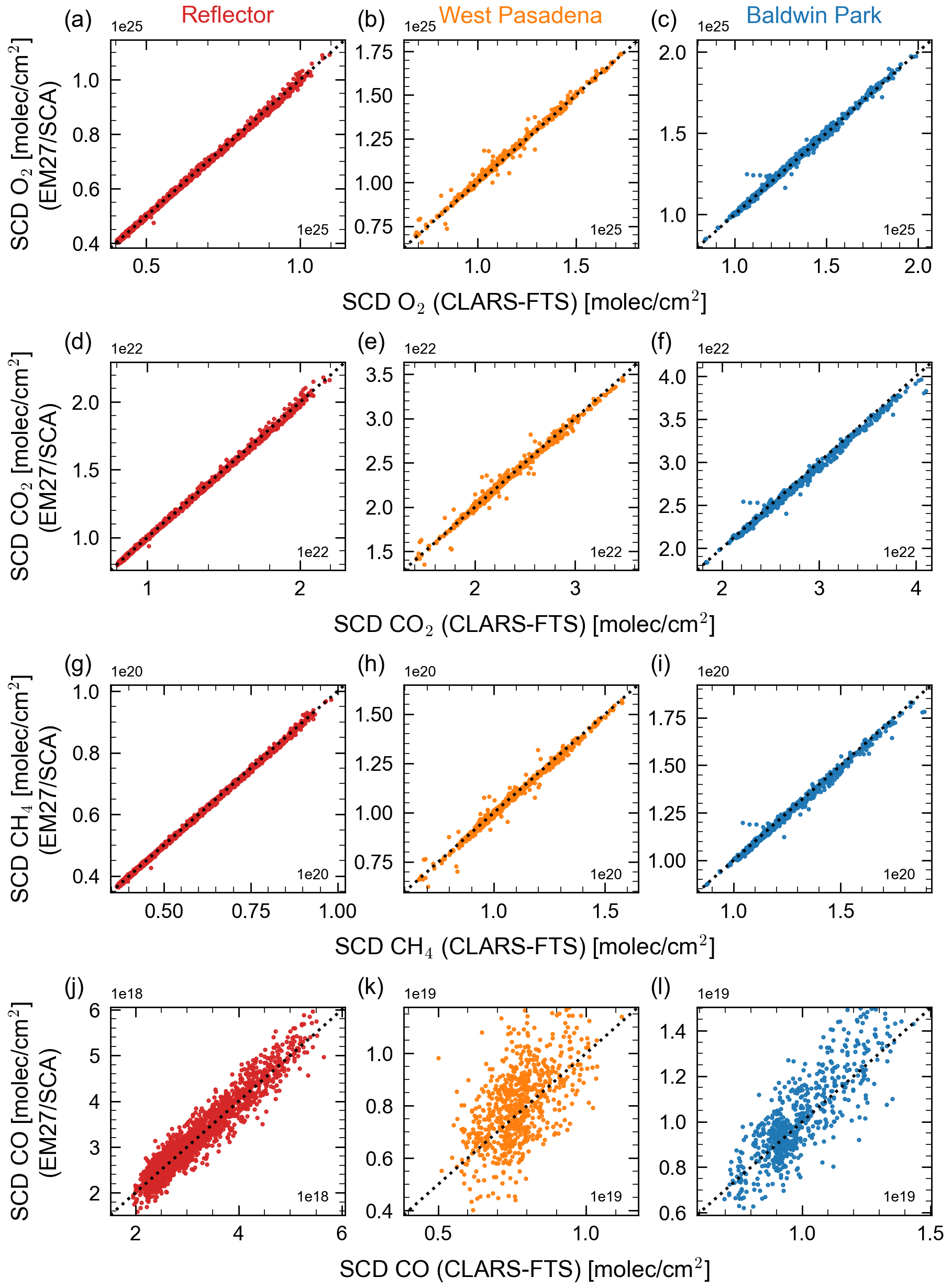
Figure 13 Correlation of O₂, CO₂, CH₄ and CO SCDs (top row to bottom row) between EM27/SCA and CLARS-FTS for reflector (red, a, d, g, j), WP (orange, b, e, h, k) and BP (blue, c, f, i, l) measurements. The dotted lines show the 1:1 relationship.

Figure 13 shows the correlation between the EM27/SCA and CLARS-FTS retrievals. Measurements of the reflector and both targets show a good correlation in O₂, CO₂ and CH₄ with correlation coefficients near 1. CO shows a decent correlation for reflector measurements. For target CO measurements, low precision dominates.

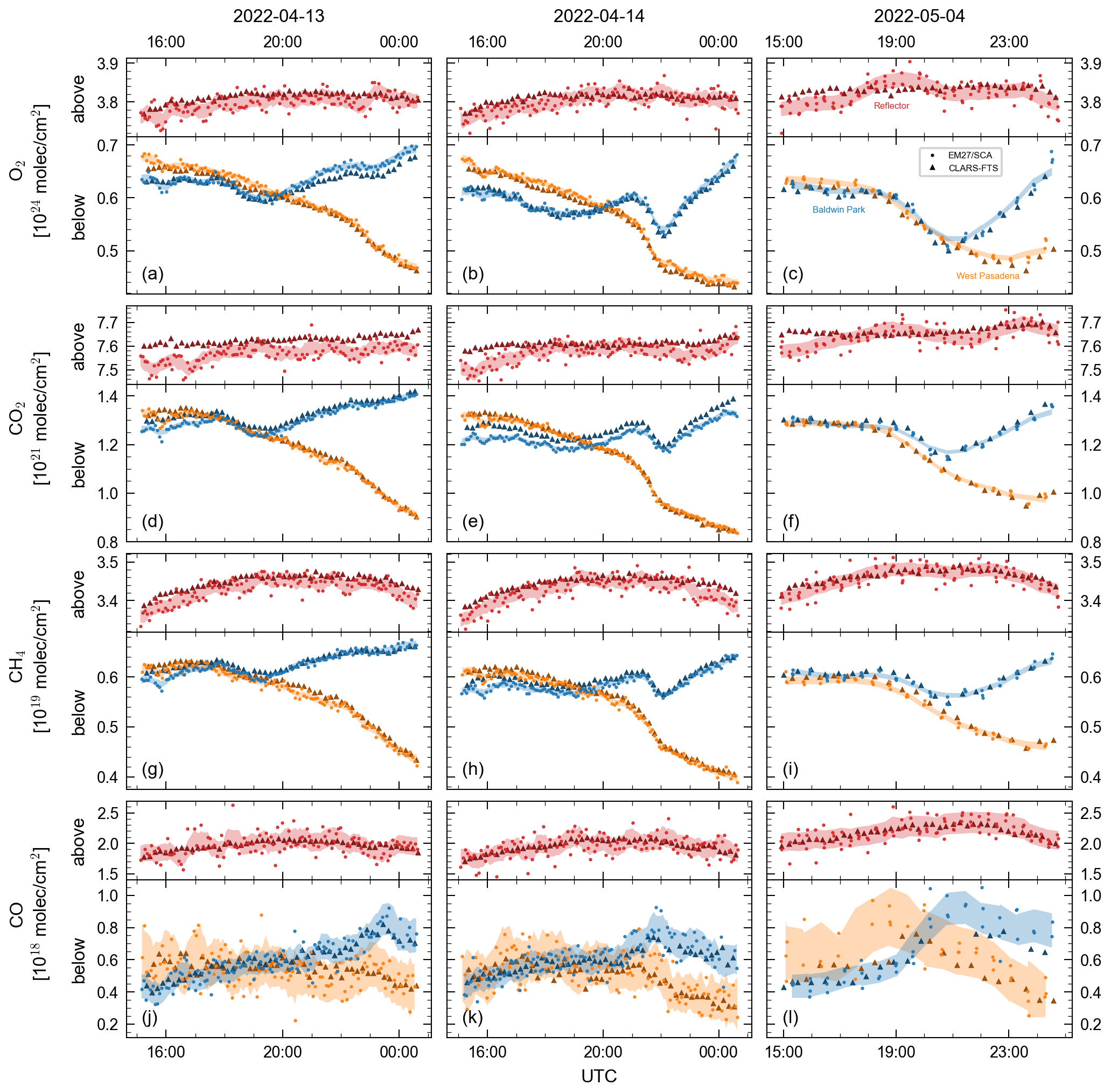
Figure 14 Time series of the VCD_a (above instrument level) and VCD_b (below instrument level) of O₂, CO₂, CH₄ and CO (top tow to bottom row) measured by the EM27/SCA (dots) and the CLARS-FTS (triangles). Three illustrative days are shown: 13 April 2022 (a, d, g, j), 14 April 2022 (b, e, h, k) and 4 May 2022 (c, f, i, l). The partial VCD_a is retrieved from reflector measurements (red). The VCD_b below instrument level is derived from the difference of WP (orange) and BP (blue) from the reflector measurement. The EM27/SCA precision error is displayed as shading around the rolling average. The first two days belong to the period where we cycled through three targets only, and therefore, these days show a higher sampling rate.

Figure 14 shows the observed diurnal variations in the O₂, CO₂, CH₄ and CO partial VCDs above (VCD_a) and below (VCD_b) instrument level for the EM27/SCA and CLARS-FTS for three illustrative days. We calculate the precision error of the partial VCDs via Gaussian error propagation from the relative precision of target and reflector SCDs (Table 4). Since the fraction of the light path below instrument level depends on target distance and SZA, the precision error for target measurements increases for closer targets and higher SZAs.

Focusing on the overhead reflector measurements first (red symbols in Fig. 14), we find that the two instruments generally agree well for all four absorbers and that the VCD_a are not very variable during the day and from day to day, as expected for the quasi-direct sun geometry. Generally, the CLARS-FTS has substantially better precision than the EM27/SCA as expected from the CLARS-FTS evaluation by Fu et al. (2014). The standard deviations of the differences between EM27/SCA and CLARS-FTS VCD_a amount to 1 % for O₂, CO₂ and CH₄ and to 7 % for CO. There are some systematic deviations, especially in the early morning hours, for CO₂ and, although weaker, also for O₂ and CH₄. For these species, the EM27/SCA records show a low bias on 13 April, and on 5 May there is a diurnal variation on the order of the precision error, which is not present in the CLARS-FTS data. For CO, the large scatter masks possible systematic differences.

Turning the focus to the VCD_b in the boundary layer below instrument level (orange and blue symbols in Fig. 14), we generally find that O₂, CO₂ and CH₄ show strong diurnal variations with amplitudes exceeding 10 % of the VCD_b. These variations are present in O₂ and strongly correlated between species, thus pointing to the influence of light scattering by aerosols. Since aerosol scattering effects are unaccounted for in our retrieval, the presence of aerosols implies a forward model error that shows up as VCD underestimation if scattering induces light path shortening and vice versa for light path enhancement compared to our geometric light path assumption. While these atmospheric scattering effects have large implications for how to interpret the data (Zhang et al., 2015), the VCD_b from EM27/SCA and the CLARS-FTS are largely consistent. For the BP target (blue symbols in Fig. 14), there are systematic deviations of the EM27/SCA records from the CLARS-FTS data, e.g., for O₂ in the evening and for CO₂ in the morning of 13 April and for CO₂ throughout the day of 14 April. These systematic deviations are less pronounced for the WP target. After extensive sensitivity studies, we speculate that scene heterogeneity for the BP target may contribute to these deviations. Scene heterogeneity can be variable during the day due to the changing illumination conditions of the ground scene. As explained in Sect. 2.1, heterogeneous illumination of the target affects the ILS of the EM27/SCA, which in turn induces errors in the gas retrievals if the ILS distortion is not accounted for. Due to the lower spectral resolution of the EM27/SCA, the effect on the retrievals is larger than for the CLARS-FTS since the overall impact of the ILS is larger for low resolution than for high resolution.

Table 4 Relative precision error range for VCD_a and VCD_b on 13 April.

6 Discussion and conclusion

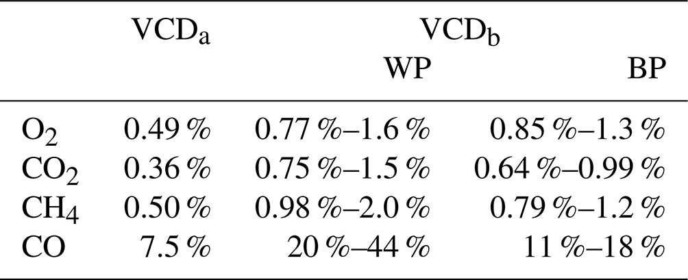
Our study discusses the prototype design and performance of the EM27/SCA FTS. The instrument concept is based on the direct sun EM27/SUN FTS, but it achieves manifold higher sensitivity, making it suitable for measurement of sunlight reflected by ground targets of opportunity. While being portable, the instrument mimics the observation concept of the CLARS-FTS stationed at Mt. Wilson looking downward into the LA Basin. Our performance evaluation during a 1-month side-by-side deployment with the CLARS-FTS shows that the precision errors for the SCDs of CO₂, CH₄ and O₂ retrieved from EM27/SCA measurements are on the order of 0.5 %, which translates into errors of 0.7 to 2 % for the partial VCDs in the layer below instrument level (VCD_b) in the LA Basin, somewhat depending on the ground reflection target. For CO, precision errors for the SCDs are in the range from 7 to 16 %, translating into errors of several tens of percent for the VCD_b of the targets in the LA Basin. Thus, while performance is promising for detecting urban enhancements of CO₂ and CH₄, the EM27/SCA requires reduction in the noise level in the CO channel (around 2.350 nm).

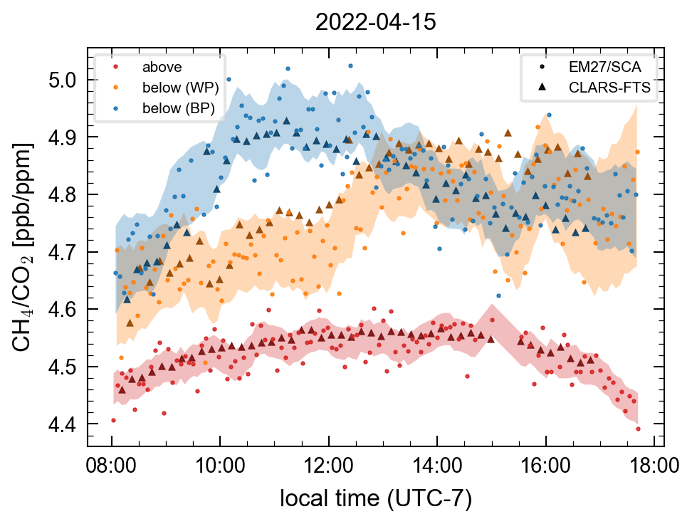
Figure 15 Single day of ${\mathrm{CH}}_{\mathrm{4}}/{\mathrm{CO}}_{\mathrm{2}}$ ratio measurements show a CH₄ enhancement in the Los Angeles Basin assuming a constant CO₂ background (Wong et al., 2015).

As previous studies for CLARS-FTS (Zhang et al., 2015; Zeng et al., 2017) and our Fig. 14 show, the particular viewing geometry, with a long horizontal light path component exceeding 10 km through the urban boundary layer of LA, causes light scattering by aerosols to be the dominant source of variation in the retrieved VCD_b if aerosol effects are neglected in the gas retrievals. To correct to the first order for these scattering effects, the column-averaged dry-air mole fractions X_i of gas i can be calculated via

$$\begin{array}{}\text{(6)}& {\mathrm{X}}_i={\displaystyle \frac{{\mathrm{SCD}}_i}{{\mathrm{SCD}}_{\mathrm{REF}}}}\times {\mathrm{X}}_{\mathrm{REF}},\end{array}$$

where REF denotes a reference gas whose dry-air mole fraction X_REF is known a priori. The idea is that aerosol scattering effects induce the same relative errors in the spectral retrievals of species i and REF, and thus the effects cancel in Eq. (6). Using O₂ as a reference gas is appealing since its dry-air mole fraction is well known and constant for all relevant purposes here. However, Zhang et al. (2015) show that using O₂ as reference gas results in erroneous corrections since the O₂Δ band is spectrally distant from the retrieval windows of the target gases CO₂, CH₄ and CO. Thus, spectral variation in the aerosol and ground scattering properties make the radiative transfer in the O₂ windows different from the other windows. In contrast, ratioing CH₄ with CO₂ from the neighboring spectral windows better compensates for the radiative transfer effects. Figure 15 illustrates a case where the ${\mathrm{CH}}_{\mathrm{4}}/{\mathrm{CO}}_{\mathrm{2}}$ ratio for BP in the morning has a substantial enhancement compared to the data for WP and the reflector. The NOAA High-Resolution Rapid Refresh dataset (Dowell et al., 2022) indicates southwest-to-west wind conditions at wind speeds increasing from 1 to 5 m s⁻¹ over the course of the day. Following studies of CLARS-FTS (Wong et al., 2015, 2016), we argue that this is a geophysical signal related to emission and transport patterns in the LA Basin. Major CH₄ point sources are located southwest of the BP target (see Fig. A1). However, in order to relate the ${\mathrm{CH}}_{\mathrm{4}}/{\mathrm{CO}}_{\mathrm{2}}$ patterns to CH₄ emissions and their transport, according to Eq. (6), we would require assumptions on the reference XCO₂. Additionally, source attribution would require atmospheric transport modeling. We also tentatively identify the increase in the ${\mathrm{CH}}_{\mathrm{4}}/{\mathrm{CO}}_{\mathrm{2}}$ ratio around 12:00 to 13:00 local time for the West Pasadena target in TCCON measurements at the California Institute of Technology (CalTech) (Wunch et al., 2011; Wennberg et al., 2022) (see Fig. A2), located 5 km south of the WP target. The magnitude of the ${\mathrm{CH}}_{\mathrm{4}}/{\mathrm{CO}}_{\mathrm{2}}$ signal differs substantially so that despite the high precision of the TCCON measurements, the signal is on the same order as the scatter. While the scatter in the EM27/SCA data is significantly larger, the signal is clearly observable. This illustrates the value of the reflected-sunlight measurement geometry.

The use of the ${\mathrm{CH}}_{\mathrm{4}}/{\mathrm{CO}}_{\mathrm{2}}$ ratio has been discussed in depth for the CLARS-FTS measurements (Wong et al., 2015, 2016; He et al., 2019; Zeng et al., 2023), and we will follow up on such cases in future studies. Furthermore, we plan to develop a simultaneous retrieval of GHGs, aerosol properties and surface albedo. For this, we will need (1) an absolute calibration of the spectra and (2) adjustments to our radiative transfer model. Despite RemoTeC being able to retrieve aerosol properties in the satellite viewing geometry with the observer on top of the atmosphere, the radiative transfer model is not flexible enough to achieve this for an observer inside the atmosphere. Overcoming this limitation is in principle possible but would be a major effort and is beyond the scope of this instrument performance evaluation. Additionally, polarization effects could become important. If they have a significant impact on our retrieval, we need to account for the EM27/SCA polarization sensitivity and make an assumption on the polarizing properties of the surface. We will follow up on this in future studies.

Assuming that atmospheric scattering effects can be reliably corrected, the VCD_b errors listed in Table 4 and shown in Fig. 14 directly yield a limit for detectable enhancements of the respective gas abundances in the LA Basin. Verhulst et al. (2017) found typical local enhancements in the LA boundary layer in the range of 17–31 ppm CO₂ and 140–220 ppb CH₄. Zhang et al. (2015) estimated 10–20 ppm XCO₂ enhancements for CLARS-FTS measurements of the WP target by calculating the differences between CLARS-FTS Spectralon and LA TCCON measurements. Zeng et al. (2021) showed typical enhancements of 20 ppm in XCO₂ and 150 ppb in XCH₄ retrieved from CLARS-FTS measurements with the GFIT3 full physics algorithm. Assuming background mole fractions of 420 ppm for CO₂ and 1900 ppb for CH₄, these typical enhancements amount to relative variations of 5 % (CO₂) and 8 % (CH₄), and thus they are greater than our VCD_b errors. When they occur in a correlated pattern, e.g., due to transport effects such as shown in Fig. 15, the EM27/SCA is able to reliably measure them.

Our analysis suggests further instrument refinements. Enhancing the signal-to-noise ratio would be required for useful CO measurements, and it would be generally beneficial for more reliable measurements and lower detection limits for all the gases. Section 2.1 highlights that the alignment of the detector optics is cumbersome and that the ILS is somewhat asymmetric, which we mainly relate to the detector optics being optimized for throughput, accepting inferior focusing quality as trade-off. Further, we find that the ILS of the EM27/SCA is sensitive to inhomogeneous illumination of the FOV (Sect. 2.1), and in Sect. 5, we speculate that residual systematic differences between the EM27/SCA and CLARS-FTS might be related to scene inhomogeneity. Thus, a next-generation instrument should consider improved detector optics and homogenizing the FOV.

The largest potential for improvement lies in the explicit integration of aerosol scattering in the retrieval algorithm, as shown by Zeng et al. (2021). This would most likely improve fit quality, reduce uncertainty and pave the way for reliable measurement of near-ground CO₂ and CH₄ concentrations.

Appendix A

Figure A1 CH₄ point sources as registered in the California Air Resources Board inventory (CARB, 2023). Point size signals CH₄ emission strength, color corresponds to the ${\mathrm{CH}}_{\mathrm{4}}/{\mathrm{CO}}_{\mathrm{2}}$ emission ratio for the respective CH₄ source.

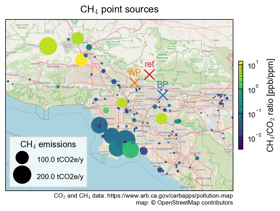
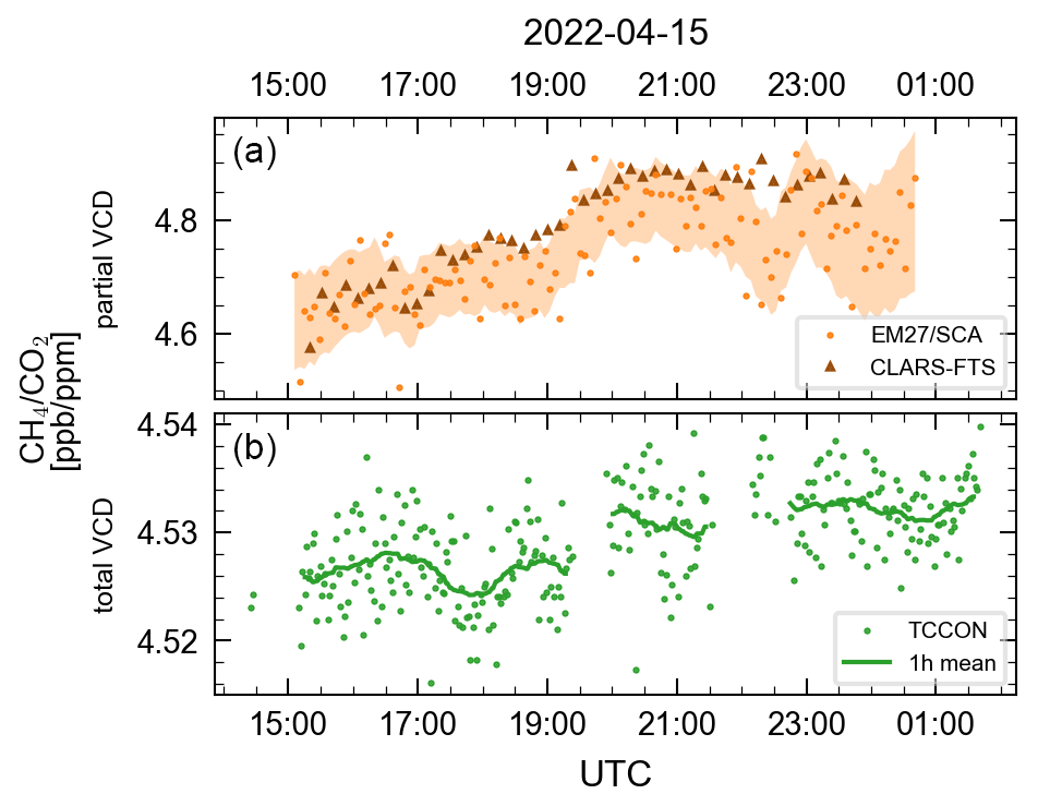
Figure A2 ${\mathrm{CH}}_{\mathrm{4}}/{\mathrm{CO}}_{\mathrm{2}}$ ratio between partial VCD below instrument level (a, as in Fig. 15) measured with EM27/SCA (orange dots) and CLARS-FTS (orange triangles), as well as total VCD measured by TCCON at CalTech, Pasadena (b, Wennberg et al., 2022).