the Creative Commons Attribution 4.0 License.
the Creative Commons Attribution 4.0 License.
 | 07 Nov 2023
GNSS radio occultation excess-phase processing for climate applications including uncertainty estimation
Josef Innerkofler
Gottfried Kirchengast
Marc Schwärz
Christian Marquardt
Yago Andres
Earth observation from space provides a highly valuable basis for atmospheric and climate science, in particular also through climate benchmark data from suitable remote sensing techniques. Measurements by global navigation satellite system (GNSS) radio occultation (RO) qualify to produce such benchmark data records as they globally provide accurate and long-term stable datasets for essential climate variables (ECVs) such as temperature. This requires a rigorous processing of the raw RO measurements to ECVs, with narrow uncertainties. In order to fully exploit this potential, Wegener Center's Reference Occultation Processing System (rOPS) Level 1a (L1a) processing subsystem includes uncertainty estimation in both precise orbit determination (POD) and excess-phase profile derivation.
Here we introduce the new rOPS L1a excess-phase processing, the first step in the RO profiles retrieval down to atmospheric profiles, which extracts the atmospheric excess phase from raw SI-traceable RO measurements. This excess-phase processing, for itself algorithmically concise, includes integrated quality control and uncertainty estimation, requiring a complex framework of various subsystems that we first introduce before describing the implementation of the core algorithms. The quality control and uncertainty estimation, computed per RO event, are supported by reliable forward-modeled excess-phase profiles based on the POD orbit arcs and collocated short-range forecast profiles of the European Centre for Medium-Range Weather Forecasts (ECMWF) Reanalysis (ERA5). The quality control removes or alternatively flags excess-phase profiles of insufficient or degraded quality. The uncertainty estimation accounts both for relevant random- and systematic-uncertainty components, and the resulting (total) uncertainty profiles serve as a starting point for the subsequent uncertainty propagation through the retrieval processing chain down to the atmospheric ECV profiles.
We also evaluated the quality and reliability of the resulting excess-phase profiles based on Metop-A/B/C (Meteorological Operational) RO datasets for three 3-month periods in 2008, 2013, and 2020 by way of a sensitivity analysis for three representative atmospheric layers (tropo-, strato-, mesosphere), investigating consistency with ERA5-derived profiles, influences of different orbit and clock inputs, and consistency across the different Metop satellites. These consistencies range from centimeter to submillimeter levels, indicating that the new processing can provide highly accurate and robust excess-phase profiles. Furthermore, cross-evaluation and intercomparison with excess-phase data from the established data providers EUMETSAT (European Organisation for the Exploitation of Meteorological Satellites) and UCAR (University Corporation for Atmospheric Research) revealed subtle discrepancies but overall very close agreement, with larger differences compared to UCAR in the boundary layer. The new rOPS L1a processing can hence be considered capable of producing reliable long-term data records including uncertainty estimation for the benefit of climate applications.
- Article
(6515 KB) - Full-text XML
- BibTeX
- EndNote


Satellite-based remote sensing observations of the atmosphere, throughout the troposphere and stratosphere, constitute an important backbone for contemporary atmospheric and climate science. With global warming ongoing and its worldwide environmental and socioeconomic implications, improvement in the observational foundation of Earth's climate system has become more important than ever (IPCC, 2021). The Global Climate Observing System (GCOS) therefore aims for the establishment and preservation of climate benchmark data records for the detection, projection, and attribution of changes in the climate system as essential (GCOS, 2021).
By observing essential climate variables (ECVs) (National Research Council, 2007; GCOS, 2021; Bojinski et al., 2014), the global navigation satellite system (GNSS) radio occultation (RO) measurements (e.g., Kursinski et al., 1996; Syndergaard, 1999; Hajj et al., 2002) qualify to provide benchmark data records, as they provide accurate and precise monitoring of ECVs, such as temperature and pressure over the troposphere and stratosphere, and tropospheric water vapor, with global coverage, long-term stability, and essentially all-weather capability (Anthes, 2011; Steiner et al., 2011, 2020).
During an occultation measurement, signals emitted by a GNSS satellite scan the atmosphere in limb-sounding geometry and arrive with a time delay at the receiving RO satellite in low Earth orbit (LEO), which occurs due to the signal's refraction in Earth's atmosphere. A vertical setting or rising occultation event is observed depending on whether the GNSS transmitter satellite sets or rises behind Earth's horizon, from the viewpoint of the rapidly moving LEO receiver satellite.
The raw phase change measurements, obtained by a GNSS receiver aboard the LEO satellite, fundamentally can be traced to the SI seconds, a requirement for RO measurements to serve as a fundamental climate data record (FCDR) (GCOS, 2021). This is ensured by atomic clocks aboard the GNSS satellites, which are linked to a ground-based atomic clock network for monitoring and correction of the space-based clocks. In order to maintain traceability of the less stable oscillators of the LEO satellite, the clock bias is estimated along with the position and velocity of the satellite within the precise orbit determination (POD) process (Montenbruck et al., 2008; Innerkofler et al., 2020). This allows for accurate georeferencing of the measurements in order to isolate the phase delay induced by the atmosphere. This so-called excess phase serves as a key FCDR variable available from the RO measurements. Within the RO retrieval, this FCDR can be processed further to vertical atmospheric profiles of bending angle and refractivity, as well as subsequently to ECVs, namely temperature, pressure, and tropospheric water vapor.
The assessment of the quality and uncertainty in RO data, caused by measurement and retrieval errors, is also affected by the use of external data that facilitate the retrieval (Wee and Kuo, 2015). The inclusion of auxiliary information in the retrieval and its influence advances with each step of the retrieval and hence partially degrades the fundamental SI traceability of the measurements. Evaluation of basic (low-level) RO data, in particular the excess-phase data record, benefits from very little influence of external data in its determination and therefore offers the possibility of obtaining highly accurate FCDRs.
For this reason the RO processing at the Wegener Center for Climate and Global Change (WEGC) underwent a substantial revision with the decisive change to start processing from raw measurement data and to independently perform POD of the LEO receiver satellites (Innerkofler et al., 2020). Prior to those changes, OPSv5.6 (Angerer et al., 2017), the former WEGC processing system, started with the supply of excess-phase data along with already interpolated orbit and clock data from the COSMIC (Constellation Observing System for Meteorology Ionosphere and Climate) Data Analysis and Archive Center (CDAAC). The current Reference Occultation Processing System (rOPS) (Kirchengast et al., 2016, 2018) now aims to process raw RO phase measurements into ECVs in a way which is SI-traceable to the universal time standard and which includes rigorous uncertainty propagation. This climate quality rOPS comprises the occultation data processing (ODP) from raw RO measurement data (Level 0) to excess phase (Level 1a), atmospheric bending angles (Level 1b), refractivity and dry-air profiles (Level 2a), and finally thermodynamic ECV profiles, as outlined in Fig. 1 (red box). As a basis for supporting ODP, the daily system modeling (DSM; green box) for observation geometry and atmospheric-background modeling and the event system modeling (ESM; orange box) for RO event geometry and environment modeling, as well as the simulation of RO profiles, were added.
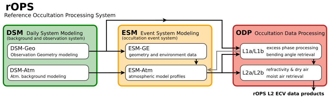
Figure 1General schematic overview of parts of WEGC's rOPS relevant to this study, comprising the daily system modeling (DSM; green), the event system modeling (ESM; orange), and the occultation data processing (ODP; red). The latter outlines the main Level 1 and Level 2 retrieval steps (L1a to L1b) from the excess phase to ECVs.
Within this study the new rOPS implementation of Level 1a excess-phase processing within rOPS is introduced, closing the gap between the calculation of precise orbit positions, velocities, and clock estimates (Innerkofler et al., 2020); the retrieval of bending angles (Schwarz et al., 2018); and, subsequently, refractivity and atmospheric profiles (Schwarz et al., 2017; Schwarz, 2018; Li et al., 2019). This includes the uncertainty estimation at the excess-phase level provided by rOPS for each individual RO event.
The random- and systematic-uncertainty estimates at the excess-phase level are then propagated through the entire ODP retrieval chain in order to provide the final ECVs with their associated uncertainties. Additionally, the uncertainties quantified are employed in part of the retrieval operators of rOPS to improve the derivation of variables (e.g., ionosphere correction, statistical optimization, moist-air retrieval). For details on the uncertainty propagation along this chain, starting from the estimates at excess-phase level, see Schwarz et al. (2018, 2017), Schwarz (2018), and Li et al. (2019).
Quality assessment of the algorithms is carried out based on RO data from the EUMETSAT (European Organisation for the Exploitation of Meteorological Satellites) Polar System (EPS) Meteorological Operational (Metop) satellite series (Luntama et al., 2008). Metop satellites provide a stable data record of RO measurements over more than a decade, which is routinely processed by two renowned processing centers: EUMETSAT as the operator of the mission (von Engeln et al., 2009) and CDAAC as an independent party (Schreiner et al., 2011). Simulated profiles extracted from European Centre for Medium-Range Weather Forecasts (ECMWF) ERA5 data (Hersbach et al., 2020) support this evaluation, which is subdivided into sensitivity, statistical, and uncertainty analysis (Sect. 4).
The Metop satellite series consists of three flight models, Metop-A/B/C, which were launched into orbit sequentially in time (Metop-A: 19 October 2006, Metop-B: 17 September 2012, Metop-C: 7 November 2018). All three satellites are equipped on board with the GNSS Receiver for Atmospheric Sounding (GRAS) RO instrument, developed by Saab Ericsson Space (SAAB, 2004; Klaes et al., 2007; Loiselet et al., 2000). Metop-A was then decommissioned by November 2021 (https://www.eumetsat.int/plans-metop-end-life, last access: 29 September 2023), while Metop-B and Metop-C are still in orbit and operational. The GRAS instrument provides dual-frequency navigation and occultation tracking at 12×3 channels for L1 C/A (coarse/acquisition) and L1/L2 P(Y) code. Besides a zenith-looking antenna providing navigation tracking data for POD, two high-gain antennas looking in the flight velocity and anti-velocity direction share 4 out of the 12 channels for recording setting and rising occultations, respectively. GRAS supports closed-loop (50 Hz) and open-loop (1 kHz) measurements (Bonnedal et al., 2010). RO data from EPS are limited to GPS observations, while EPS-SG (Second Generation) will be capable of tracking GPS, Galileo, and BeiDou signals (https://www.eumetsat.int/eps-sg-radio-occultation, last access: 29 September 2023). Hence, the scope of the new algorithm's evaluation in this study focuses on GPS RO data.
Following this introduction, in Sect. 2, the processing setup is described, the input data and their sources are summarized (Sect. 2.1), and the POD and background data modeling are introduced (Sect. 2.2). Subsequently, the excess-phase processing and algorithmic description are provided (Sect. 3.1), complemented by a description of the quality control and estimation of measurement uncertainties (Sect. 3.2). The results are presented and discussed in Sect. 4, before ending with a conclusion section (Sect. 5).
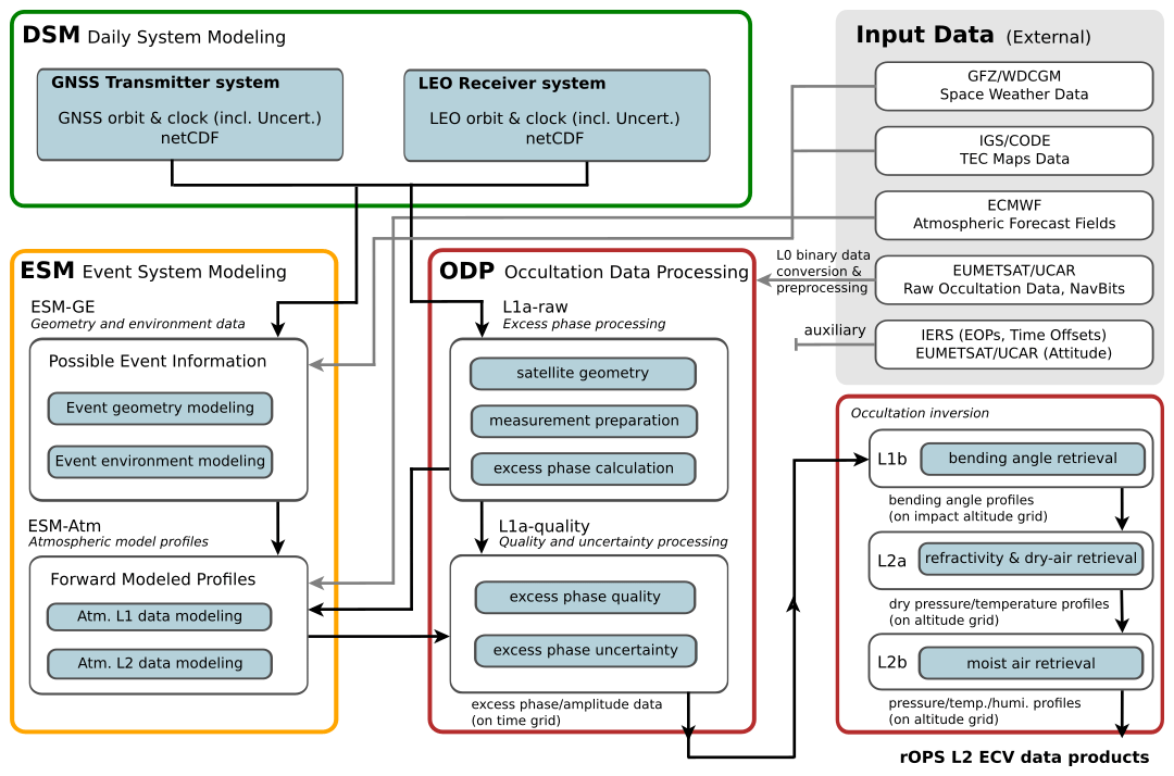
Figure 2Schematic overview of parts of WEGC's rOPS relevant to this study, comprising the daily system modeling (DSM; green), the event system modeling (ESM; orange), and the occultation data processing (ODP; red). Main details of subsystems are identified, with a focus on the ODP L1a processor, together with the major input data sources and output flow towards the L1b and L2 (L2a, L2b) retrieval chain from the excess phase to ECVs. GFZ: German Research Centre for Geosciences. WDCGM: World Data Center for Geomagnetism (Kyoto). IGS: International GNSS Service. CODE: Center for Orbit Determination in Europe. ECMWF: European Centre for Medium-Range Weather Forecasts. EUMETSAT: European Organisation for the Exploitation of Meteorological Satellites. UCAR: University Corporation for Atmospheric Research. IERS: International Earth Rotation and Reference Systems Service. EOPs: Earth orientation parameters.
Processing raw RO measurements to atmospheric excess-phase profiles, also termed Level 1a (L1a) processing, follows a basic algorithmic sequence sometimes also referred to as “calibration” of the measurements (Hajj et al., 2002). In practice, the inclusion of rigorous quality control, uncertainty estimation, and proper data preparation for the subsequent Level 1b (L1b) bending-angle retrieval algorithm make this L1a processing a fairly complex task. Within rOPS, the excess-phase processing is divided into two parts: (1) the derivation of the raw excess phase (the main calibration algorithm) and (2) the quality control and uncertainty estimation of the derived excess-phase profiles. Along with these two subprocesses, a series of steps, involving ESM-GE and ESM-Atm (cf. Fig. 1), complement the excess-phase computation.
Figure 2 summarizes the relations and workflow between those rOPS subsystems most relevant to the L1a excess-phase processing. In a first step, external input data have to be acquired and prepared to satisfy the rOPS data interface. DSM supplies precise and accurate orbit and clock data of LEO receiver and GNSS transmitter satellites, including estimates of systematic and random uncertainty. Subsequently, the ESM-GE models reference locations of all possible RO events and provides additional information on the geometry and environment, while the raw excess-phase profile processing delivers vertical profiles of measured RO data. With the event information and the raw L1a data, atmospheric excess-phase model profiles can be provided by ESM-Atm. These model profiles are then used for the L1a quality control and uncertainty estimation, yielding “final” quality-controlled excess-phase profiles, which serve as input for the ODP L1b retrieval processing. In the following, we take a closer look at each of these steps relevant to the L1a processing after summarizing the relevant input data.
2.1 Input data preparation
The RO data processing in general and, more specifically to this study, the WEGC ODP L1a excess-phase data processing rely on various input data sources. Besides the main observational data measured by the satellite's occultation antenna(s), space weather data, atmospheric reanalysis and forecast data, satellite antenna specifications, GNSS navigation bit data, and auxiliary data comprising Earth orientation data and time offsets are also necessary input data for RO excess-phase processing and its supporting ESM system. Table 1 provides a concise overview of these external data sources used for the L1a processing within rOPS and is followed by a description of the application of these data.
Hernández-Pajares et al. (2009)Matzka et al. (2021)Tapping (2013)ECMWF (2019)Hersbach et al. (2023)Rebischung and Schmid (2016)EUMETSAT (2016)EUMETSAT (2018)Table 1External input data used by the different subsystems of the rOPS ODP L1a processing system. Data are provided by the Crustal Dynamics Data Information System (CDDIS), German Research Centre for Geosciences (GFZ), Geomagnetic Laboratory (GEOLAB) of Natural Resources Canada, ECMWF, International GNSS Service (IGS), EUMETSAT, and International Earth Rotation and Reference Systems Service (IERS). For details on the specific data types, see the text. n/a: not applicable.
In this study we used three multi-month time periods as the basis for the assessment, each comprising 3 months: July to September 2008 (Metop-A; 2008-JAS), July to September 2013 (Metop-A/B; 2013-JAS), and December 2019 to February 2020 (Metop-A/B/C; 2020-DJF). These are representative of different solar cycle and summer/winter conditions over more than a decade from 2008 to 2020. As a cross-check, we also investigated data in the main season of equatorial plasma bubbles (September 2013 to March 2014), which involves particularly challenging geophysical conditions, but found no appreciable differences in comparison to the three time periods chosen. Data availability of the respective study periods is limited by the different launch dates of Metop satellites A, B, and C (cf. Sect. 1).
Compared to other RO receivers, the GRAS receiver on board the Metop satellites delivers raw-level measurement data in the form of chunks of numerically controlled oscillator (NCO) time-tagged phase as well as in-phase and quadrature (I/Q) components, instead of already connected phase and amplitude as a function of time (SAAB, 2004; Schreiner et al., 2011). Since the computation of these variables is time intensive and some data distribution limitations for original Level 0 data by EUMETSAT do apply, WEGC decided to reconstruct the raw variables from the EUMETSAT L1a data (EUMETSAT, 2016). This includes reconstruction of the raw measurement time stamps and undifferencing of the NCO phase. It was validated against processing based on EUMETSAT Level 0 data that such correctly performed raw-level measurement reconstruction does not show any non-negligible differences compared to the original data. We note that CDAAC developed their own phase and amplitude calculation for GRAS data, which also shows good agreement with data generated by EUMETSAT (Schreiner et al., 2011).
For evaluation of the calculated atmospheric excess-phase profiles, inter alia also of the proper implementation of the rOPS ODP L1a processing, a careful intercomparison with independently calculated profiles is indispensable. In this study publicly available excess-phase profiles from EUMETSAT (https://eoportal.eumetsat.int, last access: 29 September 2023; 2008-JAS and 2013-JAS: https://doi.org/10.15770/EUM_SEC_CLM_0029 (EUMETSAT, 2020), processor: Yaros 1.4; 2020-DJF: operational, processor: GRAS-4.6.2) and CDAAC (Metop-A: https://doi.org/10.5065/789w-m137 (CDAAC, 2023a), version: 2016.0120; Metop-B: https://doi.org/10.5065/1k0w-2272 (CDAAC, 2023b), version: 2016.0120; Metop-C: https://doi.org/10.5065/p8es-mc74 (CDAAC, 2023c), version: 2019.2580) have been used for such intercomparison (Sect. 4.2). Additionally, forward-modeled profiles computed from ERA5 reanalysis data (Hersbach et al., 2023) served as a reference for a sensitivity analysis for the excess-phase profiles calculated with rOPS (Sect. 4.1.1).
Reanalysis data are widely used in atmospheric sciences applications and also serve as an integral component in WEGC's rOPS system. The reference dataset used in this study is the ERA5 reanalysis dataset, computed with the Integrated Forecasting System (IFS) of the ECMWF (ECMWF, 2016, 2019; Hersbach et al., 2019, 2020). Within rOPS, ERA5 short-range forecast data are used for the provision of model and background profiles in order to facilitate the ODP retrieval and to derive quality measures and support estimation of the uncertainty in the observed profiles at each step of the retrieval, while the ERA5 analysis data are used for the provision of reference profiles in part of the sensitivity analysis of the RO retrieval.
The employed short-range forecast is essentially a pure model state carrying no direct information from assimilated observational data. This is an important aspect in order to keep the final rOPS ECVs uncorrelated with the evaluation (analysis) dataset, given that RO data are assimilated into ECMWF's (re)analyses as of late 2006 (Healy, 2007; Schmidt et al., 2008; Hersbach et al., 2020). Although the assimilation of RO data has an influence on the ERA5 analysis data, we consider this analysis suitable for supporting the task of evaluation of the quality and robustness of the implemented excess-phase processing in this study. We note that for the actual validation of data, which is not the focus here, further independent datasets should be used. With a horizontal resolution of about 30 km, with 137 vertical levels from the surface up to about 80 km, the ERA5 reanalysis data suit the RO measurement characteristics well. The interpolation strategy to produce collocated model, background, and reference profiles is summarized in Sect. 2.2.3.
For the ESM-GE processing, ionosphere and space weather information are incorporated to complement the environment information for each RO event. These data comprise total electron content (TEC) maps, Kp indices describing disturbances of Earth's magnetic field, and solar flux data measuring the radio emission from the Sun at a wavelength of 10.7 cm as a proxy for solar activity. These can support quality evaluation and, in particular, serve as an input for higher-order ionospheric correction in L1b processing (Danzer et al., 2020, 2021; Liu et al., 2020). In addition, GNSS and LEO antenna offset information is used to accurately model the event locations in ESM-GE and to correct the location of the observations in ODP L1a. For the GNSS, these data are provided by the International GNSS Service (IGS) using the antenna exchange format (ANTEX; https://files.igs.org/pub/data/format/antex14.txt, last access: 29 September 2023).
For the LEO receiver satellites, different sources need to be exploited depending on the RO mission and satellite data provider. At WEGC all relevant LEO antenna information is merged in a custom receiver antenna file, using the ANTEX format as well. GNSS navigation bit data for measurement signal demodulation are obtained from EUMETSAT (EUMETSAT, 2018). Variable Earth geodetic data, such as Earth orientation parameters (EOPs), leap seconds, and time offsets, serve as general input in support of coordinate and time transformations performed as part of the rOPS L1a processing.
2.2 Daily and event-based system modeling
The system modeling part of rOPS, in preparation for the ODP core system, consists of two main components: (1) DSM, the daily system modeling of the observation system geometry and preparation of atmospheric-background fields, and (2) ESM, the occultation event modeling of geometry and environment modeling and derivation of corresponding atmospheric-model profiles (Fig. 2).
2.2.1 Observation geometry modeling
Accurate and precise knowledge of the location and time of GNSS signal transmission and reception is fundamental to RO processing and the subsequent derivation of highly accurate and long-term stable ECVs. For this reason, a novel multi-system setup for POD was introduced by Innerkofler et al. (2020) that builds on independent orbit solutions from three different processing runs for each day. Embedded in the DSM observation geometry modeling of rOPS, the system also provides attributed measures for quality and estimated uncertainties, in order to enable long-term stable and highly consistent LEO orbit processing and analysis.
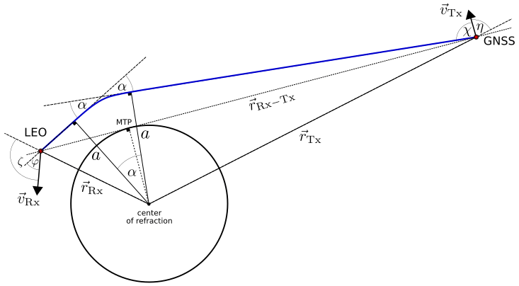
Figure 3Occultation event geometry, defining important location and angular variables of an RO event. Adapted from Pirscher (2010). The schematic depicts the occultation event at the time when the straight-line connection between GNSS and the LEO satellite is tangent to Earth's ellipsoidal and defines the mean tangent point (MTP) in this way.
Within DSM-Geo, the LEO POD of RO receiver satellites is performed in parallel by employing the two independent software packages of Bernese v5.2 (Dach et al., 2015) and NAPEOS v3.3.1 (NAvigation Package for Earth Observation Satellites) (Springer, 2009). The calculations are based on GNSS pseudorange and carrier phase measurements obtained by the RO satellite's zenith antenna and GNSS orbit and clock data products from the Center for Orbit Determination in Europe (CODE). One additional orbit solution is derived with transmitter orbit and clock data from the International GNSS Service (IGS) using Bernese. This POD setup enables mutual consistency checks of the calculated orbit solutions and is used for monitoring the quality of the “primary” orbit solution (the one derived with Bernese–CODE used for further RO processing) as well as for position and velocity uncertainty estimation, including estimated systematic and random uncertainties. In general, the combined 3D-estimated position and velocity uncertainties for the Metop satellite series account for around 1.9 cm and 0.02 mm s−1 (random) and 5.0 cm and 0.05 mm s−1 (systematic), respectively. For more details on this rOPS POD processing, the reader is referred to Innerkofler et al. (2020).
The additional uncertainty output produced by DSM-Geo exceeds the limitation of the well-established format definitions used for the exchange of orbit data, e.g., SP3 (Standard Product 3; https://files.igs.org/pub/data/format/sp3c.txt, last access: 29 September 2023). We therefore store the final output data of the POD in a specially designed netCDF file that contains orbit and clock data for each daily 24 h orbit arc per satellite. In total this results nominally in 32 GPS transmitter and 1 RO receiver satellite file per day. The content comprises the center-of-mass (COM) satellite positions and velocities in an Earth-centered, Earth-fixed (ECEF) coordinate system as well as satellite clock biases. Adequate for the intended purpose of RO processing (confirmed by comprehensive sensitivity checks), the GNSS orbit data are stored with a sampling rate of 15 min, whereas the clock bias data and LEO orbit data are stored at a sampling rate of 30 s. All these daily orbit arc data are stored together with their estimated random and systematic uncertainty.
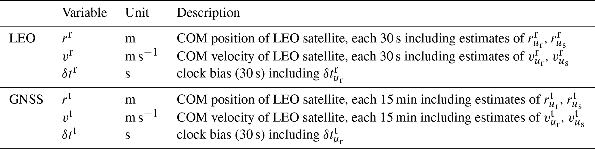
Table 2 provides an overview of the core variables supplied by the DSM-Geo POD processing, which subsequently serve as input for the ODP L1a processing. For the excess-phase processing these data need to be aligned in time (interpolation of RO measurement time stamps and correction of clock biases) and location (application of RO antenna offsets). The preparation and necessary steps for this processing are discussed further in Sect. 3.1.
Table 2Orbit and clock data output from the rOPS POD processing, including the associated sampling rates and corresponding estimates of random (ur) and systematic uncertainty (us).
2.2.2 Event system modeling
Provided the positions and velocities of the transmitter and receiver satellites, calculated by DSM-Geo, a reference event location of an occultation is determined in rOPS by geometrical constraints only, independent of any atmospheric state or RO measurement data. The selected reference location of an event is defined on Earth's ellipsoidal surface at the time when the straight-line connection between receiver and transmitter satellite is tangent to Earth's surface (WGS-84 EGM2008; World Geodetic System, Earth Gravitational Model; cf. Fig. 3 for measurement geometry). This uniquely defined point in space and time, also referred to as the mean tangent point of the RO event, is determined after the GNSS orbit is interpolated to the 30 s sampled LEO orbit time stamps (and locally using fine interpolation for accurately determining the point). For compact identification, each event is uniquely encoded using a 64-bit integer representation compiled from the mean event time, transmitter system, and transmitting-satellite identifier, as well as the receiver identifier.
The event geometry modeling is complemented by the event environment modeling comprising surface and atmosphere data, as well as ionosphere and space weather information extracted for each reference location. Apart from the mean tangent point, which per definition is at a straight-line tangent height (SLTH) of 0 km, the same information can be additionally retrieved for any other non-zero SLTH. In rOPS this is done additionally at an SLTH of 90, 80, 70, 60, and −250 km, respectively. Extracted parameters and variables at these auxiliary locations visited during the RO event is valuable for contextual grouping of events, event distribution analyses, and ionosphere/space weather sensitivity analyses and is also needed in the subsequent ODP processing, e.g., as part of higher-ionospheric correction (Danzer et al., 2021; Liu et al., 2020).
The mean tangent point location derived in this way has been proven to be very adequate and corresponds to real RO event tangent point trajectory locations near the tropopause (Foelsche et al., 2011). This offers the advantage that purely geometrical analyses, like those for geographic RO event distributions, can be done independent of RO data, and it enables rigorous location consistency of forward modeling (simulating RO profiles) and retrievals (analyzing observed profiles) for each and for all individual events. Figure 4 illustrates the global RO event distribution for Metop-A/B on 1 July 2013. In principle the number of modeled events exceeds the number of observed events. The calculated data of ESM-GE are provided as a dedicated output file of rOPS and then are further used by the subsequent ESM subsystems and the ODP L1a processing.
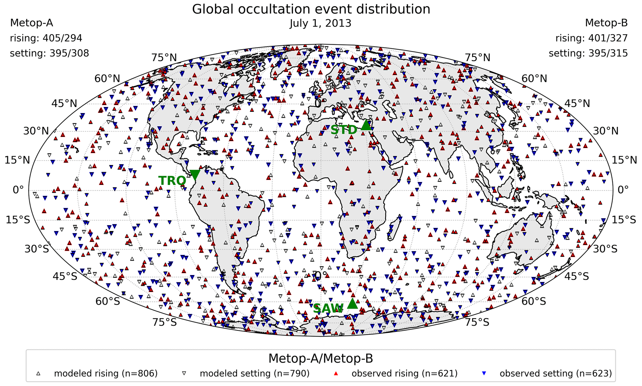
Figure 4Global distribution of Metop-A/B RO events on 1 July 2013. Setting events (upside-down triangles) and rising events (upright triangles) are separately identified, and the number of modeled/processed events is noted as part of the legend information. Three example events used for illustrating the subsequent description and results are separately identified (large green triangles) as well, with more information on them summarized in Table 3).
2.2.3 Atmospheric-model profiles
With knowledge of the simulated but realistic event location of the measurements from ESM-GE, corresponding atmospheric profiles can be forward-modeled upward along the ODP processing chain from Level 2 to Level 1. Figure 5 illustrates the forward-modeled results, extracted from ERA5 data at the respective locations, for the three example events (see Fig. 4 and Table 3), for refractivity (N), bending angle (α), and excess phase (L), respectively, as well as the difference profiles between the forward-modeled and related observed excess-phase data. These example profiles serve to represent standard (STD), tropical (TRO), and sub-arctic winter (SAW) conditions. Given the simulated event locations, it is ensured that for each observed RO event, a corresponding consistent set of forward-modeled profiles is made available at each step from refractivity to the excess phase.
Table 3Selected Metop-A RO example events, representing standard (STD), tropical (TRO), and sub-arctic winter (SAW) conditions.
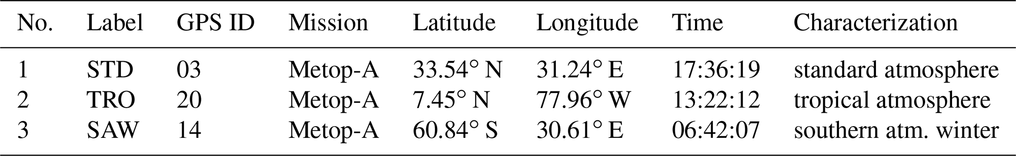
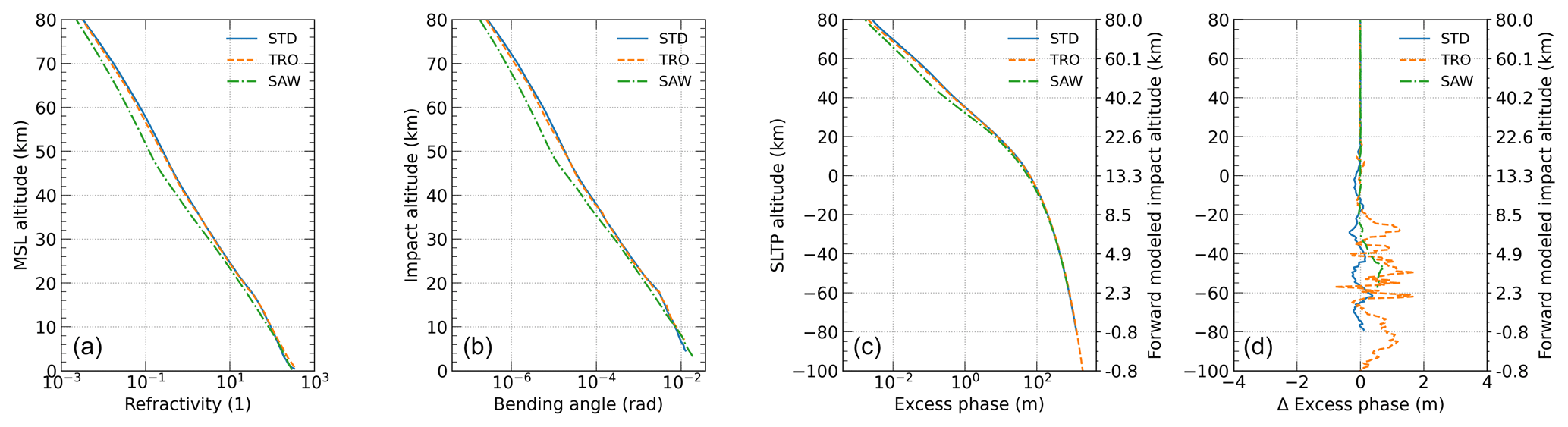
Figure 5(a–c) Forward-modeled example profiles from (a) refractivity to (b) the bending angle and (c) the excess phase, respectively, and (d) the difference between modeled and observed excess phase. Results for all three example events defined in Table 3 are shown. MSL: mean sea level. SLTP: straight-line tangent point.
The ERA5 reanalysis fields, introduced in Sect. 2.1 above, globally provide temperature, pressure, and water vapor information at any desired location and time of interest. Hence, starting from ERA5 fields, atmospheric profiles of these variables are extracted by interpolation in time and space to the RO event location (mean tangent point location, extracting vertical profiles at these locations). Since the ERA5 fields are used in a 6-hourly resolved form, the closest time layer happens to always be within 3 h of the occurrence of the mean RO event time, a time difference which is sufficient to model the semi-diurnal cycle (Scherllin-Pirscher et al., 2011b, a). Horizontal interpolation is performed by using a four-point cubic-polynomial interpolation technique (for a detailed description, see Appendix A.3 of Lackner, 2010). For vertical interpolation of temperature T, pressure ln(p), and specific humidity q, several interpolation methods were compared (linear, cubic spline, and Savitzky–Golay filter). Based on this, those providing the most robust fit through the nodes of the ECMWF altitude levels were selected. As a result, the vertical interpolation to the fixed-altitude grid z is performed for T and ln(p) using a natural cubic-spline interpolation, while q profiles are interpolated linearly.
Refractivity profiles are then derived, based on the interpolated variables, employing the ionosphere-free first-order relationship (Smith and Weintraub, 1953; Kursinski et al., 1997). Given the refractivity profile as a function of the fixed vertical grid N(z), Level 1 profiles of bending angle α, Doppler shift D, and excess phase L can be calculated.
In a first step impact altitude grid and impact parameter grid are computed consistently with altitude grid z, with geoid undulation UG and radius of curvature RC both at the occultation event location. Additionally log-refractive index profile and its gradient profile are calculated at the consistent grids.
Using the refractive index gradient profile the bending-angle profile α(az) is then derived using an inverse Abelian integral transformation (Fjeldbo and Eshleman, 1965; Fjeldbo et al., 1971), solving for all grid levels ai from a(ztop) to a(zbot). The actual calculation is performed using the implementation in rOPS (Syndergaard and Kirchengast, 2016) in combination with the baseband method (cf. Kirchengast et al., 2018). Subsequently, the bending-angle profile is mapped to a strict 50 Hz measurement grid including a vertical mapping from impact altitude α(a) to time α(t). This mapping requires knowledge of the orbit position of the transmitter (rTx) and receiver (rRx) satellites at the measurement time and demands an iterative numerical solution (Proschek et al., 2011).
The mapped bending angle α(t) is then used to calculate the Doppler shift, which can in turn be further integrated to the excess phase. Based on the occultation geometry (cf. Fig. 3) and the corresponding angles χ, η, φ, and ζ, as well as the position and velocity of the receiver (rRx, vRx) and transmitter (rTx, vTx) satellites and their distance to each other drRxTx, the Doppler shift can be calculated as follows:
with
and
Modeled Doppler shift D(ti) is limited to the proportion of the entire Doppler shift, which is induced by the atmosphere, while those parts which come from the movement of the satellites relative to each other are not considered.
Finally, modeled excess phase L(ti) can be calculated as a function of time by using the relation with the previously calculated Doppler shift D(ti):
To integrate the excess-phase change (or Doppler shift), in order to obtain the excess-phase path, we apply Simpson's rule for the numerical integration of Eq. (3). The integration starts at the top of the measurement, where D is very small and errors in the initialization almost vanish relative to contributions at lower-atmospheric levels. Scale height H multiplied by the bending angle α at the uppermost level serves as integration constant , which is considered an adequate approximation for the integration of the excess phase (Rieder and Kirchengast, 2001; Kirchengast et al., 2018).
3.1 Excess-phase processing
Numerous studies have described the RO retrieval chain in detail (e.g., Kursinski et al., 1997; Rieder and Kirchengast, 2001; Hajj et al., 2002; Kuo et al., 2004) and have shown the high accuracy of RO data, particularly in the upper-troposphere and lower-stratosphere region (e.g., Rocken et al., 1997; Gobiet et al., 2007; Ho et al., 2012; Steiner et al., 2020). More specifically, RO Level 1a processing data from raw occultation measurements and precise orbit and clock data of the transmitter and receiver satellites to the excess phase have been discussed in detail (e.g., Hajj et al., 2002; Beyerle et al., 2005; Schreiner et al., 2010; Bai et al., 2018), since accurate and precise excess-phase data are the indispensable basis for SI traceability and co-determine the quality of derived ECVs. Here the implementation of WEGC's new rOPS ODP L1a excess-phase processing is described, preceded by a short discussion of GNSS signal structure and signal-tracking modes.
3.1.1 GNSS observables
In principle, the concept of GNSS measurements relies on measurements of ranges between the transmitter and receiver which are derived from measured time (code pseudoranges) or phase differences (phase pseudoranges) relative to the transmitted electromagnetic signal. Since the measured ranges are affected by transmitter and receiver satellite clock errors, they are labeled pseudoranges. Also, more commonly simply referred to as code and (carrier) phase measurements, those observables constitute basic measurements made by GNSS receivers aboard RO satellites, where the latter (carrier phase) are more precise and therefore favored in RO processing. This is intrinsic to the chip length of the code modulated onto the carrier phase (e.g., GPS, coarse/acquisition (C/A) code: λ≈293 m; precision (P) code: λ≈29 m), which is accurate to 1 %–0.1 %, while carrier phase measurements of a typical GNSS wavelength (e.g., GPS, L1: λ≈0.19 m; L2: λ≈0.24 m) allow for millimeter precision (Teunissen and Montenbruck, 2017; Hofmann-Wellenhof et al., 2008).
The enhanced precision of the carrier phase measurements comes with the disadvantage of ambiguity of the measurement, since at the time of the initial signal acquisition the number of full carrier wave cycles (“integer cycles”) between the receiver and the transmitting satellite is not known. Although this is a problem for classical navigation and positioning applications, for atmospheric RO, interested in the relative change in the signal for vertical atmospheric profiling, it does not pose a problem (Teunissen and Montenbruck, 2017).
Phase measurements are generally performed using a phase-locked loop (PLL), where the receiver generates an internal replica of the GNSS signal, aligns it with the incoming carrier phase, and measures it while keeping track of the changes in full cycles and the fractional shift (I/Q). Within PLL tracking, the internally generated signal is adjusted using a feedback loop on the basis of previous measurements, which works fine with a sufficiently high signal-to-noise ratio (SNR) and weak atmospheric disturbances in the atmospheric regions above the lower troposphere. In the lower troposphere, however, the complicated structure of RO signals, caused by multipath propagation or even ducting in the moist lower troposphere, leads to a loss of lock or to biases in the measured signals as well as to late signal acquisitions for rising occultations that may miss the moist lower troposphere (Sokolovskiy, 2001; Sokolovskiy et al., 2006; Ao et al., 2009).
In order to overcome these issues, RO signals are measured using a delay-locked loop (DLL) when disturbed atmospheric conditions interfere with closed-loop (CL) tracking using a PLL. This OL-tracking (open-loop) mode is not supported with a feedback loop including the measured signal (and is therefore less prone to be affected by disturbed atmospheric conditions) but is model-aided based on orbit, receiver clock drift, and estimated Doppler shift and delay, deduced from a real-time navigation solution (e.g., Ao et al., 2009). This onboard computation of the OL model, including the prediction of the code pseudorange, is employed by the majority of GNSS RO receivers currently in space. Note that RO measurements performed using OL tracking need to be demodulated from GNSS navigation data in postprocessing (Sokolovskiy, 2001; Sokolovskiy et al., 2006).
The GRAS receiver, in contrast, continues C/A code tracking in OL mode and only uses an OL model for carrier phase tracking. This can lead to data gaps when the C/A code tracking loses lock caused by challenging tracking conditions in the lower troposphere (Schreiner et al., 2011). Therefore, in order not to degrade SI traceability, we restrict the processed data to the longest continuous CL and raw-sampling (RS) data segments, not allowing for any gaps between these two data segments. Another method to overcome the shortcomings of CL tracking in the lower troposphere is to use moderate wideband digital recording, a technique which features a sufficient bandwidth to capture the spectrum of the excess Doppler in the lower troposphere (Ao et al., 2009). For GRAS on board Metop (Bonnedal et al., 2010) this was realized by the implementation of the RS-tracking mode, scanning the GNSS signal with a frequency of 1 kHz (SAAB, 2004; Gorbunov et al., 2011; Zus et al., 2011). This bears the advantage that only geometric effects need to be modeled in the tracking loop, but at the same time data storage requirements increase significantly compared to 50 Hz OL tracking featuring narrowband digital recording (Sokolovskiy, 2001; Ao et al., 2009).
Independent of the tracking mode employed, the RO technique aims to extract atmospheric and ionospheric delays from the total measured phase. The measured phase between the GNSS transmitter and LEO receiver satellites, denoted with the superscript t and the subscript r, respectively, can be modeled for a given GNSS signal frequency, summing up the following terms as a function of signal reception time tr at the LEO satellite and transmission time tt at the GNSS satellite (Schreiner et al., 2010):
where (tr) denotes the total observed carrier phase in units of length, (tr,tt) denotes the geometrical distance between the transmitter and receiver satellites, δtr (tr) denotes the receiver clock error (or bias/offset), δtt (tt) denotes the transmitter clock bias (or offset), δtr,rel (tr) denotes the special relativistic effect on the receiver clock, (tt) denotes the special relativistic effect on the transmitter clock, (tr) denotes the ionospheric delay, (tr) denotes the neutral atmosphere delay, (tr,tt) denotes the general-relativistic gravitational delay, and denotes the integer phase ambiguity, with the signal wavelength λ, speed of light in a vacuum c, and ϵ of the phase noise and residual errors.
3.1.2 Atmospheric and ionospheric excess phase
For the purpose of remote sensing of Earth's atmosphere, the atmospheric influences, comprising effects of the neutral atmosphere and the ionosphere , need to be separated from the phase model as specified above. Thus, all terms in Eq. (4) apart from the neutral atmosphere delay and ionospheric delay need to be modeled or removed in order to isolate the atmospheric and ionospheric excess phase:
The ionospheric part can then later on be removed using a linear combination of the dual-frequency measurements (Schreiner et al., 2010) or more refined RO-tailored corrections at the bending-angle level (Vorob'ev and Krasil'nikova, 1994; Ladreiter and Kirchengast, 1996; Liu et al., 2013; Healy and Culverwell, 2015; Liu et al., 2020). As depicted in Fig. 6, the separation of the excess phase includes a series of corrections to the measurement geometry and the measured signal itself. In the following the necessary steps for the excess-phase calculation and the implementation in rOPS are discussed in more detail.
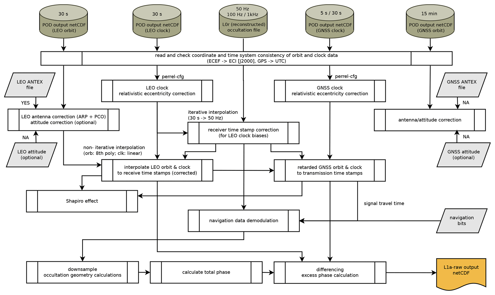
Figure 6rOPS ODP L1a excess-phase processing algorithm workflow. For description and explanations, see the text. NA: not applied.
3.1.3 Satellite geometry – orbit and clock corrections
As a first step of the ODP L1a excess-phase determination, the accurate space–time points of the signal's transmission and reception need to be determined. Therefore, the low-rate GNSS and LEO orbit data need to be corrected and then interpolated to the high-rate RO measurement time stamps. This process includes the removal of receiver and transmitter clock biases, relativistic corrections, the calculation of the signal travel time, proper coordinate transformation of the antenna offsets and addition to the satellite’s COM, and the calculation of the geometric distance between receiver and transmitter satellite antennas (see Fig. 6).
At the beginning of the ODP L1a processing, all the necessary input data (cf. Sect. 2.1) are read and checked for their consistency. Starting with precise orbit and clock data from ESM-Geo, the coordinate and time systems of the data are examined. The positions and velocities of the satellites are converted from an Earth-centered, Earth-fixed (ECEF) to an Earth-centered inertial (ECI) reference frame. That way, all calculations are independent of Earth's rotation correction (Sagnac effect; Ashby, 2004), which has to be taken into account when working in a rotating, Earth-fixed reference frame. More specifically, we use the J2000 coordinate system as a realization of the ECI reference frame for all calculations.
The atomic clocks aboard the GNSS satellites are considered stable over the short duration of an occultation event of approximately 1 to 2 min, with 1 s stability (Allan deviation) at a level of between 10−11 and 10−12, while more up-to-date clocks feature even higher accuracy (Griggs et al., 2015; Hauschild et al., 2013). In contrast to the GNSS satellites, the RO LEO missions do not carry atomic clocks on board; hence timing is in principle less accurate. However, among other RO missions, the Metop-A/B/C satellites use ultra-stable quartz oscillators that are likewise highly accurate over the short term of RO events. LEO clock errors δtr (bias estimates along time) are estimated along with the orbit determination process at WEGC, while GNSS clock bias estimates δtt are provided as part of the orbit data products by the CODE (or IGS) analysis center. The selection of a suitable differencing method, applied later in the excess-phase calculation (see Sect. 3.1.4), is dependent on the stability of the LEO clock.
Satellites and their clocks move with considerable speed in Earth's gravity field and orbit at fairly high altitudes above the surface, and hence effects of Einstein's theory of special and general relativity need to be taken into account. The reduced gravitational influence in orbit, compared to Earth's surface, causes a blue shift and satellite clocks to tick a little faster, whereas time dilation, induced by the motion of the satellites, reduces clock frequency (Ashby, 2003). At higher orbit altitude, such as for GNSS clocks, the former effect prevails. Therefore, these atomic clocks are intentionally slowed down prior to the GNSS satellite's launch by a certain clock frequency shift, in order to compensate for their time acceleration in orbit (Ashby, 2014; Mudrak et al., 2015). An additional periodically varying gravitational frequency shift and second-order Doppler shift, induced by the eccentricity of the satellite orbit, are modeled based on the LEO position rr and velocity vr at the signal reception time and the GNSS position rt and velocity vt at the signal transmission time, respectively (Kouba, 2015, 2004):
By convention, GNSS clock products provided by IGS and CODE analysis centers do not contain this so-called eccentricity correction (Kouba, 2015), and for this reason it needs to be applied to the transmitter clock in RO excess-phase processing. For LEO satellites, however, such a convention does not exist, and the correction might be handled differently in POD processing. At WEGC, Bernese (v5.2) by default does not explicitly model this correction, whereas we had to modify NAPEOS to align the processing strategy between the two POD software packages. In practice, if the effect is not explicitly modeled, it is absorbed in the POD clock error estimate and δtr,rel is set to 0. However, explicit modeling of the eccentricity correction of the LEO clock can reduce variability and therefore slightly enhance interpolation residuals.
In addition to the relativistic effects acting on the satellite clocks we model the far smaller gravitational time delay acting on the GNSS signals transmitted between the GNSS and LEO satellites as follows:
where G is the gravitational constant, ME is the mass of Earth, and rt and rr are the satellite and receiver radial position at signal transmission and reception times (Ashby, 2014; Mudrak et al., 2015). This effect is also referred to as the Shapiro time delay.
The GNSS and LEO orbits are provided with the satellite's mass center as a reference point and hence need to be corrected for the antenna offsets (from COM) in order to reflect the proper locations of the RO signal's transmission and reception. In general, those antenna offsets are composed by the geometric antenna reference point (ARP); the electromagnetic phase center offset (PCO) accounting for deviation from the geometric ARP; and, dependent on the signal's incoming direction, the phase center variation (PCV). As the PCV is a rather small effect, considering the short duration of an occultation event, it can be disregarded in RO processing (Hajj et al., 2002). The LEO RO antenna offsets (ARP and PCO) are applied using definitions provided in the so-called ANTEX format (cf. Sect. 2.1) and common coordinate transformation from the satellite body frame to ECI (EUMETSAT, 2005). Corrections for the changing orientation of the satellite in space and the deviation from nominal attitude during orbital revolution are not yet implemented in rOPS. However, although for missions with a stable orientation like Metop, this correction is small, it was found that not applying the correction introduces a small residual bias in bending-angle data (Alemany et al., 2022). Therefore, it is treated as a priority to include this correction in a future version of rOPS. On the GNSS transmitter side, neither GNSS antenna offsets nor their attitude is modeled, since they have a far smaller effect on RO processing than the LEO antenna offsets (Hunt et al., 2018).
After the correct handling of the relativistic eccentricity corrections and application of LEO antenna offsets, we can proceed and interpolate the LEO clock corrections, available at a low 30 s sampling rate, to the high-rate (50 Hz) RO measurement time stamps. This is done in an iterative procedure using a linear interpolation method until it converges at an empirically determined precision threshold. Once the corrected high-rate receive time is available, the LEO orbit and clock data from the POD-derived DSM-Geo orbit arcs are well interpolated to these time stamps, using an eighth-order polynomial Lagrange interpolation for satellite positions and velocities and a linear interpolation for its clock biases.
While the reception time of RO signals is recorded by the receiver and its biases are modeled and estimated, the signal transmission time of phase measurements needs to be reconstructed in order to allow for extraction of corresponding GNSS orbit and clock data. Assuming a straight-line propagation in a vacuum medium of the signal is considered sufficient to infer signal travel time τ, which elapsed during the signal's transmission at the GNSS satellite and the reception by RO receiver on the LEO satellite, with an iterative approach starting with τ0=0,
and therefore signal transmission time . Within the signal travel time calculation routine, the GNSS orbit positions are also updated and interpolated to tt. Once the iterative calculation of the signal transmission time converged, the GNSS velocity and clock data are interpolated the same way as was performed for the LEO satellite. Note that the retrieved geometric distance , required for the extraction of the RO excess phases, is a function of two time system variables tt and tr.
3.1.4 Measurement correction and preparation and differencing
At this point we have available all the correction terms necessary for the excess-phase calculation in Eq. (5): geometric distance between corrected GNSS and LEO satellites at signal receive time (tr), interpolated clock bias estimates δtt (tt) and δtr (tr), corresponding relativistic eccentricity correction terms δtr,rel (tr) and (tt), and relativistic Shapiro effect (tr). Effects not modeled, such as antenna phase wind-up (Bai et al., 2014, 2018), and residual errors are accounted for in error budget ϵ, which we will discuss in Sect. 3.2. However, depending on the RO receiver type, the raw measurements recorded in CL, OL, or RS tracking are also subject to corrections and preparatory steps before total phase (tr) can be used in the calculation: the navigation data demodulation, downsampling to a nominal measurement frequency (i.e., 50 Hz) of higher-sampled tropospheric measurements (e.g., Metop GRAS 1 kHz RS), and assembling of the total phase.
GNSS signals are modulated with a binary [0, π] navigation data message (NDM) providing useful information, such as ephemeris, clock, ionospheric, and service parameters, but at the same time introducing carrier phase flips to the signal. In CL tracking, these phase changes of π are corrected in real time at the RO receiver in orbit, whereas in lower-troposphere tracking (OL, RS) the NDM must be demodulated in postprocessing on the ground by either (Sokolovskiy et al., 2006) (1) the internal removal by detection of phase switches between adjacent samples or (2) the application of an externally provided NDM data stream (see Sect. 2.1; EUMETSAT, 2018). In general, as well as at WEGC, the latter strategy is preferred, in particular for climate application, because increasing disturbances in the lower troposphere can exceed the NDM-induced phase flips and introduce substantial retrieval errors if performing internal NDM removal (Sokolovskiy et al., 2009). Note that the previously calculated signal travel time τ is used to align the measurement data and the NDM bits at the signal transmission time, which are then used directly to revert the phase flips in the measured residual I/Q components.
Measurement data exceeding the 50 Hz sampling rate for RO CL measurements are downsampled to this nominal sampling frequency. Schreiner et al. (2011) investigated different downsampling target rates for Metop GRAS 1 kHz RS data and suggested using a sampling of 100 Hz for RO measurements in the lower troposphere, but also 50 Hz data lead to very similar results (Gorbunov et al., 2011). So far a sampling rate of 100 Hz has been realized for COSMIC-2 (Schreiner et al., 2020) and FengYun-3 (FY-3) GNOS (GNSS Occultation Sounder) (Bai et al., 2018). For GRAS RS data specifically, we calculate the arithmetic mean of 20 adjacent samples in order to obtain downsampled RO signal at 50 Hz. The SNR is then recalculated from the raw I/Q components with amplitude , while the NCO phase Lnco is interpolated linearly to 50 Hz.
With the corrected in-phase and quadrature I/Q signal components and the receiver model phase, the total measured phase can be constructed. First the ith sample of the residual phase in radians is calculated by for all four quadrants, before unwrapping the signal so that adjacent samples of the residual phase are always within ±π:
where ki is defined by minimization of . Finally, the total phase is obtained by , where division by 2π converts the residual phase from radians to cycles and λ denotes the wavelength of the GNSS signal in question.
With all terms available, we now can calculate excess phase following Eq. (5), representing a zero-differencing approach. This means that no clock differencing method is applied and the receiver clock bias estimates are employed directly in the differencing equation. This is the preferred option, introducing the lowest amount of noise in the processing, but is only practical for RO missions with a sufficiently stable LEO clock (ultra-stable quartz oscillators; e.g., Metop; GRACE, Gravity Recovery and Climate Experiment; FengYun-3). For other missions with less stable LEO clocks (e.g., CHAMP, Challenging Minisatellite Payload; COSMIC), the receiver clocks biases are removed by introducing a reference clock from a non-occulting GNSS satellite link in a so-called single-differencing approach (Schreiner et al., 2010; Beyerle et al., 2005; Bai et al., 2018). This alternative differencing is not applied in this study.
3.2 Quality control and uncertainty estimation
Following the calculation of excess-phase profiles as a function of time – including SLTP altitudes as an initial vertical-level variable – by the ODP L1a raw processor, the quality and uncertainty in these profiles are assessed in the ODP L1a quality processing. ESM-Atm provides modeled excess phases for each measured RO event, which serve as an important input to ODP L1a quality (cf. Fig. 2). Following the sequence we implemented, we will first discuss the quality assessment of the excess-phase profiles, including possible rejection, before addressing the associated uncertainty estimation.
3.2.1 Quality control
The rOPS L1a quality control (QC) process flags or (optionally) excludes unphysical or low-quality excess-phase profiles from further processing in order to provide a standardized input for the uncertainty estimation and to ensure the highest quality in the subsequent retrieval steps towards thermodynamic variables. If an event is not entirely rejected, specific QC flags are set (and written to a separate monitoring file) for data which are not passing the various quality checks or for which certain parts of the measurement are truncated at basically reliable top and bottom altitude levels. Key variables of the QC system are the observed excess-phase profiles and the independent forward-modeled excess-phase profiles as well as their delta profiles with suitable low- and high-pass filtering applied.
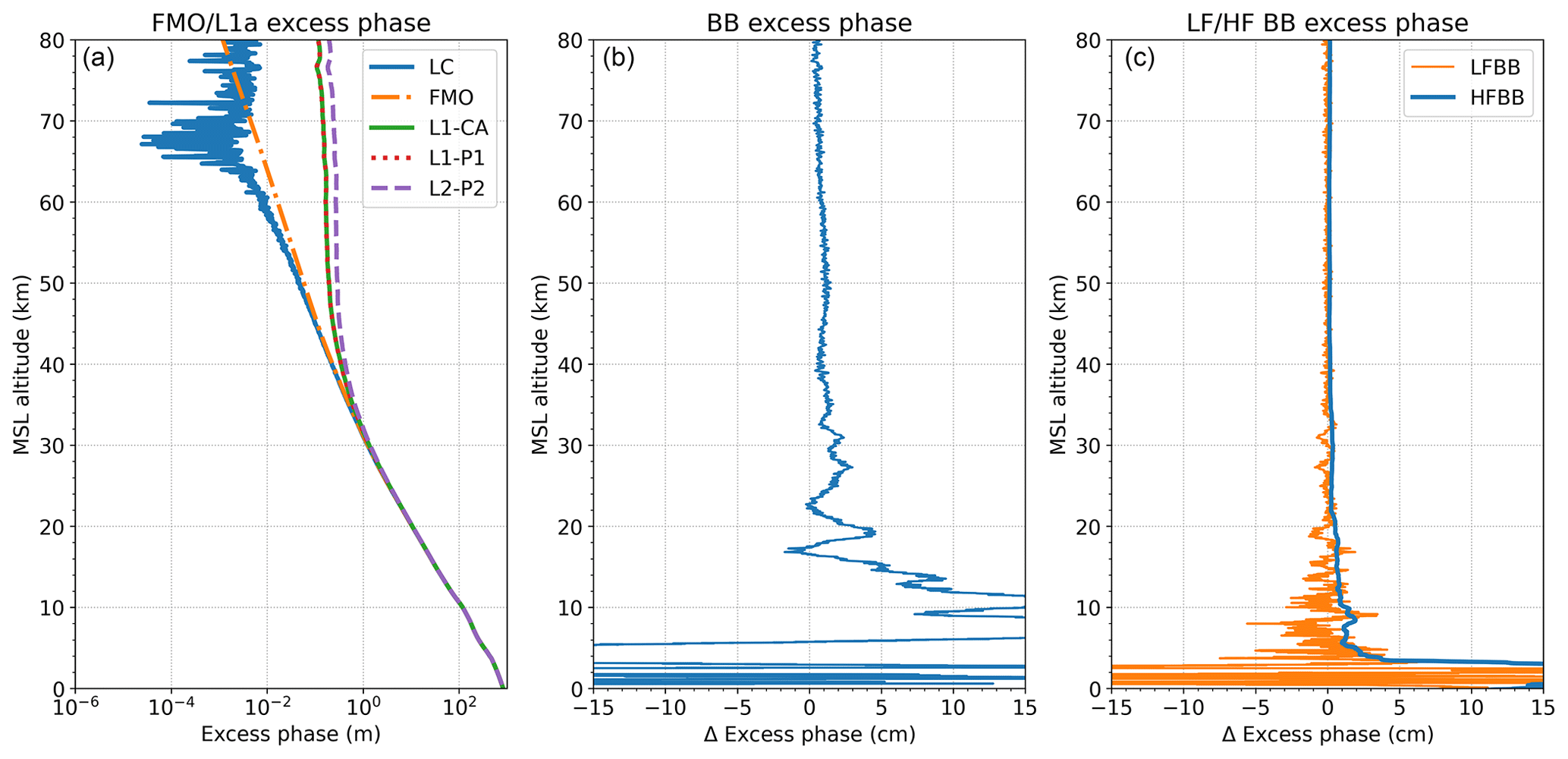
Figure 7(a) Illustration of forward-modeled (FMO), observed coarse/acquisition code (L1–CA), precise codes (L1–P1 and L2–P2), and linearly ionosphere-corrected (LC) excess-phase profiles, all as a function of (forward-modeled) MSL altitude. Additionally shown are (b) the derived baseband (BB) delta excess phase and (c) the low-pass-filtered (LF) BB and high-pass-filtered (HF) BB delta excess-phase profiles. These different phase profile examples are shown for an exemplary setting RO event from Metop-A (1 July 2008, 00:01 UTC; lat −72.3∘, long 37.6∘).
Central to the quality checks performed is the evaluation of the observed excess-phase data against the independent forward-modeled data. Since the modeled excess-phase profiles are free from ionospheric influences, we derive the ionosphere-corrected excess-phase profile by the classical first-order linear combination of the observed dual-frequency GNSS excess phases, e.g., for GPS (Schreiner et al., 2011),
with f1 and f2 being the GPS carrier frequencies of the corresponding L1 and L2 excess-phase profiles. Figure 7 (left) illustrates such profiles.
The signal strength and thus the penetration depth in the troposphere differs among the different GNSS signals involved in Eq. (10). Hence, the derived Lc profile is restricted to the altitude range covered by the shorter of the two signals. To overcome this limitation we artificially extend the shorter signal using a linear extrapolation downwards to match the reach of the stronger signal. This is realized by determination of the linear gradient of the difference profile of both signals over a sufficiently long altitude range (10 km) above the end of the shorter weak signal, with the lowest-allowed altitude of 15 km, to avoid the usage of data with a low SNR. The extrapolated part is then obtained by subtraction from the leading signal to obtain the extended weaker signal. The extended ionosphere-corrected excess-phase profile Lc in this form serves just as an auxiliary variable for the L1a QC. The ionospheric correction as part of RO retrieval is performed in a more advanced manner at the ODP L1b bending-angle level, including also higher-order correction (Danzer et al., 2021; Liu et al., 2020).
Within rOPS and specifically also for the ODP L1a quality control, the analysis and processing on delta profiles play a central role. Following the so-called baseband approach, with the subtraction of background model profile Lm (ESM-Atm) from retrieved profile L (ODP L1a), biases from the (near) exponentially varying RO profiles can be removed. This also leads to very small residual numerical errors in operators such as filters and derivatives: . Residual noise in the high-frequency domain of baseband excess phase δLBB can be suppressed by a low-pass filter, leading to a delta phase profile without noise and smaller variations, which better displays the large-scale effects of the atmosphere. We use a Blackman windowed sinc (BWS; Smith, 1999) low-pass filter FBWS with a cutoff frequency fc at 0.5 Hz. With a sampling rate of fs=50 Hz the suitable window size is data points, which corresponds to an effective filtering window size of 100 points or 2 s. For a more detailed description and discussion of advantages of a BWS filter over moving-average boxcar filters, see Schwarz et al. (2018, their Appendix 1.2). The low-pass-filtered baseband excess phase is then obtained as δLLFBB=FBWSδLBB. Subtraction of the low-pass-filtered baseband excess phase from the baseband excess phase leads to a high-pass-filtered baseband excess phase: . This double-delta profile is virtually unbiased down to the lowest altitudes and contains almost only information about the noise level, which allows for inspection of the noise level, as well as of potential outliers, of the individual excess-phase profiles.
Based on these derived delta phase profiles (cf. Fig. 7), the quality check procedure is summarized in Table 4, providing a concise overview of the main quality checks performed. Note that parameters listed are tailored for Metop GRAS data and might require some modification for other RO missions.
Table 4Overview of the rOPS L1a quality processing. All parameters apply to Metop GRAS data. Middle column separates the total data rejection rate fQC of 4.17 % for all data (9 months) processed by WEGC for this study in rejection fractions for every single quality control step. n/a: not applicable.
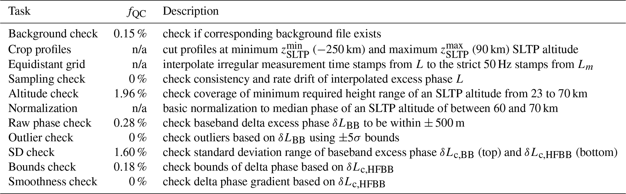
The QC process starts from raw excess-phase data (raw signal) with some basic data preparation steps and initial checks for physical plausibility of the measurement. Initially, all the profiles are cropped to a minimum of km and a maximum of km altitude, respectively. Subsequently, the measurements, recorded at irregular measurement times, are interpolated to a strict equidistant time grid of 50 Hz based on the model grid. Additionally, the sampling rate consistency and drift are checked to be within the plausible maximum limits of 0.015 s and 10−5 s min−1, respectively, over the entire cropped altitude range. The interpolated and cropped excess-phase profiles are written to the output used for further L1b processing; all subsequent steps solely serve the quality control and are stored as interim output.
For further processing, profiles which do not span over a minimum altitude range from km to km are dismissed or optionally flagged. In a next step the entire profile is normalized to the median value of an SLTP altitude between 60 and 70 km. In order to eliminate obviously unphysical profile behaviors, delta profile δLBB for any signal profile is not allowed to exceed 500 m (an empirically determined value for sorting out gross outliers) over the minimum SLTP altitude range defined above.
Highly important to the QC, as well as for safeguarding the further processing, is the outlier detection performed on baseband delta excess phase δLBB for each signal profile separately. This baseband delta excess phase allows for a very robust outlier check, since the forward-modeled excess phase is a noise-free reference, in order to focus on potential irregular spikes and patterns in the data themselves. The outlier detection criteria are based on a moving-median-referenced percentile-based detection calculation. The 16th and 84th percentile are used for an estimation of the standard deviation (±σ). A data point is considered an outlier if it is greater than the 5-fold value of this standard deviation around the median; if more than 3 % of outlier values are detected across the profile, the entire profile gets rejected.
Since values are not distributed symmetrically around the median, an adequate window size of data points was found as a result of sensitivity tests that evaluated statistics and counted the number of profiles with at least one detected outlier, while employing different window sizes (Seidl, 2018). At this stage of the processing, outliers are only detected, while in the early part of the ODP L1b processing outliers are then (statistically) corrected, because further calculations including averages and standard deviations respond very sensitively to outliers. That correction replaces any detected outlier value by a statistically reasonable value randomly drawn from a normal distribution with standard deviation within the interval [−3σ, +3σ].
Next, inspection of the moving standard deviation of delta excess-phase profiles, using a window size of data points to estimate it, helps to estimate reliable top and bottom altitude levels, within which the quality of the excess-phase data is considered sufficiently reliable to retrieve sufficiently accurate variables in the subsequent geometric-optics bending-angle retrieval. For the determination of a reliable top altitude level in the mesosphere, we apply a moving standard deviation to baseband delta excess phase δLc,BB and check where a threshold of 3 cm (an empirically determined reasonable value) is exceeded for the first time when searching upwards.
For determination of the bottom altitude level, the standard deviation of high-pass-filtered baseband delta excess phase δLHFBB of L1, L2, and Lc profiles are checked, now searching downwards, for the maximum of either a fixed value (3 cm) or a relative value (0.1 %), the latter relative to forward-modeled excess phase Lm. If the moving standard deviation thresholds are found to be exceeded already within the minimum-required altitude region from to , then the respected profile (and whole RO event) is either discarded or flagged. The top and bottom altitude levels determined are stored for later use, such as for optionally cutting the profiles to their best-quality range before further retrieval steps.
A final pair of fundamental QC checks for the physical plausibility of a processed excess-phase profile is done by checking the bounds and smoothness of delta excess-phase profiles of Lc. The bounds are checked on baseband delta excess phase δLc,BB with defined limits derived from sensitivity studies and using general physical knowledge for expected magnitudes in different atmospheric altitude regions. Specifically, every data point of δLc,BB is checked to be within a threshold of 15 cm in the mesosphere from 50 km upwards and the maximum for altitudes from 30 km downwards, respectively. For altitudes in between (upper stratosphere), the bound is defined by linearly increasing between the lower-stratospheric and mesospheric bounds, i.e., from 30 to 15 cm (Seidl, 2018).
The smoothness check is based on a five-point derivative of high-pass-filtered baseband delta excess phase δLc,HFBB, yielding a delta phase derivative profile used for detection of rapidly fluctuating noise or spikes with unphysical magnitude. The smoothness bound is set such that no point in the derivative profile shall exceed 7.5 m s−1. Additionally, it is cross-checked to fall within a relative limit of 75 % of the five-point derivative of Lm. Profiles failing the bounds check and/or smoothness check within the minimum-required altitude range are discarded.
3.2.2 Characterization of excess-phase uncertainty
Following the QC of the RO events initially processed by the ODP L1a processor (raw), the uncertainty in the excess-phase profiles found to be of adequate quality (i.e., passing the QC) is characterized and empirically estimated as the next step of the processing. This new approach to assess the uncertainty in each individual RO event is conducted following the Guide to the Expression of Uncertainty in Measurement (GUM; JCGM2008, JCGM2012) and its proposed handling and terminology of uncertainties. Overall the GUM is considered the standard guideline for the uncertainty estimation and propagation in rOPS, as already realized in parts of the retrieval (Innerkofler et al., 2020; Schwarz et al., 2017, 2018; Schwarz, 2018; Li et al., 2019).
As summarized by Schwarz et al. (2018) we categorize uncertainties into estimated random uncertainties and estimated systematic uncertainties, the latter with differentiation between basic and apparent systematic uncertainties. Effects included in the estimated random-uncertainty budget are of unpredictable or stochastic temporal and spatial variability in repeated observations. These effects are essentially stationary in a statistical sense so that we can estimate their statistics also from individual RO event data, given the high noise-resolving sampling rate along the vertical profile.
Systematic effects (biases), which can not be quantified using statistical data analysis based on just one individual RO profile, are estimated and corrected for if known, as recommended by the GUM. The remaining residual biases are assumed to stay within a (conservative) bound estimate, which we refer to as estimated systematic uncertainty. Depending on their nature, we distinguish two types: (1) estimated basic systematic uncertainties which appear and will remain systematic despite averaging over individual RO events and (2) estimated apparent systematic uncertainties which will essentially behave as random uncertainties in ensemble averaging over many RO events. It is important to distinguish these two subtypes, since the former will not average out and therefore fundamentally limit the (absolute) accuracy of ensemble averages such as climatologies.
With respect to the phase observations (Eq. 4) a total uncertainty budget for the GNSS excess-phase measurements can be approached as
where utot denotes the total uncertainty assigned to the excess-phase profile, uatm denotes the uncertainty inferred from the neutral atmosphere influences, uion denotes the uncertainty inferred from the ionospheric influences, ur,clk denotes the receiver clock uncertainty, ut,clk denotes the transmitter clock uncertainty, uvel denotes the velocity drift uncertainty, utherm denotes the thermal noise, umult denotes uncertainty due to local spacecraft multipath, ucycle denotes the cycle slip uncertainty, and uphase denotes the phase noise comprising residual error influences.
Remaining error sources, such as phase wind-up and tide and ocean loading effects, which are not considered in Eq. (11), are expected to be below the order of 10−6 in relative errors and are therefore disregarded in the uncertainty budget. Not yet taken into account is the spacecraft's attitude uncertainty which will be addressed in more detail once the attitude correction in rOPS is included and verified. For larger spacecrafts like the Metop satellites this effect caused by attitude jitter is expected to be small, however. Also interpolation and the smoothing of data introduce errors in the calculations, e.g., by disregarding terms of a higher order in an approximation or through the imperfect representation of numerical values. Within the excess-phase processing these errors are mostly attributable to the interpolation of the receiver and transmitter orbits and clocks. The magnitude of these errors was empirically determined and found to be smaller than the order of 10−5 in relative errors and hence is also considered negligible compared to the other components in the error budget.
The uncertainties in the transmitter and receiver clocks are modeled based on their 1 s Allan deviation, using typical values for atomic clocks and quartz clocks of GNSS and LEO satellites, respectively (cf. Sect. 3.1.3). The relative frequency error for white frequency noise averaged over the sampling time is simply simulated as a random number between −1 and 1 (Harting, 1996). To achieve the correct 1 s Allan deviation of the final calculated clock noise, the 1 s Allan deviation has to be corrected for the used sampling rate. The relative frequency error for the sampling period therefore becomes
where yn is the relative frequency error averaged over the sampling period τs, A1sec is the 1 s Allan deviation, randn is the random number between −1 and 1, and c is the speed of light in a vacuum. For spaceborne single differencing, a flicker frequency noise is added to the clock uncertainty.
Thermal noise denotes the errors due to the random movements of electrons in the electronic components of a GNSS receiver. For carrier phase signals of nominal strength, the thermal noise in the carrier-tracking phase-locked loop (PLL) of a GNSS receiver can be modeled as
where BL is the carrier loop noise bandwidth, is the carrier-to-noise power density ratio, and λ is the carrier phase wavelength. In a realistic approximation, with dB Hz and BL=2 Hz, the thermal noise for the GPS L1 signal is 0.2 mm (Langley, 1997). Accounting for the weaker GNSS signals and non-optimal conditions in the lower atmosphere, where open-loop tracking is also used, we safely assume a conservative bound for the influence of the thermal noise on phase measurements of 1 mm for all measured GNSS signals.
The random velocity error, estimated along with the POD processing (Sect. 2.2.1), also contributes to the total uncertainty budget. It introduces a linear drift to the measurement and is therefore categorized as estimated apparent systematic uncertainty. Assuming a random velocity uncertainty in mm s−1 of the receiver satellite orbit,
where the total uncertainty introduced by the velocity drift uncertainty uvel would account for 1.2 mm after a typical RO event duration of 60 s from the time of the highest altitude ttop to the lowest altitude tbot.
As stated in Sect. 3.1.1, phase ambiguities do not pose a problem in the excess-phase processing since constant terms can be eliminated from the observation equation. However, an undetected cycle slip can introduce a phase shift of half or full carrier wave cycles on the order of several centimeters, depending on the wavelength of the GNSS frequency. With decreasing altitude the ratio between the absolute value of the excess phase and the magnitude of possible cycle slips increases, and additionally propagation media effects in the troposphere require a DLL measurement mode, which makes cycle slips occur more frequently and leaves them undetected. Therefore, to account for these undetected cycle slips as an estimated basic uncertainty, we include change-rate factor c=1 mm s−1, reflecting a 1 % slip fraction per second relative to the half-cycle length. This leads to a gradual excess-phase decrease (cumulative negative bias) with decreasing altitude from the time of highest altitude to lowest altitude in the DLL measurement mode:
A local spacecraft multipath occurs when the incoming signals at the receiver satellite are reflected and scattered before reaching the vicinity of the GNSS antenna, and thus signals with different paths are detected simultaneously at the receiver. The effect depends on the spacecraft geometry, the occultation viewing geometry, and the electrical properties in the vicinity of the receiver antenna (Kursinski et al., 1997). The possible phase shifts of up to a few centimeters, introduced by the local spacecraft multipath, can be reduced by proper platform design and the use of directional antennas. Additionally, local multipath effects can be reduced by dismissing incoming left-hand polarized signals, since the right-hand circular-polarized GNSS signals are left-hand polarized after reflection at the surface of the LEO. The residual local multipath error effects on the phase measurements are modeled using a sinusoidal model, for representative broad beam antennas used in GNSS RO (Steiner and Kirchengast, 2005; Ramsauer and Kirchengast, 2001; Syndergaard, 1999). The sinusoidally shaped function is defined with a multipath phase error amplitude of 0.5 mm and period set to 60 s, resulting in multipath errors up to 1 mm, following GRAS-type error specifications (Carrascosa-Sanz et al., 2003). We classify this effect as apparent systematic uncertainty, since with a changing viewing geometry from occultation to occultation, the local spacecraft multipath errors will average down when regional and temporal averages are calculated (Kursinski et al., 1997).
The influence of the propagation media (neutral atmosphere and ionosphere) itself cannot be quantified directly because ionospheric scintillations and atmospheric turbulence lead to variations in the properties of the atmosphere which can be hardly captured by models. However, if we assume that the defined uncertainty budget in Eq. (11) includes all possible major error sources, the uncertainty arising from the neutral atmosphere and ionosphere can be inferred from an empirical estimate of the total random uncertainty and subtraction of the terms categorized as contributors to the random uncertainty:
The empirical uncertainty estimate is determined based on the double-delta excess-phase profiles δLHFBB smoothed with a moving standard deviation with a window size of , like we already used in in the QC processing (Sect. 3.2.1).
As the final output, the combined estimated random, basic systematic, and apparent systematic uncertainties are appended to the L1a output, while the individual uncertainty estimates are stored in a “monitoring file” together with the QC output. Figure 8 illustrates the daily component-wise and combined uncertainty estimates. The overall estimated excess-phase uncertainties then serve as input to the subsequent uncertainty propagation in the ODP L1b bending-angle retrieval (Schwarz et al., 2018). An evaluation of the uncertainty estimation can be found in the results in Sect. 4.3.
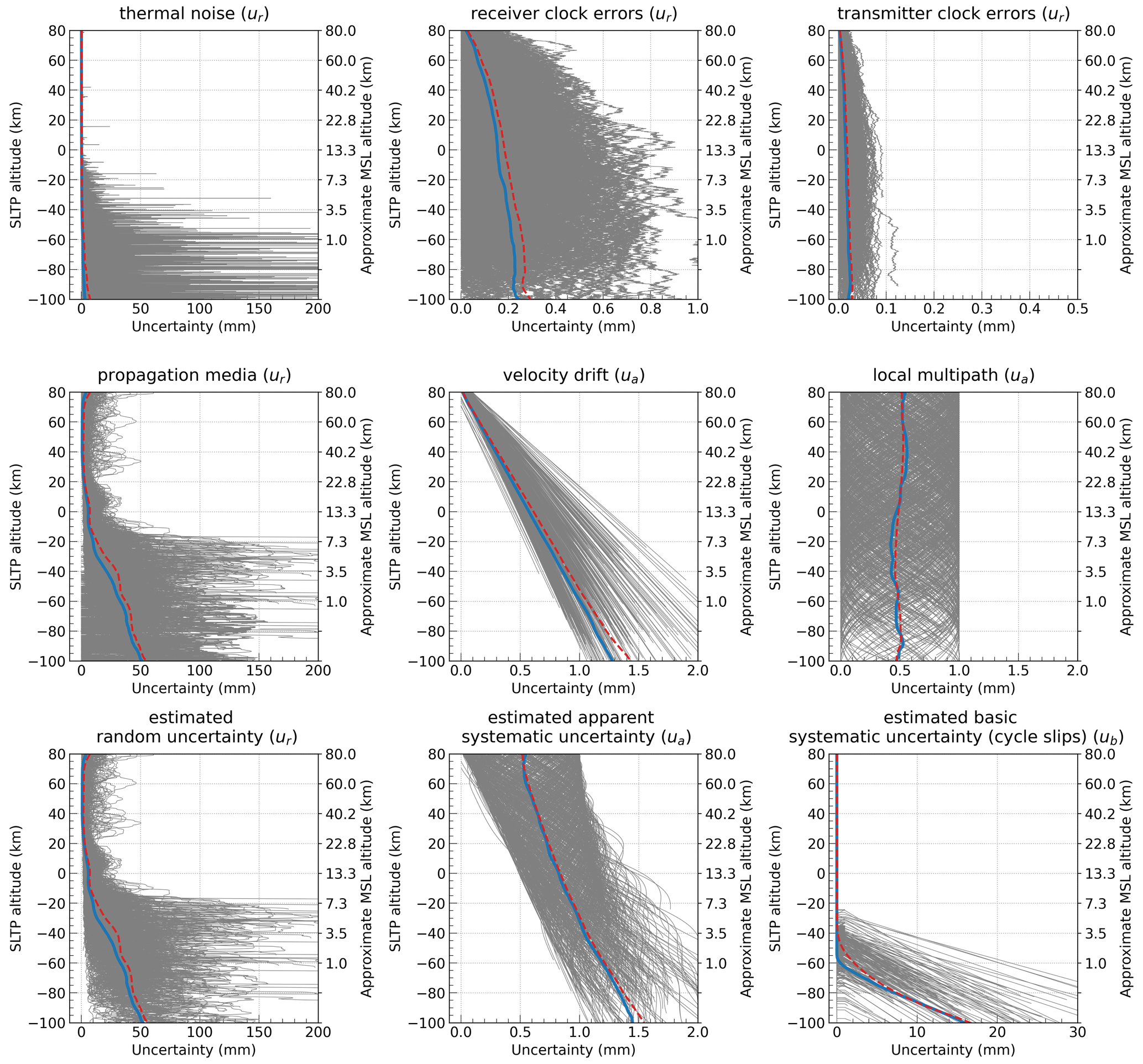
Figure 8Overview of exemplary estimated random ur, basic systematic ub, and apparent systematic ua uncertainty components, respectively, from rOPS ODP L1a processing for Metop-A on 1 July 2008. For each component, individual estimates for each of the 781 events (thin grey profiles) are shown together with the daily median (highlighted thick blue) and mean (highlighted dashed red) uncertainty profile.
In this section we evaluate a set of three 3-monthly periods of RO data at the excess-phase level, the summers of 2008 and 2013 (both July–August–September, JAS) and the winter of 2019/20 (December–January–February, DJF), for the Metop-A/B/C RO data as available given their launch times. Starting with a sensitivity analysis of the excess phases computed by rOPS, we analyzed how the measured profiles compare against forward-modeled profiles, how a different orbit solution input influences the L1a excess-phase processing, and how the evaluated differences in collocated profiles agree between the three Metop missions and their GRAS receivers.
Subsequently, we present a statistical ensemble evaluation of WEGC's rOPS data in comparison to the excess-phase data processed and provided by EUMETSAT and UCAR. The last subsection discusses results related to uncertainty estimation of the excess-phase profiles processed at WEGC.
The number of profiles for each study period per Metop satellite is depicted in Fig. 9. All data are available in the rOPS-L1a file format, where the external excess-phase data from EUMETSAT and UCAR underwent a basic conversion routine. Overall, on average, the daily number of profiles amounts to 647 profiles (Metop-A), 610 profiles (Metop-B), and 559 profiles (Metop-C). For the later 2020 JAS period EUMETSAT input data contain files with a missing closed loop (either L2 or both frequencies), which reduces the number of processed events in this later study period, with reduced numbers in the later periods. In the following evaluation, differences between observations of rising or setting RO events or differences from geographic regions (zonal bands) are discussed whenever worthwhile to take into account.
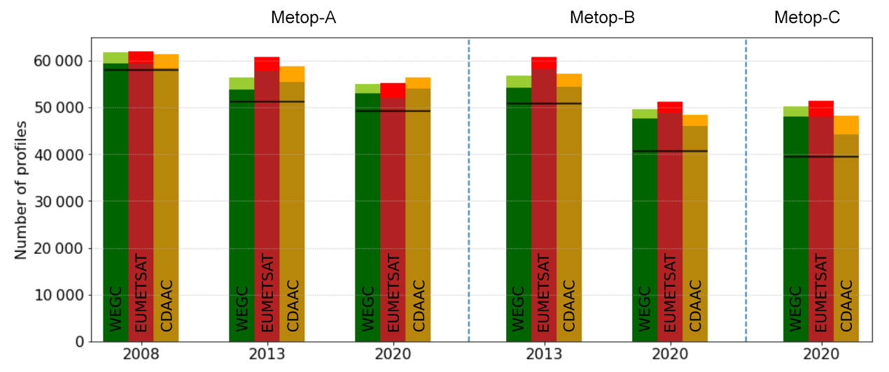
Figure 9Number of RO events per time period (2008-JAS, 2013-JAS, 2020-DJF) processed at WEGC (green) and converted from EUMETSAT (red) and CDAAC (orange) to the rOPS format. Darker shaded area of the bars indicates profiles which successfully passed quality control. The black line indicates the number of profiles matched by the event identifier and common to all three processing centers.
4.1 Sensitivity analysis
In order to evaluate the quality of processed excess phases and their sensitivity to certain effects we considered their difference to selected reanalysis data, their sensitivity to different orbit inputs and different measurement geometries, and their dependency on the specific Metop satellite. For a comprehensive and very comparative analysis we focused on three vertical atmospheric regions and their layer averages (calculated from the vertical statistical measures, i.e., mean, median, SD, and percentiles, by obtaining the average over all values within the corresponding altitude layer):
-
Middle troposphere (3–7 km). This atmospheric region in the lowermost section of the atmosphere was selected for representation of the (moist) middle to lower troposphere. With the restriction of being above 3 km, the boundary layer and its special behavior that requires separate study (e.g., Gorbunov et al., 2021; Gorbunov and Kirchengast, 2018; Zeng et al., 2016) were disregarded.
-
Lower stratosphere (20–25 km). This region represents the lower-stratosphere region of RO soundings, with narrow uncertainty and minimal influence of background data or of any tropospheric or tropopause effects in the retrieval.
-
Lower mesosphere (50–60 km). This region represents the lower mesosphere with small absolute excess phases only on the order of 10 cm left but still without major ionospheric influences that start higher. The layer thickness of this region is increased compared to the tropospheric and stratospheric layers for increasing averaging in view of the less dense atmosphere at these higher altitudes.
4.1.1 Atmospheric-background modeled profiles: O−B
The observed RO data, processed to the excess-phase level by WEGC's rOPS, are compared to forward-modeled excess-phase background profiles from ECMWF ERA5 reanalyses (Sect. 2.2.3) in an observation minus background (O−B) comparison. Since per construction there is a corresponding reference profile extracted from the highly resolved ECMWF data for each observed RO event, the number of profile pairs is high.
Statistical evaluation of WEGC processing against the forward-modeled atmospheric-background profiles is shown in Fig. 10. In general the median of the intercomparison is seen at the millimeter level for all atmospheric regions and Metop satellites considered. The spread of the data increases due to higher variability and model imperfections at lower altitudes in the troposphere, where also a portion of skewed data can be seen. Differences between rising and setting RO events and differences in geographic distribution (not shown) are found to be very small with median differences of a few millimeters.
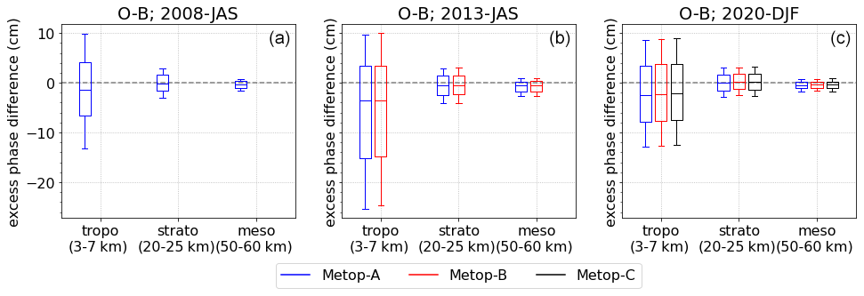
Figure 10Sensitivity analysis results from comparing WEGC rOPS L1a excess-phase profiles from Metop-A (blue), Metop-B (red), and Metop-C (black) against collocated forward-modeled profiles from ERA5, for the three 3-month periods (2008, 2013, 2020; a to c) and three representative altitude layers (a to c within each panel), with the box and whiskers depicting the median (mid-line), 16 %–84 % range (box), and 5 %–95 % range (whiskers).
4.1.2 Orbit sensitivity
Various studies have documented that the accuracy of the orbit and, in particular, the velocities and estimated clock biases, co-determine the quality of the derived excess-phase profiles (e.g., Kursinski et al., 1997; Montenbruck et al., 2008). For this reason, WEGC implemented a novel system routinely evaluating the quality of the calculated orbits which was introduced by Innerkofler et al. (2020). In this study we conducted the WEGC L1a excess-phase processing based on three different orbit solutions, from WEGC, EUMETSAT, and UCAR, respectively.
The comparison results of these independently computed orbit solutions are summarized in Table 5. These results focus on 2013-JAS and 2020-DJF, since data from 2008 were not available from EUMETSAT for this study part. In order to ensure a stable orbit geometry and excess-phase comparison, one generally aims for a daily 3D rms (root mean square) threshold of 5 cm in position and 0.05 mm s−1 in velocity (Innerkofler et al., 2020). This is generally satisfied for the WEGC orbit solutions in comparison to EUMETSAT, whereas UCAR exhibits slightly higher deviations as part of this intercomparison.
Table 5Metop orbit intercomparisons for position and velocity in terms of 3D rms for different orbit solutions for the 2013-JAS and 2020-DJF periods, compared to the EUMETSAT–NAPEOS POD solution used as a reference. Days flagged to exceed 20 cm in 3D rms (about 3 d per satellite and 3-month period) have been excluded from the statistics.
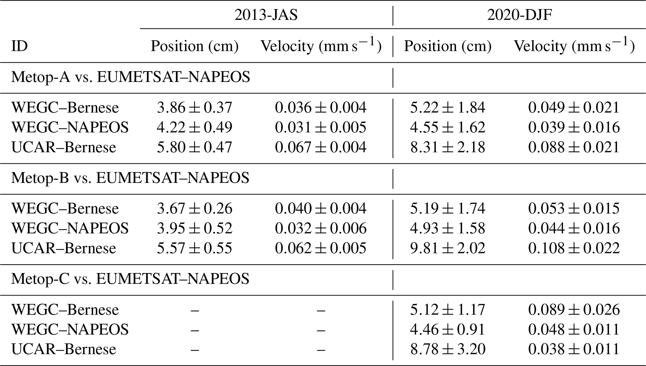
Comparison results of rOPS-processed excess phases based on WEGC–Bernese and orbit processing against using EUMETSAT POD exhibit a similar agreement across all vertical layers, time periods, and satellites. As depicted in Fig. 11, the median of the comparison experiences a slight positive bias and is enclosed by a stable percentile envelope, which is only slowly increasing when moving towards lower-atmospheric regions. Overall, the 5th–95th percentile range stays below about 1 cm. Setting events show a tendency, at the millimeter level, towards smaller averages and rising events towards larger averages, compared to the total median statistic.
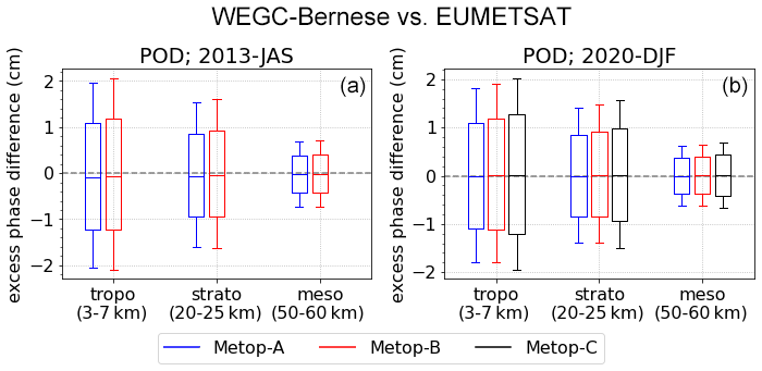
Figure 11Sensitivity analysis results from comparing WEGC rOPS L1a excess-phase profiles from Metop-A (blue), Metop-B (red), and Metop-C (black) based on WEGC–Bernese orbits minus excess-phase profiles based on EUMETSAT POD solutions, for the two 3-month periods (2013, 2020; a to b) and three representative altitude layers (a to b within each panel), with the box and whiskers depicting the median (mid-line), 16 %–84 % range (box), and 5 %–95 % range (whiskers).
4.1.3 Sensitivity of sensors
In order to investigate the influence and difference between the very similar receivers and satellite platforms, profiles of the three Metop satellites were co-located and binned together, before these differences were also calculated for statistical inspection. Though the satellites are essentially identical in construction, different firmware, a shift in orbital planes, different satellite lifetimes, and the degradation of instruments and hardware may influence the differences between profiles of different satellites.
For the evaluation of platform-dependent differences the collocation algorithm was restricted to match profiles within 2 h in time and 200 km in space. In addition to this, we limited the analysis to the period where at least the first two satellites launched, Metop-A and Metop-B, were already in space. This results in an adequate number of co-located profiles for robust statistics: 2708 (2013-JAS) and 1641 (2020-DJF) for Metop-B vs. Metop-A and 1797 (2020-DJF) for Metop-C vs. Metop-A.
Figure 12 shows that the resulting differences are generally larger compared to strictly collocated profile-to-profile comparisons, particularly in the troposphere, where the space–time mislocation of the RO event locations grossly dominate the (quasi-random) differences. However, the results exhibit a stable median, which is well centered at 0 (centimeter-level consistency) for all altitude layers. Only for Metop-C in winter 2020 is a small positive deviation from 0 visible for the tropospheric layer, which is due to the high overall variability that cannot be interpreted in more detail based on these statistics.
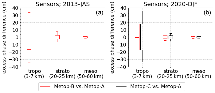
Figure 12Sensitivity analysis results from comparing co-located WEGC rOPS L1a excess-phase profiles from Metop-B (red) and Metop-C (black) against Metop-A, selected as a representative reference, for two 3-month periods (2013, 2020: a to b) and three representative altitude layers (a to b within each panel), with the box and whiskers depicting the median (mid-line), 16 %–84 % range (box) and 5 %–95 % range (whiskers).
4.2 Statistical analysis
In order to evaluate the performance and ensure the highest-quality profiles by the new rOPS L1a processing, the excess-phase profiles calculated at WEGC were also evaluated against profiles from EUMETSAT (von Engeln et al., 2009) and UCAR CDAAC (Schreiner et al., 2011), the latter serving as an additional independent data source. Prior to comparison and the calculation of profile differences, the external L1a profiles from EUMETSAT and UCAR were converted to the rOPS-L1a format, including the calculation of a consistent and unambiguous event information identifier and some format alignments of the datasets (Sect. 2.2). This enables reliably matching the RO events from the three different processing centers.
For a thorough analysis we separated the profiles into a combined mesospheric and stratospheric section, using MSL altitude (mapped using the corresponding forward-modeled profiles) as a vertical coordinate from 10 to 80 km. In this range, absolute phase and differences are comparatively small. Second, a tropospheric region using SLTP altitudes from 0 to −100 km was defined, wherein loss of lock of the tracking usually occurs and where open-loop tracking introduces larger differences. Considering a standard-atmosphere model, this approximately equals an MSL altitude from about 13 km down to the last few hundred meters above Earth's surface within the boundary layer.
Although several profiles reach down to an SLTP altitude of −250 km, the number of profiles significantly decreases below an SLTP altitude of about −100 km, which is why we focused the tropospheric statistics down to this level. Furthermore, strong refraction, possibly super-refraction, and other disturbances complicate an overall statistical comparison at the very low-altitude levels below an SLTP altitude of −100 km.
Figure 13 shows the number of available matched profiles from WEGC and CDAAC vs. EUMETSAT for 2008-JAS, 2013-JAS, and 2020-DJF, for all RO events from Metop-A/B/C and additionally separated for rising and setting events. In comparison, generally the number of profile differences from setting events, compared to rising events, is higher for all time periods and also shows an overall deeper penetration.
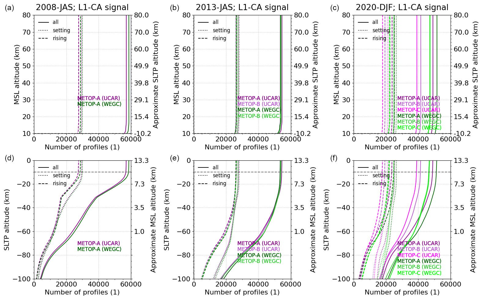
Figure 13Number of excess-phase difference-pair profiles used for the ensemble statistics for WEGC vs. EUMETSAT (green) and WEGC vs. UCAR (purple), with a focus on (a–c) the stratosphere and mesosphere region and (d–f) the troposphere region. Difference-pair profile numbers are shown for L1–CA excess-phase profiles, featuring the deepest penetration and being most relevant for the subsequent L1b retrieval.
The inter-center comparison results at the excess-phase level between WEGC and UCAR against EUMETSAT (the latter used as a reference) are shown in Fig. 14 for the stratosphere-/mesosphere-focused region and in Fig. 15 for the troposphere-focused region, respectively.
A closer look at these 3-monthly excess-phase difference statistics as a function of MSL altitude (see Fig. 14) shows good agreement and robust difference statistics. The systematic difference between WEGC and EUMETSAT shows a virtually bias-free consistency (differences within 1 mm), apart from the 2013 period, where a salient kink can be observed at an MSL altitude of around 11 km. More detailed investigation showed that this behavior occurs for all time periods considered, although the altitude at which it can be observed is slightly below an MSL altitude of 10 km for the other time periods and hence outside the focus region shown in Fig. 14.
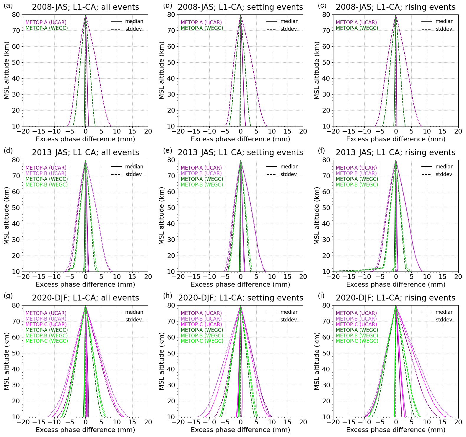
Figure 14Systematic difference (median) and standard deviation (16th and 84th percentile) profiles from the statistical ensemble differences between excess-phase profiles from WEGC (green) and UCAR/CDAAC (magenta) compared to EUMETSAT. (a, d, g) All events, (b, e, h) setting events, and (c, f, i) rising events are shown for (a–c) 2008-JAS to (g–i) 2020-DJF. The altitude range focuses on an MSL altitude of 10–80 km.
This characteristic can be attributed to a weakness in the transition from closed-loop to open-loop data for rising events in the WEGC processing, a matter which is currently under refinement. Systematic differences between UCAR and EUMETSAT show a positive bias, up to 2 to 3 mm, around the tropopause, which is most pronounced for setting events. Interestingly, in 2020-DJF the biases for rising events prevail. With increasing excess-phase magnitude, with decreasing height, the standard deviation of the comparison of WEGC with EUMETSAT also gradually increases, from 80 km down to 10 km in a linear and fairly symmetrical manner. The standard deviation of the differences corresponds to an envelope of about ± 6 and ± 8 mm (somewhat increased in 2020), demonstrating millimeter-level consistency of the random deviations. With UCAR as the candidate dataset, slightly increased standard deviations on the order of 1 cm can be observed near an altitude of 10 km.
The statistical intercomparison in the troposphere, depicted in Fig. 15, shows a good agreement between WEGC and EUMETSAT excess-phase profiles, with an almost bias-free comparison down to about an SLTP altitude of −80 km and a slightly increased systematic difference below. Separate investigation of rising and setting events reveals increased systematic differences starting already at about −50 km for rising events. However, the contribution to the overall statistics is limited because of the lower number of rising profile differences in that altitude region (cf. Fig. 13).
For the intercomparison statistics of UCAR against EUMETSAT, increased systematic differences are found starting at about −40 km in 2013-JAS and 2020-DJF, a characteristic only found below about −80 km in 2008. The biases observed are similar for all Metop satellites and most pronounced for setting events in 2020-DJF. At about −100 km, their magnitude is on the order of about 4 times the signal's wavelength, while rising events feature smaller but positive biases.
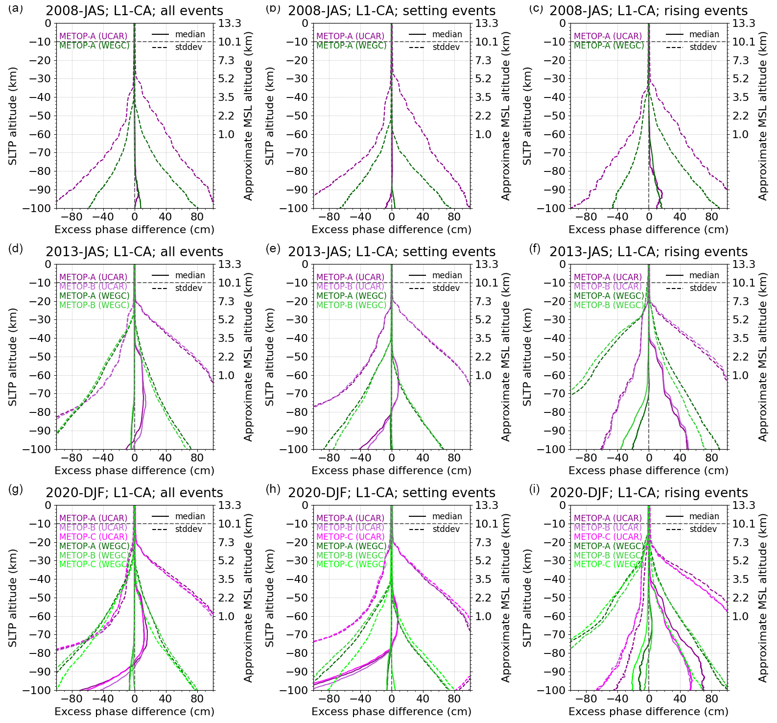
Figure 15Systematic differences (median) and standard deviation (16th and 84th percentile) profiles from the statistical ensemble differences between excess-phase profiles from WEGC (green) and UCAR/CDAAC (magenta) compared to EUMETSAT. (a, d, g) All events, (b, e, h) setting events, and (c, f, i) rising events are shown for (a–c) 2008-JAS to (g–i) 2020-DJF. The altitude range focuses on an SLTP altitude of −100–0 km.
Although these characteristics arise in the (deep) boundary layer, where proper signal tracking is challenging, the salient deviations between UCAR excess phases and EUMETSAT and WEGC processing results point to remaining issues in the different processing approaches. However, such further investigation is beyond the scope of this study and will be addressed in follow-on intercomparison work.
The standard deviation of the comparison statistics shows an increase in the spread of the data with the onset at an SLTP altitude of about −20 km for the comparisons from WEGC and UCAR against EUMETSAT, along with a decreasing number of difference-pair profiles. For setting events considered separately, however, the standard deviation for WEGC against EUMETSAT is narrower and starts to increase from an SLTP altitude of −50 km downwards. In general, the standard deviation amounts to about ± 80 cm in most cases at an SLTP altitude of −100 km, with increased values for UCAR compared to WEGC as a candidate dataset in the lowest hundreds of meters of the boundary layer close to Earth's surface.
4.3 Uncertainty analysis
As described in Sect. 3.2.2, the empirical uncertainty estimation at the excess-phase level delivers estimated random uncertainty and, separately, estimated basic and apparent systematic uncertainties for each individual RO event. Related to this Fig. 16 provides, as a synthesis result, a concise overview of daily mean estimates of these uncertainties, for a representative example day of each of the three 3-month periods investigated.
In the mesosphere and upper stratosphere, the estimated random- and systematic-uncertainty components are small at the millimeter level, while towards lower altitudes, where the absolute excess phase increases rapidly, the estimated random-uncertainty component amounts to several centimeters (which is still very small at levels below 0.02 % in relative terms in the troposphere, though). The estimated systematic-uncertainty component is seen to be very small at the millimeter level and increases with decreasing altitude to reach about 2 cm in the deep troposphere.
Overall, the daily averages of the uncertainty estimates as depicted in Fig. 16 show similar characteristics for all three time periods and for all the three different Metop satellites. However, between an SLTP altitude of −20 and −40 km, the two later periods exhibit a slight kink in the estimated random uncertainty compared to the 2008 period. This is presumably connected to the different structure of the corresponding numbers of profiles as a function of altitude shown in the lower panel of Fig. 13 and changes in the receiver tracking.
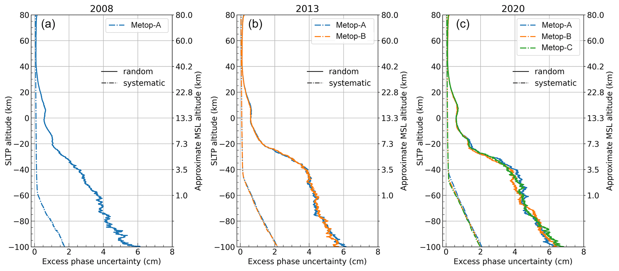
Figure 16Daily averages (median) of estimated random and estimated systematic (combined basic and apparent) uncertainties based on uncertainty profiles of an individual RO event for the example days of 1 July 2008 (Metop-A; a), 1 July 2013 (Metop-A/B; b), and 2 January 2020 (Metop-A/B/C; c).
The derivation of climate benchmark data from RO measurements requires a rigorous processing from the raw GNSS signal occultation measurements (including their georeferencing in space–time) to essential climate variables (ECVs), such as temperature, with narrow uncertainties. In order to encompass the entire RO data processing, the new rOPS processing system at WEGC has recently seen major advancements in Level 1a (L1a) processing, with the integration of the POD processing (Innerkofler et al., 2020) as well as the excess-phase processing including uncertainty estimation that was presented and evaluated in this study.
The rOPS L1a excess-phase processing, itself algorithmically concise, is complemented by integrated quality control and uncertainty estimation, which requires an advanced framework of various subsystems, which we introduced in a step-by-step manner in Sect. 2. Starting with the input data preparation we discussed the various input data sources. Building on the POD processing, integrated in rOPS, the DSM (daily system modeling) subsystem delivers daily LEO receiver and GNSS transmitter satellite orbit and clock data. The observation geometry setup computed by ESM (event system modeling) facilitates the provision of basic event-based geometry and environmental context information. Complemented by atmospheric profiles modeling, ESM also provides reliable forward-modeled excess-phase profiles based on collocated (re)analysis data such as from the ECMWF Reanalysis (ERA5). These forward-modeled profiles, including a forward mapping of mean sea level (MSL) altitudes to the RO event's time grid, are found to be highly valuable for the quality control and for supporting the uncertainty estimation.
After the introduction of the rOPS L1a processing framework, we provided an in-depth description of the main processing algorithms for the derivation of excess-phase profiles in addition to a due account of the GNSS observables and corresponding receiver-tracking modes. Subsequently, an elaborated quality control, to a major extent supported by forward-modeled excess-phase profiles, removes or alternatively flags profiles of insufficient or degraded quality. The primary addition, however, is the component-wise estimation of excess-phase uncertainty profiles for each individual RO event, which serve as a starting point for the uncertainty propagation in the subsequent RO retrieval chain down to the atmospheric ECV profiles.
The validation of the new processing was based on three 3-month periods (in 2008, 2013, and 2020) for achieving a robust statistical analysis. In a sensitivity analysis for inspecting the quality and reliability of the resulting excess phases, we focused on three atmospheric layers – lower mesosphere (50–60 km), lower stratosphere (20–25 km), and middle troposphere (3–7 km) – investigating differences between observed and collocated ERA5-derived profiles, the influence of different orbit and clock inputs, and a cross-platform comparison between profiles from the different Metop satellites.
The comparison against forward-modeled profiles revealed small systematic differences mostly of the millimeter level only, based on the multi-monthly statistics. The exchange of WEGC LEO orbit solutions with orbit solutions from EUMETSAT or UCAR (all of adequate quality within about 5 cm in position and 0.05 mm s−1 in velocity in an orbit intercomparison) in the rOPS processing led to negligible differences in the results of the different time periods and Metop satellites. Intercomparing matched observations between different Metop satellites, using collocation criteria of 2 h in time and 200 km in space, revealed larger differences dominated by the space–time differences in the RO event locations, but still the median difference results, found at millimeter-level deviation, confirmed an overall statistically very tight consistency across the different Metop receiver platforms.
An inter-center comparison of WEGC- and UCAR-processed excess phases against EUMETSAT-processed data focused on an upper- (MSL altitudes of 10–80 km) and lower-atmospheric (SLTP altitude from 0 to −100 km) region, respectively. While this analysis revealed some small discrepancies in the processing of rising RO events at WEGC, the excess phases processed with rOPS show better agreement to EUMETSAT excess phases than to UCAR ones. In the stratosphere-/mesosphere-focused region, the differences between WEGC and EUMETSAT amount to 1 ± 6 mm, compared to 3 ± 8 mm for UCAR against EUMETSAT. In the troposphere-focused region, differences stay small down to an SLTP altitude of about −80 km, with a standard deviation increase to near ± 80 cm, still corresponding to very small relative differences. Larger deviations of UCAR excess phases at lower altitudes suggest noticeable differences compared to the processing strategies at WEGC and EUMETSAT.
A sensitivity check of the stability of the uncertainty processing, based on daily averages of example days from the study time periods, showed closely consistent systematic- and random-uncertainty estimates across all time periods and the three Metop satellites. Both the estimated random and estimated systematic uncertainties stay at the (sub)millimeter level in the stratosphere and mesosphere, while at tropospheric altitudes in the dense atmosphere with large excess phases, where signal tracking is challenged, the random-uncertainty estimates increase up to several centimeters.
We note that the results from the intercomparison between excess-phase data processed by EUMETSAT, WEGC, and UCAR experience larger differences in the lower troposphere than we quantified in the uncertainty budget. This indicates additional structural uncertainties arising from different processing schemes not captured in the estimated uncertainties in the observational data. In order to address this substantial differences, a broader inter-center comparison study is advised.
In follow-on work we will investigate the long-time evolution of the uncertainty budget and compare the characteristics to those of other RO missions. The approach of the uncertainty estimations of various components at the excess-phase level is also subject to repeated improvements and refinements. Overall the results provide evidence for the rOPS L1a processing's capability to provide valuable uncertainty estimates for further processing, supported by rigorous quality control for climate quality data-processing demands. Demonstrating the delivery of robust and accurate excess-phase profiles, the results indicate that the rOPS L1a subsystem is a reliable new excess-phase processor, which is versatile also in the sense that it can handle multiple different input data sources, such as orbit and excess-phase data also from other processing centers.
While this study focused on a thorough introduction and careful initial evaluation based on Metop-A/B/C satellite data, the rOPS L1a processing is set up as a multi-mission system capable of processing RO measurements also from the CHAMP, GRACE, COSMIC, COSMIC-2, FY-3, and Spire RO satellite series. In this way it will support the provision of long-term multi-mission RO data records including uncertainty estimation, for the benefit of climate monitoring and research.
The code used to produce the results of this study is available from the corresponding author upon qualified request.
The (numeric) data underlying the results of this study are available from the corresponding author upon qualified request. Excess phase data from EUMETSAT supporting this study are available at https://doi.org/10.15770/EUM_SEC_CLM_0029 (EUMETSAT, 2020). Supporting data from UCAR-CDAAC were downloaded from https://doi.org/10.5065/789w-m137 (CDAAC, 2023a), https://doi.org/10.5065/1k0w-2272 (CDAAC, 2023b), and https://doi.org/10.5065/p8es-mc74 (CDAAC, 2023c). Atmospheric field data from ERA5 global reanalysis are available at https://doi.org/10.24381/cds.143582cf (Hersbach et al., 2023).
The conceptualization and methodology were provided by JI and GK, embedded into the Reference Occultation Processing System (rOPS) framework conceived by GK. JI elaborated the detailed algorithms, performed the computational implementation and the analysis, prepared the figures, and wrote the first draft of the paper. GK supported this work with the provision of detailed design input and advice on all aspects of the study and significant contributions to the writing of the paper. The computational implementation was extensively supported by MS. MS, CM, and YA advised on a range of technical and scientific aspects and contributed through writing (review and editing). All authors participated in the consolidation of the paper for submission and towards publication.
The contact author has declared that none of the authors has any competing interests.
Publisher’s note: Copernicus Publications remains neutral with regard to jurisdictional claims made in the text, published maps, institutional affiliations, or any other geographical representation in this paper. While Copernicus Publications makes every effort to include appropriate place names, the final responsibility lies with the authors.
This article is part of the special issue “Observing atmosphere and climate with occultation techniques – results from the OPAC-IROWG 2022 workshop”. It is a result of the International Workshop on Occultations for Probing Atmosphere and Climate, Leibnitz, Austria, 8–14 September 2022.
We thank EUMETSAT (Darmstadt) and UCAR–CDAAC (Boulder) for access to their RO excess-phase and orbit data and ECMWF (Reading) for access to their analysis and forecast data. We also thank Veronika Proschek from WEGC for technical support and valuable discussions and Doug Hunt and Bill Schreiner from UCAR for valuable advice.
This research has been supported by the Radio Occultation Meteorology Satellite Application Facility (ROM SAF) Fourth-Phase (CDOP-4) Climate Research and Monitoring project (ROMSAF4P/ROMSAF4CLIM) funded by EUMETSAT (ROMSAF4P, project no. PO4500023609/UG-WEGC); the Austrian Research Promotion Agency (FFG) through the Austrian Space Applications Programme (ROMSAF4CLIM, project no. 892287; predecessor projects ATROMSAF1 and ATROMSAF2, project nos. 859771 and 873696) endowed by the Federal Ministry for Climate Action, Environment, Energy, Mobility, Innovation and Technology (BMK); and the University of Graz. Furthermore, funding was provided by the Austrian Science Fund (FWF; research grant no. W1256-G15; Doctoral Programme Climate Change – Uncertainties, Thresholds and Coping Strategies) and the publication cost support programme of the University of Graz.
This paper was edited by Peter Alexander and reviewed by three anonymous referees.
Alemany, F. M., Marquardt, C., von Engeln, A., Padovan, S., Paolella, S., Notarpietro, R., Sancho, F., Andres, Y., and Butenko, L.: EUMETSAT GRAS reprocessing activities, presentation at OPAC-IROWG International Workshop, 8–14 September 2022, Leibnitz/Seggau, Austria, https://static.uni-graz.at/fileadmin/veranstaltungen/opacirowg2022/programme/08.9.22/AM/Session_2/OPAC-IROWG-2022_Alemany.pdf (last access: 29 September 2023), 2022. a
Angerer, B., Ladstädter, F., Scherllin-Pirscher, B., Schwärz, M., Steiner, A. K., Foelsche, U., and Kirchengast, G.: Quality aspects of the WEGC multi-satellite GPS radio occultation record OPSv5.6, Atmos. Meas. Tech., 10, 4845–4863, https://doi.org/10.5194/amt-10-4845-2017, 2017. a
Anthes, R. A.: Exploring Earth's atmosphere with radio occultation: contributions to weather, climate, and space weather, Atmos. Meas. Tech., 4, 1077–1103, https://doi.org/10.5194/amt-4-1077-2011, 2011. a
Ao, C. O., Hajj, G. A., Meehan, T. K., Dong, D., Iijima, B. A., Mannucci, A. J., and Kursinski, E. R.: Rising and setting GPS occultations by the use of open-loop tracking, J. Geophys. Res., 114, D04101, https://doi.org/10.1029/2008JD010483, 2009. a, b, c, d
Ashby, N.: Relativity in the Global Positioning System, Living Rev. Relativity, 6, 1, https://doi.org/10.12942/lrr-2003-1, 2003. a
Ashby, N.: The Sagnac effect in the Global Positioning System, in: Relativity in Rotating Frames: Relativistic Physics in Rotating Reference Frames, edited by: Rizzi, G. and Ruggiero, M. L., 11–28, Springer Netherlands, Dordrecht, https://doi.org/10.1007/978-94-017-0528-8_3, 2004. a
Ashby, N.: Relativity in GNSS, in: Springer Handbook of Spacetime, edited by: Ashtekar, A. and Petkov, V., m 509–525, Springer Berlin Heidelberg, Berlin, Heidelberg, https://doi.org/10.1007/978-3-642-41992-8_24, 2014. a, b
Bai, W., Liu, C., Meng, X., Sun, Y., Kirchengast, G., Du, Q., Wang, X., Yang, G., Liao, M., Yang, Z., Zhao, D., Xia, J., Cai, Y., Liu, L., and Wang, D.: Evaluation of atmospheric profiles derived from single- and zero-difference excess phase processing of BeiDou radio occultation data from the FY-3C GNOS mission, Atmos. Meas. Tech., 11, 819–833, https://doi.org/10.5194/amt-11-819-2018, 2018. a, b, c, d
Bai, W. H., Sun, Y. Q., Du, Q. F., Yang, G. L., Yang, Z. D., Zhang, P., Bi, Y. M., Wang, X. Y., Cheng, C., and Han, Y.: An introduction to the FY3 GNOS instrument and mountain-top tests, Atmos. Meas. Tech., 7, 1817–1823, https://doi.org/10.5194/amt-7-1817-2014, 2014. a
Beyerle, G., Schmidt, T., Michalak, G., Heise, S., Wickert, J., and Reigber, C.: GPS radio occultation with GRACE: Atmospheric profiling utilizing the zero difference technique, Geophys. Res. Lett., 32, L13806, https://doi.org/10.1029/2005GL023109, 2005. a, b
Bojinski, S., Verstraete, M., Peterson, T. C., Richter, C., Simmons, A., and Zemp, M.: The concept of Essential Climate Variables in support of climate research, applications, and policy, B. Am. Meteorol. Soc., 95, 1431–1443, https://doi.org/10.1175/BAMS-D-13-00047.1, 2014. a
Bonnedal, M., Christensen, J., Carlström, A., and Berg, A.: Metop-GRAS in-orbit instrument performance, GPS Solut., 14, 109–120, https://doi.org/10.1007/s10291-009-0142-3, 2010. a, b
Carrascosa-Sanz, C., Fernández-Pérez, L., Salcedo, J.-M., Modrego-Contreras, D., Loiselet, M., Christensen, J., and Hägg, M.: Analysis of the performances in retrieved atmospheric profiles with radio-occultation methods by considering different sources of error and different processing techniques, Atmospheric Remote Sensing using Satellite Navigation Systems Workshop, Matera, Italy, https://esamultimedia.esa.int/docs/metop/Matera_oct2003_analysis.pdf (last access: 29 September 2023), 2003. a
CDAAC: GNSS Radio Occultation Datasets – Metop-A, COSMIC Data Analysis and Archive Center [data set], https://doi.org/10.5065/789w-m137, 2023a. a, b
CDAAC: GNSS Radio Occultation Datasets – Metop-B, COSMIC Data Analysis and Archive Center [data set], https://doi.org/10.5065/1k0w-2272, 2023b. a, b
CDAAC: GNSS Radio Occultation Datasets – Metop-C, COSMIC Data Analysis and Archive Center [data set], https://doi.org/10.5065/p8es-mc74, 2023c. a, b
Dach, R., Andritsch, F., Arnold, D., Bertone, S., Fridez, P., Jäggi, A., Jean, Y., Maier, A., Mervart, L., Meyer, U., Orliac, E., Ortiz-Geist, E., Prange, L., Scaramuzza, S., Schaer, S., Sidorov, D., Sušnik, A., Villiger, A., Walser, P., Baumann, C., Beutler, G., Bock, H., Gäde, A., Lutz, S., Meindl, M., Ostini, L., Sośnica, K., Steinbach, A., and Thaller, D.: Bernese GNSS Software Version 5.2, User manual, Astron. Inst., University of Bern, Bern, Switzerland, https://doi.org/10.7892/boris.72297, 2015. a
Danzer, J., Schwaerz, M., Kirchengast, G., and Healy, S. B.: Sensitivity analysis and impact of the kappa-correction of residual ionospheric biases on radio occultation climatologies, Earth Space Sci., 7, e2019EA000942, https://doi.org/10.1029/2019EA000942, 2020. a
Danzer, J., Haas, S. J., Schwaerz, M., and Kirchengast, G.: Performance of the ionospheric kappa-correction of radio occultation profiles under diverse ionization and solar activity conditions, Earth Space Sci., 8, e2020EA001581, https://doi.org/10.1029/2020EA001581, 2021. a, b, c
ECMWF: Changes in ECMWF model, http://www.ecmwf.int/en/forecasts/documentation-and-support/changes-ecmwf-model (last access: 29 September 2023), 2016. a
ECMWF: ERA-5 Documentation, https://confluence.ecmwf.int/display/CKB/ERA5%3A+data+documentation (last access: 29 September 2023), 2019. a, b
EUMETSAT: EPS Mission Conventions Document, EUMETSAT Doc. No. EPS/SYS/SPE/990002, EUMETSAT, Darmstadt, Germany, Issue 1.2, https://www.eumetsat.int/media/8191 (last access: 29 September 2023), 2005. a
EUMETSAT: Radio Occultation Level 1 Product Format Specification, EUMETSAT Doc. No. EUM/TSS/SPE/16/817861, EUMETSAT, Darmstadt, Germany, Issue v1A, 55 pp., https://www-cdn.eumetsat.int/files/2022-04/Radio%20Occultation%20Level%201%20Product%20Format%20Specification-1.pdf (last access: 29 September 2023), 2016. a, b
EUMETSAT: GNSS Navigation Bit Product Format Specification, EUMETSAT Doc. No. EUM/TSS/SPE/17/953527, EUMETSAT, Darmstadt, Germany, Issue v1C, 26 pp., 2018. a, b, c
EUMETSAT: GRAS Level 1B Bending Angle Climate Data Record Release 2 – Metop-A and -B, European Organisation for the Exploitation of Meteorological Satellites [data set], https://doi.org/10.15770/EUM_SEC_CLM_0029, 2020. a, b
Fjeldbo, G. and Eshleman, V. R.: The bistatic radar-occultation method for the study of planetary atmospheres, J. Geophys. Res., 70, 3217–3225, 1965. a
Fjeldbo, G., Kliore, A. J., and Eshleman, V. R.: The neutral atmosphere of Venus as studied with the Mariner V radio occultation experiments, The Astro. J., 76, 123–140, https://doi.org/10.1086/111096, 1971. a
Foelsche, U., Syndergaard, S., Fritzer, J., and Kirchengast, G.: Errors in GNSS radio occultation data: relevance of the measurement geometry and obliquity of profiles, Atmos. Meas. Tech., 4, 189–199, https://doi.org/10.5194/amt-4-189-2011, 2011. a
GCOS: The Status of the Global Climate Observing System 2021: The GCOS Status Report, GCOS-240, WMO, Geneva, https://ane4bf-datap1.s3.eu-west-1.amazonaws.com/wmod8_gcos/s3fs-public/gcos-status_report_full_text-240_lr_compressed.pdf (last access: 29 September 2023), 2021. a, b, c
Gobiet, A., Kirchengast, G., Manney, G. L., Borsche, M., Retscher, C., and Stiller, G.: Retrieval of temperature profiles from CHAMP for climate monitoring: intercomparison with Envisat MIPAS and GOMOS and different atmospheric analyses, Atmos. Chem. Phys., 7, 3519–3536, https://doi.org/10.5194/acp-7-3519-2007, 2007. a
Gorbunov, M. E. and Kirchengast, G.: Wave-optics uncertainty propagation and regression-based bias model in GNSS radio occultation bending angle retrievals, Atmos. Meas. Tech., 11, 111–125, https://doi.org/10.5194/amt-11-111-2018, 2018. a
Gorbunov, M. E., Lauritsen, K. B., Benzon, H.-H., Larsen, G. B., Syndergaard, S., and Sørensen, M. B.: Processing of GRAS/METOP radio occultation data recorded in closed-loop and raw-sampling modes, Atmos. Meas. Tech., 4, 1021–1026, https://doi.org/10.5194/amt-4-1021-2011, 2011. a, b
Gorbunov, M. E., Kirchengast, G., and Lauritsen, K. B.: Generalized canonical transform method for radio occultation sounding with improved retrieval in the presence of horizontal gradients, Atmos. Meas. Tech., 14, 853–867, https://doi.org/10.5194/amt-14-853-2021, 2021. a
Griggs, E., Kursinski, E. R., and Akos, D.: Short-term GNSS satellite clock stability, Radio Sci., 50, 813–826, https://doi.org/10.1002/2015RS005667, 2015. a
Hajj, G. A., Kursinski, E. R., Romans, L. J., Bertiger, W. I., and Leroy, S. S.: A technical description of atmospheric sounding by GPS occultation, J. Atmos. Solar-Terr. Phys., 64, 451–469, https://doi.org/10.1016/S1364-6826(01)00114-6, 2002. a, b, c, d, e
Harting, A.: Considering clock errors in numerical simulations, IEEE T. Instrum. Meas., 45, 715–720, https://doi.org/10.1109/19.494587, 1996. a
Hauschild, A., Montenbruck, O., and Steigenberger, P.: Short-term analysis of GNSS clocks, GPS Solut., 17, 295–307, https://doi.org/10.1007/s10291-012-0278-4, 2013. a
Healy, S.: Operational assimilation of GPS radio occultation measurements at ECMWF, ECMWF Newsletter, 111, 6–11, 2007. a
Healy, S. B. and Culverwell, I. D.: A modification to the standard ionospheric correction method used in GPS radio occultation, Atmos. Meas. Tech., 8, 3385–3393, https://doi.org/10.5194/amt-8-3385-2015, 2015. a
Hernández-Pajares, M., Juan, J. M., Sanz, J., Orus, R., Garcia-Rigo, A., Feltens, J., Komjathy, A., Schaer, S. C., and Krankowski, A.: The IGS VTEC mpas: a reliable source of ionospheric information since 1998, J. Geodesy, 83, 263–275, https://doi.org/10.1007/s00190-008-0266-1, 2009. a
Hersbach, H., Bell, B., Berrisford, P., Hirahara, S., Horányi, A., Muñoz‐Sabater, J., Nicolas, J., Peubey, C., Radu, R., Schepers, D., Simmons, A., Soci, C., Abdalla, S., Abellan, X., Balsamo, G., Bechtold, P., Biavati, G., Bidlot, J., Bonavita, M., De Chiara, G., Dahlgren, P., Dee, D., Diamantakis, M., Dragani, R., Flemming, J., Forbes, R., Fuentes, M., Geer, A., Haimberger, L., Healy, S., Hogan, R. J., Hólm, E., Janisková, M., Keeley, S., Laloyaux, P., Lopez, P., Lupu, C., Radnoti, G., de Rosnay, P., Rozum, I., Vamborg, F., Villaume, S., and Thépaut, J.-N.: Complete ERA5 from 1940: Fifth generation of ECMWF atmospheric reanalyses of the global climate, Copernicus Climate Change Service (C3S) Data Store (CDS) [data set], https://doi.org/10.24381/cds.143582cf, 2023. a, b, c
Hersbach, H., Bell, B., Berrisford, P., Horányi, A., Sabater, J. M., Nicolas, J., Radu, R., Schepers, D., Simmons, A., Soci, C., and Dee, D.: Global reanalysis: goodbye ERA-Interim, hello ERA5, ECMWF Newsletter, 159, 17–24, 2019. a
Hersbach, H., Bell, B., Berrisford, P., Hirahara, S., Horányi, A., Muñoz-Sabater, J., Nicolas, J., Peubey, C., Radu, R., Schepers, D., Simmons, A., Soci, C., Abdalla, S., Abellan, X., Balsamo, G., Bechtold, P., Biavati, G., Bidlot, J., Bonavita, M., De Chiara, G., Dahlgren, P., Dee, D., Diamantakis, M., Dragani, R., Flemming, J., Forbes, R., Fuentes, M., Geer, A., Haimberger, L., Healy, S., Hogan, R. J., Hólm, E., Janisková, M., Keeley, S., Laloyaux, P., Lopez, P., Lupu, C., Radnoti, G., de Rosnay, P., Rozum, I., Vamborg, F., Villaume, S., and Thépaut, J.-N.: The ERA5 global reanalysis, Q. J. Roy. Meteorol. Soc., 146, 1999–2049, https://doi.org/10.1002/qj.3803, 2020. a, b, c
Ho, S.-P., Hunt, D., Steiner, A. K., Mannucci, A. J., Kirchengast, G., Gleisner, H., Heise, S., von Engeln, A., Marquardt, C., Sokolovskiy, S., Schreiner, W., Scherllin-Pirscher, B., Ao, C., Wickert, J., Syndergaard, S., Lauritsen, K., Leroy, S., Kursinski, E. R., Kuo, Y.-H., Foelsche, U., Schmidt, T., and Gorbunov, M.: Reproducibility of GPS radio occultation data for climate monitoring: Profile-to-profile inter-comparison of CHAMP climate records 2002 to 2008 from six data centers, J. Geophys. Res., 117, D18111, https://doi.org/10.1029/2012JD017665, 2012. a
Hofmann-Wellenhof, B., Lichtenegger, H., and Wasle, E.: GNSS – Global Navigation Satellite Systems, Springer, Wien New York, 516 pp., ISBN 978-3-211-73012-6, 2008. a
Hunt, D., Innerkofler, J., and Sokolovskiy, S.: Honing in on atmospheric excess phase computation for radio occultation, Fourth ICGPSRO 2018 and Eleventh FORMOSAT-3/COSMIC Data Users Workshop 2018, 18–20 April 2018: Taipei, Taiwan, https://static.uni-graz.at/fileadmin/urbi-zentren/Wegcenter/3.Forschen/1.Forschungsgruppen/Arsclisys/Publikationen/2018_Hunt-Innerkofler-Sokolvskiy_Atmospheric-Exess-Phase-Computation.pdf (last access: 29 September 2023), 2018. a
Innerkofler, J., Kirchengast, G., Schwärz, M., Pock, C., Jäggi, A., Andres, Y., and Marquardt, C.: Precise orbit determination for climate applications of GNSS radio occultation including uncertainty estimation, Remote Sens., 12, 1180, https://doi.org/10.3390/rs12071180, 2020. a, b, c, d, e, f, g, h, i
IPCC: Climate Change 2021: The Physical Science Basis. Contribution of Working Group I to the Sixth Assessment Report of the Intergovernmental Panel on Climate Change, Cambridge University Press, Cambridge, United Kingdom and New York, NY, USA, 2204 pp., https://doi.org/10.1017/9781009157896, 2021. a
Kirchengast, G., Schwärz, M., Schwarz, J., Scherllin-Pirscher, B., Pock, C., Innerkofler, J., Proschek, V., Steiner, A. K., Danzer, J., Ladstädter, F., and Foelsche, U.: The reference occultation processing system approach to interpret GNSS radio occultation as SI-traceable planetary system refractometer, presentation at OPAC-IROWG International Workshop 8–14 September 2016, Seggau/Leibnitz, Austria, > Scient. Programme > Mon, 12 September, http://wegcwww.uni-graz.at/opacirowg2016 (last access: 29 September 2023), 2016. a
Kirchengast, G., Schwärz, M., Angerer, B., Schwarz, J., Innerkofler, J., Proschek, V., Ramsauer, J., Fritzer, J., Scherllin-Pirscher, B., Rieckh, T., Danzer, J., and Leuprecht, A.: Reference OPS DAD – Reference Occultation Processing System (rOPS) Detailed Algorithm Description, Tech. Rep. for ESA and FFG No. 1/2018, Doc-Id: WEGC–rOPS–2018–TR01, Issue 2.0, Wegener Center, Universitz of Graz, Austria, 181 pp., 2018. a, b, c
Klaes, K. D., Cohen, M., Buhler, Y., Schlüssel, P., Munro, R., Luntama, J.-P., von Engeln, A., Clérigh, E. Ó., Bonekamp, H., Ackermann, J., and Schmetz, J.: An introduction to the EUMETSAT Polar System, B. Am. Meteorol. Soc., 88, 1085–1096, https://doi.org/10.1175/BAMS-88-7-1085, 2007. a
Kouba, J.: Improved relativistic transformations in GPS, GPS Solut., 8, 170–180, https://doi.org/10.1007/s10291-004-0102-x, 2004. a
Kouba, J.: A guide to using International GNSS Service (IGS) products, Tech. rep., IGS, https://files.igs.org/pub/resource/pubs/UsingIGSProductsVer21_cor.pdf (last access: 29 September 2023), 2015. a, b
Kuo, Y.-H., Wee, T.-K., Sokolovskiy, S., Rocken, C., Schreiner, W., Hunt, D., and Anthes, R. A.: Inversion and error estimation of GPS radio occultation data, J. Meteor. Soc. Japan, 82, 507–531, 2004. a
Kursinski, E. R., Hajj, G. A., Bertiger, W. I., Leroy, S. S., Meehan, T. K., Romans, L. J., Schofield, J. T., McCleese, D. J., Melbourne, W. G., Thornton, C. L., Yunck, T. P., Eyre, J. R., and Nagatani, R. N.: Initial results of radio occultation observations of Earth's atmosphere using the Global Positioning System, Science, 271, 1107–1110, https://doi.org/10.1126/science.271.5252.1107, 1996. a
Kursinski, E. R., Hajj, G. A., Schofield, J. T., Linfield, R. P., and Hardy, K. R.: Observing Earth's atmosphere with radio occultation measurements using the Global Positioning System, J. Geophys. Res., 102, 23429–23465, https://doi.org/10.1029/97JD01569, 1997. a, b, c, d, e
Lackner, B. C.: Exploring trend indicators of climate change from radio occultation and optimal trend detection (PhD thesis), Scientific Report No. 38-2010, Wegener Center Verlag, University of Graz, Austria, 181 pp., ISBN 978-3-9502940-5-7, https://wegcwww.uni-graz.at/publ/wegcreports/2010/WCV-SciRep-No38-BCLackner-Jul2010.pdf (last access: 6 October 2023), 2010. a
Ladreiter, H. P. and Kirchengast, G.: GPS/GLONASS sensing of the neutral atmosphere: Model independent correction of ionospheric influences, Radio Sci., 31, 877–891, https://doi.org/10.1029/96RS01094, 1996. a
Langley, R. B.: GPS Receiver System Noise, GPS World, 8, 40–45, 1997. a
Li, Y., Kirchengast, G., Scherllin-Pirscher, B., Schwaerz, M., Nielsen, J. K., Ho, S.-p., and Yuan, Y.-b.: A new algorithm for the retrieval of atmospheric profiles from GNSS radio occultation data in moist air and comparison to 1DVar retrievals, Remote Sens., 11, 2729, https://doi.org/10.3390/rs11232729, 2019. a, b, c
Liu, C., Kirchengast, G., Syndergaard, S., Schwaerz, M., Danzer, J., and Sun, Y.: New higher-order correction of GNSS RO bending angles accounting for ionospheric asymmetry: Evaluation of performance and added value, Remote Sens., 12, 3637, https://doi.org/10.3390/rs12213637, 2020. a, b, c, d
Liu, C.-L., Kirchengast, G., Zhang, K., Norman, R., Li, Y., Zhang, S. C., Carter, B., Fritzer, J., Schwaerz, M., Choy, S. L., Wu, S. Q., and Tan, Z. X.: Characterisation of residual ionospheric errors in bending angles using GNSS RO end-to-end simulations, Adv. Space Res., 52, 821–836, https://doi.org/10.1016/j.asr.2013.05.021, 2013. a
Loiselet, M., Stricker, N., Menard, Y., and Luntama, J.-P.: GRAS – MetOp's GPS-based atmospheric sounder, ESA Bulletin, 102, 38–44, 2000. a
Luntama, J.-P., Kirchengast, G., Borsche, M., Foelsche, U., Steiner, A., Healy, S. B., von Engeln, A., O'Clerigh, E., and Marquardt, C.: Prospects of the EPS GRAS mission for operational atmospheric applications, B. Am. Meteorol. Soc., 89, 1863–1875, https://doi.org/10.1175/2008BAMS2399.1, 2008. a
Matzka, J., Stolle, C., Yamazaki, Y., Bronkalla, O., and Morschhauser, A.: The geomagnetic Kp index and derived indices of geomagnetic activity, Space Weather, 19, e2020SW002641, https://doi.org/10.1029/2020SW002641, 2021. a
Montenbruck, O., Andres, Y., Bock, H., van Helleputte, T., van den Ijssel, J., Loiselet, M., Marquardt, C., Silvestrin, P., Visser, P., and Yoon, Y.: Tracking and orbit determination performance of the GRAS instrument on MetOp-A, GPS Solut., 12, 289–299, https://doi.org/10.1007/s10291-008-0091-2, 2008. a, b
Mudrak, A., De Simone, P., and Lisi, M.: Relativistic corrections in the European GNSS Galileo, Aerotec. Missili Spaz., 94, 139–144, https://doi.org/10.1007/BF03404697, 2015. a, b
National Research Council: Earth Science and Applications from Space: National Imperatives for the Next Decade and Beyond (Decadal Survey), The National Academies Press, Washington, D.C., 456 pp., https://doi.org/10.17226/11820, 2007. a
Pirscher, B.: Multi-satellite climatologies of fundamental atmospheric variables from radio occultation and their validation (PhD thesis), Scientific Report No. 33-2010, Wegener Center Verlag, University of Graz, Austria, 218 pp., ISBN 978-3-9502940-3-3, https://wegcwww.uni-graz.at/publ/wegcreports/2010/WCV-SciRep-No33-BPirscher-Mai2010.pdf (last access: 6 October 2023), 2010. a
Proschek, V., Kirchengast, G., and Schweitzer, S.: Greenhouse gas profiling by infrared-laser and microwave occultation: retrieval algorithm and demonstration results from end-to-end simulations, Atmos. Meas. Tech., 4, 2035–2058, https://doi.org/10.5194/amt-4-2035-2011, 2011. a
Ramsauer, J. and Kirchengast, G.: Sensitivity of atmospheric profiles retrieved from GNSS radio occultation data to instrumental errors, IGAM/UG Technical Report for ESA/ESTEC No. 6/2001, Institute for Geophysics, Astrophysics, and Meteorology, University of Graz, Austria, 62 pp., https://wegcwww.uni-graz.at/publ/users/gki/web/arsclisys/publications/publ2001/JRandGK-IGAMTechRepfESA-62p-n6y2001.pdf (last access: 6 October 2023), 2001. a
Rebischung, P. and Schmid, R.: IGS14/igs14.atx: a new framework for the IGS products, in: AGU Fall Meeting 2016, 12–16 December 2016, San Francisco, CA, USA, American Geophysical Union, https://www.researchgate.net/publication/311654495_IGS14igs14atx_a_new_framework_for_the_IGS_products (last access: 29 September 2023), 2016. a
Rieder, M. J. and Kirchengast, G.: Error analysis and characterization of atmospheric profiles retrieved from GNSS occultation data, J. Geophys. Res., 106, 31755–31770, 2001. a, b
Rocken, C., Anthes, R., Exner, M., Hunt, D., Sokolovskiy, S., Ware, R., Gorbunov, M., Schreiner, W., Feng, D., Herman, B., Kuo, Y.-H., and Zuo, X.: Analysis and validation of GPS/MET data in the neutral atmosphere, J. Geophys. Res., 102, 29849–29866, https://doi.org/10.1029/97JD02400, 1997. a
SAAB: METOP-GRAS Measurement Data Interpretation and Description, P-GRM-SPC-0036-SE, Saab Ericsson Space, Göteborg, Sweden, issue 7, 94 pp., 2004. a, b, c
Scherllin-Pirscher, B., Kirchengast, G., Steiner, A. K., Kuo, Y.-H., and Foelsche, U.: Quantifying uncertainty in climatological fields from GPS radio occultation: an empirical-analytical error model, Atmos. Meas. Tech., 4, 2019–2034, https://doi.org/10.5194/amt-4-2019-2011, 2011a. a
Scherllin-Pirscher, B., Steiner, A. K., Kirchengast, G., Kuo, Y.-H., and Foelsche, U.: Empirical analysis and modeling of errors of atmospheric profiles from GPS radio occultation, Atmos. Meas. Tech., 4, 1875–1890, https://doi.org/10.5194/amt-4-1875-2011, 2011b. a
Schmidt, T., Wickert, J., Heise, S., Flechtner, F., Fagiolini, E., Schwarz, G., Zenner, L., and Gruber, T.: Comparison of ECMWF analyses with GPS radio occultations from CHAMP, Ann. Geophys., 26, 3225–3234, https://doi.org/10.5194/angeo-26-3225-2008, 2008. a
Schreiner, W., Sokolovskiy, S., Hunt, D., Rocken, C., and Kuo, Y.-H.: Analysis of GPS radio occultation data from the FORMOSAT-3/COSMIC and Metop/GRAS missions at CDAAC, Atmos. Meas. Tech., 4, 2255–2272, https://doi.org/10.5194/amt-4-2255-2011, 2011. a, b, c, d, e, f, g
Schreiner, W., Weiss, J., Anthes, R., Braun, J., Chu, V., Fong, J., Hunt, D., Kuo, Y.-H., Meehan, T., Serafino, W., Sjoberg, J., Sokolovskiy, S., Talaat, E., Wee, T., and Zeng, Z.: COSMIC-2 radio occultation constellation: first results, Geophys. Res. Lett., 47, e2019GL086841, https://doi.org/10.1029/2019GL086841, 2020. a
Schreiner, W. S., Rocken, C., Sokolovskiy, S., and Hunt, D.: Quality assessment of COSMIC/FORMOSAT-3 GPS radio occultation data derived from single- and double-difference atmospheric excess phase processing, GPS Solut., 14, 13–22, https://doi.org/10.1007/s10291-009-0132-5, 2010. a, b, c, d
Schwarz, J. C.: Benchmark quality processing of radio occultation data with integrated uncertainty propagation, PhD thesis, Wegener Center Verlag, University of Graz, Austria, Scientific Report No. 77-2018, 194 pp., ISBN 978-3-9504501-5-6, https://wegcwww.uni-graz.at/publ/wegcreports/2018/WCV-SciRep-No77-JSchwarz-July2018.pdf (last access: 6 October 2023), 2018. a, b, c
Schwarz, J. C., Kirchengast, G., and Schwaerz, M.: Integrating uncertainty propagation in GNSS radio occultation retrieval: from bending angle to dry-air atmospheric profiles, Earth Space Sci., 4, 200–228, https://doi.org/10.1002/2016EA000234, 2017. a, b, c
Schwarz, J. C., Kirchengast, G., and Schwaerz, M.: Integrating uncertainty propagation in GNSS radio occultation retrieval: from excess phase to atmospheric bending angle profiles, Atmos. Meas. Tech., 11, 2601–2631, https://doi.org/10.5194/amt-11-2601-2018, 2018. a, b, c, d, e, f
Seidl, V.: Quality control and evaluation for atmospheric profiles from GNSS radio occultation reference processing, MSc thesis, Graz University of Technology and University of Graz, Austria, 101 pp., https://diglib.tugraz.at/quality-control-and-evaluation-for-atmospheric-profiles-from-gnss-radio-occultation-reference-processing-2018 (last access: 6 October 2023), 2018. a, b
Smith, E. and Weintraub, S.: The constants in the equation for atmospheric refractive index at radio frequencies, Proc. IRE, 41, 1035–1037, 1953. a
Smith, S. W.: The Scientist and Engineer's Guide to Digital Signal Processing, 2nd edn., California Technical Publishing, 688 pp., ISBN 0-9660176-6-8, 1999. a
Sokolovskiy, S., Rocken, C., Hunt, D., Schreiner, W., Johnson, J., Masters, D., and Esterhuizen, S.: GPS profiling of the lower troposphere from space: Inversion and demodulation of the open-loop radio occultation signals, Geophys. Res. Lett., 33, L14816, https://doi.org/10.1029/2006GL026112, 2006. a, b, c
Sokolovskiy, S., Rocken, C., Schreiner, W., Hunt, D., and Johnson, J.: Postprocessing of L1 GPS radio occultation signals recorded in open-loop mode, Radio Sci., 44, RS2002, https://doi.org/10.1029/2008RS003907, 2009. a
Sokolovskiy, S. V.: Tracking tropospheric radio occultation signals from low Earth orbit, Radio Sci., 36, 483–498, 2001. a, b, c
Springer, T. A.: NAPEOS – Mathematical Models and Algorithms, DOPS-SYS-TN-0100-OPS-GN, European Space Operation Centre, European Space Agency, Darmstadt, Germany, 150 pp., http://navigation-office.esa.int/attachments/32834429/1/NAPEOS_MathModels_Algorithms.pdf (last access: 29 September 2023), 2009. a
Steiner, A. K. and Kirchengast, G.: Error analysis of GNSS radio occultation data based on ensembles of profiles from end-to-end simulations, J. Geophys. Res., 110, D15307, https://doi.org/10.1029/2004JD005251, 2005. a
Steiner, A. K., Lackner, B. C., Ladstädter, F., Scherllin-Pirscher, B., Foelsche, U., and Kirchengast, G.: GPS radio occultation for climate monitoring and change detection, Radio Sci., 46, RS0D24, https://doi.org/10.1029/2010RS004614, 2011. a
Steiner, A. K., Ladstädter, F., Ao, C. O., Gleisner, H., Ho, S.-P., Hunt, D., Schmidt, T., Foelsche, U., Kirchengast, G., Kuo, Y.-H., Lauritsen, K. B., Mannucci, A. J., Nielsen, J. K., Schreiner, W., Schwärz, M., Sokolovskiy, S., Syndergaard, S., and Wickert, J.: Consistency and structural uncertainty of multi-mission GPS radio occultation records, Atmos. Meas. Tech., 13, 2547–2575, https://doi.org/10.5194/amt-13-2547-2020, 2020. a, b
Syndergaard, S.: Retrieval analysis and methodologies in atmospheric limb sounding using the GNSS radio occultation technique (PhD thesis), Danish Meteorological Institute, Copenhagen, Denmark, 89 pp., ISBN 87-7478-394-7, 1999. a, b
Syndergaard, S. and Kirchengast, G.: An Abel transform for deriving line-of-sight wind profiles from LEO-LEO infrared laser occultation measurements, J. Geophys. Res., 121, 2525–2541, https://doi.org/10.1002/2015JD023535, 2016. a
Tapping, K. F.: The 10.7 cm solar radio flux (F10.7), Space Weather, 11, 394–406, https://doi.org/10.1002/swe.20064, 2013. a
Teunissen, P. J. and Montenbruck, O.: Springer Handbook of Global Navigation Satellite Systems, Springer, https://doi.org/10.1007/978-3-319-42928-1, 2017. a, b
von Engeln, A., Healy, S., Marquardt, C., Andres, Y., and Sancho, F.: Validation of operational GRAS radio occultation data, Geophys. Res. Lett., 36, L17809, https://doi.org/10.1029/2009GL039968, 2009. a, b
Vorob'ev, V. V. and Krasil'nikova, T. G.: Estimation of the accuracy of the atmospheric refractive index recovery from Doppler shift measurements at frequencies used in the NAVSTAR system, Izv. Atmos. Ocean. Phys., 29, 602–609, 1994. a
Wee, T.-K. and Kuo, Y.-H.: A perspective on the fundamental quality of GPS radio occultation data, Atmos. Meas. Tech., 8, 4281–4294, https://doi.org/10.5194/amt-8-4281-2015, 2015. a
Zeng, Z., Sokolovskiy, S., Schreiner, W., Hunt, D., Lin, J., and Kuo, Y.-H.: Ionospheric correction of GPS radio occultation data in the troposphere, Atmos. Meas. Tech., 9, 335–346, https://doi.org/10.5194/amt-9-335-2016, 2016. a
Zus, F., Beyerle, G., Heise, S., Schmidt, T., Wickert, J., and Marquardt, C.: Validation of refractivity profiles derived from GRAS raw-sampling data, Atmos. Meas. Tech., 4, 1541–1550, https://doi.org/10.5194/amt-4-1541-2011, 2011. a
- Abstract
- Introduction
- Processing setup and system modeling
- Excess-phase processing and algorithmic description
- Results and discussion
- Summary and conclusions
- Code availability
- Data availability
- Author contributions
- Competing interests
- Disclaimer
- Special issue statement
- Acknowledgements
- Financial support
- Review statement
- References