To new heights by flying low: comparison of aircraft vertical NO₂ profiles to model simulations and implications for TROPOMI NO₂ retrievals

The sensitivity of satellites to air pollution close to the sea surface is decreased by the scattering of light in the atmosphere and low sea surface albedo. To reliably retrieve tropospheric nitrogen dioxide (NO₂) columns using the TROPOspheric Monitoring Instrument (TROPOMI), it is therefore necessary to have good a priori knowledge of the vertical distribution of NO₂. In this study, we use an aircraft of the Royal Belgian Institute of Natural Sciences equipped with a sniffer sensor system to measure NO_x (= NO + NO₂), CO₂ and SO₂. This instrumentation enabled us to evaluate vertical profile shapes from several chemical transport models and to validate TROPOMI tropospheric NO₂ columns over the polluted North Sea in the summer of 2021. The aircraft sensor observes multiple clear signatures of ship plumes from seconds after emission to multiple kilometers downwind. Besides that, our results show that the chemical transport model Transport Model 5, Massively Parallel version (TM5-MP), which is used in the retrieval of the operational TROPOMI NO₂ data, tends to underestimate surface level pollution – especially under conditions without land outflow – while overestimating NO₂ at higher levels over the study region. The higher horizontal resolution in the regional CAMS (Copernicus Atmosphere Monitoring Service) ensemble mean and the LOTOS-EUROS (Long Term Ozone Simulation European Operational Smog) model improves the surface level pollution estimates. However, the models still systematically overestimate NO₂ levels at higher altitudes, indicating exaggerated vertical mixing and overall too much NO₂ in the models over the North Sea. When replacing the TM5 a priori NO₂ profiles with the aircraft-measured NO₂ profiles in the air mass factor (AMF) calculation, we find smaller recalculated AMFs. Subsequently, the retrieved NO₂ columns increase by 20 %, indicating a significant negative bias in the operational TROPOMI NO₂ data product (up to v2.3.1) over the North Sea. This negative bias has important implications for estimating emissions over the sea. While TROPOMI NO₂ negative biases caused by the TM5 a priori profiles have also been reported over land, the reduced vertical mixing and smaller surface albedo over sea make this issue especially relevant over sea and coastal regions.

1 Introduction

Satellite data of air pollutants are increasingly used for policy making, which requires reliable retrievals. This paper evaluates TROPOspheric Monitoring Instrument (TROPOMI) tropospheric NO₂ columns by comparing aircraft measurements of NO₂ profiles over the polluted North Sea to chemical transport models, as well as by studying uncertainty and bias in the TROPOMI NO₂ retrieval from modeled profile shapes.

Nitrogen oxides (NO_x = NO + NO₂) decrease air quality, having a negative impact on human health and the environment. NO₂ is known to cause cardiovascular and respiratory diseases (Luo et al., 2016). Depending on chemical regime, nitrogen oxides also lead to surface O₃ formation which in turn harms the human respiratory system and plant growth. The international shipping sector is responsible for at least 15 % of anthropogenic emissions of nitrogen oxides globally (Crippa et al., 2018; Eyring et al., 2010; Johansson et al., 2017) while causing 3 % of anthropogenic CO₂ emission (IMO, 2020; European Comission, 2022).

While NO_x emissions from most anthropogenic sectors have been decreasing in recent years in western countries (e.g., Zara et al., 2021; Fortems-Cheiney et al., 2021; Jiang et al., 2022, and references therein), the intensity of oceangoing ships has been and is expected to keep rising (IMO, 2020), and individual ships' NO_x emissions have been observed to increase (Van Roy et al., 2022b). NO_x emissions from shipping can lead to high background pollution levels in often densely populated coastal areas, limiting the impact of reductions in land-based emissions. For all the above reasons, international regulations for (newly built) ships constrain emissions with incremental limits. For example, the NO_x emission control area (NECA) in the North and Baltic seas came into effect on 1 January 2021, requiring that newly built ships sailing in these seas comply with International Maritime Organization (IMO) Tier III, which should result in 75 % lower NO_x emissions compared to ships built since 2011 (IMO, 2013). Details in emission limits depend on engine speed. For these regulations to be effective, monitoring ship emissions is essential. Current monitoring routines include airplanes equipped with sniffer sensors (Van Roy et al., 2022b) or other remote sensing devices. Aircraft monitoring is costly, time-consuming and practically feasible in coastal regions only. For a consistent, temporally and spatially complete approach current and upcoming satellite remote sensing missions offer promising options.

TROPOMI on the European Sentinel-5 Precursor (S5P) is one of these satellite instruments and has been used to study NO_x emission patterns within cities (Beirle et al., 2019; Goldberg et al., 2020; Lorente et al., 2019) as well as urban OH concentrations (Lama et al., 2022). While NO₂ over shipping lanes and its trends were previously studied on long-term averages of TROPOMI's predecessors GOME, SCIAMACHY and OMI (Richter et al., 2004; Beirle et al., 2004; Vinken et al., 2014), the higher spatial resolution and lower noise of TROPOMI make single-ship plume detection possible (Georgoulias et al., 2020). Recent studies succeeded in discriminating NO₂ ship plume signatures from the background using TROPOMI tropospheric NO₂ columns (Kurchaba et al., 2021; Finch et al., 2022). However, the validity of TROPOMI NO₂ and its uncertainties needs to be studied further to be able to reliably determine a ship's emissions and monitor compliance.

Prior knowledge of the state of the atmosphere during satellite remote sensing of trace gases such as NO₂ is key for the retrieval process. This includes surface radiative properties, radiative transfer in the atmosphere and vertical distribution of the trace gas. Much attention is therefore given to improve these aspects: recent updates in the cloud retrieval used for the TROPOMI NO₂ column retrieval lead to better agreement with independent data and reduce the known negative bias in tropospheric NO₂ columns (Van Geffen et al., 2022a; Riess et al., 2022). Likewise, Riess et al. (2022) have shown that columns retrieved under sun glint conditions are reliable and enhance the instrument's sensitivity to low-altitude NO₂. Glint conditions are therefore in principle beneficial for the monitoring of NO_x emissions over sea. On the other hand, a priori profiles remain a source of uncertainty. The profiles from the chemical transport model Transport Model 5, Massively Parallel version (TM5-MP), with a resolution of 1^∘ × 1^∘ used in the operational TROPOMI NO₂ product are very coarse compared to the ground pixel size of the measurements (3.5 × 5.5 km² at nadir), while NO₂ profiles close to spatially confined emission sources such as ships are expected to vary significantly within kilometers (Douros et al., 2023; Griffin et al., 2019; Ialongo et al., 2020; Chen et al., 2005). Additionally, uncertainties in the vertical mixing and thus in the a priori profile shapes, combined with the satellite's nonlinear decreasing sensitivity towards the surface, pose a source of error. Furthermore, the model assumes temporally averaged emissions, which does not hold for varying emission sources such as moving ships, adding to uncertainties in the a priori NO₂ profiles.

The TROPOMI NO₂ product allows the user to replace the a priori profiles with their own modeled or measured profiles (e.g., Visser et al., 2019; Douros et al., 2023). Douros et al. (2023) used the high-resolution CAMS (Copernicus Atmosphere Monitoring Service) ensemble mean NO₂ profile to replace the TM5-MP a priori NO₂ profiles in the calculation of the air mass factor (AMF) and to create an improved European TROPOMI NO₂ product. They found significant changes in resulting tropospheric columns with increases at hot-spot regions of typically 5 %–30 %, depending on location and time. A similar study found a 20 % increase in tropospheric columns over Europe when using LOTOS-EUROS (Long Term Ozone Simulation European Operational Smog) profiles as a priori (Pseftogkas et al., 2022). For the above reasons, validation of these modeled a priori profiles is very important. In the past, validation has focused on land (Ialongo et al., 2020) and clean background over sea (Boersma et al., 2008; Shah et al., 2023; Wang et al., 2020). However, an evaluation over and near shipping lanes is missing from the literature.

In this study, we investigate aircraft-based in situ measurements of NO_x (and more) over the polluted North Sea with major shipping routes and nearby industrial and densely populated centers. We combine 10 spiral flights with three horizontal scans to obtain vertical NO₂ profiles in the lower 1.5 km of the troposphere. The aircraft is routinely used by the Belgian coast guard for compliance monitoring of ship emissions and is equipped for measuring NO_x over sea. The aircraft measurements of 3D NO₂ distributions over the North Sea provide a new means for satellite and model NO₂ validation. The aircraft profiles are representative of areas comparable to the TROPOMI ground pixel size. We compare the profiles to (temporally and spatially) coinciding modeled profiles from TM5-MP (as used in the operational TROPOMI NO₂ product), CAMS ensemble mean (as used in the European TROPOMI product by Douros et al., 2023) and LOTOS-EUROS. As a contrasting case, we show co-sampled model profiles over land close to the Cabauw tower in the Netherlands and compare the lowest 200 m to measured NO₂ concentrations, highlighting the special challenge of satellite trace-gas retrievals over sea. In the last step, we present re-calculated TROPOMI NO₂ columns replacing the TM5-MP a priori NO₂ profile with the aircraft-measured profile, accounting for the vertical sensitivity of the NO₂ retrieval and quantifying the error caused by a priori profiles modeled using coarse spatial resolution and time-averaged emissions.

2 Materials

The following section gives an overview of the data used and their sources, starting with the TROPOMI instrument in Sect. 2.1 and followed by the aircraft data, LOTOS-EUROS model data and ship location data in Sect. 2.2, 2.3 and 2.4, respectively.

2.1 TROPOMI NO₂ satellite data

Table 1 lists three different TROPOMI tropospheric NO₂ column data products used in this study. TROPOMI (Veefkind et al., 2012) is the single payload of S5P, which was launched in October 2017 and has provided retrievals of various trace gases, including NO₂, since April 2018. S5P is flying in a sun-synchronous, ascending orbit with an Equator overpass time of 13:30 local time. With a swath width of approximately 2600 km TROPOMI has near-daily coverage at the Equator. At the latitude of the North Sea (52^∘ N) S5P frequently overpasses the same ground scene twice per day. The spatial resolution is 5.5 × 3.5 km² for nadir pixels and 5.5 × 14 km² for pixels at the edge of TROPOMI's swath.

Table 1 Overview of the TROPOMI products used and their key differences.

The retrieval of tropospheric NO₂ columns follows a three-step procedure: retrieval of a slant column density (N_s) with the differential optical absorption spectroscopy (DOAS) method (Platt and Stutz, 2008) in the visible spectrum (405–465 nm), separation of the stratospheric and tropospheric contributions (N_s,trop), and conversion of the tropospheric slant column into a vertical column (N_v,trop) by application of the air mass factor (AMF, M) – $N_{\mathrm{v},\mathrm{trop}}=N_{\mathrm{s},\mathrm{trop}}/M$. The single-pixel slant column detection limit (0.5 × 10¹⁵ molec. cm⁻²) is determined by the uncertainty in the spectral fitting procedure and has been validated in Tack et al. (2021). Of most interest for this study is the calculation of the tropospheric AMFs, which is the dominant error source in the retrieval (Lorente et al., 2017; Boersma et al., 2018). The AMF depends on the solar zenith angle, on the satellite viewing zenith angle, on the scattering properties of the atmosphere and the surface, and on the vertical profile of the NO₂ in the troposphere (Martin et al., 2002; Boersma et al., 2004). For the TROPOMI NO₂ retrievals used here, the AMFs are calculated with the DAK radiative transfer model v3.3 (Lorente et al., 2017), based on pixel-specific input data on viewing geometry, surface albedo, cloud fraction and height, and the a priori vertical NO₂ profile. The scattering of light in the atmosphere together with the low sea surface albedo in the visible part of the spectrum decreases TROPOMI's sensitivity to NO₂ close to the sea surface (e.g., Eskes and Boersma, 2003; Vinken et al., 2014). Good knowledge of a priori profiles as well as cloud coverage and surface albedo is therefore key for a good-quality retrieval. In the recent version, the surface albedo is adjusted for individual scenes where the cloud retrieval gives negative cloud fractions using the original albedo database (Van Geffen et al., 2022b). While the cloud algorithm used in the TROPOMI operational NO₂ retrieval has recently been modified to provide a more accurate cloud pressure estimate for partially cloudy scenes (FRESCO+ wide) (Riess et al., 2022; Van Geffen et al., 2022a), the a priori vertical NO₂ profiles remain a major source of AMF uncertainty, especially over sea.

2.2 Aircraft campaign over the North Sea

The Britten-Norman Islander (BN2) aircraft from the Royal Belgian Institute of Natural Sciences, operating from Antwerp airport, flew six missions over the North Sea between 2 June and 9 September 2021. The missions provided unique sampling of the marine mixed layer, intercepting outflow from land, and vertical profiles within the lower troposphere from the sea surface (< 30 m) to 1500 m.

The aircraft is equipped with a sniffer sensor system measuring NO₂, SO₂ and CO₂. This system is developed for the purpose of monitoring the compliance of ships to emission regulations (Mellqvist et al., 2017), specifically the MARPOL Annex VI regulation 13 on NO_x emission strength and MARPOL Annex VI regulation 14 on sulfur fuel content from ships. The detailed technical setup is described in Van Roy et al. (2022b, a, c). Of interest to our study is the NO_x sensor (Ecotech Serinus 40), which operates with two separate paths to determine the NO and NO_x concentration almost simultaneously and has been in use since 2020. In the first path, the concentration of NO in the air sample is determined from the observed chemiluminescent intensity emitted by activated NO${}_{\mathrm{2}}^{\ast }$, which is produced when the air sample passes through a reaction cell filled with O₃ and proceeds through NO + O₃ → NO${}_{\mathrm{2}}^{\ast }$ + O₂ (Ecotech, 2023). The NO_x concentration in the air sample is determined by first converting all NO₂ to NO and then letting the total NO (NO plus converted NO₂) in the second path react with ozone in the reaction cell, resulting in a chemiluminescence signal from activated NO${}_{\mathrm{2}}^{\ast }$. The NO₂ is then calculated as the difference between NO_x and NO over the measurement time interval of 10 s. A delay loop is installed between the two loops to ensure they sample the same air mass. A small mismatch can however not be ruled out. With an aircraft ground speed of 30–50 m s⁻¹, the horizontal scale at which NO₂ gradients can be detected is on the order of several hundred meters. The reported detection limit of the chemiluminescence analyzer is 0.4 ppb (Ecotech, 2023). The sensor is equipped with an optical bandpass filter to avoid the measurement of interfering species and has successfully been used in previous scientific studies (e.g., Wong et al., 2022; Namdar-Khojasteh et al., 2022; Van Roy et al., 2022b).

Figure 1 (a) Routes of all aircraft flights during the campaign. The 30 s mean NO₂ mixing ratio is shown as color for measurements in flight heights below 200 m. Blue circles indicate the locations of the spiral flights. (b) Mean vertical NO₂ profiles for the aircraft data (black), co-sampled TM5 (blue; Williams et al., 2017; Eskes and van Geffen, 2021; Huijnen et al., 2010), CAMS (yellow; METEO FRANCE et al., 2022a; Marécal et al., 2015) and LOTOS-EUROS (green; Manders et al., 2017). The light gray dots indicate the number of 10 s NO₂ measurements at each height in the top x axis. The aircraft profiles and their mean can be found in the dataset associated with this publication (see below).

The aircraft NO₂ campaign served two purposes. The first goal was to obtain vertical profiles of NO₂ in the vicinity of ships sailing the North Sea. The software on board the BN2 aircraft showed the live locations and tracks of ships within AIS (automatic identification system) range, as well as the expected location of the ship’s exhaust plume based on wind conditions and the speed and course of the ship. After visual detection and approach of a ship, at least one transect through the ship’s plume was flown, followed by a spiraling climb from < 30 to 1500 m altitude, continuously measuring NO and NO_x concentrations with a temporal resolution of 10 s. These vertical spirals were executed such that they coincided within 30 min of the TROPOMI overpass time on that day. The second goal of the campaign was to sample the horizontal distribution of air pollution within the lower marine boundary layer. On 8 September 2021, three zigzag patterns were flown through the exhaust plume of ships at a constant altitude of approximately 40 m, where the aircraft would usually find the center of the plumes and where the gradient between in the plume and outside the plume was the largest. The measurements of NO_x during these in-plume and out-of-plume patterns serve the purpose of better understanding the spatial representativeness and distribution of NO_x concentrations in the presence of emitting ships at the scale of a TROPOMI pixel. Figure 1 shows an overview of the campaign: the left panel shows the spatial extent of the flights, as well as the NO₂ range measured, and the right panel shows the mean measured NO₂ profiles, as well as co-sampled model profiles. A detailed description of the weather and chemical conditions during the flights can be found in Sect. S1 in the Supplement.

2.3 LOTOS-EUROS model simulations

We use LOTOS-EUROS version 2.2.002 (LE; Manders et al., 2017; Thürkow et al., 2021) at 2 × 2 km² resolution with 12 vertical levels (of which 7 are typically below 1500 m altitude) reaching up to around 9 km altitude. This model setup is similar to the model version operated within the CAMS ensemble, typically performs well in intercomparison studies and is typically near the ensemble mean. The runs were performed over and around the Dutch North Sea for an area between 50.5–54.5^∘ N and 1.5–5.0^∘ E with a spin-up time of 1 month. To ensure appropriate boundary conditions the model was nested within a LOTOS-EUROS run covering a part of northwestern Europe (47–56^∘ N, 1–16^∘ E), which itself was nested within a European domain (35–70^∘ N, 15^∘ W–35^∘ E), both run for a similar period and spin-up time.

Williams et al. (2017)ECMWF (2015)Holtslag and Boville (1993)Golder (1972)Manders et al. (2017)Marécal et al. (2015)Williams et al. (2017)METEO FRANCE et al. (2022a)Eskes and van Geffen (2021)Huijnen et al. (2010)

Table 2 Main characteristics of the model products used.

Key characteristics of LOTOS-EUROS and other model data used in this study can be found in Table 2.

2.4 Ship location and course

To interpret the measured data we use AIS data on ship location, speed and heading, together with the aircraft-measured wind data, to predict the location of pollution plumes. The IMO requires all large ships (> 300 t) to broadcast static (e.g., identity) and dynamic (position, speed) data, which can be received by other ships, shore stations and satellites (IMO, 2014). The historic AIS dataset used here was made available to the Dutch Human Environment and Transport.

3 Aircraft NO₂ interpretation and representation at the scale of a TROPOMI pixel

The comparison of satellite retrievals with aircraft measurements requires that differences in sampling characteristics are reconciled first. Individual flights were not uniformly stretched out over a TROPOMI pixel, and the measured horizontal patterns in NO₂ concentrations reveal substantial variability within the spatial extent of a TROPOMI pixel (see Fig. 2). The observed spatial heterogeneity of NO₂ within a pixel is driven by the fraction of time the aircraft spent within ship plumes and by the age of the plume at the moment of intercept (e.g., Chen et al., 2005). Additionally, the chosen aircraft operation and instrumentation require postprocessing of the measured data, as detailed in the following section and Sect. S3.

Figure 2 Two snapshots of one of the horizontal scans: black and blue dots show ship path and plume center location at the moment indicated by the timestamp, respectively, with lighter colors indicating older locations. In pink we see the flight path with the color indicating the measured NO_x concentration. The light blue lines show the edges of TROPOMI pixels for the coinciding orbit. An animated version – illustrating the dynamics and highlighting the match between expected and observed plume location – is available in the Supplement.

3.1 Representativeness of NO₂ vertical profile measurements

3.1.1 Pixel-scale aircraft NO₂ profiles

We first take care to ensure the representativeness of the aircraft NO₂ profiles at the scale of a TROPOMI pixel. The coastguard flights approached ships and their plumes in order to measure the composition of the exhaust. The measurements are therefore not necessarily representative of the mean NO₂ concentrations over the pixel: the aircraft may have spent a relatively large fraction of its measurement time within ship plumes compared to the fraction of the pixel filled with those plumes. Such a situation would lead to an overestimation of mean NO₂ concentration in a pixel. For each vertical profile flight listed in Table 3, we therefore calculated the ratio of the predicted fraction of the pixel covered by a ship's pollution plumes to the proportion of in-plume time to overall time spent by the aircraft in a pixel. Figure 4a illustrates the approach: the predicted plume-covered area is taken as the ratio of the gray area to the overall (gray and white) area, and the in-plume aircraft proportion is taken as the ratio of the time spent in the plume (red) to the total time spent below 100 m (all solid lines). Ideally, the two ratios would be identical, and a correction would not be needed. Using the AIS data we can calculate the expected presence of ship plumes in the lowest 100 m for all profile flights. No ship plume signatures were observed at higher altitudes. With the help of the three horizontal scans we predict the plume-covered area. On average, we oversample plumes by a factor of 1.9 (0.0–5.7, median 1.1), meaning we spend disproportionally too much time in the plume. We apply these as multiplicative correction factors to the in-plume and out-of-plume NO₂ values to improve the spatial representativeness of the vertical NO₂ profile for the TROPOMI pixel.

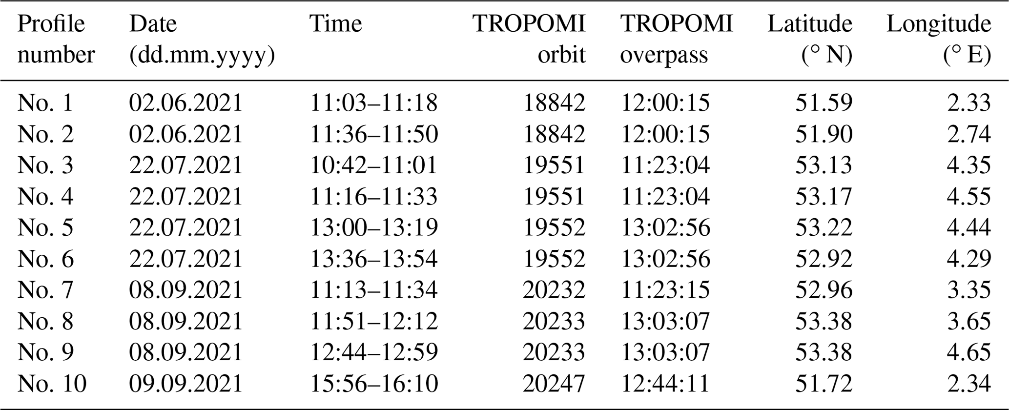
Table 3 Overview of vertical profile flights taken during this campaign. Times are in UTC. Latitude and longitude columns indicate the center of the profile.

3.1.2 Plume NO_x-to-NO₂ conversion

The NO₂ measurement values are taken from the differences between the Ecotech sensor's NO_x and NO concentrations. However, near the edges of plumes, we find unrealistically high or even negative NO₂ concentrations due to the small time delay between the NO_x and NO sampling in the Ecotech instrument, as mentioned in Sect. 2.2 and illustrated in Fig. 3 (right panel). When the aircraft samples background air, the NO₂ values inferred from NO_x − NO are still reliable in spite of the small delay. But when the aircraft samples the plume, we can not necessarily rely on NO_x − NO and instead convert the NO_x concentration measurements into NO₂ concentrations via local NO₂ : NO_x ratios simulated with the PARANOX plume chemistry model which has been used before by Vinken et al. (2011) for ship plume modeling. PARANOX NO₂ : NO_x ratios depend strongly on the age of the plume, as NO_x in the early stages after emissions is mostly present as NO, but the NO₂ portion typically increases to 0.45 within some 15–30 min after emission following entrainment of O₃ and subsequent NO₂ formation via the NO + O₃ reaction in the plume. More details on PARANOX can be found in Sect. S2.

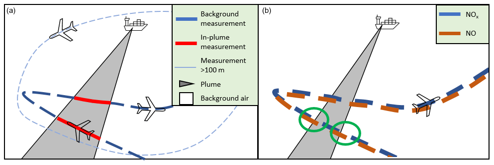
Figure 3 Sketches of profile flights visualizing the corrections. (a) The gray area indicates the part of the 2D plane covered by a plume and the thick line the aircraft measurements in the polluted layer, with red showing in-plume measurements and blue indicating background sampling. The mismatch between the fraction of time spent in-plume and the fraction of the area covered by the plume is apparent. (b) The blue dashes indicate intervals of measuring NO_x, while the orange dashes indicate NO-intervals. For the situations highlighted by the green circles NO is measured partly in-plume, while NO_x is measured fully in-plume (left circle) or out-of-plume (right). This will lead to negative or extremely high NO₂ values, respectively.

3.1.3 Zero-level offset calibration

The Ecotech sensor is capable of detecting clear in-plume NO₂ enhancements of several parts per billion, but since near-zero, background air NO₂ levels differed by a few parts per billion between flights on different days, we re-calibrated the aircraft NO₂ concentrations to ensure that the measured near-zero NO₂ levels at altitudes above 250 m were on average consistent with NO₂ values from the CAMS simulations. The calibration offset is applied as an additive correction to the entire profile, and its value is consistent for multiple profiles measured on the same day, as anticipated from the daily calibration routine executed prior to flight. The calibration offsets vary between 0 and 4 ppb between the different days, and we assume an uncertainty of the bias correction of 0.5 ppb. Using only values above 500 m for the offset calculation leads to slightly different offsets that fall within the assumed uncertainty range. For a more detailed description of the three corrections, see Sect. S3.

3.2 Observed vertical NO₂ profiles

We now present the vertical NO₂ profiles obtained from the BN2 aircraft measurements over the North Sea following the procedure sketched in Sect. 3.1. Each of these vertical NO₂ profiles is spatially representative of the spatial scale of a TROPOMI pixel. For the time and location of the profiles taken, see Table 3. Aircraft NO₂ measurements were aggregated in 50 m altitude bins, where the reported altitude is the mean of the lower and upper boundary of each bin.

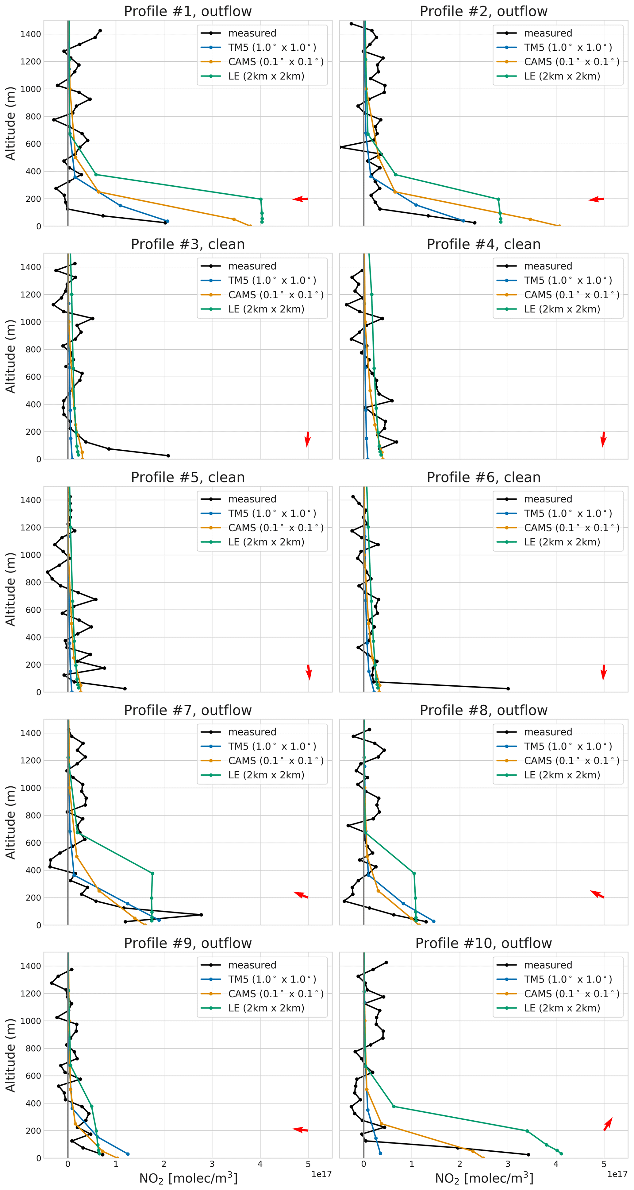
Figure 4 Profiles of all flights and coinciding TM5, CAMS ensemble mean and LOTOS-EUROS profiles. The red arrows indicate the mean measured wind direction during the profile flights. The indicators “outflow” and “clean” in the subtitles follow the classification in Sect. 3.2.

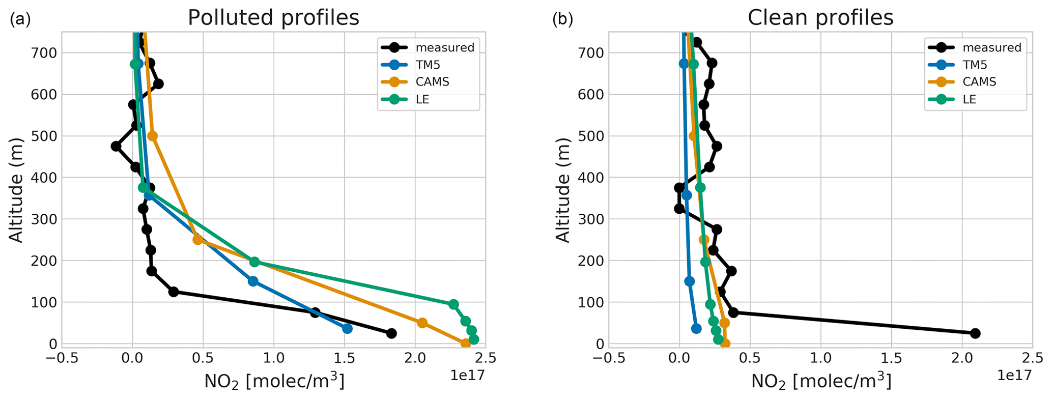
Figure 5 Mean aircraft-measured profiles and coinciding TM5, CAMS ensemble mean and LOTOS-EUROS profiles for land outflow (a: profiles 1, 2, 7, 8, 9, 10) and clean conditions with northerly winds (b: profiles 3, 4, 5, 6).

The aircraft data show the highest NO₂ concentrations close to the sea surface, strongly decreasing within the lowest 100 m (Fig. 1). This is in agreement with the CO₂ profiles shown in Sect. S5. To better understand the emission sources and physical transport processes leading to the observed profile shapes, we analyze simulations over the campaign period from the TM5-MP, CAMS and LOTOS-EUROS models (see Sect. 2.3). The mean simulated NO₂ profiles coinciding with the aircraft flights show NO₂ pollution up to 200 m and above (Fig. 1). In the following, we will investigate the roles of model vertical mixing, emission strength and transport of pollution from elsewhere as possible explanations for the mismatch between the simulations and observations. For that we need to study the NO₂ profiles according to their distinct meteorological circumstances. Figure 4 shows the individual measured and modeled profiles with the numbering consistent with Table 3. For uncorrected profiles and the uncertainty estimates, see Fig. S4. Meteorological conditions such as mean wind direction reveal that vertical profiles have been collected for two distinctly different types of situations over the North Sea: one with outflow of possibly polluted air from the Low Countries over the North Sea and one under pristine conditions with wind from the north and low background NO₂ concentrations. Hereafter we classify these profiles as “land outflow” and “clean” (see Fig. 5). A more complete description of the general chemical and meteorological conditions during each flight can be found in Sect. S1.

3.2.1 NO₂ profiles during land outflow – profiles 1, 2, 7, 8, 9 and 10

Figure 6 shows the observed and simulated NO₂ in a situation of outflow from continental Europe. We see that the profile (indicated by the blue circle) was indeed sampled under conditions of pollution outflow from land. The corresponding profiles for all outflow cases in Fig. 4 show pollution close to the sea surface (see also the left panel of Fig. 5). While the aircraft-measured NO₂ is enhanced only in the lowest 100 m (for the exception of profile 7 see below), the models – especially LOTOS-EUROS – show elevated NO₂ usually up to 200 m and above. This gives an overestimation in the total NO₂ in the column. The measured and modeled potential temperature profiles (Fig. S2) show a cold sea surface with a strong gradient in the lowest 400 m, hinting at a strong stratification. Together with moderate wind speeds this indicates stable conditions with limited vertical mixing.

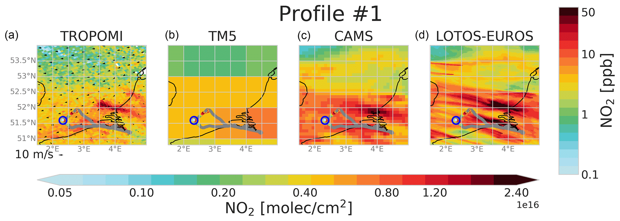
Figure 6 NO₂ columns (indicated by the bottom color bar) as seen by TROPOMI and several model products for the time of the first profile measurement. The aircraft measurements are overlaid in gray for flights above 200 m and in color for those below, as indicated by the color bar on the right. Wind speed and direction at 10 m from ERA5 are indicated by the arrows in panel (a).

TM5 grid cells are very large and contain a mixture of land and sea surfaces, as can be seen in Fig. 6. This means that emissions within the cell can originate from land-based sources as well as ships. Likewise, boundary layer dynamics are a mix of sea and land characteristics. Nonetheless, TM5 profiles show only slightly less NO₂ in the lowest layer than the LOTOS-EUROS, CAMS and the measured profiles for outflow cases (see Fig. 5, left). Overall, the coarse TM5 columns show reasonable agreement with TROPOMI-retrieved columns during outflow conditions with the exception of profile 10 (see Figs. 4 and S5).

On the other hand, the higher horizontal resolution in CAMS and LOTOS-EUROS allows the separation of sea and land NO_x contributions. The resulting columns show massive outflow of NO₂ from land, and we see plume-like structures from the region of Antwerp and Rotterdam in CAMS, LOTOS-EUROS and TROPOMI. Aircraft profile 1 shown in Fig. 6 was taken within the outflow of Antwerp pollution. LOTOS-EUROS and, to a lesser degree, also CAMS show overestimated NO₂ columns compared to TM5 and TROPOMI. This is in line with the observed profiles shown in Figs. 4 and 5: while surface NO₂ levels in LOTOS-EUROS and CAMS are in reasonable agreement with observations overall, the polluted layer is significantly deeper than in the observations, leading to a high bias in LOTOS-EUROS and CAMS NO₂ columns in these outflow cases. Additionally, CAMS and LOTOS-EUROS show two strong emission plumes in the North Sea (e.g., around 53.3^∘ N, 2.5^∘ E) which are not visible in TROPOMI or TM5. These likely originate from gas platforms, but the missing plumes in the TROPOMI observations point at large overestimations of the emission strength in the CAMS inventory (≈ 0.2 kg s⁻¹ for these two sources). TROPOMI and modeled NO₂ columns during the other profile flights can be found in Sect. S4.

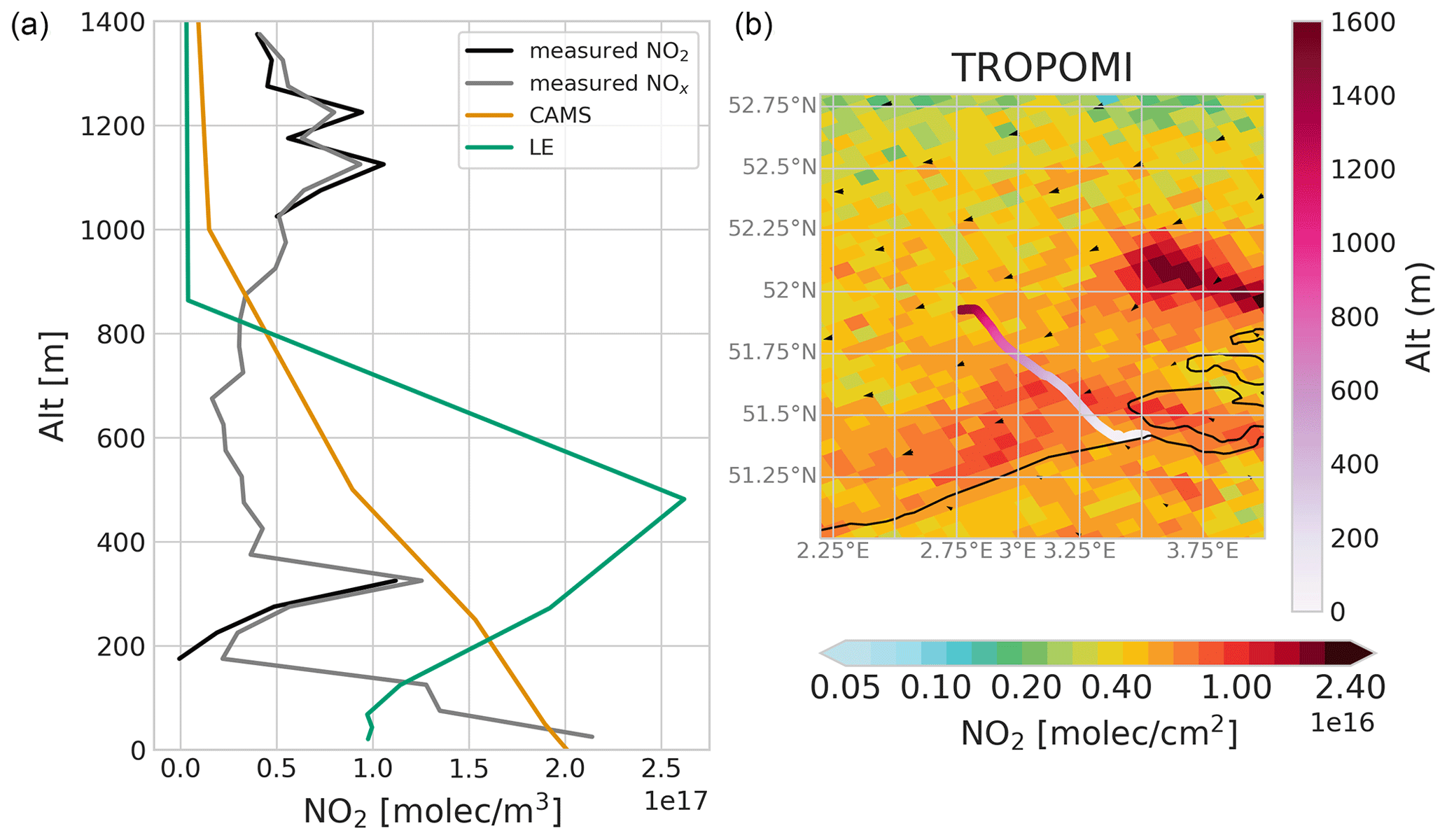
Figure 7 (a) Measured and modeled vertical distribution of NO₂ along the flight path indicated in panel (b). This is not a vertical profile in the strict sense, as the sampling took place over a ≈ 70 km horizontal extent. During part of the flight the airplane instrumentation was operating in a different mode so that no NO₂ data are available. However, NO_x (gray) was sampled throughout the whole flight and indicates a thin pollution layer between 300 and 400 m.

A special case is profile 7 on 8 September. This is the only profile with clearly enhanced NO₂ above 100 m (see also Fig. S6 for the CO₂ profile). In fact, the profile agrees reasonably well with TM5 and CAMS data, whereas LOTOS-EUROS again shows a mixing layer that is too deep and too much NO₂ in the column. This enhanced NO₂ observed between 100 and 300 m altitude might be caused by polluted air masses originating from the Netherlands and transported over sea while rising above the stable surface layer. This hypothesis is supported by parts of the flight on 2 June, when enhanced NO₂ was observed at an altitude of 300 m descending towards Antwerp airport into the land outflow after taking profile 2. A vertical profile for this part of the flight and the flight path can be seen in Fig. 7. The observed NO₂ layer at 300 m is also present in the co-sampled LOTOS-EUROS profile (as a thicker NO₂ layer around 500 m) but not in CAMS. These findings also demonstrate that the aircraft instrumentation is able not only to detect high NO₂ values in fresh plumes but also to capture diluted NO₂ pollution from land. Additionally, this suggests that at least for profile 2 (which was sampled right before) enhanced NO₂ seen at 200 m in the models is unlikely to be caused by land emissions, as pollution originating from land would be expected higher in the atmosphere. Finally, this indicates that land outflow often observed by TROPOMI over the North Sea can be located in higher atmospheric layers where TROPOMI has a higher sensitivity (see Sect. 4), thus possibly masking the low-level NO₂ from ships.

In summary, all models successfully simulate the occurrence of outflow and match the observed surface pollution reasonably well, but especially CAMS and LOTOS-EUROS overestimate the (vertically integrated) amount of NO₂. From our observations it remains unclear whether the high NO₂ in LOTOS-EUROS and CAMS is caused by overestimations in land-based emissions, timing of the emissions in the models, advection, NO₂ lifetimes that are too long or vertical mixing. Similar to the other models, TM5 shows NO₂ that is too high at 200 m and above, hinting at uncertainties in the vertical mixing. The low surface pollution of TM5 in profile 10 likely showcases the limitations of a coarse resolution. The very shallow pollution layer visible in the NO₂ measurements is also visible in the uncorrected and simultaneously measured CO₂ data (see Fig. S6) and is therefore unlikely to result from the non-simultaneous measurement of NO_x species and our corrections.

3.2.2 NO₂ profiles during clean conditions – profiles 3, 4, 5 and 6

Figure 8 shows the observed and simulated NO₂ in a situation without outflow from continental Europe. Profiles 3 to 6 have all been taken on the same day, 22 July 2021. On this day northern winds were prevailing, transporting clean air into the North Sea, resulting in low NO₂ columns as observed by TROPOMI in Figs. 8 and S1. The potential temperature profile on 22 July 2021 (see Fig. S2) indicates a well-mixed marine boundary layer of 800 m depth. All modeled NO₂ profiles show little pollution at the surface, and NO₂ concentrations are slightly decreasing towards higher altitudes. While the profiles were taken right above the shipping lane, marked by the blue circle in Fig. 8, in CAMS and LOTOS-EUROS the shipping pollution can be seen south of the profile, caused by the northerly winds. Again, TM5 shows less NO₂ compared to the other models (see Figs. 5, 8 and S5).

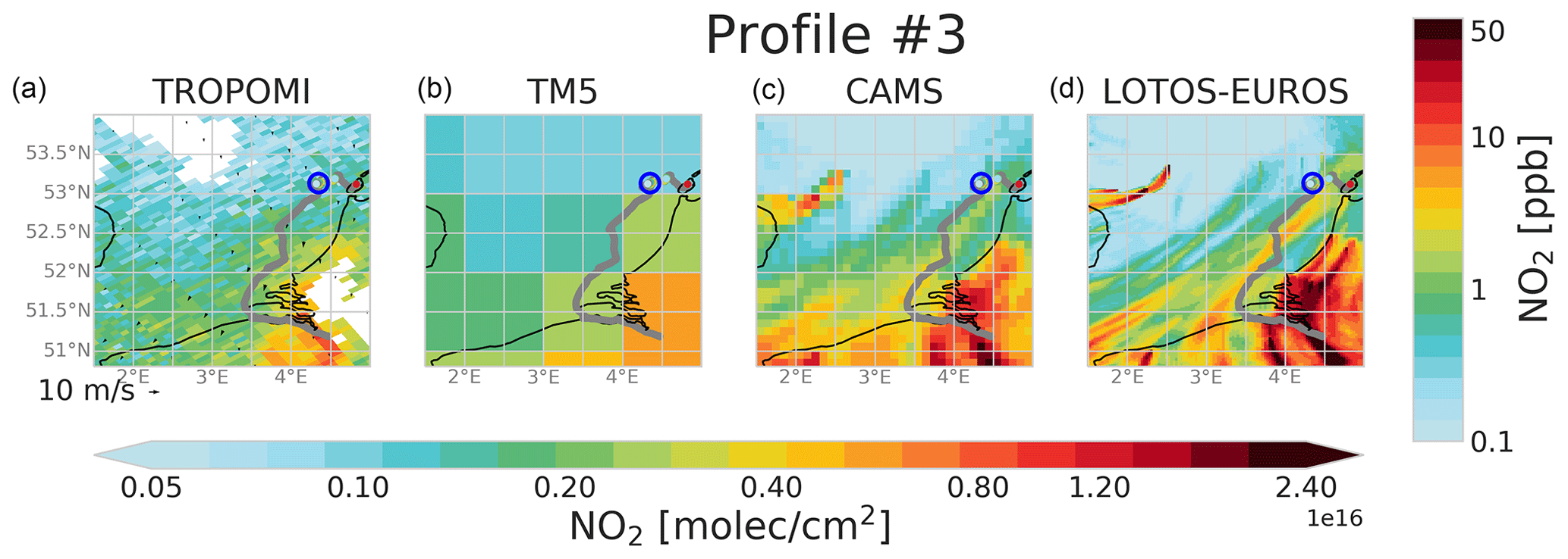
Figure 8 As Fig. 6 but now for the third profile. Profile 4 is taken in collocation with the same TROPOMI orbit, and its location is shown in Fig. S5.

The observed profiles 4 and 5 (see Fig. 4) agree reasonably well with the models, showing little NO₂ enhancement close to the sea surface. On the other hand, profiles 3 and 6 show strong NO₂ enhancements in the lowest 50 m, in contrast to the models. This is driven by exceptionally high NO_x concentration measured in ship plumes (> 250 ppb NO_x for profile 3). In fact, a Monte Carlo approach (see Sect. S3 and Fig. S4, leading to a more multi-profile-average “in plume” NO₂ concentration) shows very similar surface NO₂ values of ≈ 1.5 × 10¹⁷ molec. m⁻³ for all four flights on that day. This shows the presence of ship plumes in all four profiles, while in two cases either the plume was not captured well due to the temporal sampling of the Ecotech sensor or the ships in profiles 4 and 5 were emitting significantly less.

The mean clean profile in the right panel of Fig. 5 shows that none of the models captures the clear enhancement in the lowest 50 m due to NO_x emissions from ships. The ship NO_x emissions – while captured by the aircraft – are spatially diluted over the area of the model grid cell, especially for the coarse TM5 model, and throughout the well-mixed boundary layer and are advected with the prevailing wind. Additionally, the models represent ships with averaged, constant emission fluxes in the model grid cells along the ship tracks, whereas in reality a ship might be in a given model grid cell for a short time with a higher emission flux. Therefore, in reality strongly localized emission levels are observed as sharply defined plumes that are not resolved by the chemistry transport models (CTMs). These observations indicate the weakness of temporally and spatially averaged emissions in the models which fail to capture high pollution levels in the vicinity of strong and moving emitters. Overall, the models seem to underestimate the influence of ship emissions likely due to temporal and spatial averaging of emissions and instant dilution thereof in the grid cell.

4 Validation of TROPOMI NO₂ over the North Sea

4.1 Recalculate AMFs

With the observed vertical NO₂ profiles we can calculate a modified TROPOMI NO₂ column, replacing the coarse TM5 a priori in the retrieval with aircraft-measurement-based vertical profiles. As the measured NO₂ profiles only extend to 1400 m, we use TM5 profiles to fill the gap to the tropopause. The combined aircraft–TM5 profiles have then been interpolated and sampled according to the TM5-MP vertical levels. The adjusted tropospheric AMF M_trop,ADJ can be calculated using the AMF from the a priori M_trop,TM5, the averaging kernels of layer l A_trop,l provided in the TROPOMI files and the NO₂ column density x_l,meas of layer l from the aircraft data as

$$\begin{array}{}\text{(1)}& M_{\mathrm{trop},\mathrm{ADJ}}=M_{\mathrm{trop},\mathrm{TM}\mathrm{5}}\times {\displaystyle \frac{{\sum }_{l=\mathrm{1}}^L{A}_{\mathrm{trop},l}{x}_{l,\mathrm{meas}}}{{\sum }_{l=\mathrm{1}}^L{x}_{l,\mathrm{meas}}}},\end{array}$$

where L is the highest TM5 layer below the tropopause. Replacing the a priori with the measured NO₂ profiles and recalculating the AMFs are explicitly advised in the TROPOMI NO₂ documentation (Eskes and van Geffen, 2021) and have been done to improve satellite observations and validations previously (Visser et al., 2019; Douros et al., 2023). The adjusted vertical, tropospheric column can then be calculated as $N_{\mathrm{v},\mathrm{trop},\mathrm{ADJ}}=N_{\mathrm{s}}/M_{\mathrm{trop},\mathrm{ADJ}}$.

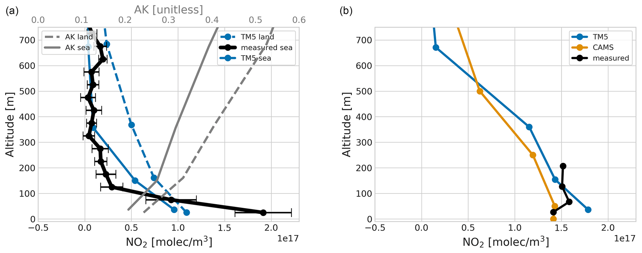
Figure 9 (a) The solid blue line shows mean TM5 profiles coinciding with the aircraft profiles (black). The dashed blue line shows simultaneous TM5 NO₂ profiles at the Cabauw tower in the Netherlands. Additionally, the mean TROPOMI averaging kernel profiles for land (sampled for all TROPOMI pixels within 51.90–52.04^∘ N and 4.86–5.00^∘ E) and sea (co-sampled with the aircraft profile measurements) are shown. Panel (b) shows mean measured (black) and modeled (TM5 in blue and CAMS in yellow) profiles at the Cabauw tower in the Netherlands for 6 cloud-free days in September–October 2019 during the TROLIX-19 campaign (Sullivan et al., 2022).

NO₂ concentrations in TM5 that are too low close to the surface are expected to lead to a negative bias in the TROPOMI NO₂ retrievals since the sensitivity to NO₂ close to the sea surface is generally small as indicated by the averaging kernel (see Fig. 9). The shallow boundary layer depth over sea in combination with the low surface albedo values (≈ 0.04) emphasizes the difficulty in detecting air pollution over sea with satellite remote sensing despite the high signal-to-noise ratio and resolution of TROPOMI NO₂.

4.2 Tropospheric columns

We compare vertical tropospheric columns of NO₂ retrieved by TROPOMI (operational, PAL and CAMS), as well as measured columns. Lastly, we add the new product TROPOMI_ADJ, which includes a re-calculation of the AMFs and vertical tropospheric NO₂ columns using the measured profiles following Sect. 4.1.

Table 4 Tropospheric NO₂ columns measured by the aircraft and different TROPOMI products. For TROPOMI_ADJ, the values in the bracket give the average of the lower and upper estimates based on the uncertainties shown in Fig. S3.

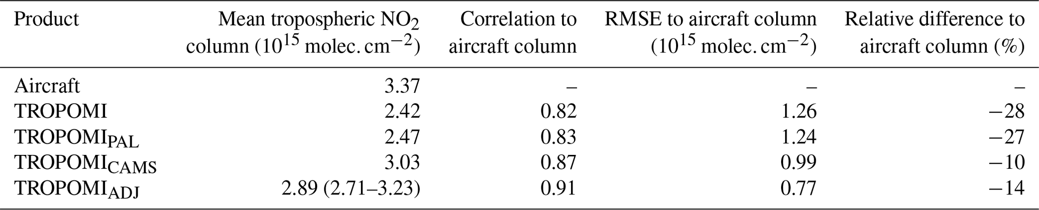
Table 4 shows the mean column densities of all datasets mentioned above, as well as their Pearson correlation coefficient and root mean squared error (RMSE) against the aircraft data. The 10 aircraft-measured NO₂ column densities averaged at 3.37 × 10¹⁵ molec. cm⁻². This is significantly higher than the coinciding operational TROPOMI (2.42 × 10¹⁵ molec. cm⁻²) and TROPOMI_PAL (2.47 × 10¹⁵ molec. cm⁻²) data. Using the re-calculated AMFs an average column density $N_{\mathrm{v},\mathrm{trop},\mathrm{adj}}$ of 2.89 (2.71–3.23) × 10¹⁵ molec. cm⁻² is determined. This is ≈ 20 % (12 %–33 %) higher than the TROPOMI products and brings the satellite retrievals closer to the columns determined from the aircraft measurements, showing a significant negative bias in operational TROPOMI NO₂ columns. The TROPOMI_CAMS dataset (see Sect. 2.1) is closer to the measured columns at mean columns of 3.03 × 10¹⁵ molec. cm⁻². It should be noted that CAMS NO₂ columns (see Figs. 6, 8 and S5) are systematically higher compared to measurements and TM5. TROPOMI_CAMS and TROPOMI_ADJ also show an increased Pearson correlation coefficient compared to the aircraft columns of 0.87 and 0.91, respectively, compared to 0.82 of the operational product. Lastly, the RMSE of the TROPOMI columns towards the aircraft columns reduces going from the operational (1.26 × 10¹⁵ molec. cm⁻²) to TROPOMI_CAMS (0.99 × 10¹⁵ molec. cm⁻²) data and is smallest for the aircraft-adjusted columns at 0.77 × 10¹⁵ molec. cm⁻².

Given the large uncertainty and corrections involved at the NO₂ concentrations close to the sea surface, the sensitivity of the recalculated AMFs to that value was tested. A 20 % change in the NO₂ number density leads to a change in AMF of less than 5 %, and even a change of 50 % in surface level NO₂ changes the AMF only by 10 %. This supports the finding of a negative bias caused by the a priori profile, as the differences in AMFs can not be explained by the surface level NO₂ alone.

4.3 The land–sea contrast in TROPOMI NO₂ retrieval

As a contrasting case, Fig. 9 compares the sea NO₂ profiles to NO₂ profiles during the TROpomi vaLIdation eXperiment in 2019 (TROLIX-19) (Sullivan et al., 2022) over the Netherlands (51.97^∘ N, 4.93^∘ E). The left panel shows mean TM5 NO₂ and averaging kernel profiles over land and sea at the time of the aircraft measurements, as well as the mean aircraft-measured profiles. While modeled surface pollution levels over land are on average close to those over sea, the boundary layer is significantly more evolved with elevated pollution levels in the models reaching 400 m and above. At the same time, the averaging kernel over sea is smaller compared to land throughout the entire boundary layer. The right part of the same figure shows midday NO₂ concentrations measured at Cabauw tower, as well as coinciding TM5 and CAMS profiles co-sampled during the TROLIX-19 campaign which took place at a different time than the aircraft measurements but under similar meteorological conditions. No measured profile data are available at Cabauw for the days of the aircraft campaign. The measurements confirm a well-mixed lowest 200 m, in contrast to the presented profiles over sea. Even if the models would overestimate vertical mixing over land, the higher mixed layer over land would lead to a smaller relative difference between modeled NO₂ concentration and observations compared to over sea. This – together with the lower surface albedo (< 0.04 for the North Sea vs. 0.05 for land) causing a lower sensitivity to NO₂ close to the surface – emphasizes the challenge of accurate satellite retrieval of NO₂ over sea compared to over land. For more details, see Sect. S6. Overall, we find on average 20 % lower tropospheric AMFs over the North Sea compared to land given similar overall retrieval conditions.

5 Discussion

We evaluated the TROPOMI tropospheric vertical NO₂ column retrieval over the North Sea. For this, we measured 10 vertical NO₂ profiles in the immediate vicinity of ships emitting air pollutants coinciding with the TROPOMI overpass, compared them to modeled profiles and studied the impact of a priori profiles on the TROPOMI NO₂ column retrieval.

Flying down to below 30 m above the sea surface allowed us to fully capture ship plumes and NO₂ pollution over the North Sea. While our measurements suffer from the indirect measurement of NO₂, the horizontal zigzag patterns and applied corrections lead to profiles that are truly representative at the time and scale of a TROPOMI pixel.

Our measurements strongly hint at systematic negative bias in TROPOMI NO₂ columns over the polluted North Sea. Using the aircraft profiles to recalculate the AMFs and tropospheric NO₂ columns, the TROPOMI columns are ≈ 20 % (12 %–33 %) larger on average compared to TROPOMI_PAL data using TM5 for a priori profiles. This is in agreement with earlier studies (Douros et al., 2023) for point sources. The vertical profile measurements over the North Sea reveal a very shallow boundary layer of 100–150 m above sea level, where the averaging kernel is the smallest. With one exception our measurements show no significant pollution above 150 m. This finding is supported by co-sampled CO₂ profiles presented in Sect. S5. The low pollution layer is in contrast to model profiles and could be attributed to an overestimated vertical mixing in the models compared to observations on 4 summer days in 2021. The mixing schemes for vertical transport in the boundary layer used in TM5 (Williams et al., 2017; Holtslag and Boville, 1993) are known to overestimate vertical mixing for stable conditions (Köhler et al., 2011) which prevailed during several of the campaign days (see Sect. 3.2). The updated K diffusion based on the Monin–Obukhov length used in LOTOS-EUROS (ECMWF, 2015) is expected to result in more shallow stable boundary layers. However, we still find a high bias in LOTOS-EUROS in the mixed layer height. Hints towards uncertainties in the vertical mixing of the LOTOS-EUROS can also be found in Escudero et al. (2019), who show a positive bias in boundary layer height (BLH) over Madrid in summer, as well as overestimated vertical mixing in the boundary layer using the LOTOS-EUROS mixed layer scheme. Additionally, they find more gradual vertical mixing and a better correlation of ozone surface measurements when increasing the number of vertical layers. Likewise, Skoulidou et al. (2021) connect underestimated surface NO₂ levels in Athens to problems in the temporal evolution of the BLH in LOTOS-EUROS, which is taken from the ECMWF operational weather analysis.

The very shallow mixed layer observed during the flights is in agreement with the observed strong gradient in potential temperature and indicates stable conditions. The reasons the models fail to reproduce the shallow mixed layer over the North Sea remain unclear and need further study.

Next to the overestimated mixing, the TM5 profiles during clean conditions show less pollution close to the surface than the aircraft data and the other model simulations. This is likely an effect of the coarse TM5 resolution of 1^∘ × 1^∘, where ship emissions are smeared out over a larger area and time. The exaggerated vertical mixing and underestimation of the lowest part of the profile in TM5 lead to high-biased AMFs which in turn decreases the vertical column density via $N_{\mathrm{v}}=N_{\mathrm{s}}/M$. While the higher spatial resolutions of CAMS and LOTOS-EUROS increase the surface level NO₂ (in fact, for 8 out of 10 profiles, the surface pollution in these model products agrees reasonably well with observations), they overestimated pollution layer height, giving a substantial overestimation of the total NO₂ in the columns. This may be caused by overestimated NO_x emissions, their timing in the models, exaggerated advection or NO_x lifetimes that are too long, and it shows that increased horizontal resolution does not necessarily give more accurate profile shapes. While TROPOMI columns using CAMS profiles as a priori are higher and show better correlation and lower RMSE to the aircraft columns than using TM5, this is caused rather by the higher NO₂ column than by a correct profile shape. The TROPOMI_CAMS product, essentially, demonstrates improved agreement with the aircraft column compared to the operational product. However, using the aircraft profiles in the AMF calculation exhibits the highest correlation and lowest RMSE.

Furthermore, we conclude that TM5, CAMS and LOTOS-EUROS are unable to fully capture the spatially and temporally confined ship emissions over sea and that the pollution levels as a result of land outflow dominate the model results. This is supported by profiles 3–6, which were measured in clean conditions without land outflow. Observed and modeled temperature profiles indicate a well-mixed atmosphere up to ≈ 800 m, and we see little NO₂ enhancement in all model products, while we observe strong enhancements in profiles 3 and 6 as discussed before. The observed enhancements can be directly linked to fresh ship plumes that are shown to be vertically confined to the lowest 50 m and are not present in the models. Better results can be expected with plume-resolving models, incorporating ship plumes using AIS and ship-specific data for their location and emission strength (e.g., from Jalkanen et al., 2016) or from a climatology of representative NO₂ profiles observed over shipping routes. The presented profiles can be the starting point for such a climatology.

More validation flights over polluted sea are desirable, especially spanning different locations, seasons and meteorological conditions as this study was limited to 4 d over the North Sea in summer. A total of 6 out of the 10 profiles (on 3 of the 4 d) were taken under land outflow conditions. Being close to major polluting areas in the British Islands and northwestern Europe, land outflow happens frequently, and we therefore expect these sampling conditions to be representative of the North Sea. While this study presents a cost-efficient way of measuring NO₂ profiles utilizing an aircraft already equipped for emission monitoring, direct NO₂ measurements with a temporal resolution of 1 Hz or higher and higher accuracy could have reduced postprocessing and uncertainties. Better calibration, a more sensitive sensor and expanding the flights to higher altitudes can further reduce the dependence on model simulations.

Overall, this study shows the bias arising from using modeled and uncertain a priori profiles. This is true especially over sea where the boundary layer is less developed than over land and the surface is darker. The observed negative bias in TROPOMI has important implications for the application of TROPOMI NO₂ columns for ship emission monitoring. As advised in Eskes and van Geffen (2021) the recalculation of AMFs using more realistic a priori profiles is beneficial.

6 Conclusion

This study clearly shows the need for additional evaluation of vertical NO₂ profiles over sea for both model and TROPOMI validation while providing a blueprint for such an analysis. We present 10 vertical profiles of NO₂ over the North Sea in summer, which – due to the low-altitude sampling (< 30 m) and the location over busy shipping routes – present a unique opportunity to evaluate TROPOMI vertical NO₂ columns and model profiles (TM5, CAMS and LOTOS-EUROS) that was previously missing from the literature.

We find that on average the coarse resolution of TM5 leads to NO₂ concentrations that are too low near the surface while overestimating NO₂ above 100 m. The higher model resolution of CAMS and LOTOS-EUROS results in more accurate surface NO₂ values, while at the same time vertical mixing is exaggerated compared to our observations. Additionally, CAMS and LOTOS-EUROS vertical NO₂ columns are too high compared to aircraft and TROPOMI data.

Furthermore, the comparison between observed and modeled vertical NO₂ profiles, along with the examination of TROPOMI averaging kernels over land and sea, stresses the significant challenges involved in accurately retrieving satellite NO₂ columns over sea, where vertical sensitivity to NO₂ is 20 % lower than over land because of lower surface albedo and confinement of NO₂ pollution in a thin marine boundary layer.

When replacing the TM5 a priori profiles with the aircraft-measured NO₂ profiles in the TROPOMI AMF calculation, we find a significant increase in the retrieved vertical NO₂ columns of ≈ 20 % (12 %–33 %), showing substantially improved agreement with aircraft-measured columns. Our findings align with previous studies (e.g., by Douros et al., 2023; Pseftogkas et al., 2022; Lorente et al., 2017), highlighting the importance of precise vertical a priori profiles for satellite-based trace-gas retrieval.