Daily satellite-based sunshine duration estimates over Brazil: validation and intercomparison

The broad geographical coverage and high temporal and spatial resolution of geostationary satellite data provide an excellent opportunity to collect information on variables whose spatial distribution and temporal variability are not adequately represented by in situ networks. This study focuses on assessing the effectiveness of two geostationary satellite-based sunshine duration (SDU) datasets over Brazil, given the relevance of SDU to various fields, such as agriculture and the energy sector, to ensure reliable SDU data over the country. The analyzed datasets are the operational products provided by the Satellite Application Facility on Climate Monitoring (CMSAF) that uses data achieved with the Meteorological Satellite (Meteosat) series and by the Satellite and Meteorological Sensors Division of the National Institute for Space Research (DISSM–INPE) that employs Geostationary Operational Environmental Satellite (GOES) data. The analyzed period ranges from September 2013 to December 2017. The mean bias error (MBE), mean absolute error (MAE), root mean squared error (RMSE), correlation coefficient (r), and scatterplots between satellite products and in situ daily SDU measurements provided by the National Institute of Meteorology (INMET) were used to access the performance of the products. They were calculated on a monthly basis and grouped into climate regions. The statistical parameters exhibited a uniform spatial distribution, indicating homogeneity within a given region. Except for the tropical northeast oriental (TNO) region, there were no significant seasonal dependencies observed. The MBE values for both satellite products were generally low across most regions in Brazil, mainly between 0 and 1 h. The correlation coefficient (r) results indicated a strong agreement between the estimated values and the observed data, with an overall r value exceeding 0.8. Nevertheless, there were notable discrepancies in specific areas. The CMSAF product showed a tendency to overestimate observations in the TNO region, with the MBE consistently exceeding 1 h for all months, while the DISSM product exhibited a negative gradient of the MBE values in the west–east direction in the northern portion of Brazil. The scatterplots for the TNO region revealed that the underestimation pattern observed in the DISSM product was influenced by the sky condition, with more accurate estimations observed under cloudy skies. Additional analysis suggested that the biases observed might be attributed to the misrepresentation of clear-sky reflectance. In the case of the CMSAF product, the overestimation tendency observed in the TNO region appeared to be a result of systematic underestimation of the effective cloud albedo. The findings indicated that both satellite-based SDU products generally exhibited good agreement with the ground observations across Brazil, although their performance varied across different regions and seasons. The analyzed operational satellite products present a reliable source of data to several applications, which is an asset due to its high spatial resolution and low time latency.

1 Introduction

Sunshine duration (SDU) is conceptually defined as the total hours of sunlight reaching the Earth's surface directly from the Sun. With the advance of technology and measurement instruments, it was formally defined as the sum of the periods in which direct solar irradiance reaches or exceeds 120 W m⁻² (WMO, 2008). Along with precipitation and surface air temperature, it is one of the most important parameters in climate monitoring (Kothe et al., 2013). In a given area, the amount of sunshine received is the major factor determining the local climate (Bertrand et al., 2013).

The SDU importance has been known for a long time, and its first measurements date back to the 19th century. In fact, there are time series of SDU measurements of as long as 100 years that have been accumulated at networks all over the world. SDU data are relevant for a number applications, such as yield planning in agriculture (Rao et al., 1998; Huang et al., 2012; Wang et al., 2015), analysis of the thermal loads and sunshine duration on buildings (Shao, 1990), input parameters in soil water balance models (Warnant et al., 1994), and even research on human health (McGrath et al., 2002; Nastos and Matzarakis, 2006; Keller et al., 2019). Akinoglu (2008) stated that SDU data are the best long-term, trustworthy, and readily available measurements to estimate the surface solar irradiation, due to the linear relationship between these variables, as described by Angstrom (1924).

Based on that, the necessity of SDU records is clear. However, there is a relatively small number of stations that measure it. Overall, networks of SDU are sparse and insufficient to cover large areas (Kandirmaz and Kaba, 2014). In Brazil, the National Institute of Meteorology (INMET) currently operates a network with 245 stations; moreover, it provides SDU time series from 85 other sites that are no longer operational. The effort to maintain this network is essential to provide reliable SDU records for climate studies. Nonetheless, compared to the temperature or precipitation networks with thousands of stations, the SDU current network seems inadequate to cover the large Brazilian territory.

Along with that, although meteorological station measurements are point-based observations (Zhu et al., 2020), the SDU in the vicinity has to be obtained through interpolation techniques. Therefore, the accuracy of the method strongly relies upon the number and spatial distribution of meteorological stations. Generally, the station distribution is heterogeneous, with most of them being near cities; for several reasons, extensive areas remain without records. For instance, it can be observed in Brazil, where some regions in the north have very few stations, while the southern and southeastern regions present a denser network. Consequently, the resulting interpolated field is usually poor for representing the temporal and spatial SDU variability characteristics (Wu et al., 2016).

Geostationary satellites perform measurements with high spatial and temporal resolution and cover large areas, so their data can be used as an alternative to estimate SDU. The literature on the subject provide some proposed methods to accomplish this goal. Given the fact that clouds are primarily responsible for SDU changes, several methods to derive SDU rely on them. Different techniques have been considered, such as an SDU estimate based on the cloud cover index (Kandirmaz, 2006; Ceballos and Rodrigues, 2008; Shamim et al., 2012) and from satellite-derived cloud-type products (Good, 2010; Wu et al., 2016; Zhu et al., 2020). Another approach is given by Kothe et al. (2017), in which the SDU is calculated based on direct normal radiation threshold, using data from the Meteorological Satellite (Meteosat) series operated by the European Organisation for the Exploitation of Meteorological Satellites (EUMETSAT). Currently, this approach has been considered to be one of the most advanced remote sensing tools to estimate the SDU and is operational at the Satellite Application Facility on Climate Monitoring (CMSAF).

In South America, Ceballos and Rodrigues (2008) proposed a SDU estimation method based on Geostationary Operational Environmental Satellite (GOES) data. It is operational at the Satellite and Meteorological Sensors Division of the National Institute for Space Research (DISSM–INPE). This method (hereafter DISSM method) was validated by the authors, using in situ measurements from the cities of São Paulo and Fortaleza, and their results indicated a good agreement between the estimates and the observed data. Thereafter, Porfirio (2012) extended the validation of the INPE method for northeastern Brazil, using records from 53 stations for 2008, showing a good performance of the method. However, the climatic characteristics of that region are not representative of the whole country.

In addition, the satellite-derived SDU dataset from CMSAF (hereafter CMSAF method) also provides estimates over Brazilian territory. However, the accuracy of the product was only evaluated for the monthly sums and a few stations (Kothe et al., 2017). Therefore, it is still necessary to have a deep validation of the daily SDU estimates based on satellite data over Brazil.

In this study, we aimed to evaluate the performance of two operational SDU estimate products over Brazil and intercompare their results. The following scientific questions were addressed:

• 1.

  Are those products a good fit for the in situ measurements?

• 2.

  Are there regions in which one of the products performs better than the others?

• 3.

  Are there seasonal variations in the performance?

• 4.

  Could deficiencies in the retrieval be traced to their source?

The paper is structured as follows. Section 2 gives a description of the operational algorithms evaluated, i.e., the DISSM and CMSAF methods. Section 3 describes the ground measurements and statistical metrics used for the validation. Sections 4 and 5 present the obtained results and conclusions, respectively.

2 Satellite-based methods

2.1 DISSM

The DISSM has the mission to produce high-quality satellite products and thus to offer relevant information for different Brazilian sectors. The DISSM was instituted in 2020 and incorporated the former Satellite Division and Environmental Systems (DSA) that has been operational since 1986. The division established itself as a reference that is based on collecting and processing satellite data and satellite product generation for South America (Costa et al., 2018). Among their products are sea surface temperature, severe weather monitoring, precipitation estimation, sunshine duration, and several others (see http://satelite.cptec.inpe.br/, last access: 20 May 2023, and Costa et al., 2018).

To estimate SDU, visible imagery acquired with GOES that is processed by the DISSM is used. From time to time, the GOES platforms are replaced. During the analyzed period in this study (2013–2017), GOES-13 was operational and carried the IMAGER sensor on board. The visible IMAGER channel is centered at 0.65 µm, with a bandwidth of 0.2 µm.

The sensor measures the spectral radiance L_λ ($\mathrm{W}{\mathrm{m}}^{-\mathrm{2}}{\mathrm{sr}}^{-\mathrm{1}}\mathrm{\mu }{\mathrm{m}}^{-\mathrm{1}}$) that represents the mean value in the pixel area. The spectral irradiance at the top of the atmosphere is E_o=μS_λ, where S_λ is the solar irradiance at the normal incidence in this same spectral interval, and μ=cos (SZA) is the cosine of the solar zenith angle. Assuming that the reflected radiance is isotropic, the emergent spectral irradiance at the top of the atmosphere is $E\uparrow =\mathit{\pi }{L}_{\mathit{\lambda }}$, and the reflectance is $R=\frac{E\uparrow }{E_{\mathrm{o}}}$. Operationally, from the satellite visible imagery, the reflectance factor (F) and the planetary reflectance (R) are defined as shown in Eq. (1) (Ceballos and Rodrigues, 2008):

$$\begin{array}{}\text{(1)}& F=\mathit{\pi }{\displaystyle \frac{L_{\mathit{\lambda }}}{S_{\mathit{\lambda }}}};R=f{\displaystyle \frac{F}{\mathit{\mu }}},\end{array}$$

where the factor f is a function correcting the effects of anisotropic reflection (Lubin and Weber, 1995). For the following purposes, f is considered 1 (Ceballos et al., 2004). R is provided by DISSM as a byproduct of the operational processing of the GL1.2 shortwave radiation model (Ceballos et al., 2004).

It is normal to regard the reflectance as a mean value between the cloud reflectance (R_max) and the clear-sky reflectance (R_min) that is weighted by the fraction of the pixel covered by clouds (C), as shown in Eq. (2) (Ceballos et al., 2004).

$$\begin{array}{}\text{(2)}& R=C\cdot R_{max}+(\mathrm{1}-C)\cdot R_{min},\end{array}$$

which leads to an estimate of cloudiness (C) as

$$\begin{array}{}\text{(3)}& C={\displaystyle \frac{R-R_{min}}{R_{max}-R_{min}}}.\end{array}$$

Ceballos et al. (2004) defined the value of R_max as 0.465, which corresponds to the transition between a cumuliform and a stratiform cloud field, and the R_min as 0.09, which is a reasonable value for the continental surface. In the case of $R<R_{min}$, C is set as 0, and if $R>R_{max}$, then C=1. In case of R=0 or when R is marked as invalid (i.e., $R=-\mathrm{99}$), then C is also tagged as invalid.

Next, assuming that the average cloud cover assessed by C is also representative of the relative time of cloud passage over a site inside the pixel (Porfirio and Ceballos, 2017), 1−C corresponds to the relative time of a clear sky. The daily SDU is achieved through Eq. (4), which is similar to the integration via trapezoidal rule (which consists of a numerical method to approximate the integral value):

$$\begin{array}{}\text{(4)}& \begin{array}{rl}\text{SDU}& =\left(\mathrm{1}-C_{\mathrm{1}}\right)+{\displaystyle \frac{\mathrm{\Delta }t}{\mathrm{2}}}[\left(\mathrm{1}-C_{\mathrm{1}}\right)+\mathrm{2}\left(\mathrm{1}-C_{\mathrm{2}}\right)\\ & +\mathrm{2}\left(\mathrm{1}-C_{\mathrm{3}}\right)+\mathrm{2}\left(\mathrm{1}-C_{k-\mathrm{1}}\right)+\left(\mathrm{1}-C_k\right)]+\left(\mathrm{1}-C_k\right),\end{array}\end{array}$$

where C is the cloudiness parameter (described in Eq. 3), C₁ corresponds to the first valid observation for the pixel, the subscript index corresponds to the number of the image within a day, k is the last valid image of the day, and Δt is the time interval between two consecutive images (for the analyzed period, it is usually 30 min).

On average, for a given pixel, 30 images are available for the daily SDU estimate. However, this value can be smaller, and the interval between two consecutive images can be larger than 30 min. The daily SDU for a given day is considered invalid, and is therefore discarded, if there is an interval greater than 3 h (i) between the first image of the day and the sunrise, (ii) between consecutive images, or (iii) between the last image of the day and sunset or if fewer than five images were available for the estimation.

The spatial resolution of the DISSM SDU dataset is 0.04^∘ on a regular latitude–longitude grid of 1800×1800 pixels within latitudes 21.96^∘ N to 50^∘ S and longitudes 100 to 28.04^∘ W, covering the time period from February 2007 to near-real time.

2.2 CMSAF

The EUMETSAT CMSAF was established to contribute to the operational monitoring of the climate and the detection of global climatic changes. With this aim, CMSAF products follow the highest standards and guidelines, as outlined by the Global Climate Observing System (GCOS) for satellite data processing.

The SDU is one of the several products of CMSAF based on Surface Solar Radiation Data Set – Heliosat (SARAH), Edition 2.1 (Pfeifroth et al., 2019). The data record covers the time period from 1983 to near-real time, with a spatial resolution of $\mathrm{0.05}{}^{\circ }\times \mathrm{0.05}{}^{\circ }$. In order to derive the SARAH-2 surface parameters, the Heliosat algorithm is used (Hammer et al., 2003). It provides a continuous dataset of effective cloud albedo and minimizes the impacts of satellite changes and artificial trends, due to the degradation of satellite instruments through an integrated self-calibration parameter (Mueller et al., 2011).

At first, the effective cloud albedo is retrieved by the normalized relation between all-sky and clear-sky reflection in the visible channel of the Meteosat instruments. This parameter is used to derive the cloud index, which is a measure of the impact of the clouds on the clear-sky irradiance. The SPECMAGIC (Spectrally Resolved Mesoscale Atmospheric Global Irradiance Code) model is used to estimate clear-sky irradiance, and then, from the combination of cloud index and clear-sky irradiance, the surface incoming shortwave radiation (SIS) is achieved. Thereafter, using the diffuse radiation model of Skartveit et al. (1998) and the cloud index, the surface incoming direct radiation (SID) is calculated. By normalizing it with the cosine of the solar zenith angle, the direct normalized irradiance (DNI) is obtained. The SID and DNI are the basis for the SDU estimates (Kothe et al., 2017).

Daily SDU is calculated as the ratio of slots exceeding the DNI threshold, which are considered to be sunny slots, to all slots during daylight (Eq. 5).

$$\begin{array}{}\text{(5)}& \text{SDU}=\text{day length}\times {\displaystyle \frac{{\sum }_{i=\mathrm{1}}^{\mathrm{daylight}\mathrm{slots}}{W}_i}{\text{daylight slots}}}\end{array}$$

The day length is calculated depending on the date, longitude, and latitude and is restricted by a threshold of the solar elevation angle of 2.5^∘ (Kothe et al., 2013). W_i is a weight that varies between 0 and 1 and indicates the influence of a single slot, depending on the number of surrounding cloudy and sunny grid points (Kothe et al., 2017).

A grid point at time slot i is denoted as being sunny if DNI is 120 W m⁻² or larger (Eq. 6). Since SARAH-2 provides instantaneous DNI data every 30 min without weighting, one sunny slot would correspond to a 30 min time window. This is not the case, unless it is a bright weather situation. If there are clouds in the vicinity of a grid point, then probably not the full 30 min are sunny. The opposite case is also valid. To account for this fact, the information of the 24 surrounding grid points (Fig. 1) and 2 successive time steps are used (Kothe et al., 2017).

$$\begin{array}{}\text{(6)}& \text{SI}{n}_i=\left\{\begin{array}{ccc}\mathrm{1}& \text{if}& \text{DNI}(x,y)\ge \mathrm{120}\mathrm{W}{\mathrm{m}}^{-\mathrm{2}}\\ \mathrm{0}& \text{if}& \text{DNI}(x,y)<\mathrm{120}\mathrm{W}{\mathrm{m}}^{-\mathrm{2}}\end{array}\right.\end{array}$$

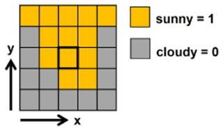
Figure 1 Demonstration for accounting for surrounding grid points. The target grid point is marked in the center. Image source: Kothe et al. (2017).

For each grid point, the number of sunny slots in the 24 pixels in the vicinity plus the center cell grid of interest is summed up (Eq. 7).

$$\begin{array}{}\text{(7)}& \mathit{\#}\text{SI}{n}_i(x,y)=\sum _{m=y-\mathrm{2}}^{m=y+\mathrm{2}}\sum _{n=x-\mathrm{2}}^{n=x+\mathrm{2}}\text{SI}{n}_i(m,n)\end{array}$$

First, for each daytime slot i, this is done. Then, to also incorporate the temporal shift in the clouds, the number of each time step is combined with the number of the previous time step for each pixel (Eq. 8).

$$\begin{array}{}\text{(8)}& \begin{array}{l}{N}_{\mathrm{1}}=\mathit{\#}\text{SI}{n}_{\mathrm{1}}\times \mathrm{0.04}\\ N_i=\left(\mathit{\#}\text{SI}{n}_i+\mathit{\#}\text{SI}{n}_{i-\mathrm{1}}\right)\times \mathrm{0.02}\end{array}\end{array}$$

The factor 0.04 is used for the first time slot of the day. For i>1, 0.02 is used. Thus, if all 25 grid points are sunny, then the resulting number N is 1 or 0 in the case that no grid point is sunny.

Thereafter, the impact of sunny and cloudy grid points on the temporal length of one time slot is estimated. The fraction of time, which slot i contributes to the daily SDU, is achieved by Eq. (9).

$$\begin{array}{}\text{(9)}& W_i=\left\{\begin{array}{lcc}max\left(N_i,C_{\mathrm{1}}\right)& \text{if}& \text{DNI}\left(C_{\mathrm{gp}}\right)\ge \mathrm{120}\mathrm{W}{\mathrm{m}}^{-\mathrm{2}}\\ N_i\cdot C_{\mathrm{2}}& \text{if}& \text{DNI}\left(C_{\mathrm{gp}}\right)<\mathrm{120}\mathrm{W}{\mathrm{m}}^{-\mathrm{2}}\end{array}\right.\end{array}$$

If the DNI in the center grid point is equal to or greater than 120 W m⁻², then the grid point is taken as sunny, and the weight (W_i) is defined by the maximum value between N_i and C₁. Otherwise, W_i is the product of N_i and C₂. These constants were derived empirically through sensitivity tests by minimizing the bias compared to reference station data in Germany. They are set as C₁=0.4, which indicates the minimum fraction that a sunny slot can contribute, and C₂=0.05, which is the weight for the contribution of a non-sunny slot (Kothe et al., 2017). The daily SDU in hours is then derived by Eq. (5).

3 Ground data and evaluation methods

To evaluate the satellite products for the period from September 2013 to December 2017, data from the INMET network were used as the ground truth. This network provides daily measurements obtained with Campbell–Stokes recorders. The stations were selected based on data availability; only stations with less than 20 % of observations missing over the study period were retained. A total of 193 stations was chosen. Quality checks were applied in order to exclude spurious data, e.g., measurements higher than its physical limits and false zeros (Gava, 2021).

Due to the considerable extension of the Brazilian territory, and the great variety of biomes and climates, the stations were grouped by climate zones, as suggested in Raichijk (2012). This classification was developed by the Brazilian Institute of Geography and Statistics (IBGE) and takes into account the average air temperature and precipitation regimes (highly anticorrelated to sunshine duration). The regions are illustrated in Fig. 2.

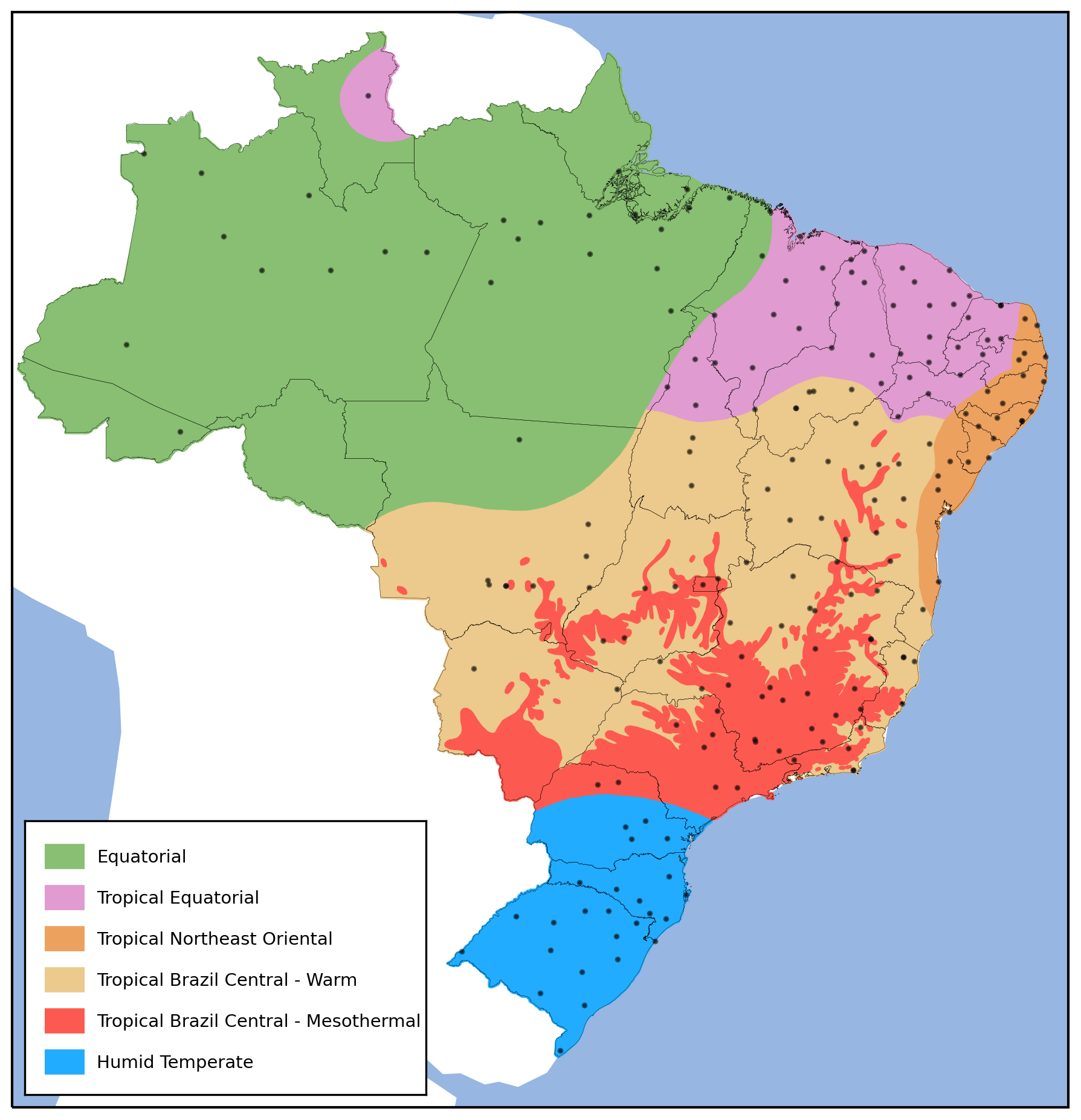
Figure 2 Spatial distribution of the INMET stations used in this study.

Figure 3 presents the box plot of SDU ground measurements for the analyzed period grouped by the climate zones. The main characteristics of the regions are described below, and the number of stations included in each one is given in parentheses.

• -

  Equatorial region (EQ; 27). This has an Af (tropical rainforest) or Am (tropical monsoon) climate, according to the Köppen–Geiger classification. It presents the average annual temperatures between 24 and 27 ^∘C and average annual precipitation of 2300 mm. It has a short dry season during austral winter, lasting under 3 months (Raichijk, 2012). The average SDU values range from 4.5 h in the wet season to 8.5 h in the dry period, which shows smaller variability. Note that for the CMSAF evaluation, 22 stations were used, since 5 of the listed stations are outside of the METEOSAT disk.

• -

  Tropical Equatorial region (TE; 43). This has an Aw (tropical savanna) or a BSh (hot semi-arid) climate, according to the Köppen–Geiger classification. It is a hot, semi-arid region, with a prolonged dry season (over 8 months). This region comprises the northeastern Brazilian Sertão, extending south until approximately 10^∘ S (Raichijk, 2012). On average, this region presents high SDU over the whole year. From June to September, the highest values are reached and the variability is low, indicating the predominance of clear-sky days.

• -

  Tropical northeast oriental region (TNO; 21). This mainly has a Aw or BSh climate, according to the Köppen–Geiger classification, with average annual temperatures ranging from 24 to 26 ^∘C. The mean SDU values are high for most of the year. Smaller SDU values are found in late austral autumn–winter. This is due to the precipitation regime of this location that exhibits the maximum precipitation rates during this period (Palharini and Vila, 2017), when it also displays the highest variability along the year.

• -

  Tropical central Brazil region. This main region was subdivided into (a) mesothermal/subwarm (hereinafter mesothermal) and (b) warm.

  • a.

    Mesothermal (TCB-M; 29). Classified as a Cw (humid subtropical) climate, this region conforms to the Köppen–Geiger classification (Raichijk, 2012). It includes part of southeastern Brazil and the area north of Paraná. This region exhibits average annual temperatures between 10 and 18 ^∘C, with dry winters. It presents great SDU variability through most of the year, with the highest mean SDU values occurring in the austral winter.

  • b.

    Warm (TCB-W; 49). This has an Aw climate, according to the Köppen–Geiger classification. This region comprises the Brazilian central plain. It is semi-humid, marked by rainy summers (December to February) and dry winters (June to August; Cavalcanti, 2009). This feature is noticeable in Fig. 3. During austral summer, the mean SDU is smaller, with higher variability.

• -

  Humid temperate region (HU; 25). It is defined as Cfa (humid subtropical climate with no dry season) by the Köppen–Geiger classification. This region presents mild temperatures between 10 and 15 ^∘C, with a well-distributed precipitation regime (without a dry season; Raichijk, 2012), which is perceptible in Fig. 3. There is no clear seasonality in the mean SDU values; moreover, there is high variability over the entire year.

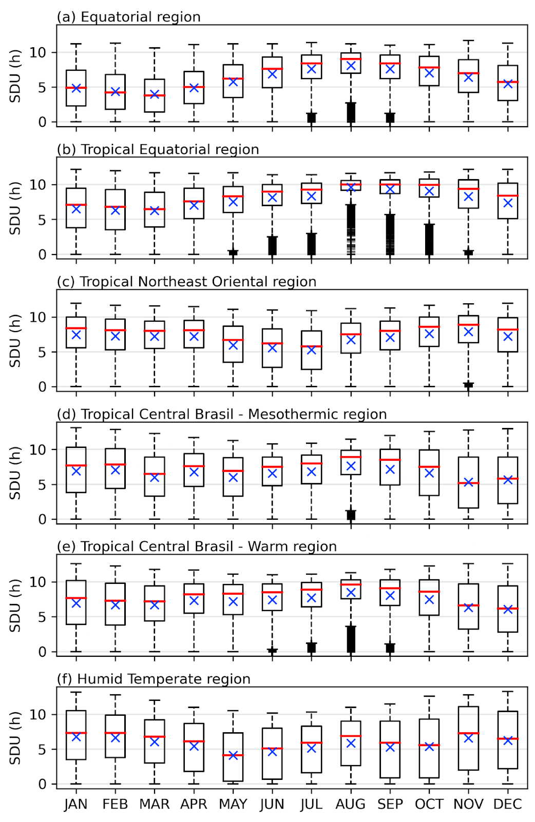
Figure 3 Box plot of SDU ground measurements. The whiskers (parallel lines extending from the boxes) indicate the variability outside of the first and third quartiles. Outliers are plotted as individual crosses. The red line indicates the median, and the blue × symbols indicate the mean.

In order to compare the satellite-based gridded SDU estimates with the in situ records, the satellite data were extracted at the station sites by selecting the satellite pixel in which the station is located. Therefore, for each month, the mean bias error (MBE), mean absolute error (MAE), root mean squared error (RMSE), and the correlation coefficient (r) of the daily SDU were calculated for every station and then grouped into the regions.

The definitions of the statistical measures are presented below (Wilks, 2011):

$$\begin{array}{c}{\displaystyle }\text{MBE}={\displaystyle \frac{\mathrm{1}}{n}}\sum _{i=\mathrm{1}}^k\left(Z_i-O_i\right)\\ {\displaystyle }\text{MAE}={\displaystyle \frac{\mathrm{1}}{n}}\sum _{i=\mathrm{1}}^k\left|Z_i-O_i\right|\\ {\displaystyle }\text{RMSE}=\sqrt{{\displaystyle \frac{\mathrm{1}}{n}}\sum _{i=\mathrm{1}}^k(Z_i-O_i{)}^{\mathrm{2}}}\\ {\displaystyle }r={\displaystyle \frac{{\sum }_{i=\mathrm{1}}^k\left(Z_i-\stackrel{\mathrm{‾}}{Z}\right)\left(O_i-\stackrel{\mathrm{‾}}{O}\right)}{\sqrt{{\sum }_{i=\mathrm{1}}^k{\left(Z_i-\stackrel{\mathrm{‾}}{Z}\right)}^{\mathrm{2}}}\sqrt{{\sum }_{i=\mathrm{1}}^k{\left(O_i-\stackrel{\mathrm{‾}}{O}\right)}^{\mathrm{2}}}}}.\end{array}$$

Thus, the variable Z describes the dataset to be validated (e.g., DISSM SDU), and O denotes the reference dataset (i.e., in situ measurements). The individual time step is marked with i, and k is the total number of time steps.

4 Results and discussion

The spatial distribution of the monthly MBE of daily SDU was generated for all months. However, Fig. 4 displays only the central months of each season, since the general behavior observed across months within seasons is very similar. It is possible to observe that the behavior of the models is homogeneous within regions. Small bias values are noticeable for the majority of the Brazilian territory for both SDU products overall, which range from −1 to 1 h. The exception is the TNO region for the CMSAF product and most of the northern and northeastern regions for the DISSM product.

Figure 4 Spatial distribution of monthly MBE (hours) between daily satellite-based SDU and in situ data for the period of 2013–2017. The DISSM (CMSAF) MBE results are shown for January, April, July, and October in panels (a), (b), (c), and (d) (e, f, g, and h), respectively. Shades of red correspond to overestimation, while shades of blue correspond to underestimation.

On the northeastern Brazilian coastline, the CMSAF method presents a significant tendency to overestimate the SDU values, exhibiting high positive MBE values and reaching 4 h in some stations.

The DISSM method presents high MBE values for the EQ, TE, and TNO regions. For the first, an overestimation tendency is observed, while the others show a negative bias. The MBE results for the TE region do not present the same homogeneity as the other zones. The eastern portion of the region shows negative values, while the states of Maranhão and Piaui do not indicate biases (values close to zero).

The MBE results over the northeastern Brazilian littoral of both products presented a marked seasonality, with smaller values during austral winter. For the DISSM method, this behavior extends to the inland of the northeastern region. This characteristic is evident in Fig. 5a. It can be seen that, from April to August, the DISSM MBE approaches zero, while the CMSAF decreases (from 1.7 h in December to 1 h). In this period, all of the summary statistics present the best results, with a smaller MAE and RMSE values (in general and under 1.5 and 2.0 h, respectively) and higher correlation coefficients (r>0.65).

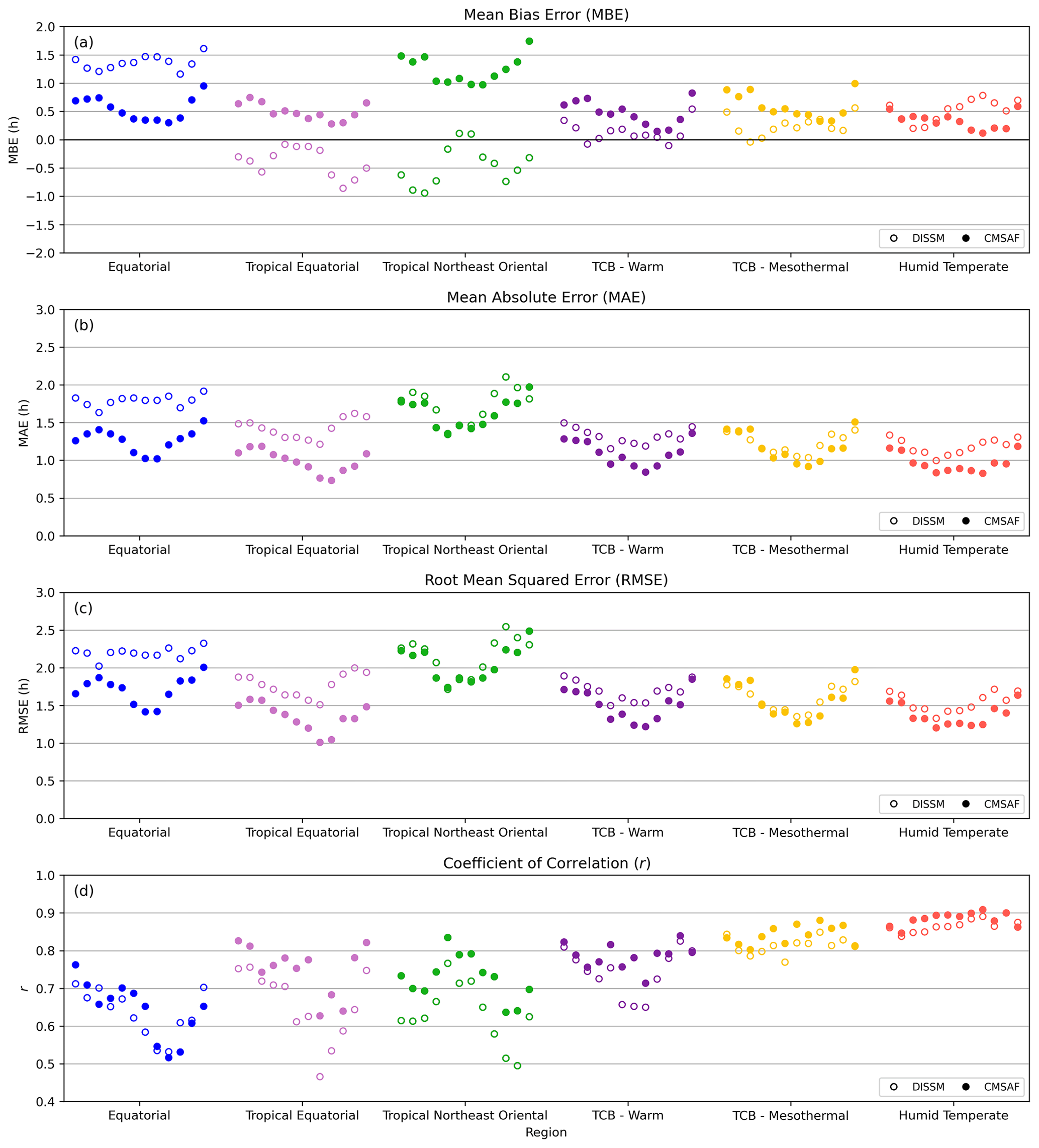
Figure 5 Summary statistics of the comparison between satellite-based SDU and ground data, on a monthly basis, over the Brazilian regions. (a) MBE, (b) MAE, (c) RMSE, and (d) r. The regions are plotted in different colors. EQ is in blue, TE is in lilac, TNO is in green, TCB-W is in purple, TCB-M is in yellow, and HU is in red. For every region, the x coordinates refer to the month of the year from January through December. Open circles (filled dots) represent DISSM (CMSAF) results.

For the other regions, the CMSAF MBE lies close to 0.5 h, with some variation, depending on the month. The DISSM method shows small biases for the southern regions, which are, on average, smaller than 0.5 h. In the EQ region, as previously mentioned, high positive biases are found, with its highest (smallest) value in December (October) at 1.61 h (1.16 h).

Figure 5b, c, and d present the MAE, RMSE, and r, respectively. Those are measurements of accuracy, and together, they can be used to acquire information regarding the data spread. Considering the MAE and RMSE, it can be noticed that the CMSAF product presents mostly smaller values than the DISSM method. Over all regions, the RMSE values are higher than the MAE, indicating the presence of outliers and some dispersion of points.

For the TE and the southern regions (TCB-W/M and HU), both products exhibit the smallest errors. The MAE (RMSE) lies, typically, under 1.5 h (2 h). These areas also present high values of r (on average, r>0.7), indicating a good agreement between the products and the in situ data, with the exception of the TE region, which presents great variability in the r results, mostly for the DISSM product.

For the EQ region, although the CMSAF MAE and RMSE results imply smaller errors compared to the DISSM data, the r results indicate the same degree of spread, which varies between 0.5 and 0.8.

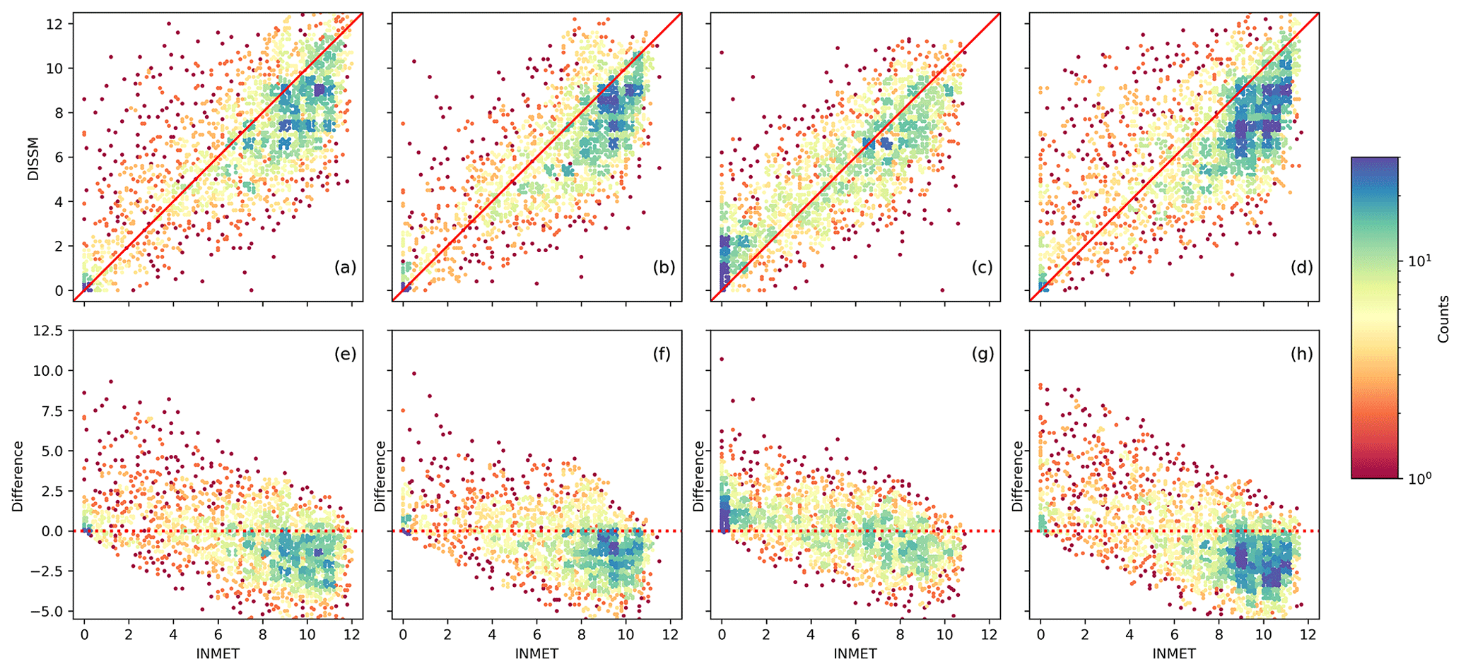
Over the TNO region, the products present high values of MAE and RMSE, with the abovementioned seasonality (smaller values during austral winter), along with highly variable values of r, which vary from 0.5 in November to 0.77 in May for the DISSM product and from 0.64 in October–November to 0.83 in May for the CMSAF method. To assess the main characteristics of the products for this region, the satellite-based data were plotted against ground measurements and for the difference between the product and observations against observations. Those scatterplots are displayed in Figs. 6 and 7 for the CMSAF and DISSM products, respectively. The data are grouped by the frequency of occurrence.

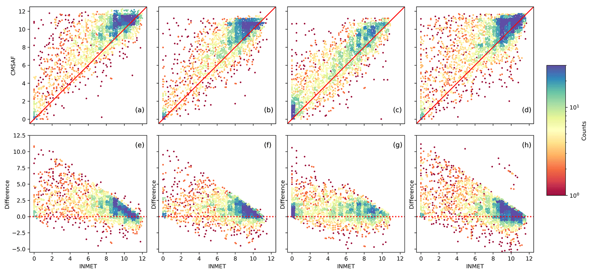
Figure 6 (a–d) Scatterplot of the CMSAF product vs. SDU in situ data for the TNO region. (e–h) Scatterplot of the difference between CMSAF product and SDU in situ data vs. SDU in situ data. Plots are grouped by frequency of occurrence. Boxes (from left to right) present the data for January, April, July, and October.

Figure 7 Same as Fig. 6 but for the DISSM product.

There is a common pattern that can be observed in both figures; an overestimation of SDU values when the ground measurements indicate 0 brightness hours. This discrepancy arises from the presence of false zeros in the SDU reference time series. On days when no data are available, SDU is assigned a value of zero, thus resulting in these false zeros. The substantial overestimation observed highlights that the steps undertaken in the quality control process were insufficient for the elimination of all erroneous data from the analysis. Despite that, it is important to note that, for non-zero values of SDU, the recorded measurements should still fall within the instrument uncertainty range of 0.1 h (Stanhill, 2003).

Figures 6a, b, and d and 7a, b, and d present a high count frequency in the upper-right corner, mainly due to the fact that, in the TNO region for the corresponding months, there is a high frequency of clear-sky days, as can be observed in Fig. 3c. So, most of the counts are concentrated above 8 h for the observed data.

In Figs. 6g and 7g, a different behavior is seen, mostly due to the higher occurrence of intermediary SDU values in this month. This is illustrated in Fig. 3c; for July, it shows that the mean SDU value is lower than that of other months and exhibits significantly higher variability. This higher variability is associated with a greater frequency of cloudiness in the region due to the rainy season. This translates into a spread of counts along the x coordinate.

In Fig. 6, it is evident that the CMSAF product tends to overestimate the SDU for all analyzed months under all-sky conditions. This is particularly clear from the scatterplots of the difference when compared to observations, as the majority of counts tend to fall above the 0.0 line. Kothe et al. (2017), when evaluating the CMSAF product, found a similar behavior on the Canary Islands (northwestern Africa), in the daily evaluation (MBE values close to 2 h), and on the west coast of Africa, in the monthly sums analysis (bias values of up to 50 h were found). The authors attributed those uncertainties to two causes, namely the frequent low-cloud fields; predominant cloud types in these regions that cause a systematic underestimation of the effective cloud albedo by the Heliosat algorithm because of the self-calibrating method (Hannak et al., 2017), thus leading to an overestimation of SDU; and to the constants used during the SDU estimates, which were derived empirically using data from Germany to take into account the contribution of different sky conditions to the SDU. Consequently, the presence of low warm clouds that are most frequent over the ocean and subtropical subsidence regions (Huang et al., 2015) may not be well represented by these parameters. This might be the case for northeastern Brazil, since low clouds with relatively warm tops are the prevailing cloud type due to subsidence in the area associated with the Walker cell (Machado et al., 2014).

In the DISSM scatterplot results, the aforementioned underestimation tendency is clearly seen, mostly under clear-sky conditions (SDU >8 h) and is less pronounced in July. In this month, it is noticeable from Fig. 7g that the counts tend to group along the zero line for low and intermediary values of SDU (SDU <8 h). For clear-sky conditions, although it still presents a tendency to underestimate the observations, the differences tend to be smaller when compared to similar values in the other months. The higher frequency of points is bounded close to −2.5 h, while in other months there is a great number of counts for differences between −2.5 and −5 h.

The better agreement between the DISSM estimates and the observations under a partly covered sky and the higher errors in clear-sky cases suggest that this might be caused by a misrepresentation of the clear-sky reflectance used in the algorithm. This characteristic was pointed out by Porfirio et al. (2020), when evaluating the global solar irradiance (a variable highly correlated to SDU; Stanhill, 2003) estimated from the GL1.2 model, and the authors also found an east–west gradient in the MBE values. They highlighted the importance of a proper assessment of the clear-sky reflectance to the estimation of the cloud cover, which is estimated in the GL1.2 in the same fashion as the SDU product.

Figure 8 presents the mean R_min fields for the central months of each season for the period from October 2013 to October 2017. This figure was constructed to help explore the R_min influence on DISSM SDU product. The fields were generated by taking the minimum (not null) reflectance values for each pixel, considering the available images in the interval between 14:00 and 16:00 UTC, within the target month. Thereafter, they were smoothed by performing 3×3 pixel means and then monthly averaged.

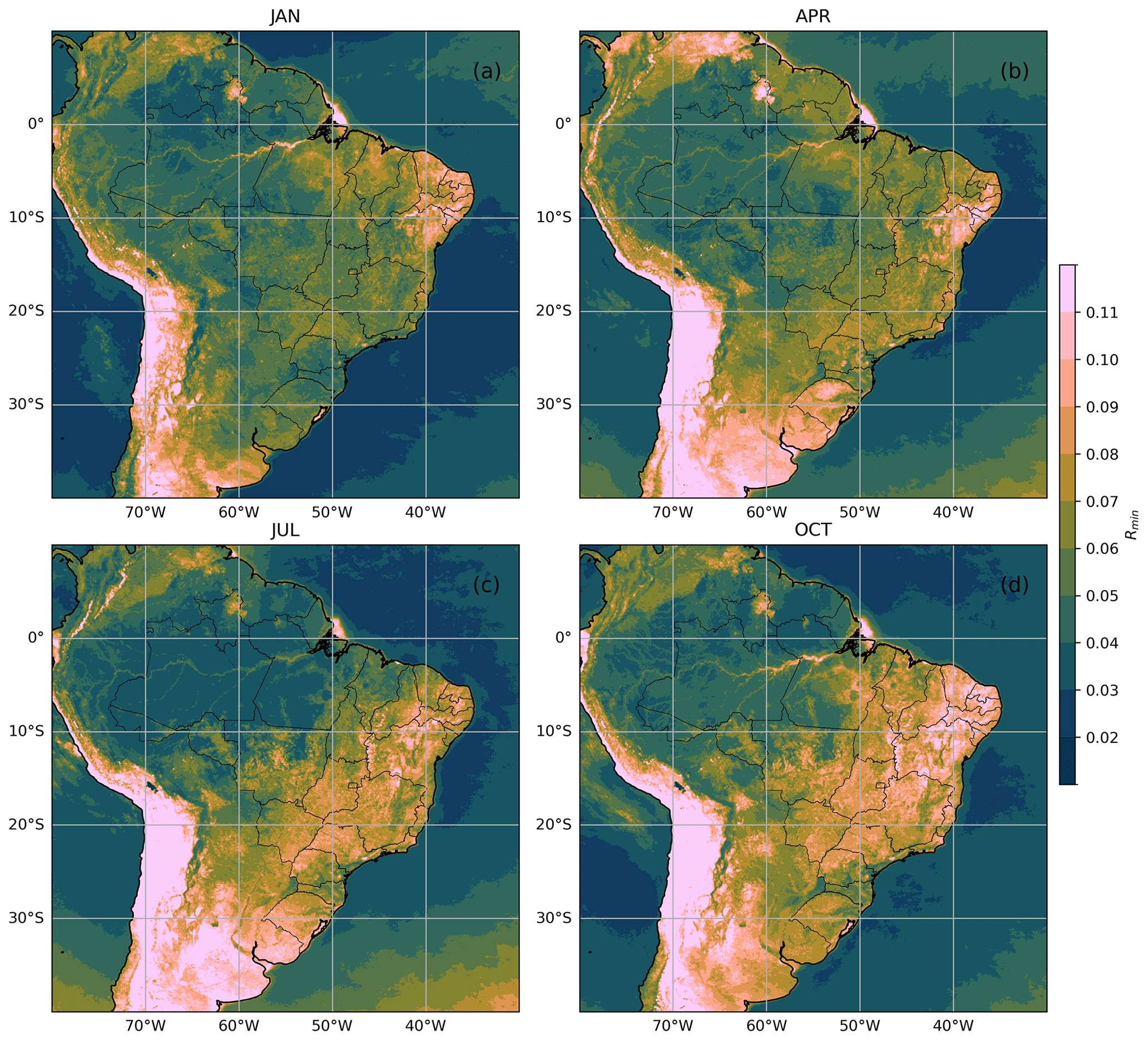
Figure 8 Average R_min obtained for each analyzed month in the period from October 2013 to October 2017. Darker (lighter) colors correspond to low (high) reflectance values.

It is noticeable that there is great variability within the country. Over Brazil, higher reflectance values are observed in northeastern Brazil and lower values in the Amazon region for all seasons, and most of the regions display seasonal variations in the clear-sky reflectance.

Evaluating the MBE results and Fig. 8, it can be seen that the R_min has a remarkable influence on the performance of the product, particularly in the northern and northeastern regions. The overestimation (underestimation) tendency found in the EQ (TNO) region seems to be related to clear-sky reflectance values being systematically lower (higher) than the R_min used in the model (0.09). This leads to an underestimation (overestimation) of cloudiness and consequently an overestimation (underestimation) of SDU. Those results suggest that the use of fields of R_min with spatiotemporal variations may improve the DISSM product results.

5 Conclusions

The agreement between two satellite-derived SDU products and in situ measurements was assessed. There are some challenges when comparing satellite-based products and station data. Satellite-derived observations are area measurements, and station records are point data; therefore, some representativeness errors are expected due to the inherently different spatial scale (Huang et al., 2016). Nevertheless, monthly bias discloses a fine agreement between SDU retrieved and observed values. Both products present low bias to most of the country (between −1 and 1 h).

Exceptions emerge for the CMSAF product on the northeastern Brazilian coastline, which reaches 4 h in some stations, and for the DISSM product on the northern portion of Brazil, where it presents a negative gradient of MBE values in the west–east direction. The best results obtained were for southern regions (TCB-W/M and HU), with MAE (RMSE) under 1.5 h (2 h) for all months and overall high values of r. In the EQ region, DISSM product presents an overestimation tendency through the year, with the highest (smallest) MBE value in December (October), 1.61 h (1.16 h). MAE and RMSE results of the CMSAF suggest lower errors when compared to the DISSM data, although the values of r indicate a similar level of variability and range from 0.5 to 0.8. CMSAF performance is remarkable, given that METEOSAT covers Brazil and particularly the EQ region with a very high satellite viewing angle, which contributes to uncertainties in the observation due to different effects. In fact, the results indicate that the algorithm is robust, and its performance seems to be independent of the viewing angle.

On the northeastern Brazilian coastline, both products exhibit a seasonal variation in performance, with a better fit for the austral winter months. However, this feature is more evident in DISSM data. During this season, both products show smaller MAE and RMSE (generally under 1.5 and 2.0 h, respectively) and higher correlation coefficients (r>0.65). For other periods, MAE (RMSE) varies between 1.5 and 2 h (2 and 2.5 h), and the CMSAF data generally have a higher correlation coefficient than the DISSM product.

In the TNO region, the systematic underestimation of the effective cloud albedo due to the low warm clouds might be the cause of the observed SDU overestimation of the CMSAF product.

The scatterplot analysis indicated that the DISSM underestimation tendency over the TNO region is more evident under clear-sky conditions (SDU >8 h), which suggests that this might be caused by a misrepresentation of the clear-sky reflectance used in the algorithm. Further investigation of the R_min showed that, in fact, in this region, the usual values of R_min are higher than the 0.09 specified in the algorithm, leading to the overestimation of the cloudiness parameter and consequently the underestimation of SDU. The opposite is observed in the EQ region, where the R_min is usually under the algorithm parameter. This suggests that including the spatiotemporal variations in R_min in the DISSM algorithm may improve its performance.

All in all, the results obtained in this study suggest that both products are adequate for providing reliable SDU data to a variety of applications. Furthermore, it is important to highlight that both products are undergoing continuous development; thus, improvements in their quality are expected. For instance, the new generation of GOES reduced the time gap between consecutive images from 30 to 10 min, and CMSAF has recently introduced an upgraded version of SARAH, which incorporates various enhancements in ancillary data, such as surface albedo, atmospheric aerosol, and water vapor profiles. These adjustments have the potential to decrease uncertainties in SDU measurements and further enhance the overall performance of these products.