Evaluation of total ozone measurements from Geostationary Environmental Monitoring Spectrometer (GEMS)

The continued interest in air pollution and stratospheric ozone variability has motivated the development of a Geostationary Environmental Monitoring Spectrometer (GEMS) for hourly ozone monitoring. This paper provides the atmospheric science community with the world's first assessment of GEMS total column ozone (TCO) retrieval performance and diurnal ozone variation. The algorithm used for GEMS is a more advanced version of its predecessor, the Total Ozone Mapping Spectrometer (TOMS) V8, that incorporates several improvements, including a new lookup table, a simple Lambertian-equivalent reflectivity model, and a spectral dependence correction. The GEMS algorithm also uses the optimal estimation method (OEM) to make error analysis more accessible and robust. The estimated retrieval errors range from 1.5 to 2 DU in September and 2 DU in December, with a constant degree of freedom of the signal (DFS) of 1 in September and a variable DFS of 1.25 to 1.4 in December throughout the day, depending on solar zenith angle (SZA). To assess the performance of the GEMS algorithm, the hourly GEMS total ozone was compared with ground-based measurements from Pandora instruments and other satellite platforms from TROPOMI (TROPOspheric Monitoring Instrument) and OMPS (Ozone Mapping and Profiler Suite Nadir Mapper). GEMS has a high correlation of 0.97 and small RMSE values compared to Pandora TCO at Busan and Seoul in South Korea. It is notable that despite exhibiting seasonal dependence in the mean bias of GEMS with Pandora, GEMS is capable of observing daily variations in ozone that are highly consistent with Pandora measurements, with a bias of approximately 1 %. The comparison of GEMS TCO data with TROPOMI and OMPS TCO data shows a high correlation of 0.99 and low RMSE compared to TROPOMI and OMPS TCO data, but the data have a negative bias of −2.38 % and −2.17 %, with standard deviations of 1.33 % and 1.57 %, respectively. Similar to OMPS, the influence of SO₂ from volcanic eruptions is not properly removed in some regions, leading to GEMS overestimating TCO in those areas. The mean biases of GEMS TCO data with TROPOMI and OMPS TCO are within ±1 % at low latitudes but become negative at midlatitudes, with an increasingly negative dependence on latitude. Furthermore, this dependence becomes more prominent from summer to winter. The empirical correction applied to the GEMS irradiance data improves the dependence of the mean bias on season and latitude, but a consistent bias still remains, and a marginal positive trend was observed in December. Therefore, further investigation into correction methods is needed. The results are a meaningful scientific advance by providing the first validated, hourly UV ozone retrievals from a satellite in geostationary orbit. This experience can be used to advance research with future geostationary environmental satellite missions, including the incoming TEMPO (Tropospheric Emissions: Monitoring of Pollution) and Sentinel-4.

1 Introduction

Stratospheric ozone is responsible for absorbing the Sun's ultraviolet (UV) radiation, protecting the Earth's surface from harmful UV rays. Ozone in the troposphere is a toxic air pollutant that affects human health via harmful respiratory and cardiovascular effects and negatively affects vegetation growth (Crutzen, 1979; Jacob et al., 1999). Global ozone monitoring is therefore essential for both public health and environmental protection to provide valuable information about the state of the atmosphere and identify areas where public action is needed to reduce the impacts on human health and the environment (Engel et al., 2019; WMO, 2014).

Satellite remote sensing is a powerful tool for monitoring atmospheric ozone with high spatial and temporal coverage of global observations (Fishman et al., 2008; Fishman and Larsen, 1987). Global ozone monitoring by the Total Ozone Monitoring Spectrometer (TOMS) aboard the Nimbus-7 satellite in 1978 was the first mission dedicated to creating detailed maps of atmospheric ozone from space (Bhartia et al., 1996). Since then, the Global Ozone Monitoring Experiment (GOME; Burrows et al., 1999), SCanning Imaging Absorption spectroMeter for Atmospheric CHartographY (SCIAMACHY; Bovensmann et al., 1999), Ozone Monitoring Instrument (OMI; Levelt et al., 2006), Ozone Mapping and Profiler Suite Nadir Mapper (OMPS; Flynn et al., 2014), and TROPOspheric Monitoring Instrument (TROPOMI; Veefkind et al., 2012), which all built on the success of TOMS, have provided a continuous and consistent mapping of atmospheric ozone.

The continued interest in air pollution and stratospheric ozone variability has motivated the development of new satellite missions with improved capabilities for hourly monitoring of atmospheric composition. The Geostationary Air Quality (Geo-AQ) constellation missions such as the Geostationary Environmental Monitoring Spectrometer (GEMS), Sentinel-4, and Tropospheric Emissions: Monitoring of Pollution (TEMPO) were designed to provide high-quality measurements of atmospheric composition throughout the day from a geostationary orbit (Ingmann et al., 2012; Zoogman et al., 2017; Kim et al., 2020). These new missions will provide more accurate and timely information about air quality and stratospheric ozone for supporting air quality forecasts and policy-making. The GEO-Kompsat 2B satellite carrying the GEMS sensor was the first mission of the Geo-AQ constellation, which was launched on 18 February 2020 (Kim et al., 2020). GEMS is a UV-visible spectrometer that measures direct solar irradiance and radiance backscattered from the Earth's surface and atmosphere covering the Asia–Pacific region (Kim et al., 2020).

Since GEMS is the first Geo-AQ mission, it is necessary to introduce the algorithm process and new data products to provide information for users. Here we focus on the GEMS total ozone (O3T) algorithm for retrieving the total column ozone (TCO) from GEMS level 1B (L1B) radiance spectra and the validation of these data using ground-based Pandora TCO measurements and other satellite TCO measurements from OMPS and TROPOMI. The GEMS O3T algorithm has several improvements over previous algorithms, such as the use of a new lookup table (LUT), a simple Lambertian-equivalent reflectivity (LER) model and the correction for spectral dependence of LER, and the use of GEMS level 2 (L2) cloud product. The algorithm is now flexible enough to handle additional wavelengths and more readily employ different sources of a priori profile information without significant changes to the design of the algorithm. The GEMS O3T algorithm also uses the optimal estimation method (OEM) to make error analysis more accessible and robust.

This paper consists of five sections. Section 2 describes the GEMS instrument and level 1B data. Section 3 explains the differences and advantages of the GEMS algorithm from its predecessor, the TOMS algorithm. Section 4 discusses the results of the retrieval characteristics and error analysis. Section 5 presents the validation results of the new TCO product with respect to ground-based Pandora TCO measurements and other satellite TCO measurements from OMPS and TROPOMI. Section 6 discusses the impact of the new algorithm on global TCO observations and is followed by a conclusion in Sect. 7.

2 Data and method

2.1 The GEMS mission

GEMS is a UV-visible spectrometer developed for South Korea's next-generation geostationary multipurpose satellite program, which consists of two satellites, GEO-KOMPSAT 2A (GK-2A) and GEO-KOMPSAT 2B (GK-2B). They are colocated at 128.2^∘ E over the Equator. The GK-2A satellite is equipped with an Advanced Meteorological Imager (AMI) to provide high-resolution images of the Earth's surface and atmosphere for weather forecasting, while GK-2B has two payloads, namely one with the GEMS sensor to monitor the atmospheric composition and air quality and another with a Geostationary Ocean Color Imager (GOCI)-II to monitor the ocean color.

GEMS is designed to use the same optical path for direct solar radiation and radiance backscattered from the Earth's surface and atmosphere. Using the same optical path for solar irradiance and radiance backscattered from Earth has several benefits. First, it minimizes calibration uncertainty in algorithms using the ratio of radiance to solar irradiance because sensor errors common to the radiance and irradiance measurements cancel. The measured light passes through the same calibration assembly and scan mirror, telescope, spectrometer, and detectors, which minimizes the possibility of inconsistency between the measurements. However, a diffuser is used for solar irradiance measurements and is located in front of the scan mirror and introduces a source of calibration error that does not cancel in the radiance : irradiance ratio. The magnitude of this error is difficult to quantify and requires both in-flight calibration measurements and theoretical calculations. We will discuss the impact of this error in the retrieval and how to correct it in Sect. 4.

GEMS measures Earth radiance in the 300–500 nm wavelength range, with a high spectral sampling of 0.2 nm and spectral resolution of 0.6 nm. The spatial resolution of the instrument is 3.5 km × 7 km over Seoul, South Korea, and the overall field of regard (FOR) is from 45^∘ N to 5^∘ S latitude and between 75^∘ E and 145^∘ E longitude for every hour from 09:00 to 17:00 Korea standard time (KST). Solar irradiance is measured over the same wavelength range once per day in the nighttime darkness. The incident light from the telescope is dispersed onto a single two-dimensional charge-coupled device (CCD), which has 1033 spectral pixels and 2048 pixels in the spatial dimension. A two-axis mirror scans from east to west with a fixed north–south field of view during 30 min observation periods, which collect measurements across the entire FOR.

2.2 The GEMS algorithm

A major objective of this study was to obtain total ozone data from the geostationary orbit for the first time using the UV spectrum. The GEMS O3T algorithm was developed based on the well-researched NASA TOMS algorithm, which is the oldest and most proven method of satellite total ozone retrieval algorithms developed by Dave and Mateer (1967). Since several others have documented earlier versions of the TOMS algorithm over a half-century of development (Bhartia and Haffner, 2012; Bhartia, 2002; Dave and Mateer, 1967; Haffner et al., 2015; Klenk et al., 1982; McPeters et al., 1996), the important goal of using the TOMS algorithm for GEMS is to obtain the most stable and reliable total ozone output. Because the TOMS algorithm was only applied to total ozone retrievals from a sun-synchronous orbiting satellite, we conducted a series of studies to improve the total ozone data quality with the GEMS O3T algorithm. The flowchart represents the total ozone retrieval process from the improved GEMS O3T algorithm in Fig. 1. The algorithm consists of two main components, namely a forward model that calculates the top-of-atmosphere (TOA) radiance and an inverse model that derives total ozone from the measured radiance.

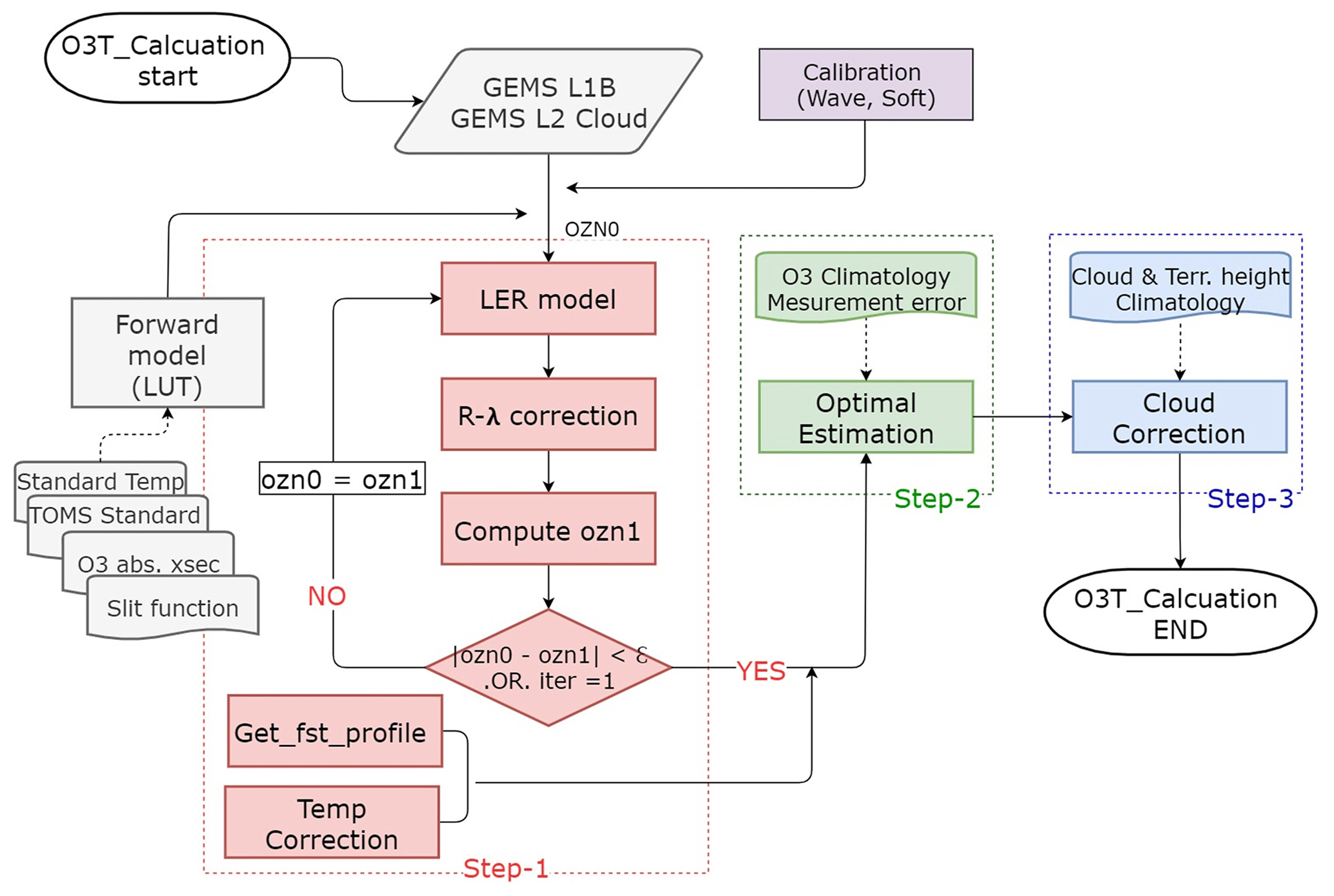
Figure 1 Flowchart of GEMS O3T retrieval algorithm, consisting of a forward model for TOA radiance calculation and an inverse model for total ozone derivation. Steps 1–3 are highlighted with pink, green, and blue, respectively.

2.2.1 Forward model

The TOA radiance at the seven wavelengths (312.34, 317.35, 331.06, 340, 354, 360, and 380 nm) is calculated by the VLIDORT radiative transfer model (RTM; Spurr, 2008). We used a precalculated radiance lookup table, since performing the VLIDORT calculations online is time-consuming for an operational algorithm. The precalculated radiances are obtained at different solar zenith angles, satellite viewing angles, and reflecting surface conditions (land and ocean, clouds, and aerosols) for TOMS standard ozone profiles that vary with latitude band and total ozone amount (Bhartia, 2002; Wellemeyer et al., 1997). Due to the limited observational range of GEMS, which covers only low- and midlatitude regions, we employed a reduced set of 11 ozone profiles out of the 21 TOMS standard profiles in our radiance calculations. The surface underlying the atmosphere is assumed to have the Lambertian-equivalent reflectivity (LER) which treats surfaces, clouds, and aerosols as Lambertian reflectors at terrain pressure (Ahmad, 2004). Our VLIDORT radiance calculations consider polarized Rayleigh scattering and the O₃ absorption, with temperature-dependent gaseous absorption cross sections. This study used the Brion–Daumont–Malicet (BDM) ozone absorption cross section (Daumont et al., 1992; Brion et al., 1993; Malicet et al., 1995). VLIDORT is also used when calculating the lookup tables (LUTs) for Jacobians, which are needed to perform the retrieval using optimal estimation. We used a single USA standard temperature profile to optimize the table size for radiances and Jacobians. Calculated radiances are then adjusted using a zonal mean temperature climatology via a temperature correction in the algorithm. Supplementary sections provide an elaborate account of the radiance LUTs used in the GEMS O3T algorithm and an evaluation of the errors that arise during LUTs interpolation.

2.2.2 Inverse model

An inverse model in the GEMS O3T algorithm is a mathematical tool that helps to convert the measured radiance into geophysical parameters, such as the total ozone and ozone profile. The model proceeds in three steps. Details of the individual steps are presented below. In step 1, the reflectivity is derived at 380 nm, then corrected by the method suggested by Dave (1978), followed by the first-guess estimate of ozone with 317.35 nm, and finally, residuals and Jacobians are calculated. Step 2 is a straightforward implementation of an optimal estimation method to estimate the ozone profiles using inputs derived in step 1 and a set of radiances (312.34, 317.35, and 331.06 nm) and a priori ozone profiles and their error covariance matrix. This process, which is not present in the TOMS V8 algorithm, is the core of the GEMS O3T algorithm because it provides the error amount for retrieved total ozone and the degree of freedom that shows the independent vertical information of the ozone profile. The correction for clouds and terrain height is made in the final process of step 3.

Step 1 process starts with the computation of reflectivity using the measured backscatter ultraviolet (BUV) radiance at 380 nm, based on the simple Lambertian-equivalent reflectivity (SLER) model. The initial assumptions are that the spectral dependence of reflectivity (R) is zero (i.e., $\mathrm{d}\mathit{R}/\mathrm{d}\mathit{\lambda }=\mathrm{0}$). However, this assumption can no longer be valid in the presence of absorbing aerosol, sea glint, and clouds ($\mathrm{d}\mathit{R}/\mathrm{d}\mathit{\lambda }\ne \mathrm{0}$). The algorithm accounts for radiative effects of aerosols and surface reflectance by using the calculated spectral slope of $\mathrm{d}\mathit{R}/\mathrm{d}\mathit{\lambda }$ obtained from reflectivity at 340 and 380 nm, with negligible ozone absorption cross sections in Eq. (1).

$$\begin{array}{}\text{(1)}& \mathit{R}={\mathit{R}}_{\mathrm{380}}+{\displaystyle \frac{\mathrm{d}\mathit{R}}{\mathrm{d}\mathit{\lambda }}}\left({\mathit{\lambda }}_{\mathrm{317}}-{\mathit{\lambda }}_{\mathrm{380}}\right)\end{array}$$

This calculation updates the estimated reflectivity (R) derived after each iteration proposed by Dave (1978). However, in the presence of high amounts of UV-absorbing aerosols, $\mathrm{d}\mathit{R}/\mathrm{d}\mathit{\lambda }$ cannot be linear and results in a significant error in the derived reflectivity. These data are flagged during the quality control process. The dependence of the backscattered radiance on ozone is approximately exponential. A quantity called the N value is defined to reduce the dynamic range of the total ozone dependence (Klenk et al., 1982). The N value is defined as follows:

$$\begin{array}{}\text{(2)}& N=-\mathrm{100}{\log }_{\mathrm{10}}{\displaystyle \frac{I}{F}},\end{array}$$

where F is the extraterrestrial solar irradiance. The amount of total ozone is determined when the measured N value (N_m) at 317.35 nm is equal to the calculated one (N_c), with the total ozone amount corresponding to the TOMS standard ozone profile at a given satellite viewing geometry, solar zenith angle, surface reflectivity, and surface pressure (Bhartia, 2002). The interpolation entails using three to eight ozone profiles, each with a different range of total ozone amounts for latitude. Therefore, the ozone profile shape corresponding to the retrieved total ozone is obtained by this process.

The OEM approach proposed by Rodgers (2000) is applied in step 2 to retrieve a coarse ozone profile, which is estimated from a set of radiances at three wavelengths with different amounts of ozone absorption (312.34, 317.35, and 331.06 nm) using a priori profiles and their error covariance matrices. The use of an optimal estimation allows a smooth transition between the use of the different wavelengths, and thereby eliminates the discontinuities associated with TOMS ozone distribution that occurs when the solar angle is large.

$$\begin{array}{}\text{(3)}& \begin{array}{rl}\widehat{x}& =x_{\mathrm{a}}+{\mathbf{S}}_{\mathrm{a}}{\mathbf{K}}^{\mathrm{T}}{\left({\mathbf{KS}}_{\mathrm{a}}{\mathbf{K}}^{\mathrm{T}}+{\mathbf{S}}_{\mathrm{e}}\right)}^{-\mathrm{1}}\\ & [\left({\mathit{N}}_{\mathrm{m}}-{\mathit{N}}_{\mathrm{1}}\right)+\mathbf{K}\left(x_{\mathrm{1}}-x_{\mathrm{a}}\right)];\\ \mathbf{G}& ={\mathbf{S}}_{\mathrm{a}}{\mathbf{K}}^{\mathrm{T}}{\left({\mathbf{KS}}_{\mathrm{a}}{\mathbf{K}}^{\mathrm{T}}+{\mathbf{S}}_{\mathrm{e}}\right)}^{-\mathrm{1}};\\ \mathbf{A}& =\mathbf{GK};\\ \widehat{\mathbf{S}}& ={\mathbf{S}}_{\mathrm{a}}-{\mathbf{S}}_{\mathrm{a}}{\mathbf{K}}^{\mathrm{T}}{\left({\mathbf{KS}}_{\mathrm{a}}{\mathbf{K}}^{\mathrm{T}}+{\mathbf{S}}_{\mathrm{e}}\right)}^{-\mathrm{1}}{\mathbf{KS}}_{\mathrm{a}},\end{array}\end{array}$$

where $\widehat{x}$ is the optimized ozone profile consisting of 11 Umkehr layers. The pressure at the bottom of these layers decreases by a factor of 2, starting from the mean sea level pressure (1013.25 hPa) to 0.99 hPa. The top layer goes from all altitudes above the 0.99 pressure level. x_l is the ozone profile retrieved in step 1. The x_a is the a priori ozone profile obtained from McPeters–Labow (ML) climatological profiles (McPeters and Labow, 2012), consisting of 12 months and 18 latitudinal bands with 10^∘ intervals from 90^∘ N to 90^∘ S. The S_a is a priori error covariance matrix (11×11 covariance matrix) derived from the ML climatological profile, where the correlation is limited to one layer from the diagonal entry. N_m is the measurement radiance vector consisting of three elements from 312, 317, and 331 nm, and N₁ is the N value calculated from x₁. S_e is the measurement error covariance matrix and is assumed to be a diagonal matrix where the elements are the squares of the assumed measurement errors. We assume a measurement error of 0.12 %, according to GEMS signal-to-noise ratio (SNR) corresponding to 320 nm. K is the Jacobian matrix, defined as $\mathrm{d}{N}_j/\mathrm{d}{x}_i$ for each layer i and wavelength j, representing the partial derivatives of the forward model to the ozone. The gain matrix, G, measures how sensitive the retrieved profile is to measurement errors, and the averaging kernel matrix, A, provides the sensitivity of the retrieval to a change in true ozone profile and a vertical resolution of the retrieved profile. The covariance matrix $\widehat{\mathbf{S}}$ measures the degree of error in the retrieved ozone profile. It contains the measurement and smoothing errors propagated through the G and A matrices, respectively. The optimal estimation technique also offers crucial parameters for error analysis, including the degrees of freedom for signal (DFS), retrieved column estimated error, and column-weighting functions (CWFs). The Supplement provides a comprehensive elucidation of these variables.

The total ozone obtained from step 2 assumes that the reflecting surface is at sea level. If the surface is at a different elevation or a cloud is present, then we must account for it in the total ozone calculation. After adjusting the CWFs (w_l) for the profile used, the final step 3 total ozone is calculated by subtracting the amount of ozone corresponding to the difference between the topography (or cloud) height and the ground surface from the step 2 total ozone. Since the ozone column below the cloud pressure (p_c) is relatively small, we use a relatively simple method to correct it. If reflectivity (R) from 380 nm is less than 0.05 (R_s) or snow or ice is present, then no cloud is assumed. If R is greater than 0.4 (R_c), then we assume the entire pixel is covered with clouds. For $R_{\mathrm{s}}<\mathit{R}<R_{\mathrm{c}}$, the pixel was assumed to be partial cloud cover, and the cloud fraction was determined by Eq. (4) as follows:

$$\begin{array}{}\text{(4)}& f_{\mathrm{c}}=\left(\mathit{R}-R_{\mathrm{s}}\right)/\left(R_{\mathrm{c}}-R_{\mathrm{s}}\right).\end{array}$$

We assume that this fraction (f_c) is approximately the fraction of the measured radiance signal reflected by clouds within the instrument field of view. We first estimate the ozone between the cloud and terrain pressure in each layer l and then set the (w_l) in layers below p_c to zero in Eq. (5).

$$\begin{array}{}\text{(5)}& \begin{array}{l}{x}_l^{\ast }=\widehat{x_l}\left(\mathrm{1}-f_{\mathrm{c}}\right)+x_{\mathrm{a},l}{f}_{\mathrm{c}},\\ w_l^{\mathrm{c}}={\mathit{w}}_l\left(\mathrm{1}-f_{\mathrm{c}}\right),\end{array}\end{array}$$

where $\widehat{x_l}$ and x_a,l are the ozone amount in layer l of the profile obtained from step 2 and from the a priori profile respectively. Then, the correction to the total column is obtained by

$$\begin{array}{}\text{(6)}& \mathit{\delta }\mathrm{\Omega }={\sum }_{l=\mathrm{0}}^{l_{\mathrm{pc}}}{x}_l^{\ast }\left(\mathrm{1}-w_l^{\mathrm{c}}\right)-\widehat{x_l}\left(\mathrm{1}-w_l^{\mathrm{c}}\right).\end{array}$$

2.3 Correlative satellite measurements

OMPS was launched in October 2011 on the Suomi National Polar-orbiting Partnership (SNPP) satellite and includes both nadir- and limb-viewing modules. OMPS Nadir-Mapper (NM) total ozone data (OMPS NMTO3) were used in this study. The OMPS NM is a hyperspectral imaging push-broom sensor, with a 110^∘ cross-track field of view (FOV) and 35 cross-track positions. OMPS NM has a 50 km × 50 km spatial resolution at the nadir and measures solar backscattered ultraviolet radiation in the spectral range from 300 to 380 nm. The OMPS total ozone algorithm is based on the NASA Version 8 total ozone algorithm (Bhartia, 2002). In our study, operational OMPS NM Level 2 (L2) version 2.1 data were used. As validated in McPeters et al. (2019), the maturity of this product is high, with biases smaller than 0.2 % when compared to ground-based measurements in the Northern Hemisphere.

TROPOMI was launched in October 2017 on the Sentinel-5 Precursor (S5P) satellite. TROPOMI aboard S5P is a nadir-viewing spectrometer that provides measurements in the ultraviolet, visible, near-infrared, and shortwave infrared spectral bands. TROPOMI has a swath width of 2600 km (roughly 104^∘ wide), with a ground pixel resolution of 3.5 km × 5.5 km (Veefkind et al., 2012). S5P–TROPOMI offline (OFFL) total ozone column products were used in this study which are obtained using the GODFIT (GOME Direct Fitting approach) version 4 retrieval (Lerot et al., 2021; Spurr et al., 2021). The algorithm directly compares with simulated radiances through nonlinear least-squares inversion, using the sun-normalized measured radiance from 325 to 335 nm. The calculated radiances and Jacobians are obtained with the RTM LIDORT (LInearized Discrete Ordinate Radiative Transfer; Spurr, 2008). A validation for S5P–TROPOMI OFFL TCO with global ground-based measurements from April to November 2018 was found to be well within the acceptable limits, with mean biases (MB) ranging from 0 % to 1.5 % and standard deviations (SDs) between 2.5 % and 4.5 % for monthly mean co-locations (Garane et al., 2019).

2.4 Correlative ground-based measurements

The Pandora TCO retrieval algorithm utilizes a modified version of the differential optical absorption spectroscopy (DOAS) technique to determine the concentration of atmospheric constituents. In the case of TCO, the DOAS method compares the direct solar spectra measured by the Pandora spectrometer to an independent extraterrestrial reference spectrum, which represents the expected solar spectrum in the absence of atmospheric absorption. Through spectral analysis of the measured and reference spectra within the 305 to 328.6 nm wavelength range, the Pandora algorithm retrieves TCO values using a spectral fitting approach, wherein fitting parameters are optimized to minimize the difference between the measured and modeled spectra. Additionally, the Pandora algorithm accounts for the effects of Rayleigh scattering and atmospheric absorption species such as NO₂ and O₄. Technical details about the retrieval algorithm and configuration settings are available in the software manual (Cede et al., 2021). The TCO used in this study was processed and retrieved by using the Blick Software Suite (version 1.7).

3 Results and discussion

3.1 GEMS hourly total ozone distribution

The GEMS sensor on board a geostationary satellite has the advantage of measuring ozone over current low Earth orbit (LEO) satellite sensors because it provides hourly observations throughout the data, which helps to improve our understanding of ozone. GEMS V2.0 total ozone products are used in our analysis. To assess the performance of the GEMS total ozone algorithm, the hourly GEMS total ozone on 29 March 2021 is shown in Fig. 2. This figure shows the 8 h GEMS total ozone measurements from 09:00 to 16:00 KST. Because GEMS measures backscattered UV radiation when the solar zenith angle is not large, the daytime hourly observation time and area vary, depending on the season (NIER, 2020a). Figure 2a shows the hemisphere east (HE) mode at 09:00 KST, Fig. 2b shows the hemisphere Korea (HK) mode at 10:00–11:00 KST, Fig. 3c–d show the full central (FC) mode at 11:00–12:00 KST, and Fig. 2e–h show the full west (FW) mode at 13:00–16:00 KST. The GEMS observation usually takes 30 min and runs from 15 min before the hour to 15 min after the hour.

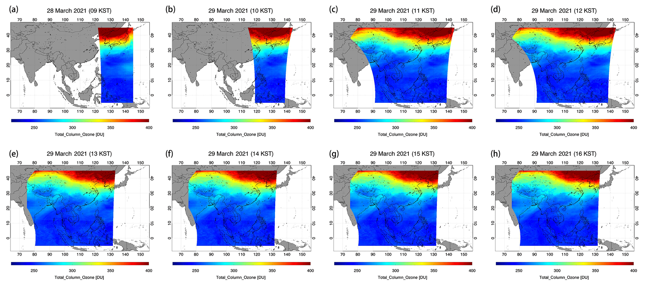
Figure 2 Hourly GEMS total ozone distribution on 29 March 2021.

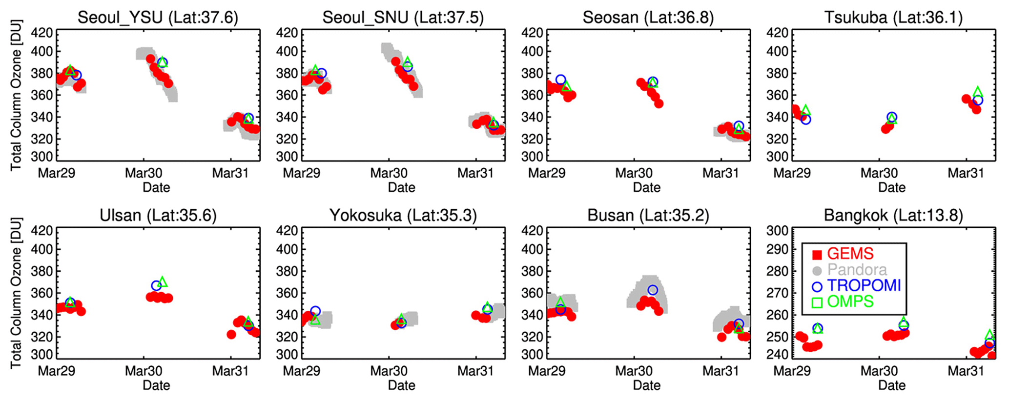
Figure 3 Comparison of GEMS TCO with Pandora, TROPOMI, and OMPS TCO from 29 to 31 March 2021 over eight Pandora sites. The TCO measurements are represented with red-filled squares for GEMS, gray-filled circles for Pandora, blue circles for TROPOMI, and green squares for OMPS.

The total ozone distribution, ranging from 250 to 400 DU, shows a typical distribution in March, with high values at high latitudes, followed by a sharp decrease in the midlatitudes and gradually decreasing toward the Equator. Because the scale bar is so large, changes in hourly values are not clearly seen. The GEMS hourly ozone monitoring system provides continuous updates on stratospheric ozone and its associated atmospheric changes. It also provides essential information to models that help us predict the future development in the ozone state.

Figure 3 compares the hourly GEMS TCO with Pandora TCO observed over eight ground sites and satellite TCO for 3 consecutive days from 29 to 31 March 2021. The hourly total ozone distribution in Fig. 3 showed significant diurnal ozone changes of up to 40 DU. This indicates that the ozone undergoes significant diurnal change, primarily due to changes in stratospheric ozone, and this is evidence of why hourly ozone monitoring is important to track dynamic ozone changes. Pandora TCO varies considerably over time, and the diurnal variation in the GEMS is in good agreement with that of Pandora. The GEMS data for diurnal ozone change offer advantages over TROPOMI (blue) and OMPS (green) ozone data, which are observed once per day.

3.2 Validation of GEMS total ozone measurements with Pandora

Satellite measurements are subject to instrument measurement errors and retrieval errors from ill-posed problems. Therefore, validation is essential for scrutinizing satellite retrieval accuracy and providing confidence in the final results. The GEMS total ozone data were validated by comparing them with ground-based Pandora and other satellite measurements from OMPS and TROPOMI. For accurate validation, we used GEMS TCO between August and December 2020, a stable initial operation period with accurate image navigation and registration (INR) information. The available Pandora observations during this period were over Busan, Ulsan, Seoul, and Yokosuka. Table 1 presents detailed Pandora site information. Since GEMS switches to full west mode at 13:00 KST in November and December, there is no GEMS measurement at Yokosuka in Japan from this time, so we used only data before this time for validation. GEMS takes 30 min to complete an observation over the FOR, whereas Pandora collects each measurement in 2 min several times per day. For temporal coincidence, we used the average of Pandora observation data before and after 15 min of the local GEMS observation. For spatial coincidence, we used the closest GEMS data to the Pandora site. To exclude Pandora data contaminated by clouds and aerosols, we used data with the normalized root mean square (rms) of the weighted spectral fitting residuals less with than 0.05 % and the estimated error in TCO of less than 2 DU, as suggested by Tzortziou et al. (2012). We take GEMS data with a solar zenith angle of smaller than 75^∘ to avoid GEMS errors that may occur due to the high solar zenith angle of GEMS data.

Table 1 Pandora observation sites over the GEMS comparison domain.

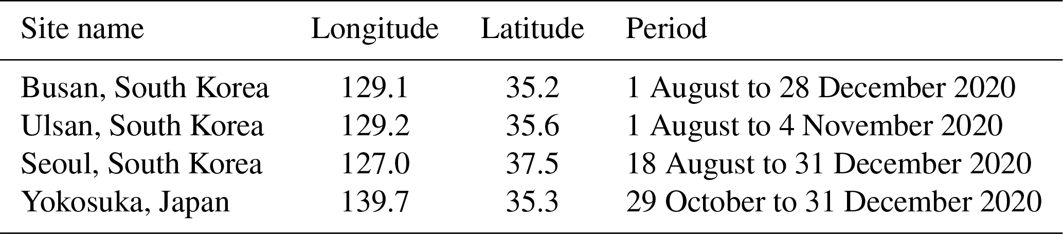
Figure 4 represents the comparison of GEMS, TROPOMI, and OMPS with Pandora TCO at the sites. The comparison between GEMS and Pandora was performed at 03:45 and 04:45 UTC, which correspond to the overpass time of TROPOMI–OMPS, in order to exclude potential errors that vary throughout the day and were not taken into account in this comparison. Figure 4a shows a high correlation of 0.97 or more with GEMS and Pandora TCO at Seoul and Busan but a low correlation of 0.90 at Ulsan, which is significantly smaller than at other sites. RMSE showed satisfactory small values, with the lowest RMSE of 1.3 DU. As mentioned earlier, because GEMS operates in full west mode, starting at 13:00 KST during November and December, and there are no GEMS measurements at the overpass time of TROPOMI–OMPS in Yokosuka, Japan. Mean biases (MBs) ranging from −1.36 % to 0.76 % were observed at all sites, with the highest positive MBs occurring in August. The MBs showed a distinctly high value in August (summer), with 3.30 % in Busan and 2.87 % in Seoul, which then decreased to 0.54 % and −1.36 % in December (winter), respectively. Overall, it is noteworthy that the mean biases (MBs) of GEMS–Pandora decrease significantly over time, decreasing from August to October before slightly increasing in December.

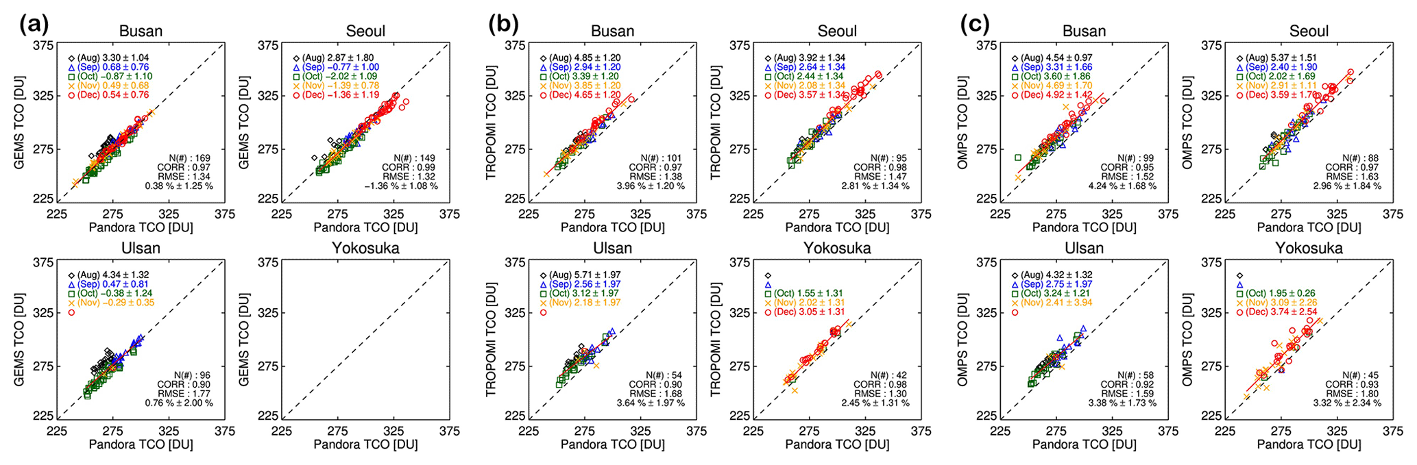
Figure 4 Scatterplots of Pandora TCO with (a) GEMS TCO, (b) TROPOMI TCO, and (c) OMPS TCO at Busan, Seoul, Ulsan, and Yokosuka. A linear fit representing a 1:1 ratio is shown in dotted black lines. The legends of N, CORR, RMSE, and the number in percentage represent the number of data points, correlation coefficient, RMSE, and mean bias with standard deviation (SD), respectively. The number on the bottom right is the percentage bias for each month. The comparison between GEMS and Pandora was conducted at the overpass time of TROPOMI–OMPS to eliminate potential errors that vary over the course of the day and were not included in this comparison. As mentioned earlier, this is because GEMS operates in full west mode starting at 13:00 KST during November and December, and there are no GEMS measurements at the overpass time of TROPOMI–OMPS in Yokosuka, Japan.

Figure 4b and c show the comparison of Pandora with other satellite data, TROPOMI, and OMPS. Their correlation is similar to that of GEMS and Pandora. The correlation of Pandora with OMPS and TROPOMI is the lowest in Ulsan, at 0.92 and 0.90, respectively. There seems to be an issue with the Pandora measurements at Ulsan. The RMSE between Pandora and both satellites was less than 2 DU, as in GEMS.

Although no monthly trend was observed as distinct as GEMS, the MB in TROPOMI and OMPS increased in August (summer) and December (winter). The reason for this is that, as Herman et al. (2015) showed, the satellite retrieval methods perform a temperature correction for the temperature-sensitive ozone absorption coefficient, whereas Pandora uses a fixed-temperature ozone absorption coefficient. Therefore, comparisons of satellite and Pandora data may show seasonal dependence. However, the seasonal variability shown in the comparison of GEMS and Pandora differs from those between TROPOMI (OMPS) and Pandora in magnitude and seasonal dependence.

Figure 5 is a time series showing the percentage difference between three satellite observations (GEMS, TROPOMI, and OMPS) and Pandora. The overall mean bias for TROPOMI–Pandora and OMPS–Pandora is within 3.8 % for all stations, which is consistent with the previous studies (Herman et al., 2015). As for the mean standard deviation, TROPOMI has lower variability in comparison to OMPS. This could be due to the lower spatial resolution of OMPS at 50 km × 50 km when compared to TROPOMI at 5.5 km × 3.5 km. In the case of Ulsan, both comparisons of TROPOMI and OMPS with Pandora showed a low correlation (∼0.90) and a high standard deviation (∼1.8 %) when compared to other stations. These comparison results suggest that the Pandora measurement at Ulsan suffers from problems in the accuracy of total ozone measurement, which may be due to some form of instrument error. Therefore, we have excluded the Pandora measurements at Ulsan from a reference data set for further GEMS validation at this time. The mean bias of GEMS with Pandora is 0.11 %, with a standard deviation of 2.17 % for all stations. The comparison with Pandora observations in the Yokosuka area shows a slightly lower bias of −2.96 % than the comparison results in other areas, as shown in Table 2. However, it is not appropriate to draw any conclusions by comparing GEMS with Yokosuka using only 24 data points over 5 months.

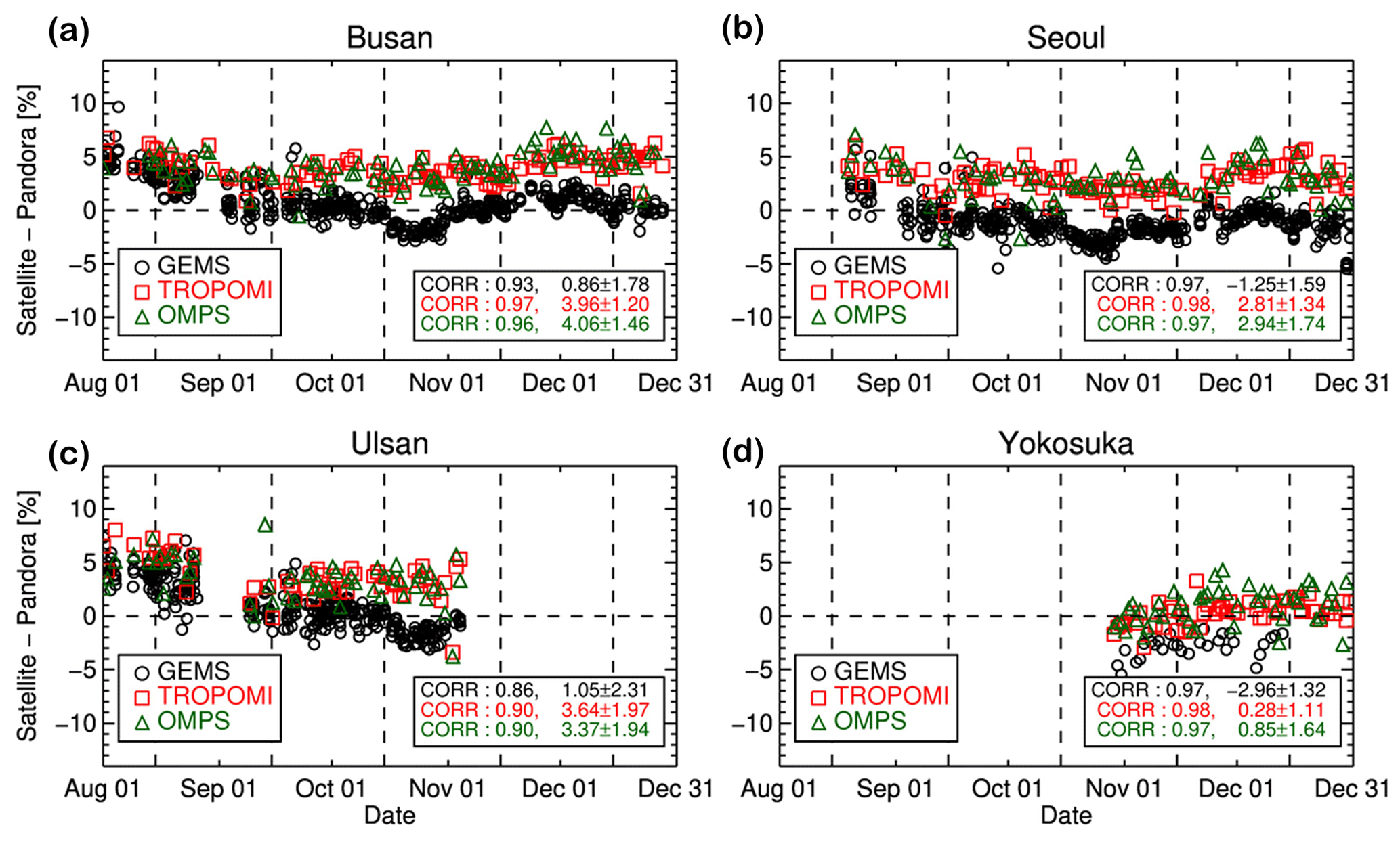
Figure 5 Time series of the daily percentage difference between Pandora and three satellite observations (with GEMS in black, TROPOMI in red, and OMPS in green) at Busan, Seoul, Ulsan, and Yokosuka from August to December 2020.

Table 2 The statistical metrics, including the correlation coefficient (R), root mean square error (RMSE), mean bias (MB), and mean standard deviation errors (MSE) comparing GEMS, TROPOMI, and OMPS with Pandora TCO at Busan, Seoul, Ulsan, and Yokosuka sites.

In Busan and Seoul, the mean bias (MB) is highest in August, at 3.5 % and 2.1 %, respectively. The MB then decreases from September to October before slightly increasing again in December. This seasonal pattern, although slightly overestimated in August, is similar to the MBs of TROPOMI and OMPS (Fig. 4b, c). GEMS overestimates by ∼0.85 % in Busan and underestimates by −1.25 % in Seoul when compared to Pandora over the entire analysis period. The significant bias observed in August does not appear to have a substantial impact on the average bias due to the reduced sample size resulting from cloud filtering. A comparison of the temporal distribution of GEMS and Pandora in Fig. 6 shows that GEMS can observe ozone daily variations that are nearly identical to Pandora within a similar range of errors, although GEMS has a bias of approximately 1 % compared to Pandora.

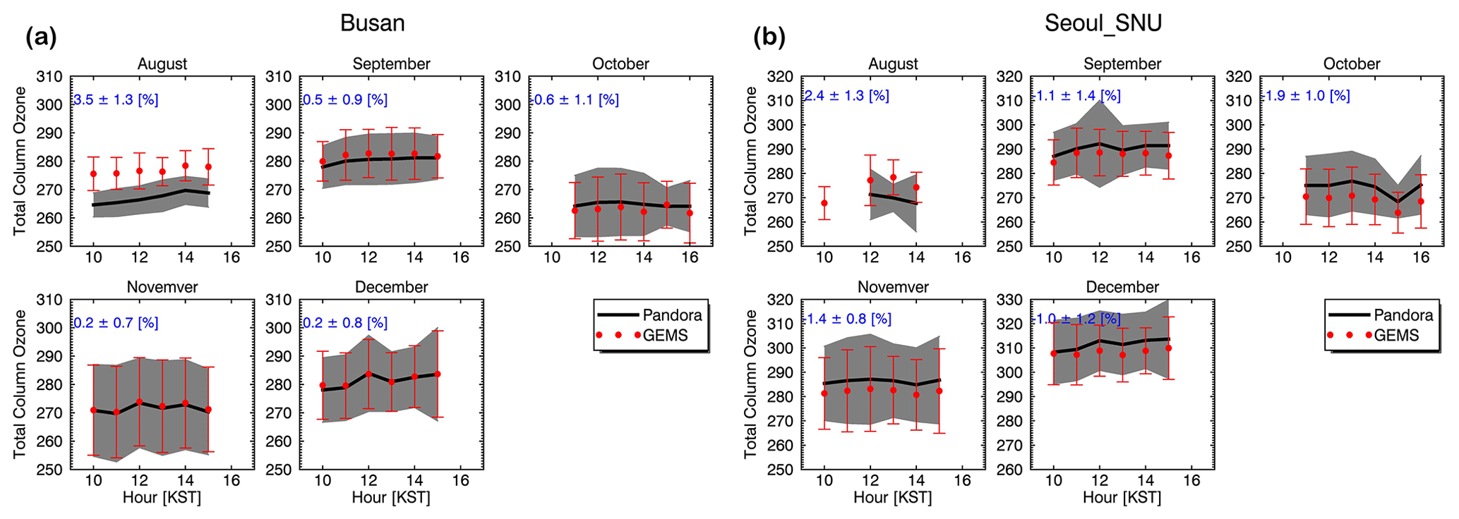
Figure 6 Time variation in the monthly mean values of GEMS (red-filled circles) and Pandora (a solid black line) in Busan and Seoul, covering the period from August to December. The standard deviation of Pandora TCO is represented by the gray shading, while the standard deviation of GEMS TCO is indicated by the bars.

3.3 Validation of GEMS total ozone with other satellites

Figure 7 shows the spatial distribution of TCO from GEMS, TROPOMI, and OMPS in the GEMS domain on 30 November 2020. This figure shows that the spatial distribution of TCO observed from the three satellites is in good agreement. It shows a typical ozone distribution pattern that increases from low to high latitudes.

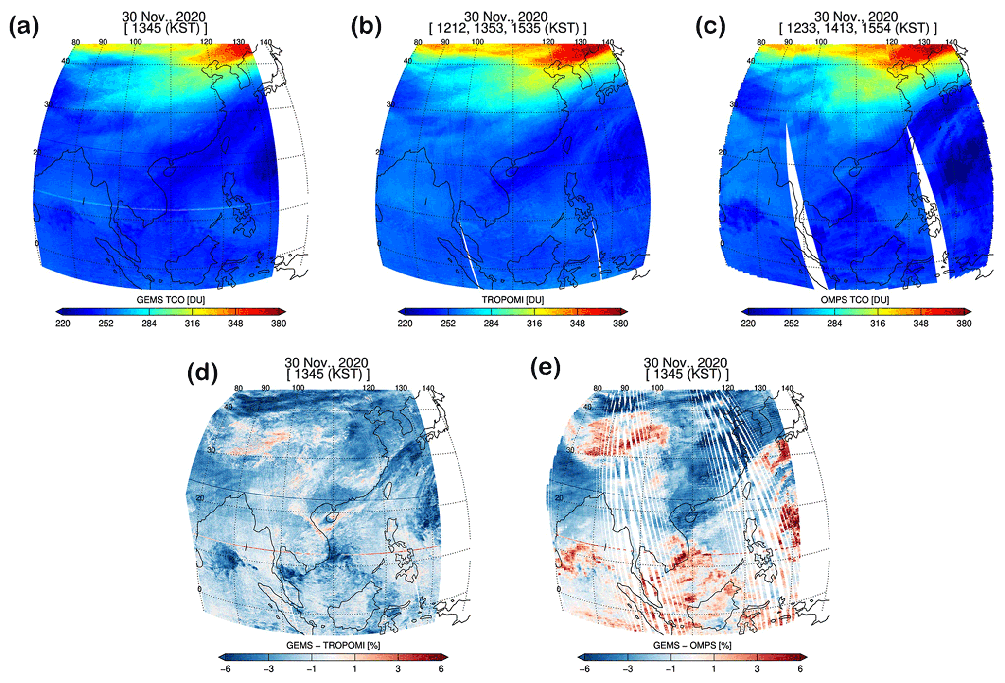
Figure 7 Maps of total column ozone from (a) GEMS, (b) TROPOMI, (c) OMPS, the (d) percentage difference between GEMS and TROPOMI, and the (e) percentage difference between GEMS and Pandora on 30 November 2020.

The distribution of wave patterns at high latitudes appears to be caused by atmospheric dynamics associated with meteorological phenomena. The horizontal striping in GEMS found around 10 and 20^∘ latitudes is an error caused by the bad pixels of the GEMS detector. These bad pixels are expected to be removed properly in the future by using an improved bad pixel mask variable in the GEMS level 1C data. Figure 7d and e display the bias maps of GEMS with respect to TROPOMI and OMPS, respectively. In Fig. 7d, GEMS TCO consistently shows a −3 % bias compared to the TCO from both satellites. However, Fig. 7e reveals a distinct positive bias of 2 %–3 % that is not evident in Fig. 7d. This positive bias is observed in the high reflectivity region associated with clouds, as indicated in Fig. 8. It is particularly pronounced in areas where OMPS measures significantly lower ozone, as shown in Fig. 7c. The strong anti-correlation between total ozone and clouds can be attributed to the difference in cloud height estimation methods used by the OMPS algorithm compared to GEMS and TROPOMI. OMPS derives cloud height from cloud climatology (Joiner and Vasilkov, 2006), while GEMS and TROPOMI retrieve cloud information from real-time-calculated cloud L2 products. The GEMS cloud retrieval algorithm employs the differential optical absorption spectroscopy (DOAS) method with the O₂–O₂ absorption band to retrieve effective cloud fraction, cloud centroid pressure, and cloud radiance fraction (NIER, 2020b). On the other hand, TROPOMI utilizes two algorithms for cloud retrieval, namely OCRA (Optical Cloud Recognition Algorithm) and ROCINN (Retrieval of Cloud Information using Neural Networks). OCRA estimates the cloud fraction by analyzing TROPOMI measurements in the ultraviolet and visible spectral regions, while ROCINN uses TROPOMI measurements within and around the oxygen A band in the near-infrared to retrieve cloud-top height (pressure) and optical thickness (albedo). For more detailed information on these cloud algorithms, refer to NIER (2020b) and Loyola et al. (2018). This difference in cloud height affects the TCO retrieval. Only ozone present above the cloud can be retrieved from the satellite's UV radiance over the cloudy scene, resulting in column ozone from the cloud height to the top of the atmosphere. The final TCO is calculated by adding the climatological ozone corresponding to the lower part of the cloud height. The OMPS climatology cloud height, as depicted in Fig. 8c, is remarkably lower than the cloud height retrieved by GEMS and TROPOMI in regions where actual clouds are present. Consequently, applying a lower cloud height leads to a reduced amount of ozone added below the cloud, resulting in a smaller OMPS TCO. On the other hand, a substantial decrease of approximately −5 % in the bias of GEMS for TROPOMI is evident in Fig. 7d, specifically in regions characterized by a high cloud fraction and altitude (Fig. 8). TROPOMI consistently indicates a cloud height of around 300 hPa, while GEMS retrieves a cloud altitude of approximately 500 hPa, revealing a significant disparity in the cloud height estimation. Although some differences in cloud altitudes are expected due to the use of different algorithms, the observed disparity in the cloud height between the two data sets is considerable. Therefore, further research is needed to investigate the impact of this significant difference in cloud height on the bias of GEMS for TROPOMI.

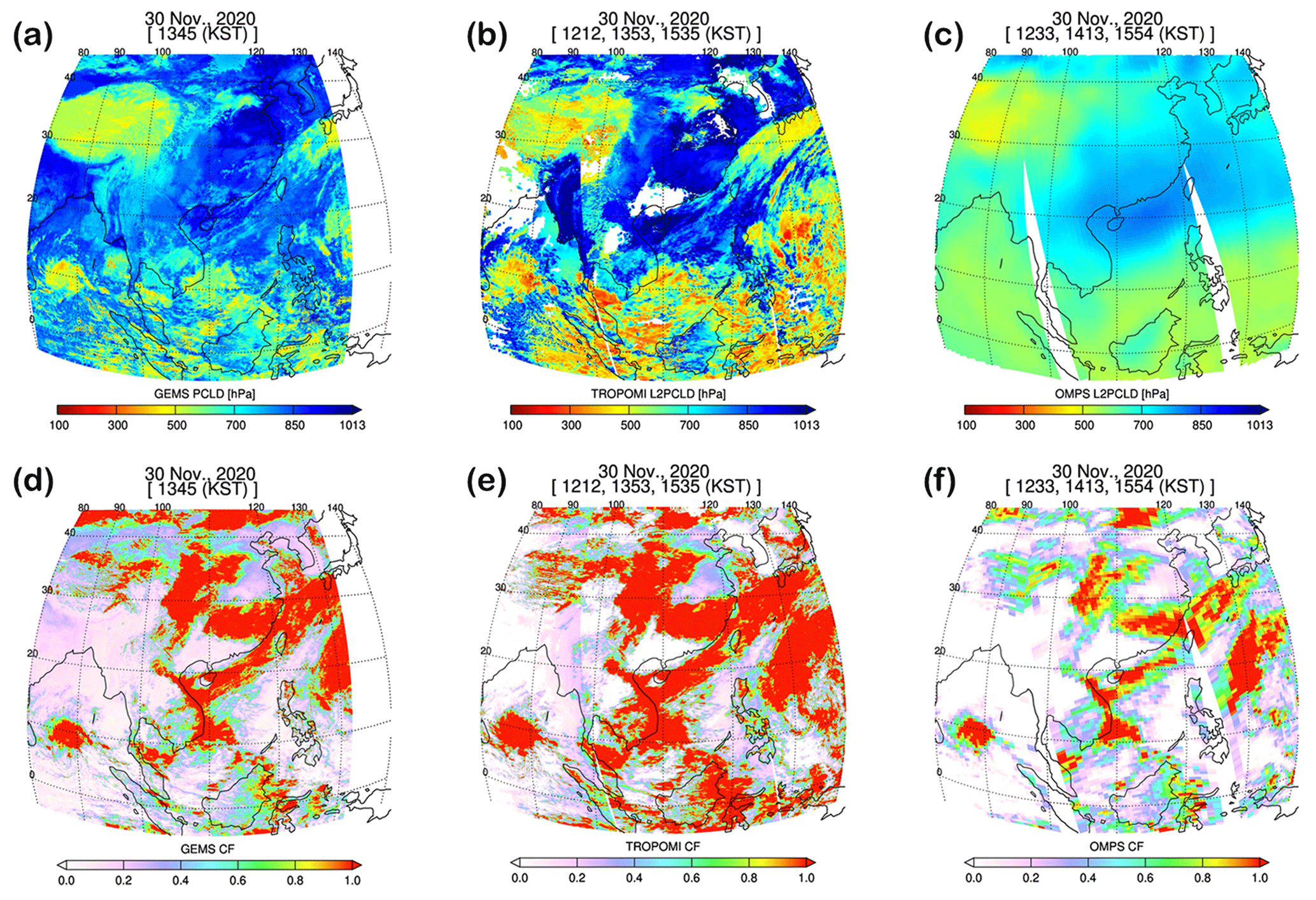
Figure 8 The spatial distribution of cloud pressure and cloud fraction obtained from GEMS, TROPOMI, and OMPS satellite observations on 30 November 2020. Panels (a), (b), and (c) display the maps of cloud pressure derived from GEMS, TROPOMI, and OMPS, respectively. Similarly, panels (d), (e), and (f) show the maps of cloud fraction obtained from GEMS, TROPOMI, and OMPS, respectively.

The histogram analysis was performed to compare the data sets with different spatial and temporal resolutions over the GEMS domain from August to December 2020 (Fig. 9). The histogram of all satellite data is similar to the normal distribution that shows good agreement with each other. Moreover, the distribution shape of GEMS, with an average of 267.3 DU, and TROPOMI, with an average of 272.6 DU, is very similar. However, the average of OMPS is smaller than the two-satellite data, and the peak is also tilted to a lower side than the average. This appears to be due to low ozone in cloudy pixels, as mentioned earlier.

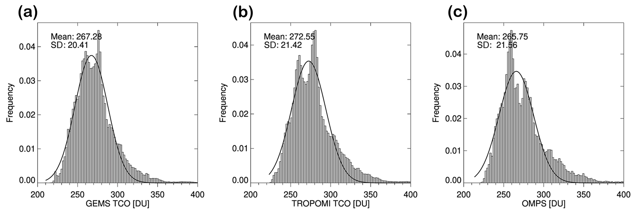
Figure 9 Histogram distribution of TCO from (a) GEMS, (b) TROPOMI, and (c) OMPS from 1 August to 31 December 2020, with their corresponding Gaussian fitting lines (black).

Since TROPOMI and OMPS have different observation times and fields of view relative to GEMS, it is necessary to match the spatial and temporal correspondence of the two data sets for quantitative comparison. For temporal consistency, the observation time difference between the polar orbit satellite and GEMS is shorter than 30 min. For spatial consistency, we selected the closest points within 10 km of the observation point of the two satellites. In addition, to use good-quality data for comparison, we used only data satisfying the quality control conditions presented in Table 3.

Table 3 Summary of validation data and methods.

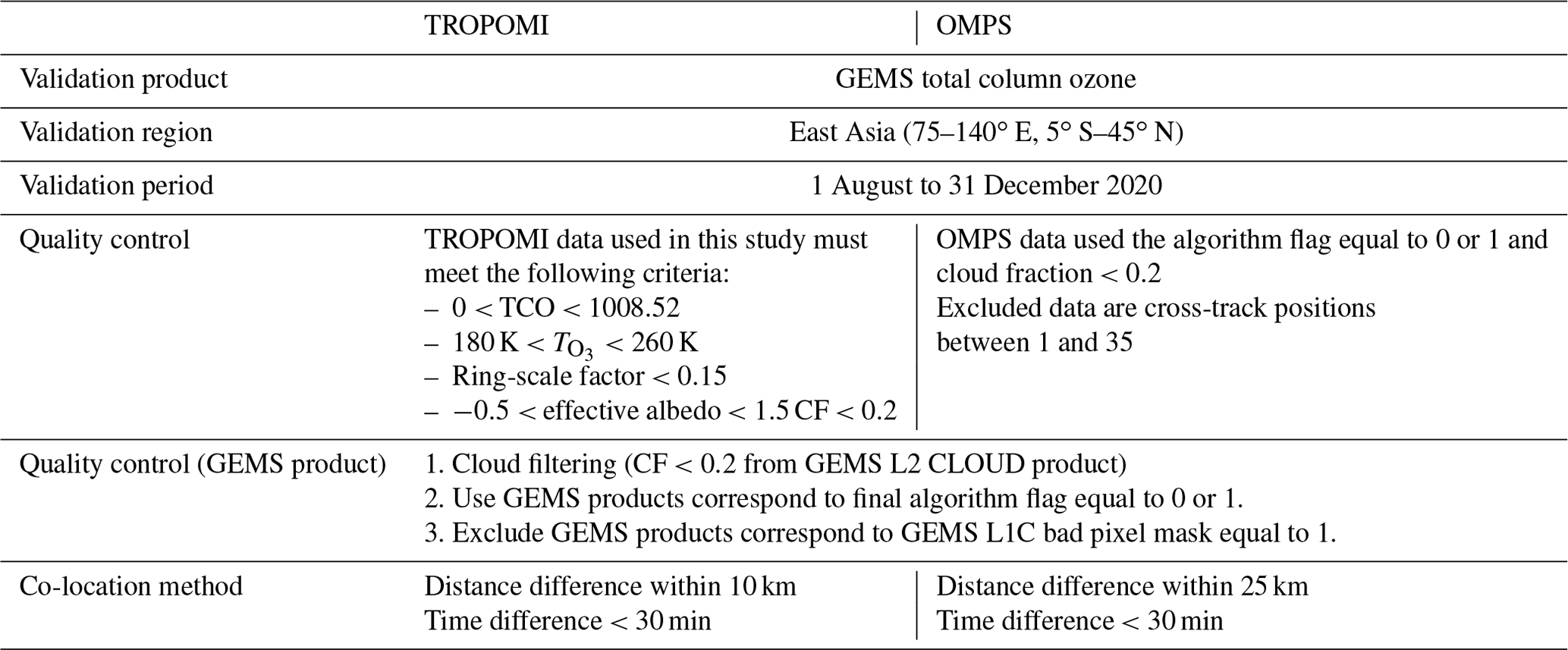
Figure 10 shows the quantitative comparison of GEMS TCO data with TROPOMI and OMPS TCO data for 5 months. It shows a high correlation coefficient greater than 0.98 and a low RMSE of less than 1.8 DU over clear-sky conditions. Compared to TROPOMI and OMPS, GEMS shows an underestimation, with a negative bias of −2.38 % (6.5 DU) and a standard deviation of 1.33 % and a negative bias of −2.17 % (6 DU) and a standard deviation of 1.57 %, respectively. It shows that the GEMS TCO agrees very well with the TROPOMI and OMPS TCO. However, in the red circle in Fig. 10a, a distinctly high value for the GEMS TCO is observed compared to the TROPOMI TCO. The reason for this is that we did not remove the amount of SO₂ ejected by the volcanic eruption of Nishinoshima (27.247^∘ N, 140.874^∘ E) in Japan between 1 and 5 August from the GEMS TCO, which resulted in a high GEMS TCO. There will be a further discussion about this in Fig. 11. Figure 10b shows the correlation between GEMS and OMPS. The abnormal deviation shown in Fig. 10a was not observed. Probably, the SO₂ influence was not removed because OMPS and GEMS use a similar algorithm.

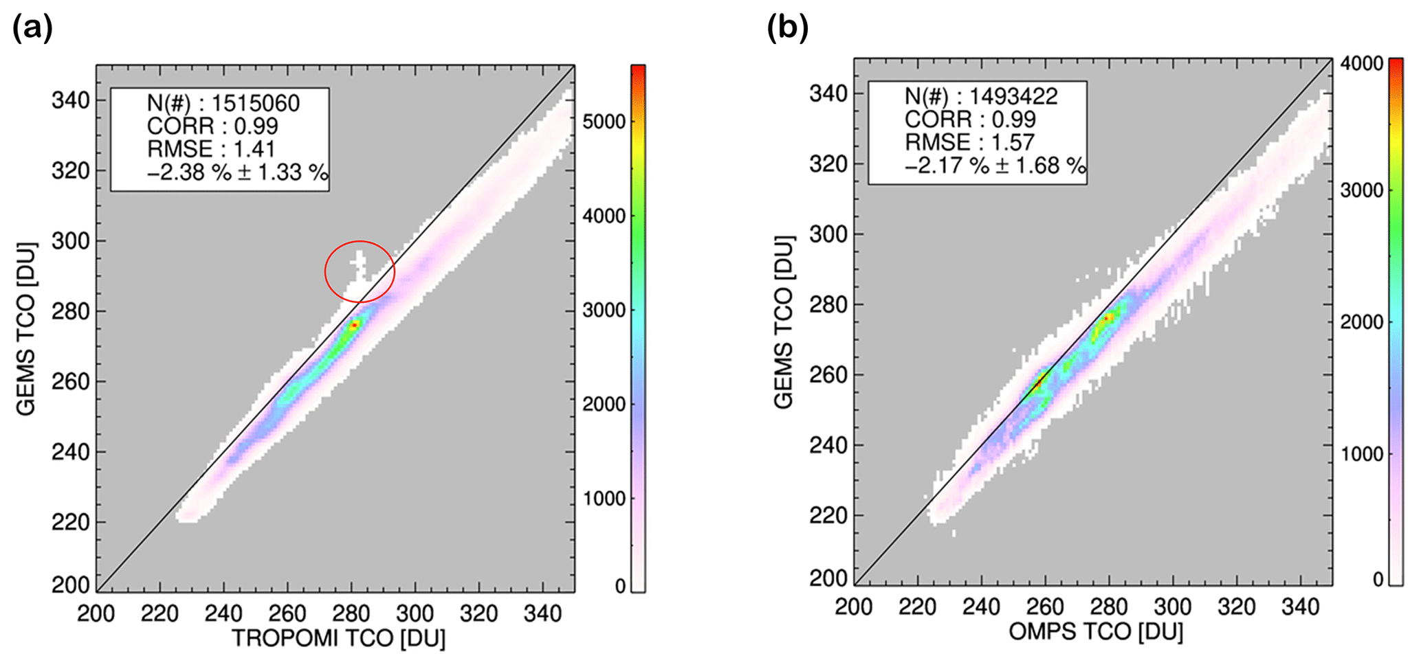
Figure 10 The comparison of GEMS TCO with (a) TROPOMI and (b) OMPS TCO from 1 August to 31 December 2020.

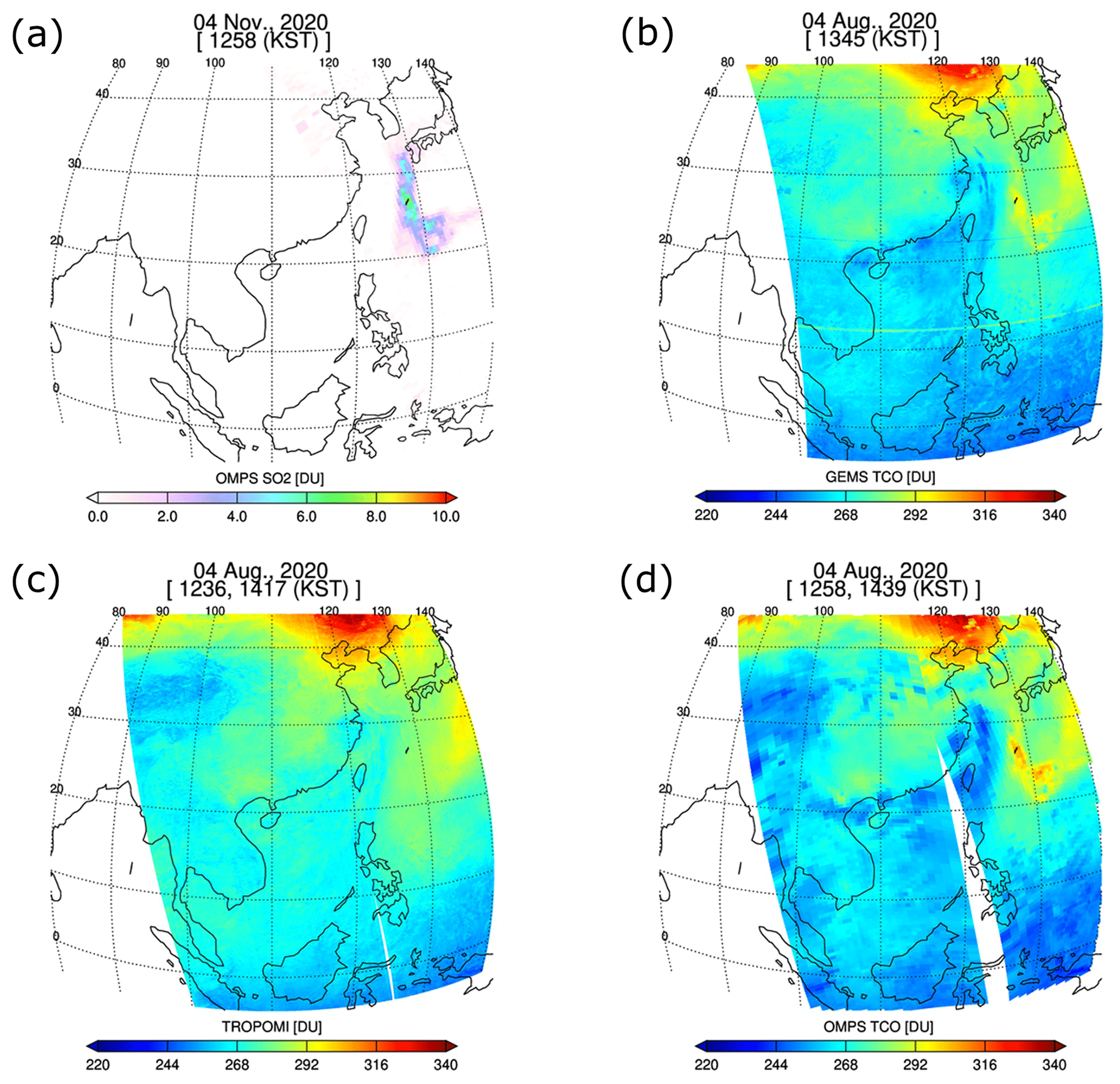
Figure 11 The map of (a) OMPS SO₂, (b) GEMS TCO, (c) TROPOMI TCO, and (d) OMPS TCO in the case of the volcanic eruption of Nishinoshima on 4 August 2020.

Figure 11 shows the distribution of satellite TCO and SO₂ on 4 August 2020, the day after the volcanic eruption of Nishinoshima in Japan. GEMS and OMPS show high TCO in regions with high SO₂ over 6 DU, but no distinctly high values from the TROPOMI TCO are observed. At a wavelength of 317.5 nm, which TOMS-based GEMS and OMPS algorithms use for ozone measurement, SO₂ also has a strong absorption line. Therefore, if the SO₂ effect was not properly removed, then TCO will be overestimated (Fisher et al., 2019; Krueger et al., 2008). However, since the TROPOMI direct-fitting algorithm derives the TCO using a 325–335 fitting window with a weak SO₂ absorption band, the SO₂ interference is negligible (Spurr et al., 2021).

Figure 12 shows the MBs between GEMS and TROPOMI and between GEMS and OMPS as a function of latitude for each month. GEMS–TROPOMI and GEMS–OMPS exhibit mean biases (MBs) of less than 1 % at low latitudes, but at midlatitudes, both MBs become negative and exhibit an increasingly negative dependence on latitude. Moreover, the dependency increases from August to December. The most significant change occurs at 40^∘ N, where the mean bias changes from approximately −1 % in August to −4 % in December.

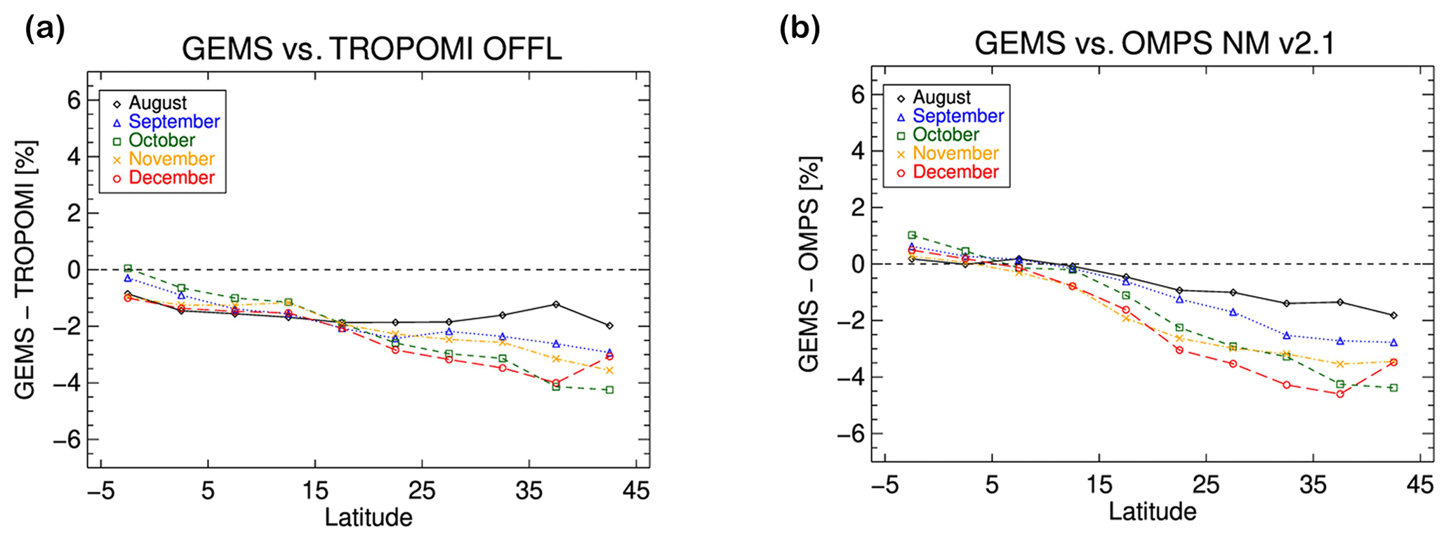
Figure 12 Mean bias in TCO between GEMS and TROPOMI (a) and GEMS and OMPS (b) as a function of latitude and months from August to December 2020. GEMS retrievals with the algorithm flag equal to 0, or 1 and the solar zenith angle (SZA) and view zenith angle (VZA) <70^∘. Symbols in the figure denote the months as follows: black diamonds are for August, blue triangles are for September, green squares are for October, yellow crosses are for November, and red circles are for December.

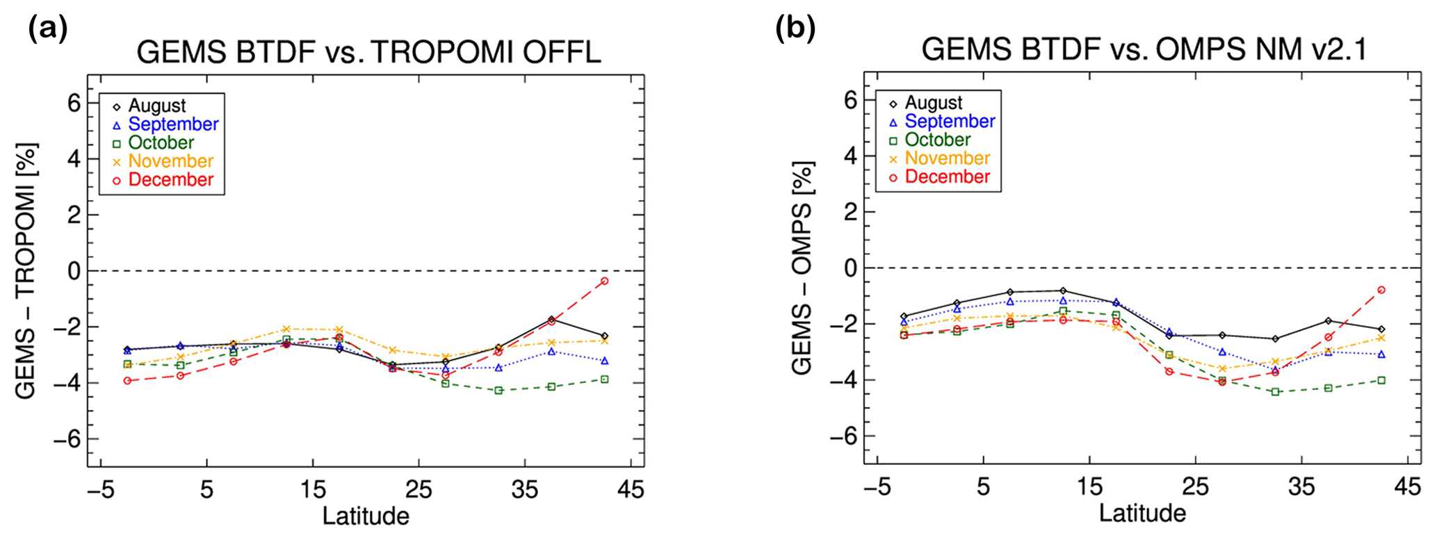
Figure 13 The mean bias (MB) in TCO between GEMS with BTDF correction and TROPOMI (a) and between GEMS with BTDF correction and OMPS (b) as a function of latitude and month from August to December 2020. Symbols in the figure denote the months as follows: black diamonds are for August, blue triangles are for September, green squares are for October, yellow crosses are for November, and red circles are for December.

Kang et al. (2022) noticed a problem in the GEMS level 1C irradiance because the bidirectional transmittance distribution function (BTDF) of the GEMS diffuser changes, depending on the Sun's illumination angle. They compared the daily GEMS irradiance to the solar reference spectrum, which was obtained from the convolution of the Royal Netherlands Meteorological Institute (KNMI) spectrum (Dobber et al., 2008) with the GEMS spectral response functions (SRFs; Kang et al., 2020). The GEMS irradiance was 20 % smaller than that of the reference spectrum and showed distinct spatial and seasonal variability. An empirical correction was applied to the BTDF to correct the GEMS irradiance by using the azimuthal angle and temporal variation in the GEMS instrument (Kang et al., 2022). We conducted an analysis on the GEMS TCO data calculated using the corrected GEMS irradiance data, following the same analysis method as shown in Fig. 12. Figure 13 shows a significant reduction in the MBs of TROPOMI and OMPS, which were 1 % and 0 %, respectively, at low latitudes, to −3 % and −2 %. The apparent decrease seen in midlatitudes in Fig. 12 was also significantly reduced. Although the overall negative bias compared to TROPOMI and OMPS remained consistent, the distinct negative trend seen in Fig. 12 for different latitudes and seasons was improved. However, for December, in the latitude range of 30 to 45^∘ N, there is a sudden positive bias trend increasing to −0.5 %, which is not found for different months. Therefore, to improve the accuracy of the GEMS ozone algorithm, more research is needed not only on bias correction but also on the performance of GEMS irradiance measurements.

4 Conclusion

The launch of the first geostationary environmental satellite, GEMS, has marked an important milestone in providing hourly monitoring of stratospheric ozone and air pollution, which significantly impact humans and ecosystems. This paper provides the atmospheric science community with the world's first assessment of GEMS total ozone retrieval performance and diurnal ozone variation. The algorithm used for GEMS is a more advanced version of its predecessor, the TOMS V8 algorithm. In addition to calculating total ozone, it has the advantage of providing ozone profile and retrieval error information.

To assess the performance of the GEMS algorithm, the hourly GEMS TCO was compared with the ground-based TCO measurements from Pandora that vary considerably through the day. The diurnal variation in the GEMS total ozone captures this variability and shows good agreement with that of Pandora. This indicates that the ozone undergoes significant diurnal change, primarily due to changes in stratospheric ozone, and it is evidence of why hourly ozone monitoring is important for tracking dynamic ozone changes. For further validation of GEMS TCO, we performed cross-comparisons between GEMS, Pandora TCO, and other satellite sensors, namely OMPS and TROPOMI. GEMS shows a high correlation of 0.97 and low RMSE compared to Pandora TCO at Busan and Seoul and exhibits daily variations in ozone that are highly consistent with the Pandora measurements, with a bias of approximately 1 %, despite exhibiting seasonal dependence in the mean bias of GEMS–Pandora. The comparison of GEMS TCO data with TROPOMI and OMPS TCO data shows a high correlation of 0.99 and low RMSE but a negative bias of −2.38 % and −2.17 %, respectively, with standard deviations of 1.33 % and 1.57 %. The influence of SO₂ from volcanic eruptions is not properly removed in some regions, leading to GEMS overestimating TCO in those areas, similar to OMPS. The mean biases of GEMS TCO data with TROPOMI and OMPS TCO are less than 1 % at low latitudes but become negative at midlatitudes, with an increasingly negative dependence on latitude. Furthermore, this dependence becomes more prominent from summer to winter. GEMS solar irradiance is 20 % lower than the Dobber et al. (2008) reference spectrum and shows distinct spatial and seasonal variability. An empirical correction applied to the GEMS irradiance data improved the dependence of the mean bias on the season and latitude, but a consistent bias still remains, and a marginal positive trend was observed in December.

Improvements in the GEMS sensor characterization should improve the quality of the GEMS total ozone retrieval. Nevertheless, the results presented in this work that have been achieved thus far are a meaningful scientific advancement by providing the first validated, hourly UV ozone retrievals from a satellite in a geostationary orbit. This experience can be used to advance research with future geostationary environmental satellite missions, including TEMPO, which was launched on 7 April 2023, and Sentinel-4, which is scheduled to be launched in 2024.