the Creative Commons Attribution 4.0 License.
the Creative Commons Attribution 4.0 License.
 | 08 Dec 2023
Difference spectrum fitting of the ion–neutral collision frequency from dual-frequency EISCAT measurements
Florian Günzkofer
Gunter Stober
Dimitry Pokhotelov
Yasunobu Miyoshi
Claudia Borries
The plasma–neutral coupling in the mesosphere–lower thermosphere strongly depends on the ion–neutral collision frequency across that region. Most commonly, the collision frequency profile is calculated from the climatologies of atmospheric models. However, previous measurements indicated that the collision frequency can deviate notably from the climatological average. Direct measurement of the ion–neutral collision frequency with multifrequency incoherent scatter radar (ISR) measurements has been discussed before, though actual measurements have been rare. The previously applied multifrequency analysis method requires a special simultaneous fit of the two incoherent scatter spectra, which is not possible with standard ISR analysis software. The difference spectrum method allows us to infer ion–neutral collision frequency profiles from multifrequency ISR measurements based on standard incoherent scatter analysis software, such as the Grand Unified Incoherent Scatter Design and Analysis Package (GUISDAP) software. In this work, we present the first results by applying the difference spectrum method. Ion–neutral collision frequency profiles obtained from several multifrequency EISCAT ISR campaigns are presented. The profiles obtained with the difference spectrum method are compared to previous collision frequency measurements, both from multifrequency ISR and other measurements, as well as results from empirical and comprehensive atmosphere models. Ion–neutral collision frequency measurements can be applied to improve first-principle ionospheric models.
- Article
(2221 KB) - Full-text XML
- BibTeX
- EndNote


The magnetospheric current system is closed in the ionospheric dynamo region at approximately 80–130 km altitude due to the maxima of transverse conductivities at these altitudes (Baumjohann and Treumann, 1996). These maxima occur due to the special relations between ion/electron–neutral collision frequencies (νin, νen) and ion/electron gyrofrequencies (ωi, ωe). In the dynamo region, electrons are coupled with the Earth's magnetic field lines (νen≪ωe), whereas ions are decoupled due to frequent collisions with neutral particles (νin≫ωi) (Brekke et al., 1974). Due to the transition from a collisional to a collisionless plasma, the dynamo region is also often referred to as the ionospheric transition region, and we will use both terms synonymously.
Knowledge of the vertical collision frequency profiles is essential for understanding and predicting ionospheric conductivities and their impact on the atmosphere–ionosphere coupling, e.g., due to the Joule dissipation of Pedersen currents. The impact of ion–neutral collisions on the diffusion of meteor trails makes direct collision frequency measurements important for the analysis of meteor radar data as well (Stober et al., 2023). Neutral wind measurements with incoherent scatter radars (ISRs) also require a priori knowledge of the collision frequencies in the dynamo region (e.g., Brekke et al., 1973; Nozawa et al., 2010; Günzkofer et al., 2022). νin and νen can be calculated by leveraging simplified and idealized relations derived by Chapman (1956) for the ion–neutral collision frequency,
and by Nicolet (1953) for the electron–neutral collision frequency,
In Eqs. (1) and (2), nn and ni are neutral and ion volume densities per cubic centimeter, respectively; A is the mean atomic mass number; and Te is the electron temperature (Kelly, 2009). However, the neutral density nn is often taken from empirical atmosphere models such as NRLMSISE-00 (Picone et al., 2002), which introduce a major source of uncertainty when estimating the collision frequencies from the above equations. The relations in Eqs. (1) and (2) are derived assuming ion–neutral and electron–neutral collisions as elastic rigid-sphere collisions (Nicolet, 1953; Chapman, 1956).
There are multiple approaches for direct or indirect measurements of collision frequencies in the ionosphere.
It was shown that it is possible to infer the ion–neutral collision frequency utilizing line-of-sight ion velocity vi measurements from ISRs (Nygren et al., 1987). Such an indirect measurement method, however, requires specific conditions and assumptions and is therefore only applicable above ∼106 km altitude and for electric fields E≳20 mV m−1 (for a more detailed discussion of this method, see Oyama et al., 2012, and references therein). The ion–neutral collision frequency can also be directly inferred from ISR measurements due to its impact on the incoherent scatter spectrum (e.g., Dougherty and Farley, 1963; Farley, 1966; Grassmann, 1993a). However, the shape of the incoherent scatter spectrum is ambiguous towards changes in the collision frequency and changes in ion and electron temperatures Ti and Te. The ambiguity can be overcome by assuming Te=Ti; however, this assumption has to be considered carefully. A summary and discussion of multiple studies that followed this approach with the EISCAT ISR can be found in Nygrén (1996). In these studies, it was generally assumed that at high latitudes Te=Ti is valid for low-geomagnetic-activity conditions and below ∼110 km altitude.
The ion–neutral collision frequency can also be inferred from two incoherent scatter spectra obtained with simultaneous measurements of two ISRs, with well-separated transmitter frequencies. This is possible at the EISCAT site in Tromsø, Norway, where two ISRs with transmitter frequencies of 929 and 224 MHz are operated. Many methods to analyze EISCAT dual-frequency measurements to obtain ion–neutral collision frequencies have been suggested (Grassmann, 1993b). However, actual dual-frequency measurements have been scarce, and only one study performed an analysis to derive collision frequencies (Nicolls et al., 2014). It should be noted that the EISCAT ISR systems are the only ones capable of performing dual-frequency measurements. In their study, Nicolls et al. (2014) followed an approach suggested by Grassmann (1993b) that requires the simultaneous fitting of both measured spectra to obtain the optimum parameters from the combined fit. This method requires a customized ISR spectrum fitting algorithm and, therefore, cannot be applied within the standard EISCAT analysis software, Grand Unified Incoherent Scatter Design and Analysis Package (GUISDAP). An alternative method suggested by Grassmann (1993b) is the so-called difference spectrum fitting, which combines the spectra after the standard ISR analysis.
In this work, the applicability of the difference spectrum fitting for the measurement of ion–neutral collision frequencies using the two EISCAT ISR systems (UHF and VHF) is demonstrated. We compare the obtained profiles to the results from Nicolls et al. (2014) as well as to other collision frequency measurement methods. The vertical profile of neutral particle density can be inferred from the measured ion–neutral collision frequency, either by applying Eq. (1) or any other collision frequency relation, though most require certain assumptions on the atmospheric composition across the ionospheric dynamo region. The neutral density profiles can be partially validated by meteor radar measurements in the mesosphere–lower thermosphere (MLT) region (Stober et al., 2012, 2014; Dawkins et al., 2023) or by leveraging occultation measurements from satellites of X-ray sources such as the Crab Nebula (Katsuda et al., 2023). Since measurements of atmospheric densities in the ionospheric dynamo region are very rare, dual-frequency ISR measurements allow us to obtain the valuable information required for the validation of atmosphere models. The results of our analysis will be compared to several atmosphere models.
2.1 EISCAT UHF and VHF radar
The EISCAT Scientific Association operates an ultrahigh-frequency (UHF) and a very-high-frequency (VHF) ISR with frequencies of 929 and 224 MHz, respectively, near Tromsø, Norway (69.6∘ N, 19.2∘ E) (Folkestad et al., 1983). The UHF transmitter operates with a power of about 1.5–2 MW. The dish used for transmitting and receiving is 32 m in diameter. The VHF transmitter has a peak power of about 1.5 MW, and the co-located VHF receiver antenna consists of four rectangular (30 m × 40 m) dishes. To perform the dual-frequency analysis, both systems have to be operated at the same time in the same radar mode. A summary of all EISCAT experimental modes can be found in Tjulin (2021). In this work, multiple EISCAT campaigns are analyzed.
2.1.1 August 2013 and September 2021 campaigns
Nicolls et al. (2014) planned and analyzed the EISCAT campaign on 29 August 2013 from 07:00–11:00 UTC. The measurements were conducted with both ISRs operating in the beata radar mode, pointing to the geographical north with an elevation of 45∘. This experiment mode allows measurements from about 80 to 500 km altitude, with a vertical resolution of 5–10 km in the transition region.
On 27 September 2021 from 08:00–12:00 UTC, a dual-frequency EISCAT campaign was conducted leveraging the same radar mode and geometry.
2.1.2 October 2022 campaign
On 13 October 2022 from 08:00–13:00 UTC, a dual-frequency EISCAT campaign was conducted in the manda zenith experiment mode, also known as the EISCAT Common Programme (CP) 6. As the name suggests, the radar was pointed to the local zenith at 90∘ elevation. This mode allows measurements between about 70 and 200 km, with a vertical resolution of about 0.4–10 km in the transition region.
2.2 NRLMSIS
Since measurements of ion–neutral collision frequencies are rarely available, climatological profiles from empirical atmosphere models often have to be assumed. One application of such profiles is the derivation of neutral winds from ISR ion velocity measurements (e.g., Nozawa et al., 2010; Günzkofer et al., 2022). The mass spectrometer and incoherent scatter radar (MSIS) model (Hedin, 1991) is available in many different versions and is one of the most commonly used empirical atmosphere models. In this paper, we will use empirical atmosphere models both for comparison to measurement data and to obtain profiles of neutral atmosphere parameters that are not available from measurements. Two MSIS versions are applied, NRLMSISE-00 (Picone et al., 2002) and NRLMSIS 2.0 (Emmert et al., 2021).
2.3 GAIA
The Ground-to-topside model of Atmosphere and Ionosphere for Aeronomy (GAIA) is a global circulation model giving neutral dynamics for all altitudes from the ground up to ∼600 km (Jin et al., 2012). The GAIA output was compared and verified with experimental data from numerous different apparatuses for time spans up to several decades. A comparison to meteor radar wind climatologies at the MLT can be found in Stober et al. (2021). GAIA simulations are nudged up to ∼30 km altitude to the Japanese Reanalysis data (JRA-25/55; Kobayashi et al., 2015). In this study, we use data from GAIA on a grid with a resolution of 1∘ in latitude and 2.5∘ in longitude. The GAIA output is available with a vertical resolution of of the scale height.
In this section, we describe the difference spectrum fitting method equivalent to Grassmann (1993b), though we changed the notation of some variables. Furthermore, results from multiple EISCAT campaigns are presented. As mentioned in Sect. 1, the main advantage of this method over other approaches described in Grassmann (1993b) is that it can be applied on top of already existing ISR analysis. It, therefore, does not require detailed knowledge of the ISR spectrum fitting process. For all EISCAT data presented in this paper, the fitting of ISR spectra is done with Version 9.2 of GUISDAP (Lehtinen and Huuskonen, 1996). As a priori guesses for the spectra fits, GUISDAP utilizes the climatology models MSIS and IRI. For a weak signal-to-noise ratio, the fitting returns the a priori climatology parameter profiles. However, for a sufficiently good signal quality, the choice of a priori climatology has no impact on the fitted parameters.
In the following, we will distinguish between measured spectra S(ωx+δω) and theoretical spectra with the transmitter frequency ωx. During the fitting process, the measured incoherent scatter spectra S(ωVHF+δω) and S(ωUHF+δω) are saved. The measured VHF spectrum can be scaled to UHF frequencies, knowing the ratio for the EISCAT systems. According to Grassmann (1993b), the scaled VHF spectrum is equivalent to a UHF incoherent scatter spectrum for the scaled parameters ξ2⋅Ne and ξ⋅νin, meaning,
The UHF spectrum and scaled VHF spectrum can be combined into a single difference spectrum,
where the additional parameter β is included to account for technical differences between the UHF and VHF radars. As described in Grassmann (1993b), β is determined at sufficiently high altitudes, where νin=0 and therefore can be assumed. It can be seen from Eq. (4) that the two radar frequencies have to be distinctly different. If ξ is close to 1, the difference spectrum would be in the range of the measurement uncertainties, and no information could be inferred from it.
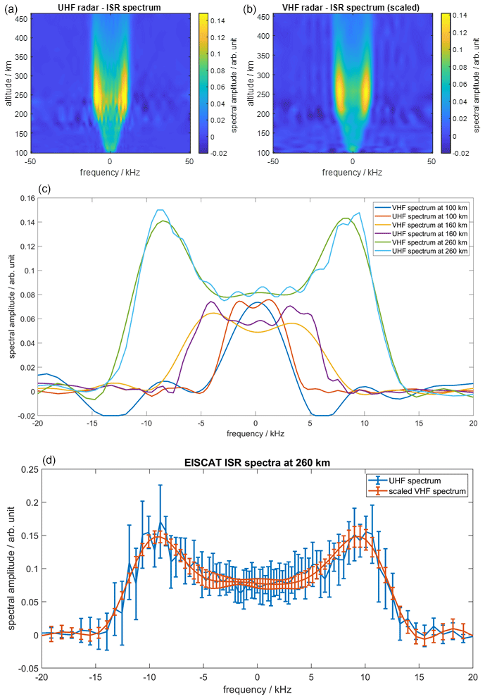
Figure 1EISCAT UHF (a) and scaled VHF (b) spectra measured on 27 September 2021. (c) Comparison of spectra at 260, 160, and 100 km altitudes. It can be seen how the incoherent scatter spectrum changes shape with increasing collision frequency. (d) The UHF and scaled VHF at 260 km altitude with statistical uncertainties over a range of 10 min.
Figure 1 compares the measured UHF spectrum (top left) with the VHF spectrum after scaling (top right). It can be seen that the spectral intensity maximizes at approximately 200–300 km altitude. β is therefore determined at about 260 km, where the plasma can be assumed as collisionless. Figure 1 (middle) shows the UHF and VHF spectra at three selected altitudes: 260 km, where β is determined, and at two altitudes in the upper and lower transition regions at 160 and 100 km, respectively. At 260 km, both spectra exhibit the typical ISR double-peak shape. As described by Grassmann (1993b), the double-peak shape disappears with increasing νin, first for the VHF spectrum and at lower altitudes for the UHF spectrum as well. In Fig. 1 (bottom), the UHF and scaled VHF spectra at 260 km altitude are shown for a 10 min interval, with the statistical uncertainty throughout that period. Whether the uncertainties are caused by a variation of the ionospheric plasma parameters within this interval or are the result of uncertainties of the incoherent scatter measurements cannot be conclusively determined. The measured difference spectrum is calculated according to Eq. (4) and fitted to the theoretical difference spectrum function,
It can be seen from Eq. (3) that the scaled VHF spectrum corresponds to a UHF spectrum with scaled collision frequency ξ⋅νin. The parameters Ti and Te are not affected by the frequency scaling. Therefore, the difference spectrum in Eq. (5) allows us to infer νin, Ti, and Te without ambiguity or any further assumptions. Figure 2 shows the vertical profile of the ion–neutral collision frequency at 90–150 km altitude for 27 September 2021 from 08:00–12:00 UTC.
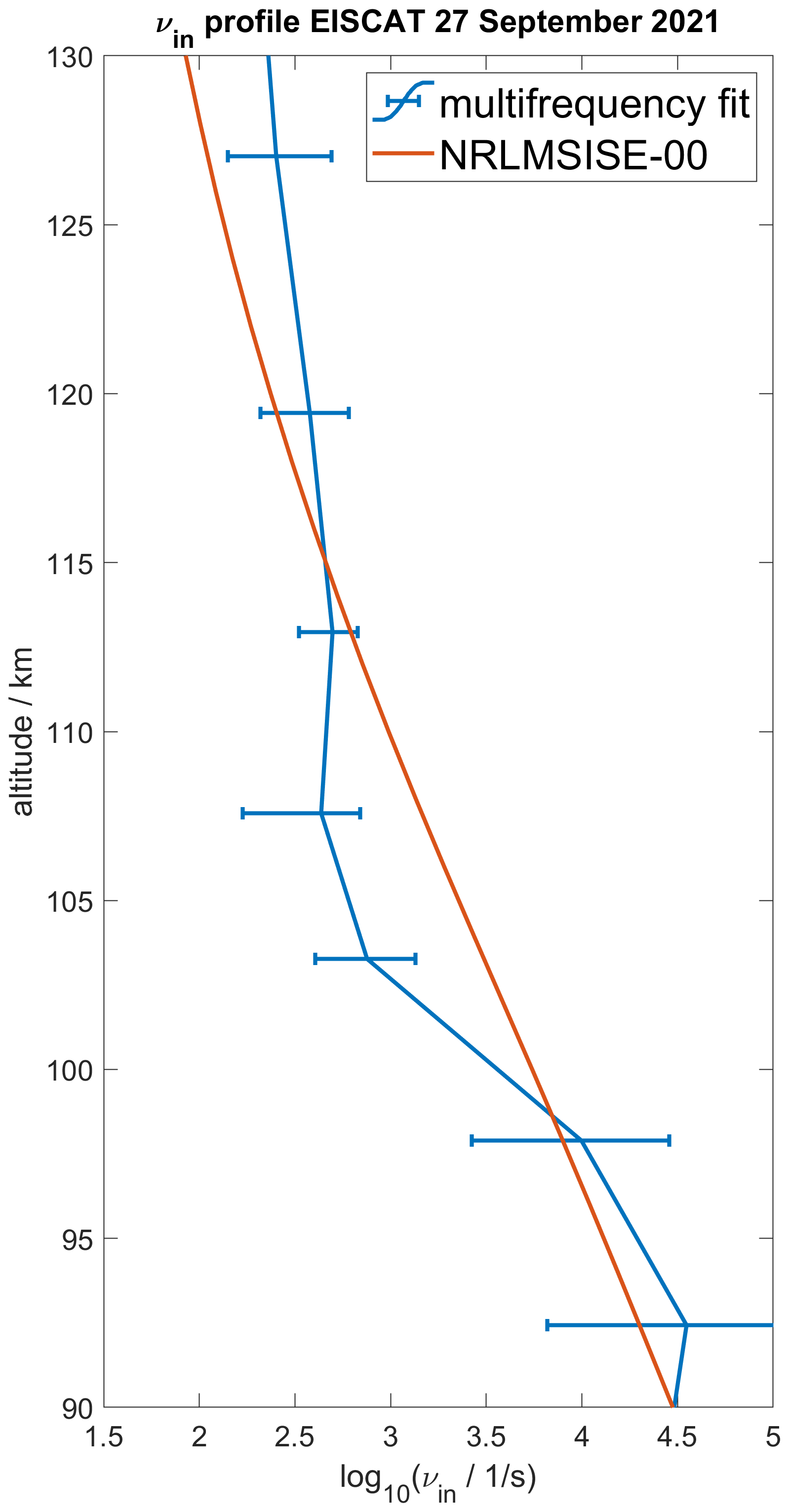
Figure 2Median vertical profile of νin on 27 September 2021 from 08:00–12:00 UTC. One profile fit is performed every 60 s, and the error bars mark the statistical interquartile range. For comparison, a climatological median profile is calculated from the NRLMSISE-00 model.
The fitted ion–collision frequency profile shows reasonable values across the whole ionospheric transition region. The error bars shown in Fig. 2 mark the upper and lower quartile of the geophysical variation during the 4 h of measurement. The uncertainties of the ISR spectra are not obtained during the GUISDAP fitting process. However, it can be assumed that for a large enough signal-to-noise ratio the geophysical variation exceeds the effects of the ISR spectrum uncertainty. Below ∼120 km, the fitted profile oscillates around the climatological mean calculated with Eq. (1) from the NRLMSISE-00 neutral density. At altitudes above 120 km, the fitting method shows a general tendency to larger collision frequencies in comparison with the NRLMSISE-00 model.
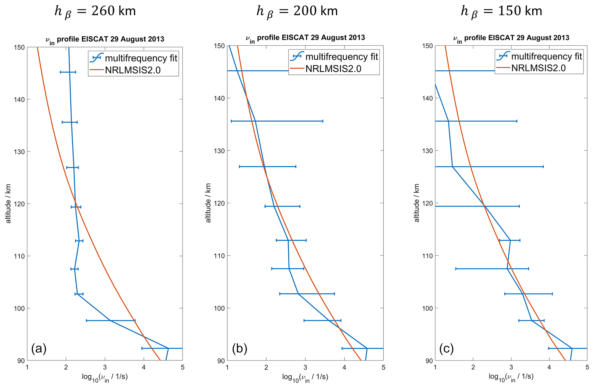
Figure 3νin profiles for three different hβ. The β parameter was determined at 260 km altitude in panel (a), 200 km in panel (b), and 150 km in panel (c).
As mentioned earlier, there is only one previous multifrequency ISR experiment. The EISCAT campaign from 27 September 2021 was run in the same radar mode as the experiment on 29 August 2013. This allows us to directly apply the developed difference spectrum fitting method to these measurements and compare them to the results shown in Nicolls et al. (2014). However, the fitted profiles for this campaign show a strong dependence on which altitude hβ is used to determine the β parameter. The fitted νin profiles for three different altitudes hβ are shown in Fig. 3 for 20 August 2013 from 07:00–11:00 UTC.
The hβ=260 km profile deviates strongly from the climatological NRLMSIS profile and shows a nearly constant collision frequency at ∼110–150 km altitude. This is unexpected and has to be discussed carefully. The two profiles for hβ=200 km and hβ=150 km show more resemblance to the climatological average, though the propagated uncertainties are larger compared to the first profile. The hβ=150 km profile is also very similar to the profile shown in Nicolls et al. (2014). The vertical profiles of the β parameter versus the altitude where it is determined are shown in Fig. 4 for the two campaigns on 29 August 2013 and 27 September 2021.
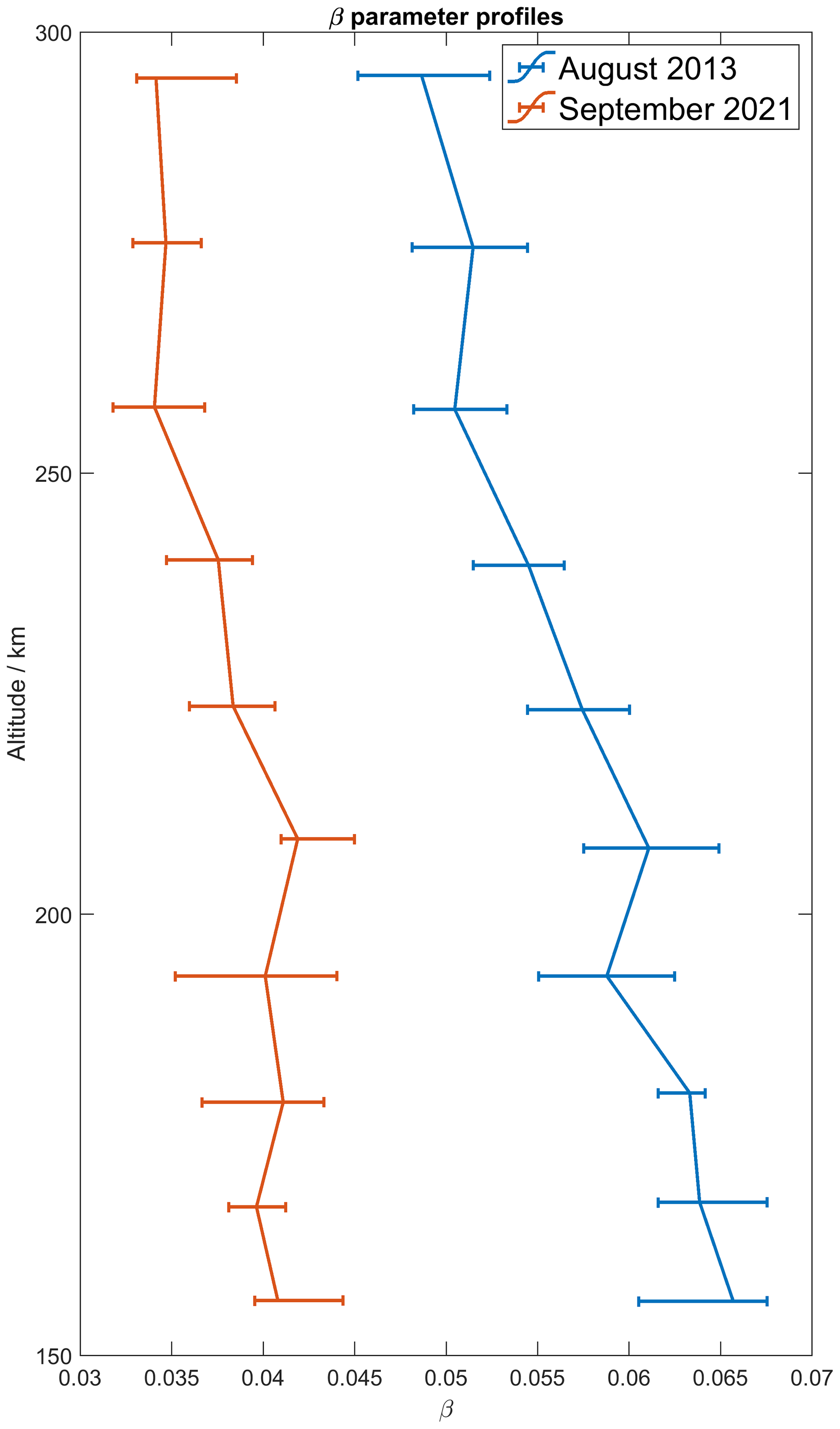
Figure 4Profiles of the β parameter vs. the altitude where it has been determined for the EISCAT campaigns on 29 August 2013 and 27 September 2021.
Since the β parameter does not exhibit a general trend over the timescale of a single measurement campaign, Fig. 4 shows the median β profile for each of the two campaigns. It can be seen that the β parameter has changed in the time between the two campaigns. The variation with altitude is more pronounced for the August 2013 campaign, with an altitude change rate of km−1. For the September 2021 campaign, the gradient of the β profile is km−1. This might explain the distinct changes in the August 2013 νin profile shown in Fig. 3. However, what causes these changes in β with altitude remains to be discussed.
The third dual-frequency EISCAT campaign was conducted on 13 October 2022. For this campaign, a different radar mode was applied, which enables a better vertical resolution in the MLT region in exchange for a reduced absolute vertical coverage. Figure 5 shows the νin profile obtained from simultaneous manda zenith measurements, with the EISCAT UHF and VHF radars at 80–100 km altitude. A climatology profile from the NRLMSISE-00 model is shown as well as the a priori collision frequency profile applied during the difference spectrum fit. The a priori profile is obtained from the νin values given by the single-frequency GUISDAP analysis of the UHF measurements. The single-frequency result is close to a climatological profile with slightly lower values than the NRLMSISE-00 profile.
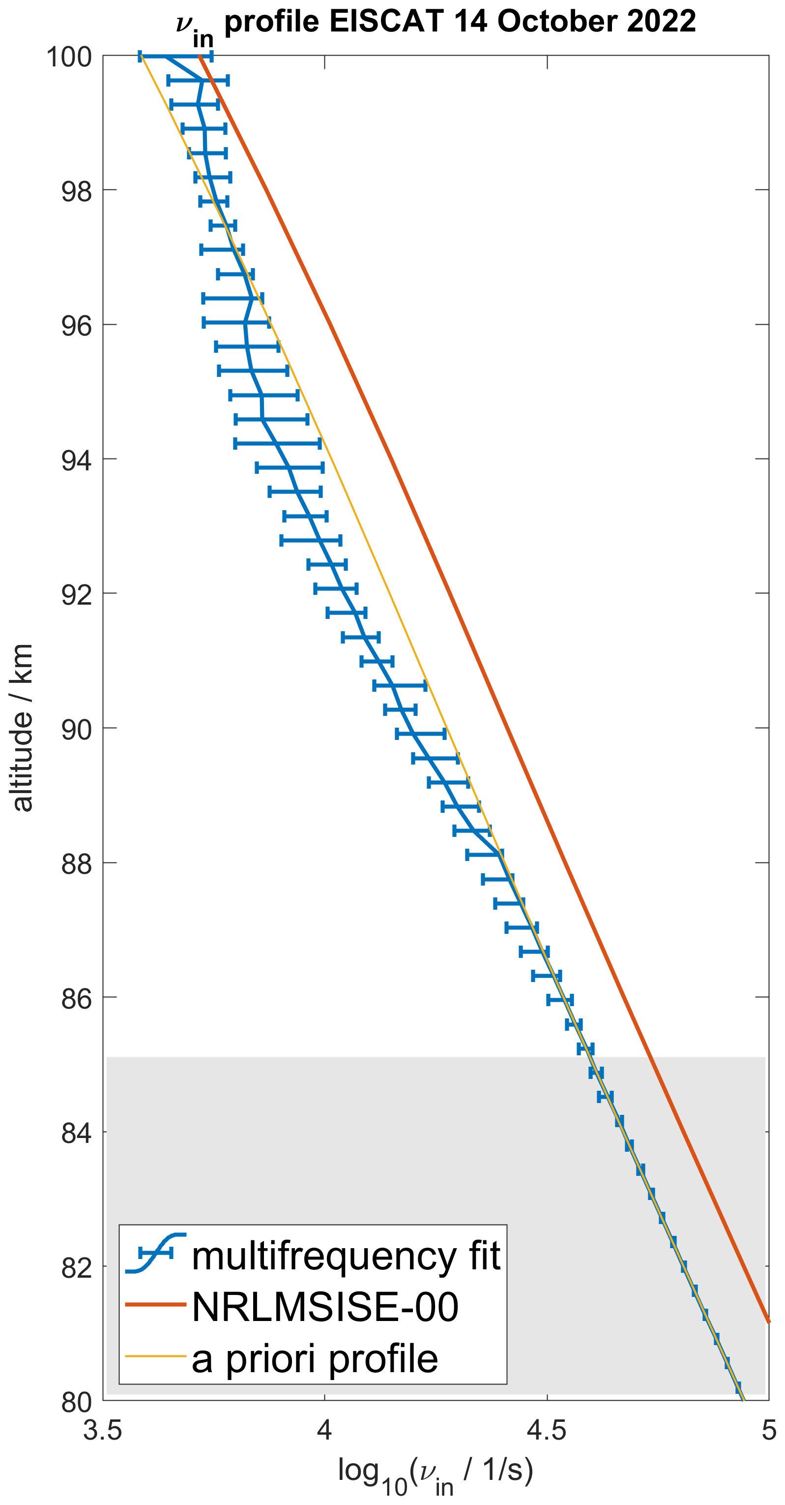
Figure 5High-altitude resolution νin profile from EISCAT manda zenith measurements. The grey area marks the altitude where the dual-frequency fit did not converge.
It can be seen in Fig. 5 that the dual-frequency fit has almost no measurement response at altitudes ≲85 km, where the fitted profile is identical to the a priori profile. Thus, at those altitudes, there is not enough signal-to-noise ratio left to drive the profile away from the a priori profile.
Equation (1) describes how the ion–neutral collision frequency can be calculated from the neutral particle density nn and the mean ion mass A, assuming the mean ion mass equals the mean neutral atom/molecule mass. Equation (1) assumes ion–neutral collisions as rigid-sphere collisions (Chapman, 1956) and allows us to calculate the neutral particle densities from the measured ion–neutral collision frequency profiles. Instead of rigid-sphere collisions, the ion–neutral collision frequency can be calculated assuming Maxwell collisions (Dalgarno et al., 1958). When calculating the neutral particle density with this method, it is necessary to know the relative abundance of each neutral particle species as well as the neutral particle polarizability, which can be found in, e.g., Schunk and Nagy (2009). Since this method evaluates the collisions for each ion and neutral species separately, resonant ion–neutral interactions between the same species have to be considered. The parameters for resonant collisions are available in Schunk and Nagy (2009) as well. Resonant collision parameters depend on the ion temperature Ti, which is available from the EISCAT measurements.
Figure 6 shows two neutral particle density profiles calculated with different collision models compared to two profiles directly taken from neutral atmosphere models. The neutral densities are calculated from the ion–neutral collision frequency profile obtained for the 29 August 2013 campaign with the β parameter determined at 150 km altitude. The uncertainties shown in Fig. 6 are predominantly caused by the uncertainties of the collision frequency profile in Fig. 3. The geophysical variation of the model's neutral atmosphere background is comparably small, and, therefore, the uncertainties are the same for all measured profiles. The profile calculated from the rigid-sphere collision formula in Eq. (1) assumes the mean particle mass A as given by GAIA, which spans a range of ∼26–29 amu across the transition region. Neutral density profiles calculated from Eq. (1) for the A profile from the NRLMSIS 2.0 model or a constant A=30.5 amu profile, which is a previously used assumption for the transition region (e.g., Nozawa et al., 2010), are nearly identical to the one shown in Fig. 6 and are therefore not shown either. The neutral densities calculated under the assumption of Maxwell collisions (Schunk and Nagy, 2009) are nearly equivalent to those calculated for rigid-sphere collisions. The Maxwell collision neutral density profile, too, is only shown for the GAIA model atmospheric composition, since profiles calculated for different compositions are nearly identical. It can be seen that the neutral density profiles calculated from ion–neutral collision measurements are sensitive to neither the choice of collision model nor the assumed atmospheric composition. Furthermore, we added two neutral density profiles from atmosphere models for comparison. The NRLMSIS 2.0 profile is the same one used to calculate the ion–neutral collision frequency profiles in Fig. 3. The neutral density profile obtained from GAIA shows a slightly different value but also without any vertical structure of the neutral density, other than the smooth climatology.
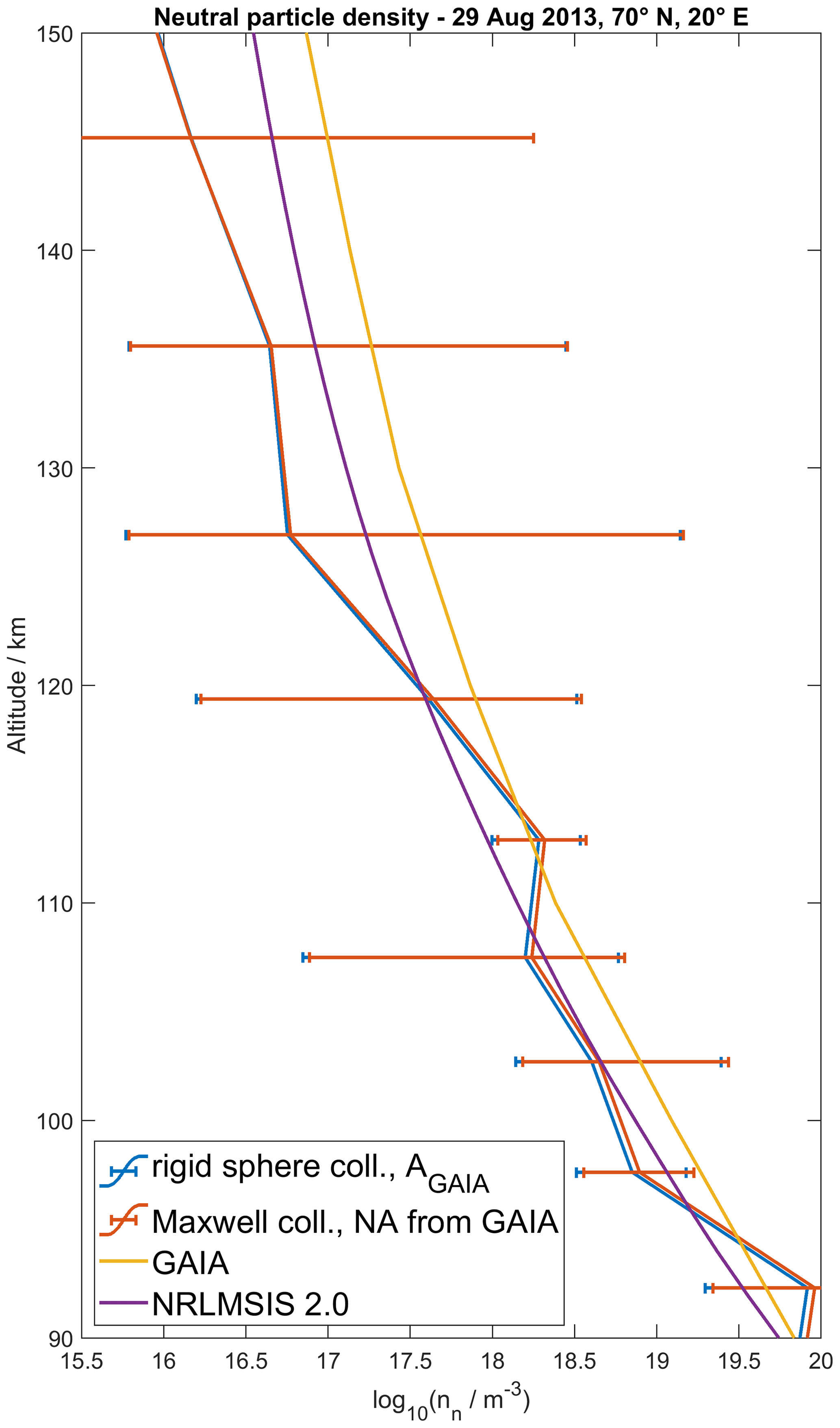
Figure 6Neutral density profiles calculated from the measured ion–neutral collision frequencies for either rigid-sphere or Maxwell collisions. For both methods, the mean neutral mass and the abundances of the different neutral species (NA) have been taken from GAIA. For comparison, profiles from the NRLMSIS 2.0 and GAIA models are shown.
The variability of the measured neutral density profile nn,mes can be seen from the relative variation . For a better comparison with Nicolls et al. (2014), we calculate the relative variation of neutral mass density . Since the atmospheric composition has to be assumed for the calculation of neutral particles already, this step does not require any additional assumptions.
Figure 7 shows the relative variation of measured neutral mass density compared to the NRLMSIS 2.0 model. It can be seen that the neutral mass density measurements oscillate around the MSIS climatology below 120 km altitude with a relative amplitude of ∼0.5–1. The obtained profile renders previously presented results (Fig. 5 in Nicolls et al., 2014). Deviations of the vertical profile from the climatological background were interpreted as tidal or lower-frequency oscillations.
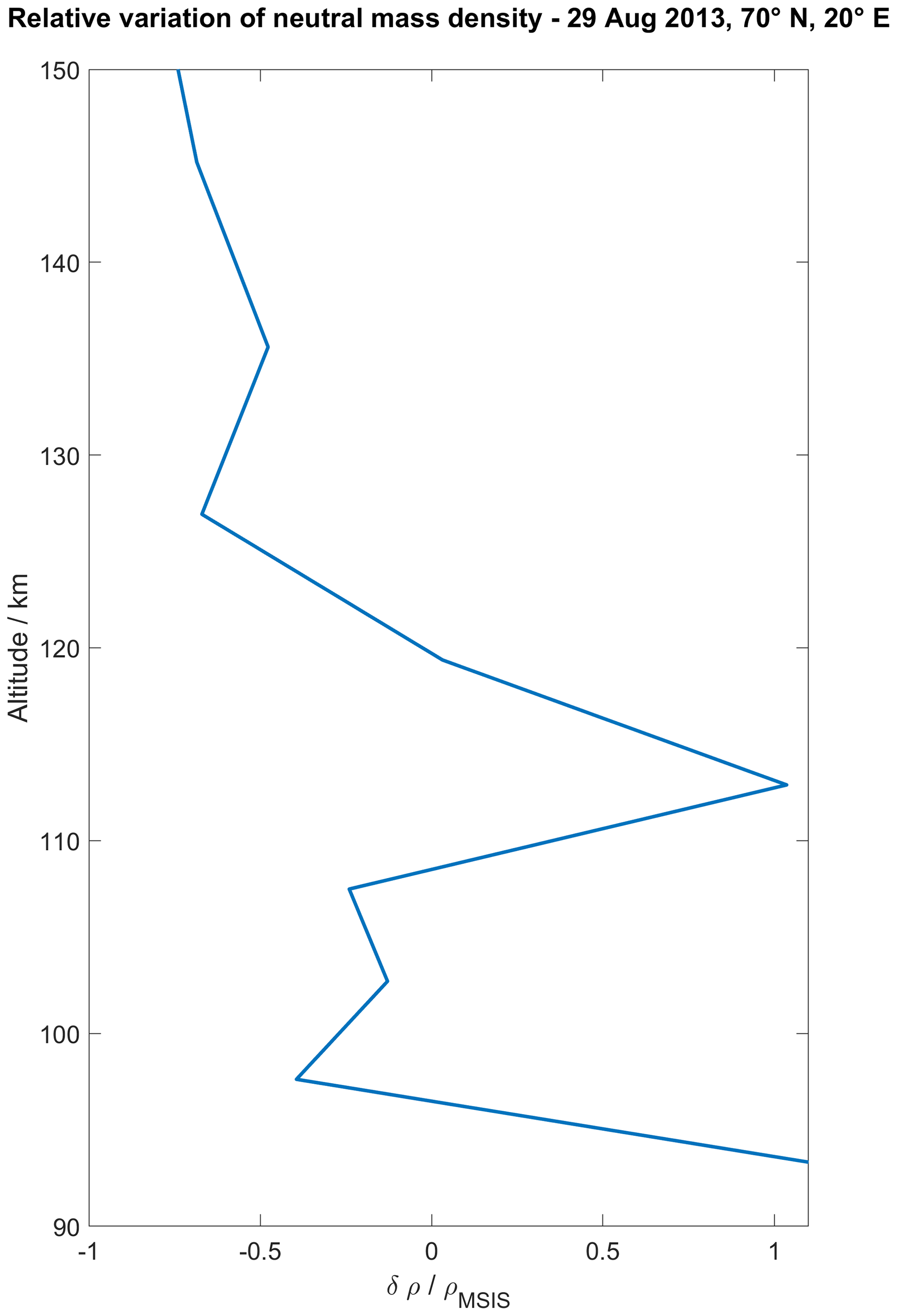
Figure 7Variation of the neutral mass density calculated from the measured ion–neutral collision frequency profile relative to the NRLMSIS 2.0 mass density.
Since there have been no previous experimental studies applying the difference spectrum method, the obtained results can only be compared to multifrequency measurements applying a different analysis method and both direct and indirect measurements of the ion–neutral collision frequency. The νin profiles in Fig. 3 can be compared to the results by Nicolls et al. (2014), since they were obtained from the same measurements. The profile obtained for the β parameter determined at hβ=150 km altitude agrees well with the results obtained in Nicolls et al. (2014). As shown in Fig. 4, the β parameter is altitude dependent for the EISCAT campaign on 29 August 2013, though it is expected to be roughly constant for all altitudes where νin≈0 can be assumed (Grassmann, 1993b). The β profile for the EISCAT measurements from 27 September 2021 shows a distinctly lower rate of change with altitude. Since there are more than 8 years between the two measurements, technical updates of the system might explain the different behavior of the parameter. Since the beam shapes of the UHF and the VHF system are not identical, the scatter volumes are close but also not identical. Therefore, already minor system updates or degradations of one of the systems can significantly impact the result of our dual-frequency analysis, which is performed under the assumption of identical scatter volumes. The decrease in β with altitude indicates that the amplitude of the UHF spectrum decreases more strongly with altitude than the amplitude of the VHF spectrum.
The νin profile obtained for 27 September 2021, shown in Fig. 2, shows an increased collision frequency above 115 km altitude compared to the climatology. This agrees with previous findings (Fig. 2 in Nygrén, 1996), which show an increase in νin compared to the MSIS-86 climatology above 110 km for a single campaign on 26 August 1985. Nygrén (1996) combined both the direct measurement of νin from the ISR spectrum, assuming Te=Ti, and the indirect measurement from vertical ion drifts. Oyama et al. (2012) also reported an increased collision frequency above about 120 km during ionospheric heating events at E-region altitudes. They interpreted this as the result of an upward motion of denser neutral gas from lower altitudes. In Fig. 2, the minimum of νin around 105 km altitude, in combination with the very slow decrease above, could be explained by thermospheric gas being transported upward from the altitude of the minimum.
Ion–neutral collision frequency measurements are of special interest for atmospheric physics, since they allow us to infer information about neutral gas densities in the MLT region. There are multiple methods to calculate collision frequencies from neutral particle densities, two of which are presented in Fig. 6 for the EISCAT measurements on 29 August 2013. One method assumes both ions and neutrals to be rigid spheres, while the other assumes Maxwell collision between the ions and the polarized neutrals. While the rigid-sphere collision model only requires assumptions on the mean neutral particle mass, the abundances of the different neutral particle sorts have to be assumed for the Maxwell collision model. Figure 6 shows that the choice of collision model has a far greater impact on the neutral density profile than the assumptions about mean neutral mass or particle abundances. Comparison to one empirical atmosphere model (NRLMSIS 2.0) and one physics-based model (GAIA) resulted in expectable agreement and disagreement. Both models display a smooth neutral density profile and do not capture small-scale dynamics but, on the other hand, indicate the expected vertical behavior. For validation of our measurements, a gravity-wave-resolving model, which includes incompressibility terms for small scales such as the High Altitude Mechanistic general Circulation Model (HIAMCM) (Becker and Vadas, 2020), would be required. In future studies, the inferred neutral density profiles could also be validated by comparison to meteor radar measurements. The neutral particle density can be obtained from meteor radar measurements, with the meteor peak flux altitude as a proxy (Stober et al., 2012). Figure 7 was designed following the example of Fig. 5 in Nicolls et al. (2014), and they agree reasonably well. The relative variation of the neutral mass density shows periodic oscillations, which were interpreted as the result of tides and lower-frequency oscillations by Nicolls et al. (2014).
Additionally, there are possible improvements to the general analysis of ISR measurements, applicable for all described collision frequency measurements, including the one presented in this paper. One possible improvement for all discussed analysis techniques could be the application of full profile analysis (Lehtinen et al., 1996). Instead of analyzing each altitude gate independently, as is done in this study and Nicolls et al. (2014), the total vertical profile of the plasma parameters could be fitted during full profile analysis. The assumption that the plasma parameters are constant within each altitude gate is, therefore, not required for full profile analysis (Lehtinen et al., 1996).
In this paper, we presented the first application of the difference spectrum method to analyze multifrequency ISR measurements to obtain direct measurements of the ion–neutral collision frequency. We showed that this method can be applied in combination with standard ISR analysis software (GUISDAP). Comparison to the only previous multifrequency ISR measurement, which applied special software to analyze two ISR measurements simultaneously, showed reasonable agreement. Therefore the difference spectrum method can be applied as an equivalent multifrequency ISR analysis method, generally applicable without the requirement of highly specialized ISR analysis software. This is the main advantage of the method presented here over other multifrequency methods. Multifrequency methods are generally advantageous for collision frequency measurements, since they do not require additional assumptions like Te=Ti or strong electric fields.
We presented ion–neutral collision frequency profiles from three different EISCAT multifrequency campaigns. The measurements from 29 August 2013 were applied for comparison to the other multifrequency analysis method. Contrary to our expectation, the scaling parameter β was not constant at nearly collisionless altitudes, which could indicate a problem with one of the systems at the time. The second multifrequency campaign that we analyzed was conducted on 27 September 2021 in the same radar mode as the previous campaign. The vertical β parameter profile exhibited a significantly lower gradient in the F region for these measurements. At about 100–115 km altitude, the measurements showed a notably lower collision frequency than the climatology, while the collision frequency was larger than the climatology above 115 km. This might be the result of an upward motion of neutral gas due to ionospheric heating, e.g., caused by Joule dissipation. The third analyzed multifrequency campaign was conducted on 13 October 2022 and applied a different radar mode than the previous ones. The EISCAT manda radar mode allows measurements in the lower thermosphere with a very high altitude resolution, which might be helpful to study phenomena with a small-scale altitude structure.
In general, further improvement of the difference spectrum method, as well as multifrequency experiments, is required. Possible improvements would be the already mentioned application of full profile analysis of the ion–neutral collision frequency or the general improvement of ISR fitting by including the exact ion chemistry of the ionosphere. Validation of our collision frequency and neutral density measurements is difficult due to the general lack of observational methods in the ionospheric transition region. However, the manda measurements cover and resolve a good part of the meteor radar altitudes at about 80–110 km. Meteor radar neutral density measurements could be one possibility to verify multifrequency ISR experiments. As shown in Sect. 4, the comparison to neutral atmosphere models is only somewhat meaningful, as long as the models do not include the incompressibility terms for small-scale variability, e.g., due to gravity waves. Considering the lack of atmospheric measurement methods in the ionospheric dynamo region, the method presented here is highly valuable because it provides information about this important region.
The data are available under the Creative Commons Attribution 4.0 International license at https://doi.org/10.5281/zenodo.8074787 (Günzkofer et al., 2023).
FG performed the data analysis and wrote large parts of the manuscript. DP suggested the idea to analyze multifrequency experiments. All authors provided feedback and were involved in revising the manuscript.
The contact author has declared that none of the authors has any competing interests.
Publisher's note: Copernicus Publications remains neutral with regard to jurisdictional claims made in the text, published maps, institutional affiliations, or any other geographical representation in this paper. While Copernicus Publications makes every effort to include appropriate place names, the final responsibility lies with the authors.
EISCAT is an international association supported by research organizations in China (CRIRP), Finland (SA), Japan (NIPR and ISEE), Norway (NFR), Sweden (VR), and the United Kingdom (UKRI). The dataset used for this study is from the Ground-to-topside model of the Atmosphere and Ionosphere for Aeronomy (GAIA) project carried out by the National Institute of Information and Communications Technology (NICT), Kyushu University, and Seikei University. Gunter Stober is a member of the Oeschger Center for Climate Change Research (OCCR).
The article processing charges for this open-access publication were covered by the German Aerospace Center (DLR).
This paper was edited by Wen Yi and reviewed by three anonymous referees.
Baumjohann, W. and Treumann, R. A.: Basic space plasma physics, World Scientific, https://doi.org/10.1142/p015, 1996. a
Becker, E. and Vadas, S. L.: Explicit Global Simulation of Gravity Waves in the Thermosphere, J. Geophys. Res.-Space, 125, e28034, https://doi.org/10.1029/2020JA028034, 2020. a
Brekke, A., Doupnik, J. R., and Banks, P. M.: A preliminary study of the neutral wind in the auroral E region, J. Geophys. Res., 78, 8235–8250, https://doi.org/10.1029/JA078i034p08235, 1973. a
Brekke, A., Doupnik, J. R., and Banks, P.: Incoherent scatter measurements of E region conductivities and currents in the auroral zone, J. Geophys. Res., 79, 3773–3790, https://doi.org/10.1029/JA079i025p03773, 1974. a
Chapman, S.: The electrical conductivity of the ionosphere: A review, Il Nuovo Cimento, 4, 1385–1412, https://doi.org/10.1007/BF02746310, 1956. a, b, c
Dalgarno, A., McDowell, M. R. C., and Williams, A.: The Mobilities of Ions in Unlike Gases, Philos. T. Roy. Soc. A, 250, 411–425, https://doi.org/10.1098/rsta.1958.0002, 1958. a
Dawkins, E. C. M., Stober, G., Janches, D., Carrillo-Sánchez, J. D., Lieberman, R. S., Jacobi, C., Moffat-Griffin, T., Mitchell, N. J., Cobbett, N., Batista, P. P., Andrioli, V. F., Buriti, R. A., Murphy, D. J., Kero, J., Gulbrandsen, N., Tsutsumi, M., Kozlovsky, A., Kim, J. H., Lee, C., and Lester, M.: Solar Cycle and Long-Term Trends in the Observed Peak of the Meteor Altitude Distributions by Meteor Radars, Geophys. Res. Lett., 50, e2022GL101953, https://doi.org/10.1029/2022GL101953, 2023. a
Dougherty, J. P. and Farley, D. T., J.: A Theory of Incoherent Scattering of Radio Waves by a Plasma, 3 Scattering in a Partly Ionized Gas, J. Geophys. Res.-Space, 68, 5473, https://doi.org/10.1029/JZ068i019p05473, 1963. a
Emmert, J. T., Drob, D. P., Picone, J. M., Siskind, D. E., Jones, M., Mlynczak, M. G., Bernath, P. F., Chu, X., Doornbos, E., Funke, B., Goncharenko, L. P., Hervig, M. E., Schwartz, M. J., Sheese, P. E., Vargas, F., Williams, B. P., and Yuan, T.: NRLMSIS 2.0: A Whole Atmosphere Empirical Model of Temperature and Neutral Species Densities, Astr. Soc. P., 8, e01321, https://doi.org/10.1029/2020EA001321, 2021. a
Farley, D. T.: A theory of incoherent scattering of radio waves by a plasma: 4. The effect of unequal ion and electron temperatures, J. Geophys. Res.-Space, 71, 4091–4098, https://doi.org/10.1029/JZ071i017p04091, 1966. a
Folkestad, K., Hagfors, T., and Westerlund, S.: EISCAT: An updated description of technical characteristics and operational capabilities, Radio Sci., 18, 867–879, https://doi.org/10.1029/RS018i006p00867, 1983. a
Grassmann, V.: The effect of different collision operators on EISCAT's standard data analysis model, J. Atmos. Terr. Phys., 55, 567–571, https://doi.org/10.1016/0021-9169(93)90005-J, 1993a. a
Grassmann, V.: An incoherent scatter experiment for the measurement of particle collisions, J. Atmos. Terr. Phys., 55, 573–576, https://doi.org/10.1016/0021-9169(93)90006-K, 1993b. a, b, c, d, e, f, g, h, i
Günzkofer, F., Pokhotelov, D., Stober, G., Liu, H., Liu, H. L., Mitchell, N. J., Tjulin, A., and Borries, C.: Determining the Origin of Tidal Oscillations in the Ionospheric Transition Region With EISCAT Radar and Global Simulation Data, J. Geophys. Res.-Space, 127, e2022JA030861, https://doi.org/10.1029/2022JA030861, 2022. a, b
Günzkofer, F., Stober, G., Pokhotelov, D., Miyoshi, Y., and Borries, C.: [Dataset] Difference spectrum fitting of the ion-neutral collision frequency from dual-frequency EISCAT measurements, Zenodo [data set], https://doi.org/10.5281/zenodo.8074787, 2023. a
Hedin, A. E.: Extension of the MSIS thermosphere model into the middle and lower atmosphere, J. Geophys. Res.-Space, 96, 1159–1172, https://doi.org/10.1029/90JA02125, 1991. a
Jin, H., Miyoshi, Y., Pancheva, D., Mukhtarov, P., Fujiwara, H., and Shinagawa, H.: Response of migrating tides to the stratospheric sudden warming in 2009 and their effects on the ionosphere studied by a whole atmosphere-ionosphere model GAIA with COSMIC and TIMED/SABER observations, J. Geophys. Res.-Space, 117, A10323, https://doi.org/10.1029/2012JA017650, 2012. a
Katsuda, S., Enoto, T., Lommen, A. N., Mori, K., Motizuki, Y., Nakajima, M., Ruhl, N. C., Sato, K., Stober, G., Tashiro, M. S., Terada, Y., and Wood, K. S.: Long-Term Density Trend in the Mesosphere and Lower Thermosphere From Occultations of the Crab Nebula With X-Ray Astronomy Satellites, J. Geophys. Res.-Space, 128, e2022JA030797, https://doi.org/10.1029/2022JA030797, 2023. a
Kelly, M. C.: The Earth's Ionosphere: Plasma Physics and Electrodynamics, Second Edition, Elsevier Academic Press, ISBN 978-0-12-088425-4, 2009. a
Kobayashi, S., Ota, Y., Harada, Y., Ebita, A., Moriya, M., Onoda, H., Onogi, K., Kamahori, H., Kobayashi, C., Endo, H., Miyaoka, K., and Takahashi, K.: The JRA-55 Reanalysis: General Specifications and Basic Characteristics, J. Meteorol. Soc. Jpn., 93, 5–48, https://doi.org/10.2151/jmsj.2015-001, 2015. a
Lehtinen, M. S. and Huuskonen, A.: General incoherent scatter analysis and GUISDAP, J. Atmos. Terr. Phys., 58, 435–452, https://doi.org/10.1016/0021-9169(95)00047-X, 1996. a
Lehtinen, M. S., Huuskonen, A., and Pirttilä, J.: First experiences of full-profile analysis with GUISDAP, Ann. Geophys., 14, 1487–1495, https://doi.org/10.1007/s00585-996-1487-3, 1996. a, b
Nicolet, M.: The collision frequency of electrons in the ionosphere, J. Atmos. Terr. Phys., 3, 200–211, https://doi.org/10.1016/0021-9169(53)90110-X, 1953. a, b
Nicolls, M. J., Bahcivan, H., Häggström, I., and Rietveld, M.: Direct measurement of lower thermospheric neutral density using multifrequency incoherent scattering, Geophys. Res. Lett., 41, 8147–8154, https://doi.org/10.1002/2014GL062204, 2014. a, b, c, d, e, f, g, h, i, j, k, l, m
Nozawa, S., Ogawa, Y., Oyama, S., Fujiwara, H., Tsuda, T., Brekke, A., Hall, C. M., Murayama, Y., Kawamura, S., Miyaoka, H., and Fujii, R.: Tidal waves in the polar lower thermosphere observed using the EISCAT long run data set obtained in September 2005, J. Geophys. Res.-Space, 115, A08312, https://doi.org/10.1029/2009JA015237, 2010. a, b, c
Nygrén, T.: Studies of the E-region ion-neutral collision frequency using the EISCAT incoherent scatter radar, Adv. Space Res., 18, 79–82, https://doi.org/10.1016/0273-1177(95)00843-4, 1996. a, b, c
Nygren, T., Jalonen, L., and Huuskonen, A.: A new method of measuring the ion-neutral collision frequency using incoherent scatter radar, Planet. Space Sci., 35, 337–343, https://doi.org/10.1016/0032-0633(87)90160-7, 1987. a
Oyama, S., Kurihara, J., Watkins, B. J., Tsuda, T. T., and Takahashi, T.: Temporal variations of the ion-neutral collision frequency from EISCAT observations in the polar lower ionosphere during periods of geomagnetic disturbances, J. Geophys. Res.-Space, 117, A05308, https://doi.org/10.1029/2011JA017159, 2012. a, b
Picone, J. M., Hedin, A. E., Drob, D. P., and Aikin, A. C.: NRLMSISE-00 empirical model of the atmosphere: Statistical comparisons and scientific issues, J. Geophys. Res.-Space, 107, 1468, https://doi.org/10.1029/2002JA009430, 2002. a, b
Schunk, R. and Nagy, A.: Ionospheres: Physics, Plasma Physics, and Chemistry, edited by: Houghton, J. T., Rycroft, M. J., and Dessler, A. J., Cambridge University Press, https://doi.org/10.1017/CBO9780511635342, 2009. a, b, c
Stober, G., Jacobi, C., Matthias, V., Hoffmann, P., and Gerding, M.: Neutral air density variations during strong planetary wave activity in the mesopause region derived from meteor radar observations, J. Atmos. Sol.-Terr. Phy., 74, 55–63, https://doi.org/10.1016/j.jastp.2011.10.007, 2012. a, b
Stober, G., Matthias, V., Brown, P., and Chau, J. L.: Neutral density variation from specular meteor echo observations spanning one solar cycle, Geophys. Res. Lett., 41, 6919–6925, https://doi.org/10.1002/2014GL061273, 2014. a
Stober, G., Kuchar, A., Pokhotelov, D., Liu, H., Liu, H.-L., Schmidt, H., Jacobi, C., Baumgarten, K., Brown, P., Janches, D., Murphy, D., Kozlovsky, A., Lester, M., Belova, E., Kero, J., and Mitchell, N.: Interhemispheric differences of mesosphere–lower thermosphere winds and tides investigated from three whole-atmosphere models and meteor radar observations, Atmos. Chem. Phys., 21, 13855–13902, https://doi.org/10.5194/acp-21-13855-2021, 2021. a
Stober, G., Weryk, R., Janches, D., Dawkins, E. C., Günzkofer, F., Hormaechea, J. L., and Pokhotelov, D.: Polarization dependency of transverse scattering and collisional coupling to the ambient atmosphere from meteor trails – theory and observations, Planet. Space Sci., 237, 105768, https://doi.org/10.1016/j.pss.2023.105768, 2023. a
Tjulin, A.: EISCAT experiments, Tech. rep., EISCAT Scientific Association, https://eiscat.se/wp-content/uploads/2021/03/Experiments_v20210302.pdf (last access: 6 December 2023), 2021. a
- Abstract
- Introduction
- Instruments and models
- Difference spectrum fitting of the ion–neutral collision frequency
- Neutral density measurements and comparison to atmospheric models
- Discussion
- Conclusions
- Data availability
- Author contributions
- Competing interests
- Disclaimer
- Acknowledgements
- Financial support
- Review statement
- References