Results of a long-term international comparison of greenhouse gas and isotope measurements at the Global Atmosphere Watch (GAW) Observatory in Alert, Nunavut, Canada

Since 1999, Environment and Climate Change Canada (ECCC) has been coordinating a multi-laboratory comparison of measurements of long-lived greenhouse gases in whole air samples collected at the Global Atmosphere Watch (GAW) Alert Observatory located in the Canadian High Arctic (82^∘28^′ N, 62^∘30^′ W). In this paper, we evaluate the measurement agreement of atmospheric CO₂, CH₄, N₂O, SF₆, and stable isotopes of CO₂ (δ¹³C, δ¹⁸O) between leading laboratories from seven independent international institutions. The measure of success is linked to target goals for network compatibility outlined by the World Meteorological Organization's (WMO) GAW greenhouse gas measurement community. Overall, based on ∼ 8000 discrete flask samples, we find that the co-located atmospheric CO₂ and CH₄ measurement records from Alert by CSIRO, MPI-BGC, SIO, UHEI-IUP, and ECCC versus NOAA (the designated reference laboratory) are generally consistent with the WMO compatibility goals of ± 0.1 ppm CO₂ and ± 2 ppb CH₄ over the 17-year period (1999–2016), although there are periods where differences exceed target levels and persist as systematic bias for months or years. Consistency with the WMO goals for N₂O, SF₆, and stable isotopes of CO₂ (δ¹³C, δ¹⁸O) has not been demonstrated. Additional analysis of co-located comparison measurements between CSIRO and SIO versus NOAA or INSTAAR (for the isotopes of CO₂) at other geographical sites suggests that the findings at Alert for CO₂, CH₄, N₂O, and δ¹³C–CO₂ could be extended across the CSIRO, SIO, and NOAA observing networks. The primary approach to estimate an overall measurement agreement level was carried out by pooling the differences of all individual laboratories versus the designated reference laboratory and determining the 95th percentile range of these data points. Using this approach over the entire data record, our best estimate of the measurement agreement range is −0.51 to +0.53 ppm for CO₂, −0.09 ‰ to +0.07 ‰ for δ¹³C, −0.50 ‰ to +0.58 ‰ for δ¹⁸O, −4.86 to +6.16 ppb for CH₄, −0.75 to +1.20 ppb for N₂O, and −0.14 to +0.09 ppt for SF₆. A secondary approach of using the average of 2 standard deviations of the means for all flask samples taken in each individual sampling episode provided similar results. These upper and lower limits represent our best estimate of the measurement agreement at the 95 % confidence level for these individual laboratories, providing more confidence for using these datasets in various scientific applications (e.g., long-term trend analysis).

1 Introduction

For more than 60 years, scientists have been making high-precision measurements of atmospheric CO₂ (Keeling, 1960). At first, the objective was to understand global features in well-mixed marine air by documenting CO₂ abundance, seasonal patterns, and trends. For this purpose, only a few remote sampling sites were established. Over time the emphasis has shifted to better understand the carbon cycle including emissions to and removal processes from the atmosphere. Today, a global observational network maintained by many laboratories operates high-precision measurements of long-lived greenhouse gases (GHGs) and complementary trace species at hundreds of locations (WMO, 2019, 2022). The measurement community has held regular meetings on measurement technology since 1975, initiated by Charles David Keeling. These meetings are known as “carbon dioxide, other greenhouse gases, and related measurement techniques (GGMT) meetings” and are sponsored by the WMO and International Atomic Energy Agency (IAEA). Proceedings from these meetings are published in Global Atmosphere Watch (GAW) reports (e.g., GAW Report, 2016, 2018, 2020), which are important references for existing and new laboratories. These reports include measurement target recommendations for GHG network compatibility. These targets reflect the scientifically desirable level of network agreement in measurements of well-mixed background air, so the data of different laboratories can be used together in global models or to infer regional GHG fluxes.

Atmospheric measurements of CO₂ and other trace gas species and isotopes are reported by many international laboratories and are often freely available either directly from the originating measurement laboratory (Masarie and Tans, 1995; Masarie et al., 2014; Ramonet et al., 2020; Heimann et al., 2022) or from the WMO World Data Centre for Greenhouse Gases (WDCGG) (https://gaw.kishou.go.jp, last access: 17 November 2023). For nearly 30 years, atmospheric measurements of CO₂ have been used to derive estimates of CO₂ surface fluxes around the globe (Heimann and Keeling, 1989; Tans et al., 1990; Fan et al., 1998; Bousquet et al., 2000; Gloor et al., 2000; Gurney et al., 2002; Peters et al., 2007; Chevallier et al., 2010; Peylin et al., 2013; Rödenbeck et al, 2018a, b; Friedlingstein et al., 2022). Similar studies have also been carried out for CH₄ (Houweling et al., 2017) and N₂O (Schilt et al., 2010; Thompson et al., 2019). When all available datasets are used in those applications, the users usually assume that these datasets are compatible and consistent over time. However, the applications may be limited by various types of inconsistencies between the datasets, including differences in scales or scale realizations and in sampling systems or procedures, etc. When persistent bias exists between laboratories, the applications such as flux estimates derived by modeling systems using combined datasets on various spatial domains and temporal scales can have large uncertainties (Masarie et al., 2001; Ramonet et al., 2020). To address potential bias, laboratories routinely evaluate measurement traceability and reproducibility within their own laboratory and also compare their measurements with those from other laboratories. Data providers in the measurement community are working hard to include uncertainties with their measurements in order to inform data users. For these reasons, evaluating and quantifying the inconsistencies, biases, or level of agreements for observational records within and between laboratories over time is important.

The widely adopted strategy for assessing the level of agreement of different atmospheric trace gas data records is to conduct ongoing comparisons of the measurements of flask air collected at the same time and the same location (Masarie et al., 2001, 2003; Langenfelds et al., 2003). Based on these previous studies, which involved the comparison of only two laboratories at the same location, this comparison strategy can reveal differences from air sample collection, storage, extraction and analysis, data processing, and maintenance of the laboratory calibration scale, etc. Subtle problems can arise at any step in the measurement procedure. They can occur simultaneously and may exist in one or more of the participating laboratories. Identifying the cause(s) of these inconsistencies often proves difficult (Masarie et al., 2001). Many laboratories often participate in additional comparison experiments designed to help elucidate the cause(s) of observed differences. Laboratories also realize that when comparison results are examined in near-real time, the information can be a valuable quality control measure where problems can potentially be detected and addressed soon after they develop (Levin et al., 2020). A data comparison site administered by NOAA and accessible exclusively to data providers was established for ongoing comparisons in 1999, and it is still in operation today. This platform provides preliminary comparisons for quality control purposes and serves as a good starting point for further in-depth analysis.

The Alert Observatory (ALT), Canada, along with the Mauna Loa Observatory (MLO), USA, and the Cape Grim Observatory (CGO), Australia, are designated as GHG comparison sites by WMO-GAW (GAW Report, 2006), where well-mixed background air can be sampled and measured. Alert has the most extensive flask comparison program of the three with seven individual flask programs at any time, each focusing on a variety of measurements and respective scientific priorities. In addition, the corresponding comparison results among the three sites (ALT, MLO, and CGO) can provide more information on site-specific inconsistencies and facilitate merging the data records from individual networks.

In this paper, we present the comparison results of atmospheric CO₂, CH₄, N₂O, and SF₆ and the stable isotopes of CO₂ (δ¹³C, δ¹⁸O) measured by the seven international institutions at Alert over the period of 1999–2016. Although some laboratories have measurements prior to 1999 and continue after 2016, this period was chosen because it includes the largest number of laboratories and species measured. The participating institutions are Environment and Climate Change Canada (ECCC), Commonwealth Scientific and Industrial Research Organisation (CSIRO), Max Planck Institute for Biogeochemistry (MPI-BGC), Heidelberg University, Institut für Umweltphysik (UHEI-IUP), Laboratoire des Sciences du Climat et de l'Environnement (LSCE), Scripps Institution of Oceanography (SIO), and the National Oceanic and Atmospheric Administration (NOAA) in collaboration with the Stable Isotope Laboratory at the University of Colorado Institute of Arctic and Alpine Research (INSTAAR). Together with Alert results, we also present corresponding comparisons between CSIRO, SIO, and NOAA at MLO and between CSIRO and NOAA at CGO for the same time period (1999–2016). This is the first report of such a large-scale comparison study. While timely publications of the inter-comparison results are desirable, it can be challenging due to the large number of groups involved and ongoing evolving parameters including the adoption of new calibration scales, data corrections, and the limited dedicated resources to carry out these exercises.

2 Methods

2.1 Types of comparison

The commonly used measurement approaches for GHGs and related tracers include (1) discrete flask air samples collected in the field (commonly collected as a pair or as multiple flasks in series or in parallel) and shipped to a measurement laboratory or laboratories for analysis and (2) continuous measurements in situ, conducted using analytical equipment located at the sampling location. The two approaches are complementary, and each approach will remain essential due to their respective advantages and disadvantages. In situ measurements can provide information at very high temporal resolution so that synoptic-scale meteorological events can be observed, which may only by chance be captured by a weekly discrete air sample. In situ monitoring approach requires a physical facility with reliable power, easy access as well as a high degree of automation, and internet capability to monitor the observation systems remotely. On the other hand, flask air samples are returned to the laboratories with sufficient air, and many laboratories can measure multiple trace gases and their stable isotopes from a single discrete air sample. Also, the relatively low operating cost and minimal infrastructure requirements of flask sampling allows for spatial coverage involving more locations. Many laboratories have opted for an approach including discrete flask-air sampling and, when possible, in situ measurements at one or two key sites to balance temporal and spatial coverage and a suite of measured species.

This study presents two types of discrete flask comparisons, which are known as co-located and same-flask comparisons. The focus is the co-located comparisons, but results from the same-air flask comparisons, as well as same-cylinder (round robins) comparisons, are included to help facilitate the interpretation of the co-located comparison results. These complementary comparisons could reveal cumulative differences due to errors introduced at one or more steps in the entire sampling and measurement process.

Co-located flask air measurement comparison. A co-located comparison generally describes a comparison of two or more measurement records derived using independent collection systems or methods and/or analytical systems at the same location, at approximately the same time and during predefined atmospheric conditions (i.e., wind direction and minimum wind speed requirements). When these conditions are met, observed differences are primarily due to experimental discrepancies instead of changes in the atmospheric signal. Co-located comparisons are designed to evaluate the measurement agreements within or between laboratories due to uncertainties associated with sampling procedures/systems, analytical procedures, data processing, and laboratory calibration scales. Potential errors could arise from any or all of the steps.

Same-flask air measurement comparison. A same-flask air comparison evaluates the independent measurement results when two or more programs or analytical systems measure air from the same “collected sample” container for the same suite of trace species. Typically, the same-flask air comparison sample is shipped from the remote sampling location to the closest participating laboratory or to the laboratory with lowest sample consumption. This same-flask sample is then shipped to a second participating laboratory for analysis. Additional laboratories or analytical systems could further analyze the sample, provided there is sufficient air remaining in the flask, although the risk of sample contamination or alteration may increase. A same-flask comparison experiment evaluates the measurement agreement within or between laboratories caused only by measurement and data processing steps and not by sample collection procedures/systems. A problem during sample collection, such as contamination, could still potentially affect the air in the flask, but this should not impact the comparison results for same-flask analysis. Typically, only one flask of a pair is analyzed by both labs, thereby providing information whether the analysis procedure by one of the labs has caused contamination or altered the composition of the air in the flask. The reference laboratory for same-flask comparisons at Alert is ECCC.

Same-cylinder air measurement comparison. A same-cylinder air measurement comparison refers to an experiment in which two or more laboratories measure air in a pressurized cylinder for the same suite of trace species and then compare the independent measurement results. Like the same-flask air comparison experiment, the same-cylinder air comparison evaluates the measurement agreements within or between laboratories involving the overall uncertainties from analytical procedures (i.e., extracting air from the cylinder, introducing the aliquot of air into their detection system, measuring the sample) to processing the results and maintaining their laboratory calibration scales. Because the volume of air sample in a pressurized cylinder is orders of magnitude greater than that in a flask, many more laboratories can participate in the comparison, and each laboratory can make multiple measurements thereby obtaining an optimized measurement uncertainty. One drawback of the same-cylinder comparison is the added time and expense of shipping pressurized cylinders, which can be subject to strict international safety regulations. Consequently, the frequency for this type of comparison is from quarterly, at best, to every few years and the results only represent a snapshot in time. It should be noted that analyzers used to measure flask samples are not necessarily the same instruments that are used for cylinder air analysis in each laboratory, and this can contribute uncertainty and possibly bias to the comparison. It is important in these types of comparisons that at least one laboratory, generally the coordinating laboratory, measures the air before and after any other laboratories to characterize/quantify any composition changes that may have occurred during the period of comparison. In addition, it is important to note that drifts in concentrations may occur with cylinder depressurization.

The WMO/IAEA “Round Robin” (RR) Comparison Experiment, administered by NOAA, is one example of a same-cylinder air comparison experiment. This experiment is designed to assess the level of agreement within the participating laboratories and assess their ability to maintain links to the WMO mole fraction scales for CO₂, CH₄, and other trace gas species. There have been seven WMO/IAEA Round Robin experiments since it was first introduced in 1974; the most recent experiment started in November of 2020, includes participation by 59 laboratories (Global Monitoring Laboratory – Carbon Cycle Greenhouse Gases (https://gml.noaa.gov/ccgg/wmorr/, last access: 17 November 2023)), and is still ongoing. Round robin results from RR nos. 5 and 6 from the participating laboratories are included in certain figures and in Table S1 in the Supplement, if the results are on the same scale as the data used in this analysis.

2.2 The Alert Dr. Neil Trivett Global Atmosphere Watch Observatory

Alert, Nunavut, is located on the northern tip of Ellesmere Island in the Canadian High Arctic (82^∘28^′ N, 62^∘30^′ W) far from the major industrial regions of the Northern Hemisphere. Alert is the site of a military station, Canadian Forces Station (CFS) Alert, and an ECCC Upper Air Weather Station. The Alert Dr. Neil Trivett Global Atmosphere Watch (GAW) Observatory (ALT) is located 6 km south of CFS Alert on a plateau 210 m above sea level. The land around Alert is covered with snow for almost 10 months of the year and has a sparse covering of polar desert vegetation in the summer. The degree of contamination from the local environment is minimal, with winds originating from within the ENE sector, which includes CFS Alert camp (Worthy et al., 1994), less than 4 % of the time. The ALT observatory is ideally situated for monitoring well-mixed air masses representative of very large spatial extent in the Northern Hemisphere. ALT has been the cornerstone of ECCC's atmospheric research program since 1975, and in 1986 it was officially designated a WMO-GAW Global Observatory. The observatory was officially renamed the Dr. Neil Trivett Global Atmosphere Watch Observatory in 2006. With its existing infrastructure and strong multi-laboratory research activity, ALT is well positioned to support a multi-laboratory co-located atmospheric comparison experiment.

2.3 Flask sampling at ALT, MLO, and CGO

2.3.1 Sampling timelines

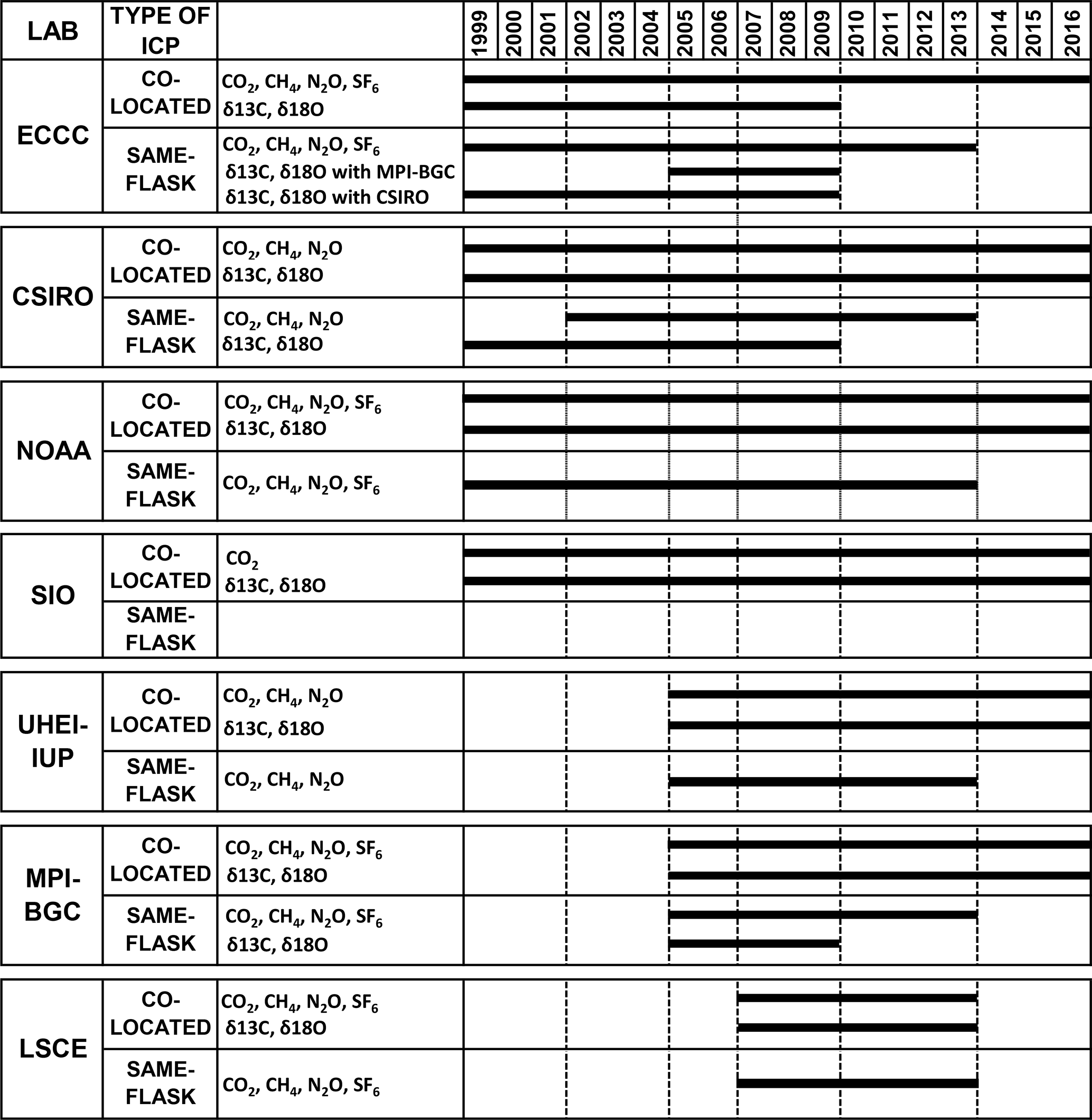
The species measured, types of comparisons (co-located/same flask), and timelines of comparison experiments conducted at Alert from 1999–2016 are summarized in Table 1. Individual laboratory participation and species measured were not consistent over the entire 17-year period. For example, ECCC's program for CO₂ isotopes was terminated in December 2009, and LSCE's program for all trace gases and isotopes was discontinued in September 2013. The same flask air comparison program for all trace gases at Alert has an end date of December 2013.

At MLO and CGO, co-located flask sampling was conducted by CSIRO, SIO, and NOAA for the same species and similar time periods as  ALT.

Table 1 Summary of available observations and flask comparison types for each participating laboratory during the period of this study at ALT.

2.3.2 Sampling systems

Table 2a describes the sample collection system at ALT for each laboratory, including flask type, sampling frequency, and apparatus used during the specified time period. Most laboratories at ALT used double-stopcock flasks, which allow for flow-through flushing prior to filling to an overpressure of 5 to 15 psi. Exceptions include SIO, who used single-stopcock and evacuated flasks, and CSIRO, who used some single-stopcock pressurized flasks from 1999 to 2003. Air was typically dried using a cryocooler before filling by most laboratories, except SIO and NOAA, who did not dry their air samples either by a cryocooler or by a chemical dryer, and MPI-BGC, who used a Mg(ClO₄)₂ dryer until 2015 before switching to a cryocooler. Sampling was conducted at a height of 10 m, except SIO and NOAA, whose intakes were roughly 2 and 5 m, respectively.

At MLO, SIO's sampling was the same as ALT, but CSIRO's sampling used a chemical dryer instead of a cryocooler and had a 40 m air intake. NOAA's sampling was similar to ALT, but some samples were also taken via an undried flow from their in situ system (40 m) (Conway et al., 1994; Dlugokencky et al., 1994).

At CGO, CSIRO's sampling used a chemical dryer from 1999 to 2014 and then switched to a cryocooler and new sampling system. NOAA's sampling at CGO was partially dried, in contrast to being undried at Alert. Samples from both laboratories were taken from 70 m heights (Francey et al., 2003, and Langenfelds et al., 2023). Table 2b outlines the various differences between sampling at ALT, MLO, and CGO for CSIRO, SIO, and NOAA.

Further details about the sampling procedures of all laboratories can be found in the Supplement. Notable impacts of certain sampling parameters on the results are mentioned in the “Results and discussion” (Sect. 3).

Table 2 (a) Summary of flask type, sampling frequency, and apparatus used for each participating laboratory during the period of this study at ALT. (b) Differences of sampling between ALT, MLO, and CGO.

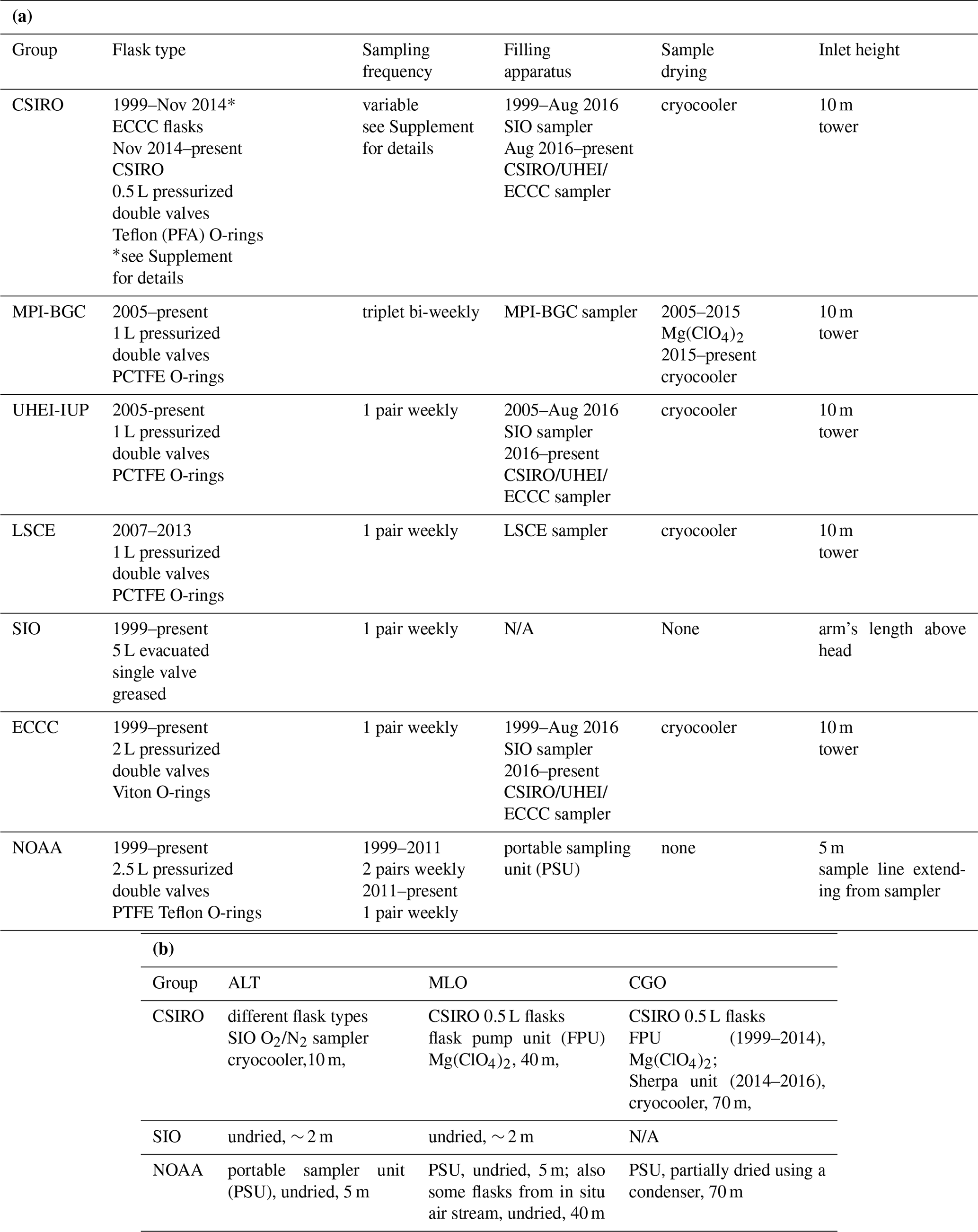
Table 3 Flask air collection schedule for each participating laboratory at ALT.

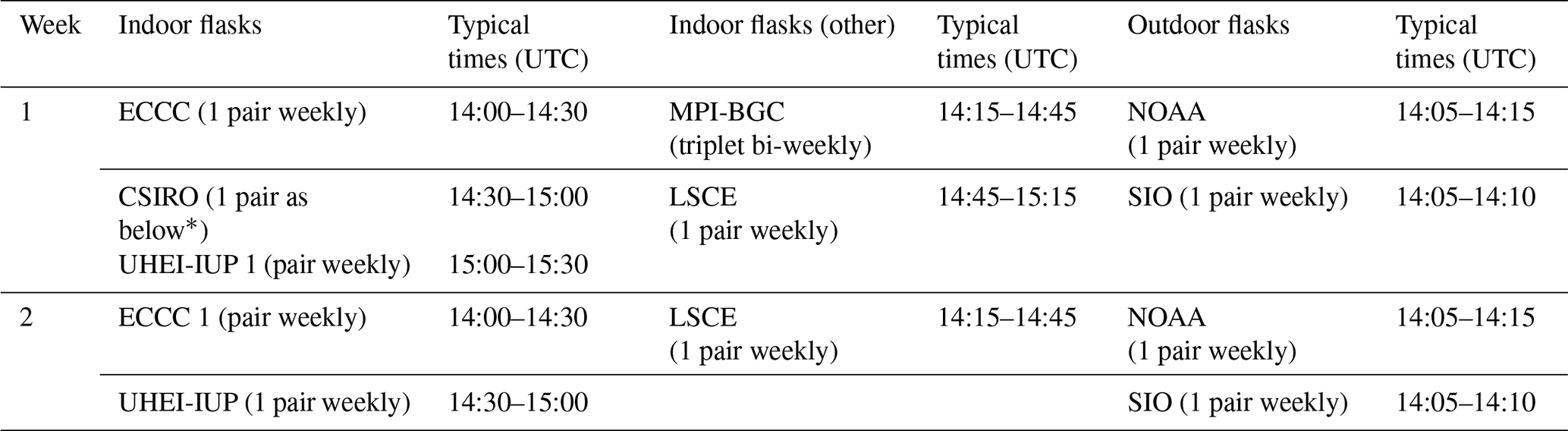
^∗ CSIRO: biweekly from Nov to May; weekly rest of the year.

2.3.3 Sampling conditions

Table 3 provides the coordinated ALT weekly flask air collection schedule for participating laboratories. The coordinated sampling schedule was devised to ensure that the flask samples for each individual laboratory are collected on the same day and as close in time as possible, within a 2 h window. Small variations in sampling time are unlikely to result in notable discrepancies. Flask air samples were collected at Alert during persistent southwesterly wind conditions, when wind speeds were greater than 1.5 m s⁻¹ for several hours prior to sample air collection. If conditions were unsuitable on the regular sampling day (Wednesday), sampling would be postponed to the following day. If conditions remained unfavorable by Friday, sampling would proceed, but it was acknowledged that conditions were suboptimal.

At MLO, sampling for all laboratories (NOAA, CSIRO and SIO) was conducted within an hour of each other and prior to noon (local time) in an effort to avoid upslope, non-baseline wind conditions at the site.

At CGO for NOAA and CSIRO, sampling was predominantly carried out under baseline conditions of 190–280^∘ N wind direction and wind speeds exceeding 5 ms⁻¹ wind speed, or the data were subsequently filtered for baseline conditions.

2.4 Instrumentation and analytical methods

Instrumentation and methods used to measure the flask air samples collected at the sampling sites vary between the laboratories and continue to evolve within each laboratory. To the extent possible, each laboratory handles the flask air samples and measurements in the same way as other flasks from their observing network. Table 4 summarizes each laboratory's analytical instrumentation and calibration scales used for each species, for the period of this study. A brief summary of the instrumentation is provided below, and calibration scales will be discussed in more detail in “Results and discussion” (Sect. 3).

Table 4 Summary of types of instrumentation, repeatability, and scales used for the flask air analysis at each participating laboratory during the period of this study.

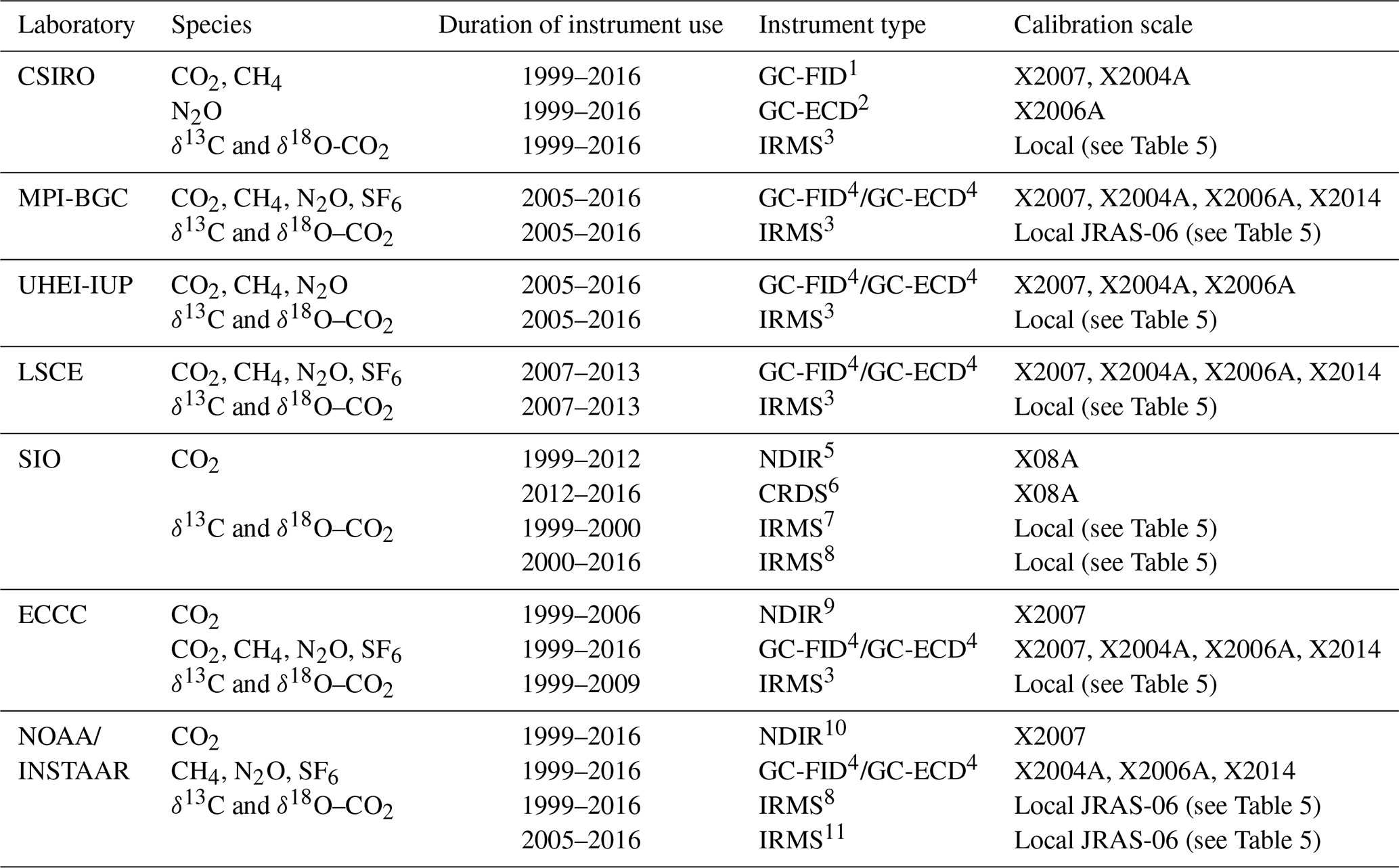
¹ Carle 400 (repeatability of 0.05 ppm for CO₂, 3 ppb for CH₄). ² Shimadzu (repeatability of 0.2 ppb for N₂O). ³ MAT252 (repeatability of 0.02 ‰ for δ¹³C–CO₂ and 0.04 ‰ for δ¹⁸O–CO₂). ⁴ Agilent 5890/6890/7890 (repeatability of 0.05 ppm for CO₂, 3 ppb for CH₄, 0.2 ppb for N₂O, and 0.04 ppt for SF₆). ⁵ APC model 55 (repeatability of 0.05 ppm for CO₂). ⁶ Picarro (repeatability of 0.01 ppm for CO₂). ⁷ VGII (repeatability of 0.02 ‰ for δ¹³C–CO₂ and 0.04 ‰ for δ¹⁸O–CO₂). ⁸ Micromass Optima DI (repeatability of 0.02 ‰ for δ¹³C–CO₂ and 0.04 ‰ for δ¹⁸O–CO₂). ⁹ Siemens Ultramat (repeatability of 0.05 ppm for CO₂). ¹⁰ Licor (repeatability of 0.05 ppm for CO₂). ¹¹ GV IsoPrime DI (repeatability of 0.02 ‰ for δ¹³C–CO₂ and 0.04 ‰ for δ¹⁸O–CO₂).

For CO₂, all laboratories except for NOAA and SIO used gas chromatography (GC) equipped with a nickel catalyst and flame ionization detector (FID) for the analysis of CO₂ in the flask air samples. The nickel catalyst converts CO₂ in the sample to CH₄, permitting analysis of CO₂ using the FID. NOAA used non-dispersive infrared (NDIR) spectroscopy throughout, and SIO used an NDIR until 2012 and then switched to a cavity ring down (CRDS) analyzer. The GC, NDIR, and CRDS systems have comparable analytical precision, ranging between 0.01 ppm (CRDS) and 0.05 ppm (GC).

For stable isotope ratio measurements of atmospheric CO₂, all participating laboratories used isotope ratio mass spectrometry (IRMS). Before introduction of the sample into an IRMS, the CO₂ in the air sample is first extracted using either an offline glass vacuum extraction system to prepare samples for later analysis (Bollenbacher et al., 2000; Huang et al., 2013) or using an online metal vacuum extraction system coupled directly to the mass spectrometer (Trolier et al., 1996; Werner et al., 2001; Allison and Francey, 2007) for analysis within 1 h of CO₂ extraction. All laboratories except ECCC and SIO used an online extraction approach; ECCC and SIO used an offline technique where pure CO₂ samples were flame-sealed in ampoules after extraction and stored for variable lengths of time, ranging from 1 month to 1 year before IRMS analysis (it has been verified at ECCC that the isotopic compositions of CO₂ in ampoules do not change within the range of accepted uncertainty during a storage time of > 10 years). All the laboratories used dual-inlet mode for δ¹³C and δ¹⁸O measurements but employed different strategies to link the individual sample measurements to the primary scale VPDB–CO₂. Table 5 details the various calibration strategies used and highlights the differences that exist between the laboratories. Since 2015, the WMO-GAW community has endorsed the JRAS-06 realization (Wendeberg et al., 2013; GAW Report, 2011) of the VPDB–CO₂ scale for reporting stable isotope measurements of atmospheric CO₂, but this has not been fully implemented by all laboratories. For further explanations of VPDB–CO₂ and JRAS-06, please see Sect. 3.2. For each laboratory, the repeatability of δ¹³C–CO₂ and δ¹⁸O–CO₂ measurements are typically less than 0.02 ‰ and 0.04 ‰ (1σ), respectively.

For CH₄, all participating laboratories used gas chromatography (GC) with flame ionization detection (FID) for analysis of CH₄, with typical analytical repeatability of less than 3 ppb. For N₂O and SF₆, all participating laboratories used gas chromatography (GC) equipped with an electron capture detector (ECD) for analysis of N₂O and SF₆ in the weekly collected flask air samples. The analytical repeatability for N₂O and SF₆ using GC–ECD is typically 0.2 ppb and 0.04 ppt respectively.

Table 5 Summary of δ¹³C–CO₂ and δ¹⁸O–CO₂ scale propagation and calibration strategies employed by each participating laboratory.

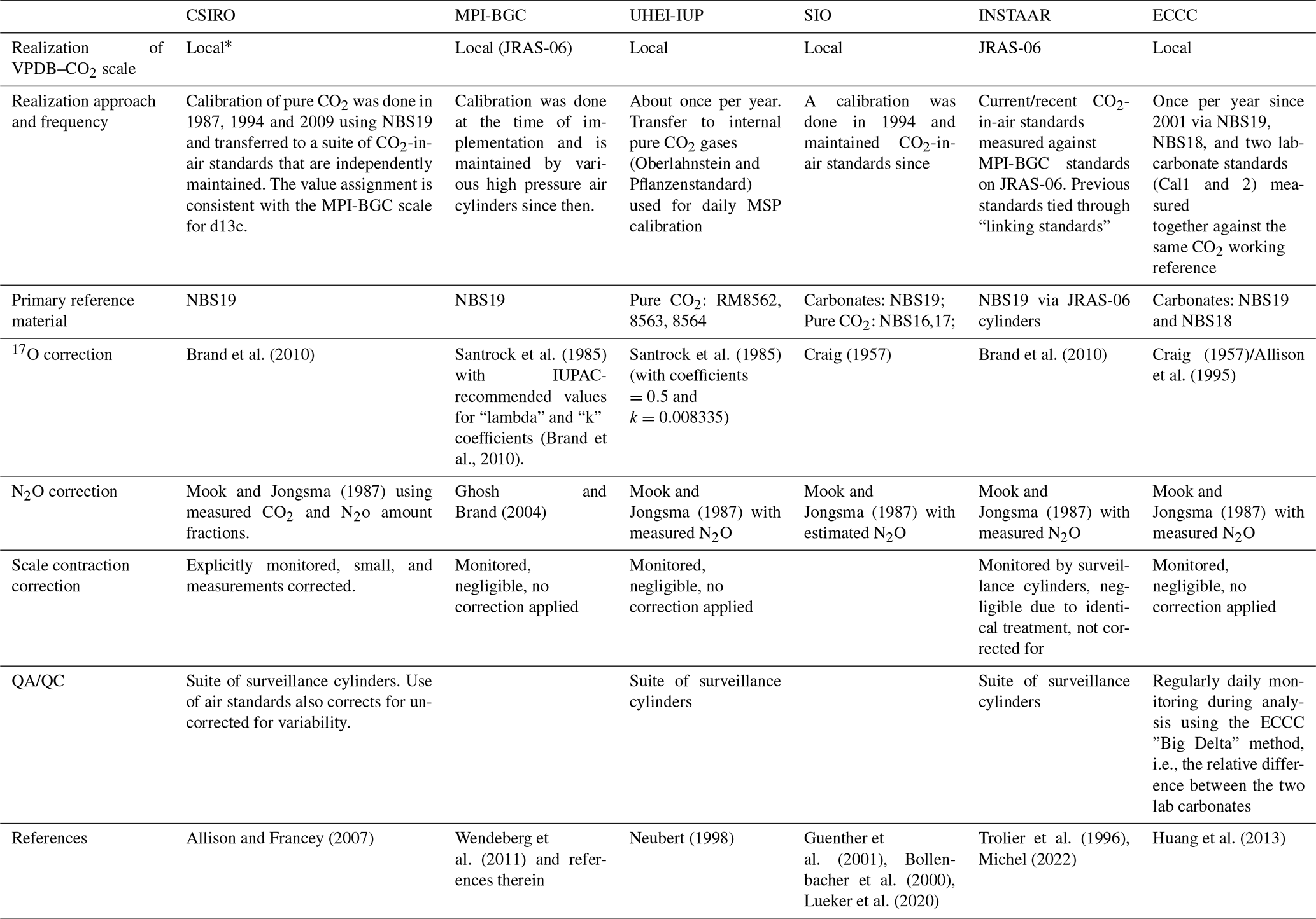
^∗ A realization of VPDB via an MPI-BGC value-assigned tank and revisions to all CSIRO data is in progress.

2.5 Data preparation

All measurements used in this study have been screened by the originating laboratory to ensure that each sample and subsequent measurement have not been compromised during collection, storage, and analysis. Each laboratory determines their own criteria for the quality control of their data and assigns the flags “valid”, “invalid”, or “suspected”. These data files were provided to us by individual laboratories and have specific time stamps, which can be found in the Supplement and Table S2. These time stamps identify the state of the data used in this study, in terms of scale updates/corrections, etc., which is important information because the same datasets may be found in other data repositories as updated versions with scale changes and/or modifications. As the data preparation is critical to the results, we describe the detailed methods for data preparation used in this study in the following sections.

Data matching and reference time series. To match the appropriate co-located and same-flask measurements from the seven laboratories for comparison, participants agreed to submit measurement results that include information on sample collection time (in coordinated universal time (UTC)), collection method, flask identification, measurement value, quality control flag, and analytical instrument identification. Matching algorithms identify and separate same-flask measurements (samples with identical collection date/time and container ID) from co-located measurements. All data that have been flagged as “valid” by each individual laboratory are used.

All same-flask measurements from ALT are differenced from measurements by ECCC, on a one-to-one basis (i.e., laboratory minus ECCC). All co-located flask measurements from ALT, CGO, and MLO are differenced from the reference time series of NOAA for CO₂, CH₄, N₂O, and SF₆ and INSTAAR for δ¹³C and δ¹⁸O of CO₂ (laboratory minus NOAA or INSTAAR). Ideally, the reference time series should demonstrate consistency over the entire comparison period, have minimal gaps, and accurately represent the true abundance of the atmospheric trace gas constituents at the sites. In practice we do not have a single laboratory who we know to be the truth, so we must choose one that best meets our requirements. NOAA and INSTAAR were chosen because their records span the entire period of our study with minimal data gaps. Also, by hosting the WMO Central Calibration Laboratory for CO₂, CH₄ and N₂O, NOAA is well placed to assess measurements on the WMO scales and INSTAAR, by virtue of their close association, is an appropriate choice for the stable isotopes of CO₂. Further, NOAA/INSTAAR has extensive and well-documented quality control procedures in place to ensure internal consistency of its measurements (Conway et al., 1994; Dlugokencky et al., 1994; Trolier et al., 1996).

Co-located data pool and analyses. Prior to any ALT, CGO, and MLO co-located analyses, data pools were created for each site and species, consisting of no more than two valid measurements from each laboratory (including NOAA and INSTAAR) for each day of sampling (sampling episode). Since most participants collect a pair of air samples during each sampling episode, two measurement results are typically available. When more than two valid measurements exist for a given sampling episode from a laboratory, we select two at random from the set of available measurements. For example, three (and sometimes four) MPI-BGC flask air samples are collected during each sampling episode at Alert, so two measurements are selected at random from the available valid MPI-BGC measurements and added to the data pool. If there is only one valid measurement available from one of the laboratories, we do include that single sample in the data pool. This data pool process allows for a more equal representation for all laboratories. The first analysis performed using the ALT data pool was the calculation of mean flask pair differences for CO₂, δ¹³C–CO₂, δ¹⁸O–CO₂, CH₄, N₂O, and SF₆ for each participating laboratory, and these can be found in Tables S3 to S8. These flask pair differences could be used as a proxy of individual lab uncertainties. The discussion of these differences will be found in future sections.

For all sites, each laboratory's individual data points in the pool are differenced from the reference time series data in the same pool (i.e., NOAA or INSTAAR). In most cases, the reference time series has two data points, which are averaged and that value is then differenced from each point of the other laboratory. If the reference time series has only one data point for a certain sampling episode, that single point is used for each point of the other laboratory. Our co-located comparison strategy produces a set of difference time series (laboratory minus reference) for each individual trace gas species and isotope measurement record. Before analyzing the time series, we first examined characteristics of their distributions and found that, in general, they are not normally distributed (non-parametric). The statistical approach carried out in this study is based on the assumption of non-normal distributions. It is quite common to observe a pattern of systematic differences (bias) that can be persistent for many months and then change either abruptly or gradually into a different pattern. Thus, we summarize each distribution of individual differences using annual median values with an estimate of the 95 % confidence interval (CI), which makes no assumptions about the distribution of the “true” difference population. The 95 % CI is computed using methods described by Campbell and Gardner (1988). In this way, our initial statistics should not be unduly influenced by outliers. The final derived annual median deviations are compared to the target goals outlined by the WMO-GAW greenhouse gas program to assess the level of agreements of individual datasets with the reference laboratory.

2.6 Level of agreement between multiple measurement records

In addition to the assessment of individual laboratory co-located comparisons, we attempt to estimate the overall level of grouped agreement from multiple measurement records for each species using two approaches. The first approach provides the 95th percentiles of the individual differences of all laboratory's measurements relative to NOAA's or INSTAAR's corresponding observation. However, because variations in NOAA's or INSTAAR's observational records might impact the results, we also report a second proxy for the level of grouped agreement, i.e., 2 standard deviations (2σ) from the means of each weekly sampling episode, which would define a region that includes 95 % of all the measurement values. Although less susceptible to bias by NOAA or INSTAAR, this grouped proxy is also not ideal because the introduction of new programs could potentially alter the mean and hence the 2σ of the group. In addition, the use of 2σ values is less reliable than using percentiles for skewed distributions. But by providing both measures for the level of agreement, we hope that any limitation of one measure over the other can be compensated when interpreting them together. The values determined by both methods reflect the overall maximum bias between the measurement records from multiple monitoring programs.

2.7 Data visualization

For each trace gas and isotope comparison, we have prepared one figure (Figs. 1–6), consisting of several graphs each. For CO₂, δ¹³C–CO₂, δ¹⁸O–CO₂, CH₄, and N₂O, the figures include five graphs each, from (a) to (e), but for SF₆ there are only four graphs labeled (a) to (d). These figures, along with three data summary tables, are designed to facilitate visualizing and interpreting our results. Graph (a) in these figures displays the time series of each laboratory's measurements. It highlights the long-term trend, seasonal patterns, and natural variability in the records and provides context for the comparison results. Graph (b) consists of several panels, each showing the individual co-located measurement difference (laboratory minus reference) for each laboratory. Differences exceeding the graph's y axis range are plotted with an “X” symbol; however, these data points are still included in all analysis procedures. The dark shaded band, which is also shown in graphs (c)–(e), represents the WMO-GAW-recommended target of measurement agreement for well-mixed air at remote sites in the Northern Hemisphere. Results from past WMO/IAEA Round Robin experiments (Global Monitoring Laboratory – Carbon Cycle Greenhouse Gases (https://gml.noaa.gov/ccgg/wmorr/index.html, last access: 17 November 2023)) are plotted as differences (laboratory minus NOAA or INSTAAR) with yellow triangles, representing each laboratory's level of consistency with the reference lab on scale at the time of the experiment. Table S1 shows round robin differences versus NOAA or INSTAAR for all laboratories over the time period (only RR data that are on the same scale as data in the paper have been included). Graph (c) shows, for each laboratory, the annual medians of the differences plotted in graphs (b) with the lower and upper limits of estimated 95 % confidence intervals (CI). The fourth graph, Graph (d), for all species except SF₆, shows the same analysis as that done at Alert in graphs (c) but for the co-located comparison experiments between SIO, CSIRO, and NOAA at MLO and between CSIRO and NOAA at CGO. Graph (d) for SF₆ is the same as Graph (e) for the others, which shows the individual co-located measurement difference (laboratory minus reference) for all the laboratories as a collective. The blue line shows annual values of 95th percentile ranges (2.5th and 97.5th), and the pink line shows annual means of 2σ for the weekly sampling episodes. For comparison purposes, we have included the annual means, shown in yellow, of the 2σ for the combined weekly sampling episodes between CSIRO, SIO, and NOAA at MLO.

In addition to the main figures and tables, supplementary figures and tables are included for some species when applicable.

3 Results and discussion

As we consider results from 17 years of comparison experiments at Alert, a practical indicator of success is if the measurement agreement reported here falls within the WMO-GAW-recommended target levels for network consistency based on well-mixed background air records (GAW Report, 2020). In other words, it could be assumed that using these records together would not introduce significant uncertainties, if the agreement between independent Alert atmospheric records is consistently within the WMO-GAW measurement agreement goal over the study period.

In this work, we assess the level of agreement for those individual measurement records at Alert by evaluating the differences related to the reference time series and evaluate these differences as annual and overall median values. When persistent differences exceed the WMO-GAW-recommended targets, we then consider results from same-flask and same-cylinder experiments to confirm the differences if data are available. To support the results at Alert, the corresponding comparisons at MLO and at CGO are also evaluated.

We recognize that, for some species, the network comparison goals may not be currently achievable within current measurement and/or scale transfer uncertainties and that these goals are targeted for application areas which require the smallest possible bias among different datasets for the detection of small trends and gradients. However, there are, of course, other application areas where such tight comparison goals may not be required, such as in urban emission estimates, long-term trend analysis, as well as in some regional modeling studies where uncertainties in air transport, for example, overshadow measurement uncertainties. Our work in this study could provide more confidence on the uncertainty estimation for these applications as well.

3.1 CO₂

All measurements are reported in this paper relative to the WMO X2007 CO₂ mole fraction scale (Zhao and Tans, 2006), except for those from SIO, which are reported on the SIO X08A scale (Keeling et al., 2016). This data analysis was completed prior to the latest scale upgrades by NOAA (as the WMO Central Calibration Laboratory) to the WMO X2019 scale and by SIO to the SIOX12A scale. Future comparisons within the WMO community should evaluate the implementation of these new scales. Measurements of atmospheric GHGs are reported in units of dry air mole fraction. CO₂ is reported as micromoles CO₂ per mole of dry air (µmol mol⁻¹), abbreviated ppm.

As noted above, Fig. 1a shows the individual co-located atmospheric CO₂ measurement records from air samples collected at Alert (1999–2016). For reference, the average flask pair difference and 1σ (standard deviation) for each individual laboratory can be found in Table S3. Figure 1b shows individual co-located measurement differences (laboratory minus NOAA) along with the darkly shaded WMO-recommended target level of ± 0.1 ppm CO₂. Results from the WMO/IAEA Round Robin experiments spanning this period are indicated by yellow triangles. The annual median values with 95 % CI for each laboratory's difference distribution are shown in Fig. 1c. A summary of these results is listed in Table S9.

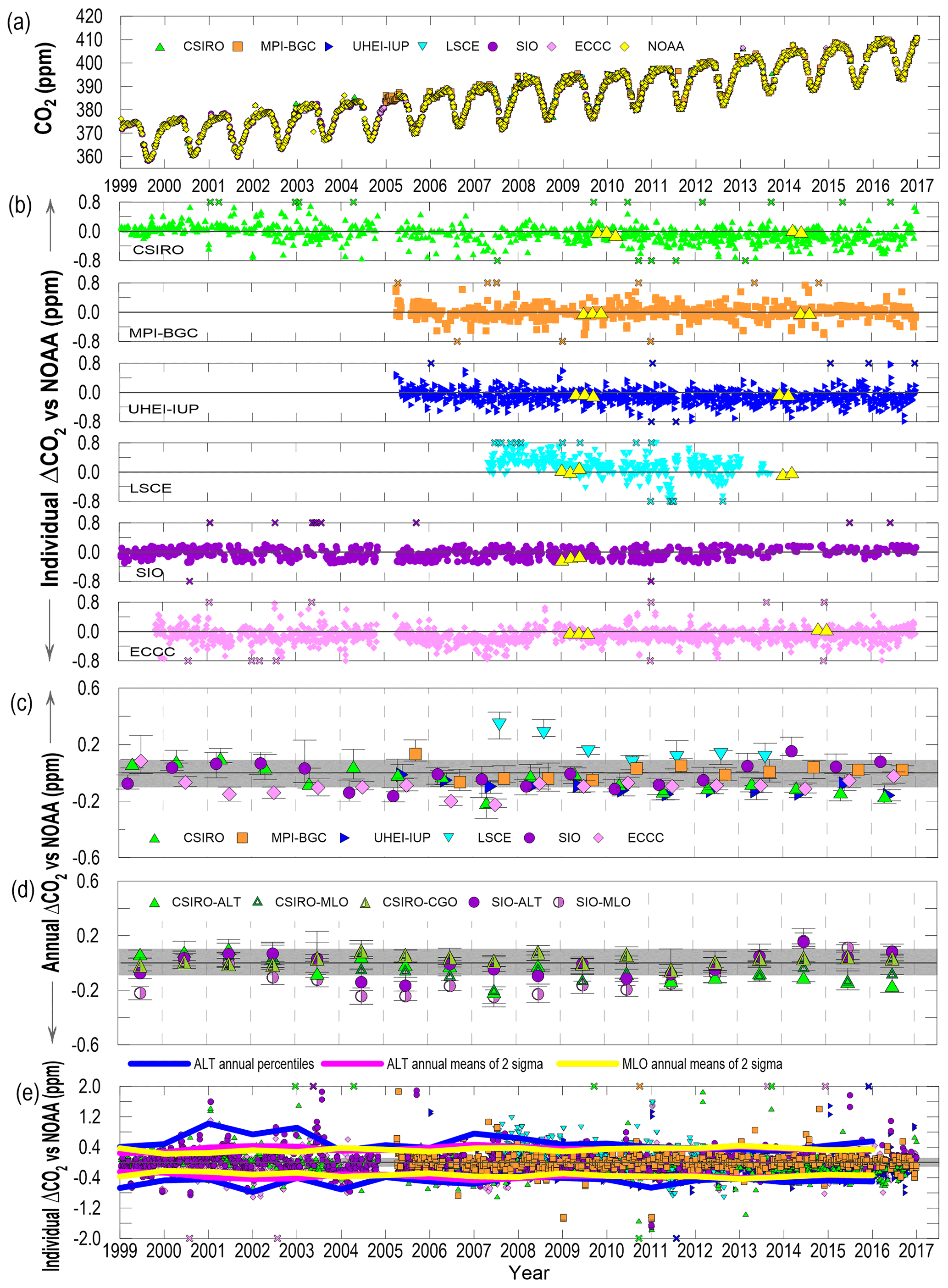
Figure 1 Atmospheric CO₂ comparison results (in ppm) from flask samples taken at Alert, Canada (ALT), Mauna Loa, USA (MLO), and Cape Grim, Australia (CGO) by seven laboratories (CSIRO, MPI-BGC, UHEI-IUP, LSCE, SIO, ECCC, and NOAA). (a) Time series of each laboratory's measurements at ALT, showing long-term trends and seasonal patterns in the records. (b) Individual ALT CO₂ measurement differences (laboratory minus NOAA) (in ppm). Differences exceeding the y-axis range are plotted with an “X” symbol on the outer axis. Results from the WMO/IAEA Round Robin experiments are overlaid in yellow triangles. The shaded grey band around the zero line indicates the WMO-GAW-recommended measurement agreement goal of ±0.1 ppm CO₂. (c) Annual median CO₂ differences (laboratory minus NOAA) at ALT in ppm, with the lower and upper limits of estimated 95 % confidence intervals (CI). (d) Annual median CO₂ differences and 95 % confidence limits (in ppm) of CSIRO minus NOAA at MLO and CGO, and SIO minus NOAA at MLO. Also included are results from ALT in (c). (e) Individual measurement differences (laboratory minus NOAA) at ALT (in ppm) for all the laboratories as a collective. Differences exceeding the y-axis range are plotted with an “X” symbol on the outer axis (some extreme outliers have been removed to produce the results). The annual 2.5th and 97.5th percentiles of the entire difference distribution from all laboratories at ALT are shown in blue (from −0.51 to +0.53 ppm). The pink lines show the annual means of the CO₂ ± 2σ variations of weekly sampling episodes at ALT (± 0.37 ppm), and the yellow lines show the annual means of the CO₂ ± 2σ variations of weekly sampling episodes at MLO (± 0.34 ppm).

The overall (1999–2016) median difference of all available individual measurements from each laboratory relative to NOAA (Table S9) suggests that the CSIRO, MPI-BGC, SIO, UHEI-IUP, and ECCC CO₂ records from Alert are consistent with the NOAA record to close to the WMO-recommended ± 0.1 ppm CO₂ window at the 95 % CI. However, it is important to be aware that at higher temporal resolution, e.g., yearly, we often observe median differences that exceed the WMO target for one or more consecutive years. As an example, ECCC has a persistent bias of approximately −0.14 ppm from 2001–2007, which is then reduced in 2008. UHEI-IUP meets the WMO-recommended target window from 2005–2008 but has a bias of approximately −0.13 ppm from 2009–2016; the reason for these differences is unclear. An instrument change by SIO in 2012, from an NDIR to a CRDS analyzer, can be seen as a slight reduction of noise in the difference data (Fig. 1b), and the results seem to be slightly more positive after the change, but the results are still within the WMO target. Measurement differences between LSCE and NOAA show that LSCE is consistently high relative to NOAA, resulting in annual differences that exceed the WMO target. However, if we exclude results from the first two comparison years, the LSCE median value offset appears stable at approximately +0.11 ppm CO₂. These findings are consistent with annual median results from the same-flask comparison at Alert, where LSCE measurements tend to be greater than ECCC measurements of the same-flask sample (Fig. S1 and Table S10). The overlaid WMO Round Robin results (Fig. 1b, Table S1) show reasonable consistency between the LSCE internal scale and the WMO CO₂ mole fraction scale.

Figure S2 shows median differences (laboratory minus NOAA) by month for each laboratory using data from the entire 17-year period. Overall, with the exception of SIO, we found no obvious evidence of significant seasonal bias in the co-located CO₂ difference distributions. The SIO measurements relative to NOAA during the May–September period relative to the October–March period possibly showed a bias on the order of 0.25 ppm. A similar monthly analysis (not shown here) using results from the SIO and NOAA co-located comparison experiment at Mauna Loa (MLO) did not show a similar seasonal bias result, suggesting that the observed seasonal bias between SIO and NOAA at Alert may be unique to this site. The reason for this is unclear; the sampling at both sites is very similar.

Figure 1d provides the results from similar co-located comparison experiments between CSIRO, SIO, and NOAA at MLO and at CGO, which are plotted with the results from Alert. Table S11 shows that the overall median difference of all individual measurements of CSIRO relative to NOAA is −0.07 (95 % CI: −0.09, −0.04 ppm) at MLO and 0.03 (95 % CI: 0.02, 0.03 ppm) at CGO, respectively, which are relatively consistent with our findings at Alert of −0.05 (95 % CI: −0.06, −0.03) ppm. Also included in the figure are results from co-located comparison experiments between SIO and NOAA at MLO where the overall median difference is −0.11 (95 % CI: −0.13, −0.10) ppm CO_2. This difference is larger than our findings at Alert of −0.02 (95 % CI: −0.04, −0.01) ppm, but it is still close to the target window of ± 0.1 ppm.

Figure 1e shows individual co-located CO₂ measurement differences (in ppm) relative to NOAA for all the laboratories as a collective. Differences exceeding the y-axis range are plotted with an “X” symbol on the appropriate extreme axis. For the approach of using the 2.5th and 97.5th percentiles of the aggregated differenced data (laboratory minus NOAA), an overall collective agreement level of −0.51 to +0.53 ppm (N=5691) was found for the seven laboratories. The corresponding data can be found in Table S12. For the approach of using annual means of the 2σ variation of weekly sampling episodes, an overall measurement agreement is within the ± 0.37 ppm window (N=923) also at 95 % of CI. For comparison purposes, we have included the annual means of the combined 2σ variation results at MLO (Fig. 1e and Table S12) shown as the yellow lines (no individual data points are shown) with a comparable result of ± 0.34 ppm (N=905).

The observed measurement differences (as annual medians) found in this study can also provide a first estimate of time-dependent uncertainties of observations from a single laboratory. To assess the impacts of those uncertainties on related applications (e.g., long-term trend analysis), we estimate long-term trends of CO₂ from the six individual datasets (CSIRO, MPI-BGC, UHEI-IUP, SIO, ECCC, NOAA) for various 11- and 12-year time periods (2005–2016, 2005–2015, 2006–2016) via Nakazawa's curve-fitting routine (Nakazawa et al., 1997). Table S13 shows very consistent results for these applications. The long-term increases in CO₂ concentrations are 23.62 (2.15 ppm yr⁻¹) ± 0.40 ppm (2σ) for 2005–2016, 21.11 ± 0.38 ppm (2σ) for 2005–2015, and 20.87 ± 0.22 ppm (2σ) for 2006–2016, respectively. The relative differences between the independent datasets are within a narrow range of 1.5 %–2.4 %, indicating that reliable results can be achieved from these individual datasets for long-term trend analysis (> 10 years). It is likely that much larger relative uncertainties would be involved in annual growth rate determination using the corresponding datasets.

3.2 δ¹³C of CO₂

Stable carbon isotopic ratio measurements in CO₂ are reported commonly as delta values (McKinney et al., 1950; Craig, 1957; Faure, 1986; O'Neil, 1986; Gonfiantini, et al., 1995; Coplen, 1994; Hoefs, 2015; Trolier et al., 1996). A delta value defined here is the relative deviation of two isotopic ratios between a sample and the standard, i.e., the primary VPDB–CO₂ or VPDB scale (VPDB: Vienna Pee Dee Belemnite). As the numerical value of a relative deviation is usually very small (close to 10⁻³), it is normally multiplied by 10³ and expressed in per mill (‰) as in the following relationship (Coplen, 1994; Coplen et al., 2002):

$$\begin{array}{rl}& {{\mathit{\delta }}^{\mathrm{13}}\mathrm{C}}_{\mathrm{samp}/\mathrm{VPDB}-\mathrm{CO}\mathrm{2}}=\left[\left({\left({}^{\mathrm{13}}\mathrm{C}{/}^{\mathrm{12}}\mathrm{C}\right)}_{\mathrm{sample}}/\right.\right.\\ & \left.\left.{\left({}^{\mathrm{13}}\mathrm{C}{/}^{\mathrm{12}}\mathrm{C}\right)}_{\mathrm{VPDB}-\mathrm{CO}\mathrm{2}}\right)-\mathrm{1}\right]\times {\mathrm{10}}^{\mathrm{3}}\mathrm{‰}.\end{array}$$

There is no single approach to the realization of the VPDB scale amongst individual laboratories (Table 5); in other words, although the laboratories have created local scales relative to VPDB through a link to NBS19, small inaccuracies in establishing this link may introduce scale differences between the measurement records. This should be kept in mind while interpreting the differences between the data records.

Figure 2a shows the individual co-located atmospheric δ¹³C–CO₂ measurement records at Alert (1999–2016), and Fig. 2b shows individual co-located measurement differences (laboratory minus INSTAAR) by laboratories. The average overall flask pair difference and 1σ standard deviation for each individual laboratory can be found in Table S4. The overall median difference results (Fig. 2c, Table S14) seem to show that ECCC's δ¹³C–CO₂ records from Alert agree with INSTAAR to within ± 0.01 ‰ at the 95 % CI, although the comparison period was relatively short (1999–2009) and the results change in both directions. Similar to the CO₂ results discussed previously, it is again important to be aware that at higher time resolution, we observe periods where the differences significantly exceed the WMO target and show changes in sign that persist for 1 or more consecutive years. For SIO, we observe a persistent positive offset between SIO and INSTAAR measurements with a median of 0.03 (95 % CI: 0.02, 0.03) ‰, which exists for much of the comparison period. We also observe that while the overall median differences for CSIRO, MPI-BGC, and UHEI-IUP relative to INSTAAR exceed the WMO target window with persistent negative biases ranging from −0.02 to −0.03 (95 % CI: −0.04, −0.02) ‰, the results suggest that the Alert δ¹³C–CO₂ records from these three laboratories show more agreement with each other than with the INSTAAR reference. It is noted that INSTAAR's measurements are linked to the VPDB–CO₂ scale through the calibrations performed by MPI-BGC (the WMO Central Calibration Laboratory: CCL) via the JRAS-06 realization. The agreement between INSTAAR and MPI-BGC appears to be better after 2015; however, prior to 2015, a bias seems to persist (Fig. 2c). As more laboratories within the community move towards linking their isotopic measurements of air CO₂ to the VPDB–CO₂ scale through the JRAS-06 realization and more comparison results are ultimately expanded over longer time periods and at larger spatial scales, this may improve our ability to assess some of the issues we are currently experiencing. All LSCE annual median values exceed the target window and show that LSCE co-located measurements are consistently more negative relative to INSTAAR with an overall median difference of −0.15 (95 % CI: −0.16, −0.14) ‰ over the available period (2007–2013). LSCE is aware of ongoing issues with the traceability of their laboratory scale, which likely accounts for the observed results. Thus, we exclude LSCE measurements from our estimate of the grouped measurement agreement (discussed later). It is also noticed that based on T test results (not shown), the calculated mean differences between laboratories and INSTAAR are statistically significant for almost all of the labs, although they are small; these results indicate that systematic differences do exist, which likely include scale realization differences.

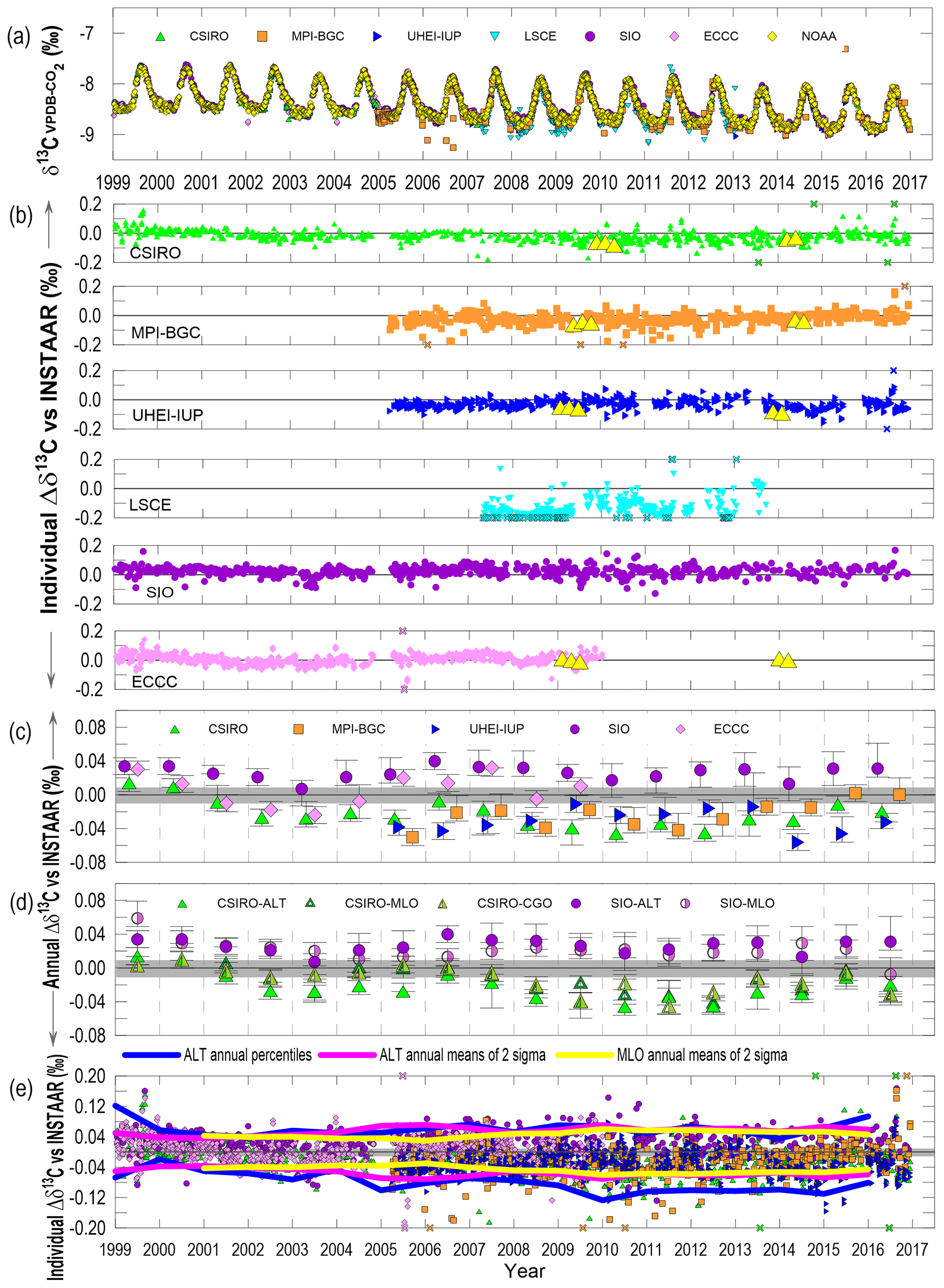
Figure 2 Atmospheric δ¹³C–CO₂ comparison results, in per mill (‰), from flask samples taken at ALT, MLO, and CGO by seven laboratories. (a) Time series of each laboratory's measurements at ALT, showing long-term trends and seasonal patterns in the records. (b) Individual ALT δ¹³C–CO₂ differences (laboratory minus INSTAAR) (in ‰). Differences exceeding the y-axis range are plotted with an “X” symbol on the outer axis. Results from the WMO/IAEA Round Robin experiments are overlaid in yellow triangles. The shaded grey band around the zero line indicates the WMO-GAW-recommended measurement agreement goal of ± 0.01 ‰. (c) Annual median δ¹³C–CO₂ differences (laboratory minus INSTAAR) at ALT (in ‰), with the lower and upper limits of estimated 95 % CI. (d) Annual median δ¹³C–CO₂ differences and 95 % CI (in ‰), of CSIRO minus INSTAAR at MLO and CGO, and SIO minus INSTAAR at MLO. Also included are results from ALT. (e) Individual measurement differences (laboratory minus INSTAAR) at ALT (in ‰) for all the laboratories as a collective. Some extreme outliers have been removed to produce the results. The annual 2.5th and 97.5th percentiles of the entire difference distribution from all laboratories at ALT are shown in blue (−0.09 ‰ to +0.07 ‰). The pink lines show the annual means of ± 2σ variations of weekly sampling episodes at ALT (± 0.06 ‰), and the yellow lines show the annual means of ± 2σ variations of weekly sampling episodes at MLO (± 0.05 ‰).

Analysis of the median differences by month for each laboratory relative to INSTAAR (not shown) over the available periods suggests there are no significant seasonal dependencies. We also note that corresponding results from available round robin experiments (Fig. 2b, Table S1) seem generally similar to the individual flask measurement differences from INSTAAR, which provides evidence that analytical procedure, calibration methods, and the approach for realization of the VPDB scale utilized by the participating laboratories may play an important role in the results.

Figure 2d and Table S15 show the similar co-located comparison experiments for δ¹³C–CO₂ between CSIRO, SIO, and INSTAAR at Mauna Loa (MLO) and between CSIRO and INSTAAR at Cape Grim (CGO). These results are also plotted with the results from Alert. The overall median difference of all individual measurements for δ¹³C–CO₂ (CSIRO minus INSTAAR) is −0.02 (95 % CI: −0.02, −0.01) ‰ at MLO and −0.01 (95 % CI: −0.01, −0.01) ‰ at CGO, respectively, which are fairly consistent with the findings at Alert of −0.03 (95 % CI: −0.03, −0.02) ‰. The corresponding median difference value of SIO from INSTAAR at MLO is 0.02 (95 % CL: 0.02, 0.02), which is also close to the values of 0.03 (95 % CL: 0.02, 0.03) at Alert.

For an estimation of the overall grouped measurement agreement among the six independent δ¹³C–CO₂ records at Alert (LSCE has been excluded), the results from two approaches are included in Fig. 2e. The estimated overall measurement agreement (Table S16) among the six independent Alert δ¹³C–CO₂ records is within the −0.09 ‰ to +0.07 ‰ window (n=3256). The pink lines in Fig. 2e represent the annual means of 2σ of each weekly δ¹³C–CO₂ sampling episode. The estimated overall measurement agreement among the six independent Alert δ¹³C–CO₂ records is within the range of ± 0.06 ‰ (n=899). For comparison purposes, the annual means of the 2σ values from MLO in Fig. 2e (yellow lines) and Table S16 show comparable results of ± 0.05 ‰ (n=756).

3.3 δ¹⁸O of CO₂

Oxygen isotopic ratio measurements in CO₂ are also commonly reported as delta values. A delta value is defined as the relative deviation of two isotopic ratios between a sample and the standard (i.e., the primary VPDB–CO₂ scale). Similar to δ¹³C, the numerical value of the relative deviation in δ¹⁸O is usually very small and is normally multiplied by 10³ and expressed in per mill (‰), as in the following relationship:

$$\begin{array}{rl}& {{\mathit{\delta }}^{\mathrm{18}}\mathrm{O}}_{\mathrm{samp}/\mathrm{VPDB}-\mathrm{CO}\mathrm{2}}=\left[\left({\left({}^{\mathrm{18}}\mathrm{O}{/}^{\mathrm{16}}\mathrm{O}\right)}_{\mathrm{sample}}/\right.\right.\\ & \left.\left.{\left({}^{\mathrm{18}}\mathrm{O}{/}^{\mathrm{16}}\mathrm{O}\right)}_{\mathrm{VPDB}-\mathrm{CO}\mathrm{2}}\right)-\mathrm{1}\right]\times {\mathrm{10}}^{\mathrm{3}}\mathrm{‰}.\end{array}$$

The “–CO₂” after VPDB indicates that the scale is linked via the CO₂ from the VPDB carbonate material by a standard procedure of acid digestion using phosphoric acid at 25 ^∘C (McCrea, 1950; O'Neil, 1986; Brand et al., 2009; Wendeberg et al., 2011; Huang et al., 2013). If the local scale used by different laboratories does not follow the same procedure, then δ¹⁸O–CO₂ results may not be compatible.

Figure 3a shows the individual co-located atmospheric δ¹⁸O–CO₂ measurement records at Alert (1999–2016), and Fig. 3b shows individual co-located measurement differences (laboratory minus INSTAAR) along with the recommended WMO target level of measurement agreement. For reference, the average flask pair difference and 1σ variability for each individual laboratory can be found in Table S5. The overall (1999–2016) median differences of all available individual measurements from each laboratory relative to INSTAAR (Fig. 3c, Table S17) show that the δ¹⁸O–CO₂ records by MPI-BGC and ECCC are each roughly compatible with the INSTAAR record to within the WMO-recommended ± 0.05 ‰ target window, and SIO and CSIRO are just slightly higher than the target at the 95 % CI (by 0.01 ‰ and 0.03 ‰, respectively). Similar to CO₂ and δ¹³C, larger systematic differences are observed in higher temporal-resolution windows and annual median values often exceed the WMO target in opposite directions. For example, for CSIRO's median differences from 1999–2009, the majority of the values fall within the target window. However, a positive bias of approximately 0.16 ‰ becomes noticeable from 2010 onwards. LSCE measurements tend to be more negative relative to INSTAAR with an overall median value of −0.12 (95 % CI: −0.15, −0.07) ‰, and UHEI-IUP measurements tend to be more positive relative to INSTAAR, with an overall value of 0.23 (95 % CI: 0.20, 0.27) ‰.

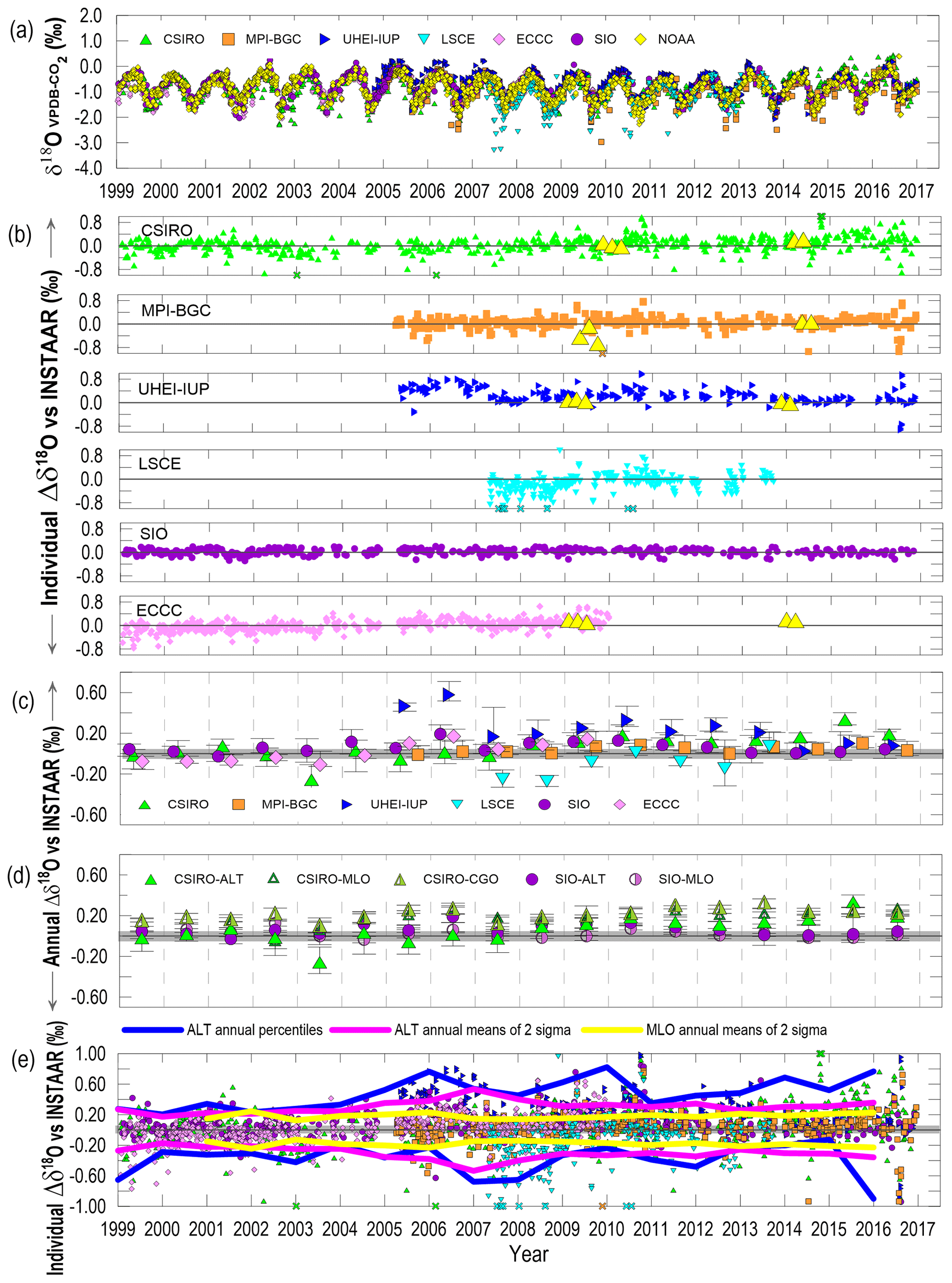
Figure 3 Atmospheric δ¹⁸O–CO₂ comparison results, in per mill (‰), from flask samples taken at ALT, MLO, and CGO by seven laboratories. (a) Time series of each laboratory's measurements at ALT, showing long-term trends and seasonal patterns in the records. (b) Individual ALT δ¹⁸O–CO₂ differences (laboratory minus INSTAAR) (in ‰). Differences exceeding the y-axis range are plotted with an “X” symbol on the outer axis. Results from the WMO/IAEA Round Robin experiments are overlaid in yellow triangles. The shaded grey band around the zero line indicates the WMO-GAW-recommended measurement agreement goal of ±0.05 ‰. (c) Annual median δ¹⁸O–CO₂ differences (laboratory minus INSTAAR) at ALT (in ‰), with the lower and upper limits of estimated 95 % CI. (d) Annual median δ¹³C–CO₂ differences and 95 % CI (in ‰), of CSIRO minus INSTAAR at MLO and CGO, and SIO minus INSTAAR at MLO. Also included are results from ALT. (e) Individual differences (laboratory minus INSTAAR) at ALT (in ‰) for all the laboratories as a collective. The annual 2.5th and 97.5th percentiles of the entire difference distribution from all laboratories at ALT are shown in blue (−0.50 ‰ to +0.58 ‰). The pink lines show the annual means of ± 2σ variations of weekly sampling episodes at ALT (± 0.31 ‰), and the yellow lines show the annual means of ± 2σ variations of weekly sampling episodes at MLO (± 0.19 ‰).

However, the overlaid available results from the periodic round robin experiments (Fig. 3b Table S1) show fewer differences than those in flask samples between INSTAAR and the individual laboratories, including CSIRO, MPI-BGC, UHEI-IUP, and ECCC; this infers that the larger differences observed in flask measurements might be due to variable moisture levels in the samples. Analysis of annual median differences by month for each laboratory relative to INSTAAR (not shown) does not suggest any seasonal dependencies.

Figure 3d and Table S18, respectively, show the results of δ¹⁸O–CO₂ from similar co-located comparison experiments between CSIRO and INSTAAR at Mauna Loa (MLO) and at Cape Grim (CGO), plotted with the results from Alert. The overall median difference of all individual measurements for CSIRO relative to INSTAAR is 0.18 (95 % CI: 0.17, 0.19) ‰ at MLO and 0.21 (95 % CI: 0.21, 0.22) ‰ at CGO, respectively. While the MLO and CGO results are more or less consistent with each other, they do not align with our overall findings at Alert, which show a value of 0.08 (95 % CI: 0.06, 0.10) ‰. However, as mentioned before, CSIRO's median at ALT from 2010 onwards (0.16 ‰) is fairly similar to the overall value at MLO from 1999 to 2016. Further data may be needed to make any comments on measurement consistency across entire networks for CSIRO and NOAA for δ¹⁸O–CO₂. The results between SIO and INSTAAR at Alert and at MLO show a consistent pattern in the difference distribution (SIO relative to INSTAAR) at both sites, with the overall median difference at MLO being 0.03 (95 % CI: 0.02, 0.04) ‰ and the median difference at Alert being 0.06 (95 % CI: 0.05, 0.08) ‰, and thus it is likely that the comparison results at first estimation are representative of measurement consistency across entire networks for SIO and INSTAAR.

Finally, we estimate a grouped measurement agreement among the seven independent Alert δ¹⁸O–CO₂ records by aggregating all individual differences from participating laboratories (relative to INSTAAR) to compute the 2.5th and 97.5th percentiles. This upper and lower limit contains 95 % of the entire difference distribution from all laboratories and represents our best estimate of measurement agreement (blue lines in Fig. 3e). Table S19 shows that the seven independent co-located δ¹⁸O–CO₂ records at Alert are compatible to within a −0.50 ‰ to +0.58 ‰ window (N=2738). For the approach of using the means of the 2σ variation from weekly sampling events through the entire period, the corresponding overall measurement agreement is within the range of ± 0.31 ‰ (n=872; pink lines in Fig. 3e). For comparison purposes the annual means of the 2σ values from MLO in Fig. 3e (yellow lines) and Table S19 show a smaller range of ± 0.19 (n=729) ‰.

3.4 CH₄

All CH₄ measurements are reported relative to the WMO X2004A CH₄ mole fraction scale, which is described by Dlugokencky et al. (2005) with updated information (2015) available at https://www.esrl.noaa.gov/gmd/ccl/ch4_scale.html (last access: 17 August 2022). Measurements of atmospheric CH₄ are reported in nanomoles (billionths of a mole CH₄) per mole of dry air and abbreviated ppb (parts per billion).

Figure 4a shows the individual co-located atmospheric CH₄ measurement records at Alert (1999–2016), and Fig. 4b shows individual co-located measurement differences (laboratory minus NOAA) along with the recommended target level of measurement agreement and round robin results. Figure 4c shows the annual median values with 95 % CI for each laboratory's difference distribution. The WMO-GAW-recommended target range is again represented by the dark grey band. Table S20 summarizes these results.

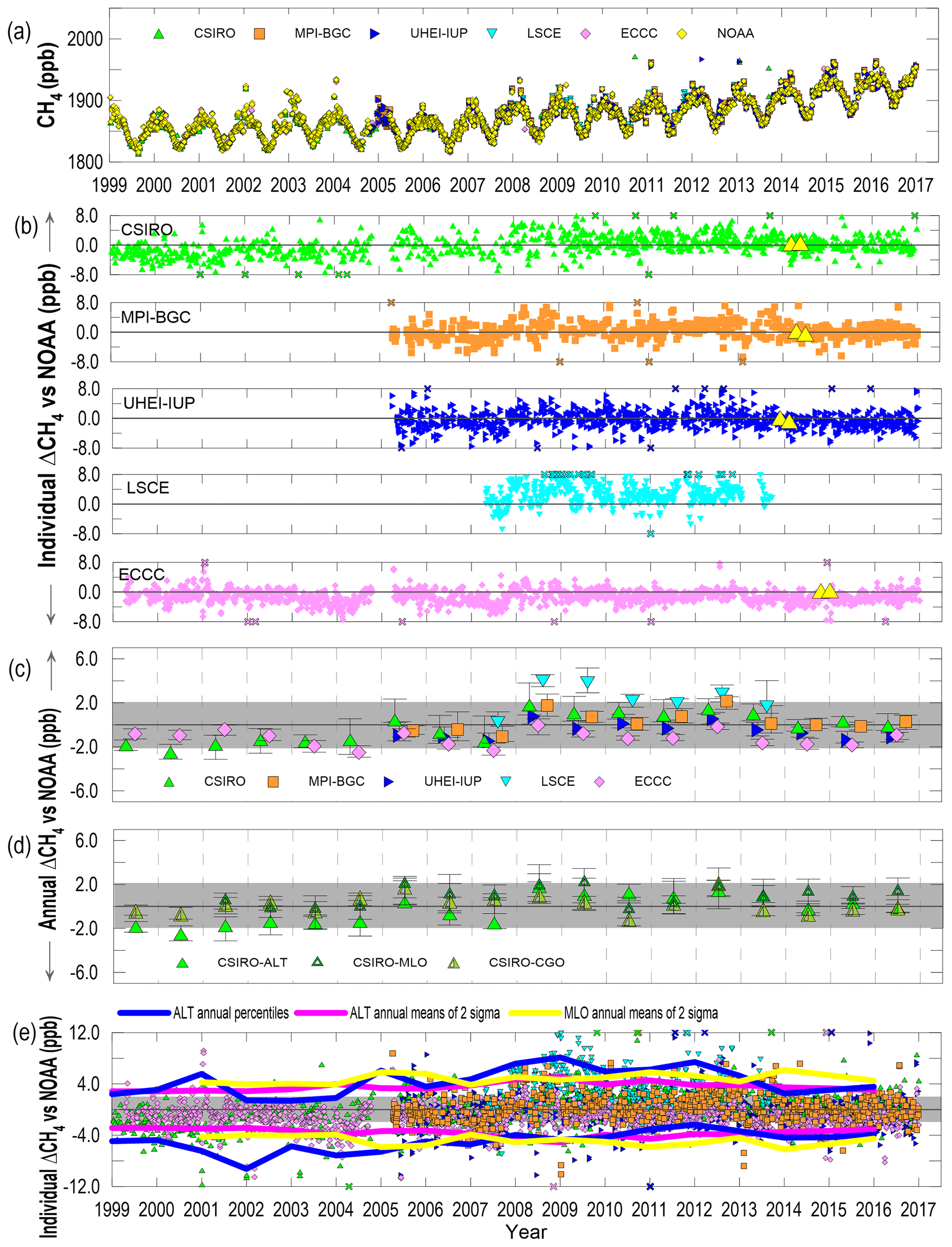
Figure 4 Atmospheric CH₄ comparison results (in ppb) from flask samples taken at ALT, MLO, and CGO by six laboratories (CSIRO, MPI-BGC, UHEI-IUP, LSCE, ECCC, and NOAA). (a) Time series of each laboratory's measurements at ALT, showing long-term trends and seasonal patterns in the records. (b) Individual CH₄ differences (laboratory minus NOAA) at ALT (in ppb). Differences exceeding the y-axis range are plotted with an “X” symbol on the outer axis. Results from the WMO/IAEA Round Robin experiments are overlaid in yellow triangles. The shaded grey band around the zero line indicates the WMO-GAW-recommended measurement agreement goal of ± 2.0 ppb. (c) Annual median CH₄ differences (laboratory minus NOAA) at ALT (in ppb) with the lower and upper limits of estimated 95 % CI. (d) Annual median CH₄ differences and 95 % CI (in ppb) of CSIRO minus NOAA at MLO and CGO. Also included are results from ALT. (e) Individual differences (laboratory minus NOAA) at ALT (in ppb) for all the laboratories as a collective. Some extreme outliers have been removed to produce the results. The annual 2.5th and 97.5th percentiles of the entire difference distribution from all laboratories at ALT are shown in blue (−4.86 to +6.16 ppb). The pink lines show the annual means of ± 2σ variations of weekly sampling episodes at ALT (± 3.62 ppb), and the yellow lines show the annual means of ± 2σ variations of weekly sampling episodes at MLO (± 4.88 ppb).

The overall (1999–2016) median difference of all available individual measurements relative to NOAA (Table S20) suggests that the CH₄ records of CSIRO, MPI-BGC, UHEI-IUP, and ECCC from Alert agree with NOAA within the WMO-recommended ± 2 ppb CH₄ compatibility target window. At higher resolution we sometimes observe differences that exceed the target window for 1 or more consecutive years, without known causes. For example, annual median differences between ECCC and NOAA generally show a consistent offset of approximately −1 ppb except 2003–2004 and 2007, where the offset lies slightly outside the target window. Similar results are observed between LSCE and NOAA where there is a consistent positive offset of ∼ 2 ppb except for 2008 and 2009, where the offset of ∼ 4 ppb lies outside the target window. MPI-BGC and UHEI-IUP show fairly consistent agreement versus NOAA throughout the time period, with just 1 year outside the target window for MPI-BGC in 2012. Annual differences for CSIRO show a slightly negative bias from 1999–2008 with 1 year outside of the target window and a more positive bias from 2009–2016.

Results from the periodic round robin experiments (Fig. 4b, Table S1) are consistent with the co-located comparison results for each individual participating laboratory. Analysis of annual median differences by month for each laboratory relative to NOAA (not shown) does not suggest any seasonal dependencies.

Results from similar co-located comparison experiments between CSIRO and NOAA at Mauna Loa (MLO) and at Cape Grim, (CGO) are plotted with the results from Alert in Fig. 4d. As shown in Table S21, the median difference of all individual CH₄ measurements from CSIRO relative to NOAA is 0.66 (95 % CI: 0.38, 0.88) ppb for MLO, 0.11 (95 % CI: −0.07, 0.32) ppb for CGO, and 0.01 (95 % CI: −0.19, 0.21) ppb for Alert, respectively. The results are all within the WMO-recommended compatibility target window. Therefore, the comparison results at the shared site such as Alert could be representative of measurement consistency across entire networks for CSIRO and NOAA for CH₄.

Finally, we estimate an overall measurement agreement among the six independent Alert CH₄ records of −4.86 to +6.16 ppb (N=4472) over the entire period of 1999–2016 (Table S22), shown in blue lines in Fig. 4e. For the approach of using the means of the 2σ variation from weekly sampling events through the entire period, the estimated overall measurement agreement among the six independent Alert CH₄ records is within the range of ± 3.62 ppb (n=887) (pink lines in Fig. 4e). For comparison, we have included the annual means of the combined 2σ variation results of ± 4.88 ppb (n=375) at MLO in yellow lines (Fig. 4e and Table S22).

3.5 N₂O

All N₂O measurements are reported relative to the NOAA 2006A N₂O mole fraction scale, which is described by Hall et al. (2007) with updated information (2011) available at https://gml.noaa.gov/ccl/n2o_scale.html (last access: 17 November 2023). Measurements of atmospheric N₂O are reported as a dry air mole fraction in nanomoles (billionths of a mole N₂O) per mole of dry air and abbreviated ppb (parts per billion). All N₂O measurements in this study were determined using GC–ECD analytical methodology. These systems typically achieved repeatability of 0.15 to 0.3 ppb, making the comparisons much noisier and, therefore, more difficult to evaluate whether the WMO target goal of ± 0.1 ppb has been achieved. Fortunately, several new spectroscopic methods are now available and capable of providing analytical repeatability of 0.04 to 0.1 ppb (O'Keefe et al., 1999; Griffith et al., 2012). These new methods have a potential to make comparisons less noisy and possibly easier to interpret.

Figure 5a–e and Tables S23–S26 provide the corresponding information for N₂O. The seasonal cycle is more clearly defined in the UHEI-IUP dataset (Fig. 5a) than in the other data records due to better precision on their specific GC–ECD. Analytical precision of atmospheric N₂O measurement is estimated using agreement between measurements of air collected in two flasks sampled on the same apparatus at the same time. Table S7 summarizes average flask pair agreement based on air samples collected at Alert. Using pair agreement to estimate short-term noise, we find UHEI-IUP and NOAA N₂O measurements of flask air with repeatability of 0.13 ± 0.08 ppb and 0.30 ± 0.26 ppb, respectively. The NOAA measurement is less precise because it is derived from a single aliquot of air whereas all other laboratories typically use an average of 2–4 aliquots of sample air. Both NOAA and INSTAAR are limited in the volume of sample that can be used for each of their analyses because of the very large suite of trace gas species measured from the NOAA flask air sample. This has a much more profound impact on estimated N₂O precision than for other trace gas species and isotopes.

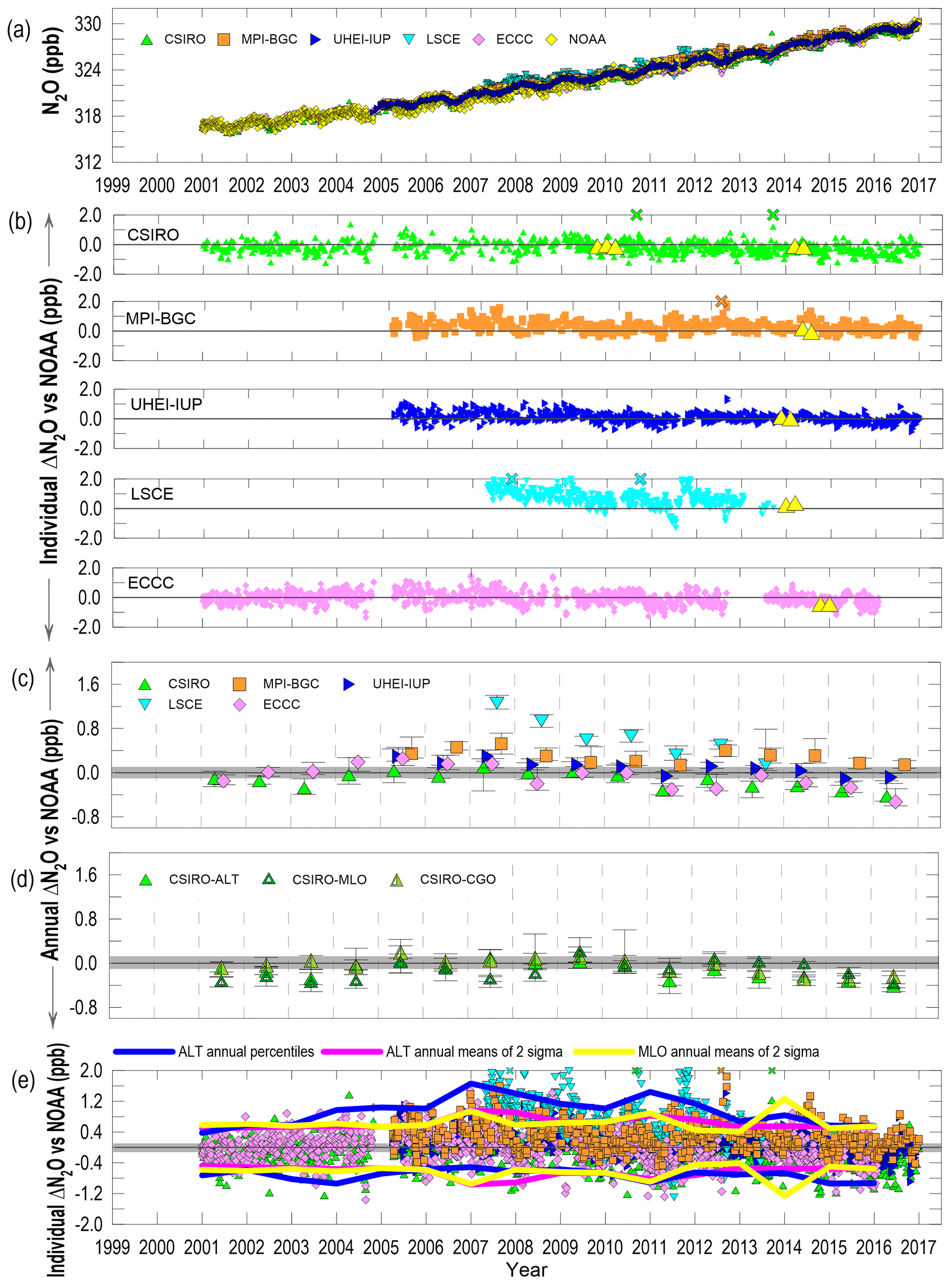
Figure 5 Atmospheric N₂O comparison results (in ppb) from flask samples taken at ALT, MLO, and CGO by six laboratories (CSIRO, MPI-BGC, UHEI-IUP, LSCE, ECCC, and NOAA). (a) Time series of each laboratory's measurements at ALT, showing long-term trends and seasonal patterns in the records. (b) Individual N₂O differences (laboratory minus NOAA) at ALT (in ppb). Differences exceeding the y-axis range are plotted with an “X” symbol on the outer axis. Results from the WMO/IAEA Round Robin experiments are overlaid in yellow triangles. The shaded grey band around the zero line indicates the WMO-GAW-recommended measurement agreement goal of ± 0.1 ppb. (c) Annual median N₂O differences (laboratory minus NOAA) at ALT (in ppb) with the lower and upper limits of estimated 95 % CI. (d) Annual median N₂O differences and 95 % CI (in ppb) of CSIRO minus NOAA at MLO and CGO. Also included are results from ALT. (e) Individual differences (laboratory minus NOAA) at ALT (in ppb) for all the laboratories as a collective. The annual 2.5th and 97.5th percentiles of the entire difference distribution from all laboratories at ALT are shown in blue (−0.75 to +1.20 ppb). The pink lines show the annual means of ± 2σ variations of weekly sampling episodes at ALT (± 0.64 ppb), and the yellow lines show the annual means of ± 2σ variations of weekly sampling episodes at MLO (± 0.64 ppb).

The overall (1999–2016) median difference of all available individual measurements from each laboratory relative to NOAA (Table S23) shows that the UHEI-IUP and ECCC N₂O records from Alert are roughly compatible with the NOAA record to within the WMO-recommended ± 0.1 ppb target window. However, as mentioned in each previous section, at higher resolution, we can observe median differences that well exceed the WMO target for many years. MPI-BGC differences show a consistently positive bias spanning from 2005 to 2014, which is reduced by approximately 2 fold in 2015–2016 when they switched from a Mg(ClO₄)₂ dryer to a cryocooler. MPI-BGC suggests that these impacts were mostly pronounced during the wetter summer months and attributes the issues to a change in the supplier of the Mg(ClO₄)₂. A similar problem was reported by Steele et al. (2007). There was no evidence of bias for any of the other trace species. Differences between LSCE and NOAA, which initially exceed the target by 1.2 ppb, steadily improve each year. By 2013, the final year of the comparison for LSCE, the annual median difference was improved by a factor of ∼ 10, to 0.15 ppb but still fell outside the WMO target window. Because the results from the same-flask comparison experiment between LSCE and ECCC (Fig. S3) show a similar difference pattern, this suggests that the sample collection process is not likely the cause of the observed co-located measurement differences. On the other hand, the sameflask air comparison results (Fig. S3, Table S24) for the other laboratories show that the median differences were mostly able to meet the target window, in contrast to the co-located comparisons, suggesting that there may be factors that are specific to the collection of the air itself causing some of the inconsistency among the various laboratories.

Results from the periodic round robin experiments (Fig. 5b, Table S1) are consistent with the co-located comparison results for each participating laboratory. With regard to seasonal dependencies, an analysis of median differences by month (not shown) displayed consistent offsets for each month indicating that the date of sample collection had no bearing on the annual results.

Earlier, we mentioned that analytical precision (estimated from flask pair agreement) of NOAA measurements is about a factor of 2 worse than UHEI-IUP measurements (see Table S7). To explore the impact this may have on our findings, we computed differences relative to the more precise UHEI-IUP N₂O record (Fig. S4). As expected, we find the uncertainty in annual median differences relative to the more precise UHEI-IUP N₂O record to be considerably smaller than when referenced to NOAA measurements. While the agreement between MPI-BGC and UHEI-IUP measurements improves and the differences of CSIRO and ECCC relative to UHEI-IUP remain more stable over time, our overall findings do not change.

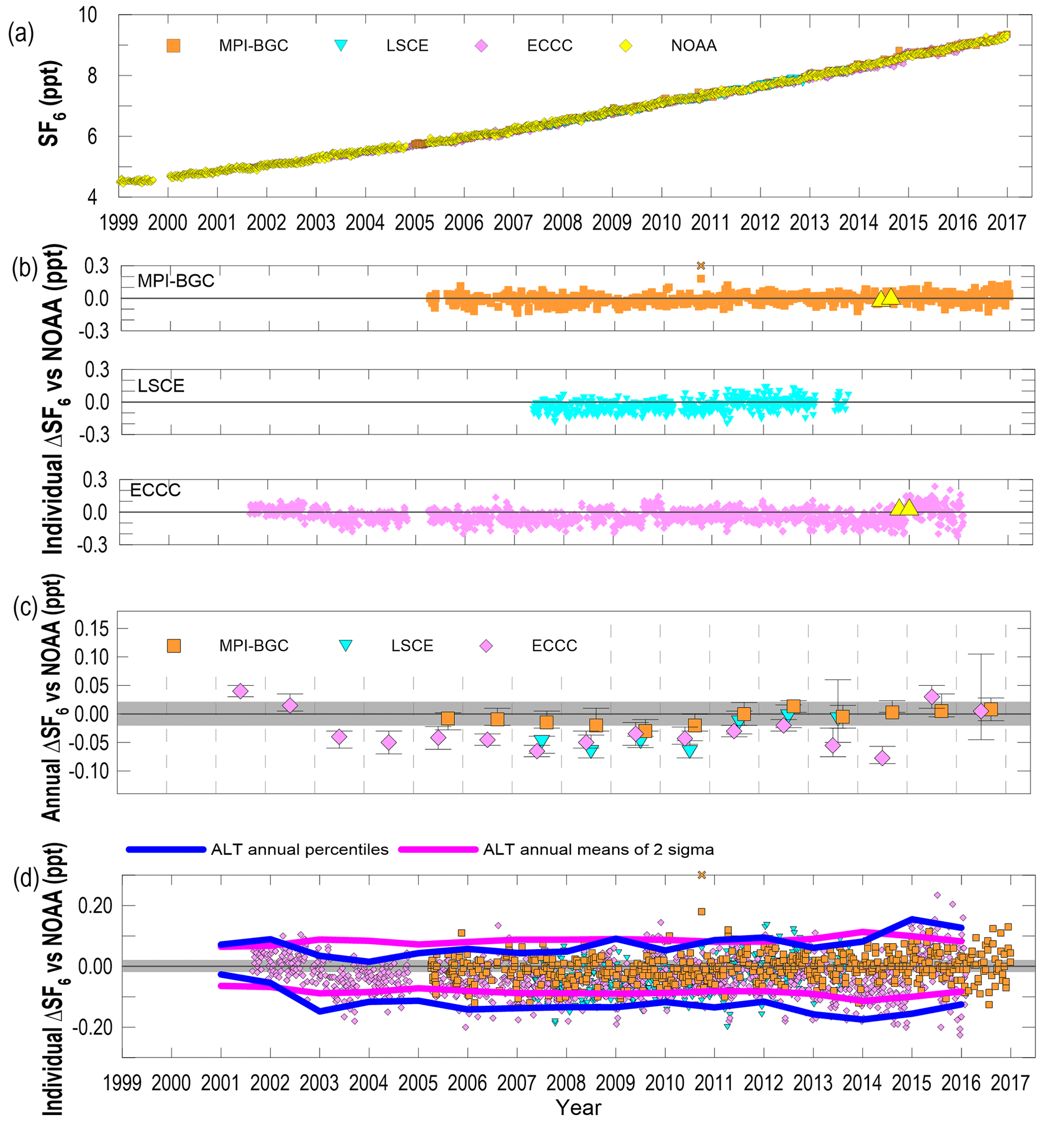
Figure 6 Atmospheric SF₆ comparison results (in ppt) from flask samples taken at ALT by four laboratories (MPI-BGC, LSCE, ECCC, and NOAA). (a) Time series of each laboratory's measurements at ALT, showing long-term trends and seasonal patterns in the records. (b) Individual SF₆ differences (laboratory minus NOAA) at ALT (in ppt). Differences exceeding the y-axis range are plotted with an “X” symbol on the outer axis. Results from the WMO/IAEA Round Robin experiments are overlaid in yellow triangles. The shaded grey band around the zero line indicates the WMO-GAW-recommended measurement agreement goal of ± 0.02 ppt. (c) Annual median SF₆ differences (laboratory minus NOAA) at ALT (in ppt) with the lower and upper limits of estimated 95 % CI. (d) Individual differences (laboratory minus NOAA) at ALT (in ppt) for all the laboratories as a collective. The annual 2.5th and 97.5th percentiles of the entire difference distribution from all laboratories at ALT are shown in blue (−0.14 to +0.09 ppt). The pink lines show the annual means of ± 2σ variations of weekly sampling episodes at ALT (± 0.09 ppt), and there is no MLO data because neither CSIRO nor SIO measures SF₆.

The results from the co-located comparison experiments between CSIRO and NOAA at Mauna Loa (MLO) and at Cape Grim (CGO) (Fig. 5d, Table S25) show the median difference of all individual N₂O measurements to be −0.17 (95 % CI: −0.21, −0.13) ppb at MLO, which is consistent with our findings in Alert of −0.17 (95 % CI: −0.20, −0.13) ppb. At CGO this median difference is −0.03 (95 % CI: −0.06, 0.00) ppb, which is slightly smaller than the ALT and MLO results. Considering the previously mentioned effects of water on the N₂O measurements, the differences could potentially arise from site-specific sampling parameters, such as CSIRO's change to a cryocooler in 2014 at CGO or NOAA's use of a partially dried sample at CGO (although not at MLO or ALT). However, pinpointing the exact cause is beyond the scope of this paper.

Finally, we estimate a measurement agreement for the six independent Alert N₂O data records as a collective, to be within −0.75 to +1.20 ppb (N=3957) over the entire period of 1999–2016 (Table S26). For the approach of using the means of the 2σ variation from weekly sampling events, we estimate a corresponding overall measurement agreement of ± 0.64 ppb (n=801) (pink lines in Fig. 5e). For comparison, we have included the annual means of the combined 2σ variation results of ± 0.64 ppb (n=366) at MLO in yellow lines (Fig. 5e and Table S26).

3.6 SF₆

All measurements are reported relative to the NOAA X2014 SF₆ mole fraction scale (Hall et al., 2011; Lim et al., 2017). Measurements of atmospheric SF₆ are reported in picomoles (trillionths or 10⁻¹² of a mole SF₆) per mole of dry air and abbreviated “ppt” (parts per trillion). All SF₆ measurements from the four laboratories in this study (MPI-BGC, LSCE, ECCC, and NOAA) were determined using GC-ECD analytical methodology. The estimated repeatability of SF₆ measurements, based on replicated injections of standard tank gas, using the dual N₂O/SF₆ GC-ECD system is ∼ 0.04 ppt.

Figure 6a–d and Tables S27–S28 show the corresponding information for SF₆. Please note that there is one less figure and table than the other species, because there are no SF₆ results from the other sites (MLO and CGO), and the last figure and table have been shifted up by one, compared to other species. Table S27 and Fig. 6c show that the MPI-BGC and NOAA SF₆ measurements meet the WMO-recommended ± 0.02 ppt SF₆ compatibility window in 11 of the 12 comparison years (2005–2016). Annual median differences between ECCC and NOAA measurements for 2003–2014 show a constant median offset of −0.05 ppt. The annual differences between LSCE and NOAA measurements for 2007 to 2010 show a similar average offset of approximately −0.05 ppt but showed good agreement from 2011 to 2013. Results from the periodic round robin experiments (Fig. 6b, Table S1) are consistent with the co-located comparison results for each participating laboratory. Again, we find the analysis of median differences by month for each laboratory (not shown) does not indicate any seasonal dependencies.

We find the four independent co-located SF₆ records at Alert (Table S28) are consistent to within a window of −0.14 to +0.09 ppt (N=2359) using 2.5th and 97.5th percentiles and ± 0.09 ppt (N=723) using the mean of the 2σ approach over the time period, respectively. Figure 6d shows individual measurement differences relative to the NOAA reference for all laboratories, the WMO-recommended target range (dark grey band), and our estimate of the overall measurement agreements (in blue and pink lines). There are no SF₆ measurements at MLO or CGO to make general comparisons with the Alert data records.

4 Summary and conclusions

We presented a comparison of measurements of CO₂, CH₄, N₂O, and SF₆ and the stable isotope ratios of CO₂ (δ¹³C, δ¹⁸O) in co-located air samples collected at Alert, Nunavut, Canada, by seven laboratories (ECCC, CSIRO, MPI-BGC, UHEI-IUP, LSCE, SIO, and NOAA (in collaboration with INSTAAR)) spanning 17 years. We also evaluated the consistency of measurements between certain laboratories (CSIRO, SIO, and NOAA/INSTAAR) at three sites (ALT, MLO, and CGO), where other co-located flask sampling programs operate.

From this work, we find that the co-located atmospheric CO₂ and CH₄ measurement records from Alert by CSIRO, MPI-BGC, SIO, UHEI-IUP, ECCC, and NOAA are compatible to the WMO network compatibility goals within ± 0.1 ppm CO₂ and ± 2 ppb CH₄ at the 95 % CI, respectively, over the 17-year period. In addition, we find that the co-located comparison programs at MLO and CGO show similar agreement levels to those at Alert within a range of ± 0.1 ppm for CO₂ between CSIRO, SIO, and NOAA records and within a range of ± 2 ppb for CH₄ between CSIRO and NOAA records. An important caveat to these CO₂ and CH₄ results is that we often observe periods where the biases between datasets exceed the WMO target levels and may persist as a systematic bias for months or years, which could impact our observed compatibility. Our analysis shows that for δ¹³C–CO₂, δ¹⁸O–CO₂, N₂O, and SF₆, our estimate of the overall measurement agreements during the time of this study exceeds the WMO-recommended targets. Differences in the respective local-scale implementations for the isotopes of CO₂, possible moisture effects for δ¹⁸O–CO₂, and the analytical precision of the instruments used for N₂O and SF₆ are possible limiting factors for these results. In addition, the N₂O may have some biases introduced by sample collection procedures.

Further analysis shows that the overall results observed for CSIRO, SIO, and NOAA/INSTAAR's CO₂, CH₄, and δ¹³C–CO₂ for the study period are roughly consistent among the three sites (ALT, MLO, and CGO), implying that merging these records could be done across these specific networks. However, for the δ¹⁸O–CO₂ and N₂O records, future data may be needed to make definitive statements about compatibility across networks.

Although most of the co-located independent CO₂ and CH₄ atmospheric records at Alert meet the WMO-recommended targets when considering the results over the entire study period (1999–2016), meeting the compatibility targets for other trace gas species and stable isotopes in CO₂ continues to be a challenge. The independent measurement records could still be used together for various scientific applications (e.g., long-term trend analysis of CO₂ in Sect. 3.1), even though individual data points are not fully compatible with the WMO-GAW-recommended targets. Furthermore, if we provide data users with the estimated overall measurement agreements for multiple records, they could then take these estimates into account, along with the measurement uncertainties from individual records, while using the datasets for relevant applications.

For each trace gas species and isotope, we have estimated an overall measurement agreement among the Alert records by aggregating all individual differences from each participating laboratory (relative to the NOAA or INSTAAR reference) and then computing the 2.5th and 97.5th percentiles for the entire available periods. This upper and lower limit contains 95 % of the entire difference distribution from all participating laboratories and represents our best estimate of measurement agreement for these data records. The ranges of the estimated overall measurement agreement when combining all individual flask records from Alert over the entire available periods are −0.51 to +0.53 ppm for CO₂, −0.09 ‰ to +0.07 ‰ for δ¹³C–CO₂, −0.50 ‰ to +0.58 ‰ for δ¹⁸O–CO₂, −4.86 to +6.16 ppb for CH₄, −0.75 to +1.20 ppb for N₂O, and −0.14 to +0.09 ppt for SF₆. Using another alternative approach as discussed in Sect. 2.6., we provide the means of the 2σ of each weekly sampling episode, involving all participating laboratories over the entire available time period, which are ± 0.37 ppm for CO₂, ± 0.06 ‰ for δ¹³C–CO₂, ± 0.31 ‰ for δ¹⁸O–CO₂, ± 3.62 ppb for CH₄, ± 0.64 ppb for N₂O, and ± 0.09 ppt for SF₆. Results from this analysis reveal overall cumulative differences due to errors introduced at one or more steps in the entire atmospheric measurement process, including sampling and analytical procedures.

In summary, this study assesses the level of measurement agreement among individual programs by comparing co-located flask air measurements. It enhances confidence in the uncertainty estimation while using those datasets either individually or collectively across diverse applications. Conducting such comprehensive analysis regularly is advisable to detect potential issues and monitor any scale and/or instrumentation changes. It is recommended that future analyses be carried out every 2 years by a dedicated entity and be reported regularly during WMO/IAEA GGMT meetings.