Identification of spikes in continuous ground-based in situ time series of CO₂, CH₄ and CO: an extended experiment within the European ICOS Atmosphere network

The identification of spikes (i.e., short and high variability in the measured signals due to very local emissions occurring in the proximity of a measurement site) is of interest when using continuous measurements of atmospheric greenhouse gases (GHGs) in different applications like the determination of long-term trends and/or spatial gradients, inversion experiments devoted to the top-down quantification of GHG surface–atmosphere fluxes, the characterization of local emissions, or the quality control of GHG measurements. In this work, we analyzed the results provided by two automatic spike identification methods (i.e., the standard deviation of the background (SD) and the robust extraction of baseline signal (REBS)) for a 2-year dataset of 1 min in situ observations of CO₂, CH₄ and CO at 10 different atmospheric sites spanning different environmental conditions (remote, continental, urban).

The sensitivity of the spike detection frequency and its impact on the averaged mole fractions on method parameters was investigated. Results for both methods were compared and evaluated against manual identification by the site principal investigators (PIs).

The study showed that, for CO₂ and CH₄, REBS identified a larger number of spikes than SD and it was less “site-sensitive” than SD. This led to a larger impact of REBS on the time-averaged values of the observed mole fractions for CO₂ and CH₄. Further, it could be shown that it is challenging to identify one common algorithm/configuration for all the considered sites: method-dependent and setting-dependent differences in the spike detection were observed as a function of the sites, case studies and considered atmospheric species. Neither SD nor REBS appeared to provide a perfect identification of the spike events. The REBS tendency to over-detect the spike occurrence shows limitations when adopting REBS as an operational method to perform automatic spike detection. REBS should be used only for specific sites, mostly affected by frequent very nearby local emissions. SD appeared to be more selective in identifying spike events, and the temporal variabilities in CO₂, CH₄ and CO were more consistent with those of the original datasets. Further activities are needed for better consolidating the fitness for purpose of the two proposed methods and to compare them with other spike detection techniques.

1 Introduction

High-precision continuous measurements are needed to monitor the long-term variability in well-mixed greenhouse gases (GHGs) in the atmosphere, which are responsible for a large fraction of the anthropogenic forcing to the climate system (IPCC, 2021). These observations are needed to attribute, quantify and reduce uncertainties about the role of the Earth's surface–atmosphere fluxes in determining long-term changes as well as to investigate the complex interactions between GHG fluxes and climate variability (Byrne, 2020). Atmospheric observations can be effectively used in inversion model systems to obtain optimized information of the spatial and temporal variations in the net atmospheric fluxes over local, regional and global scales (e.g., Christen, 2014; Palmer et al., 2018; Friedlingstein et al., 2022). For such applications, it is pivotal to operate measurement networks whose surface footprints are representative enough of the tagged spatial regions. However single sites should be rarely subject to influences of very local emissions that represent confounding signals for the correct evaluation of regional and global fluxes. Moreover, accurate measurements are required at the measurement sites (in terms of calibration scales) with high precision and sufficient time resolution.

In the framework of the Integrated Carbon Observation System research infrastructure (ICOS RI) (Heiskanen et al., 2022), a pan-European monitoring network providing highly compatible, harmonized and high-precision scientific data on the carbon cycle and greenhouse gases was established. ICOS RI is organized across three domains (atmosphere, ecosystems and oceans): the atmospheric network provides continuous in situ data of carbon dioxide (CO₂), methane (CH₄) and carbon monoxide (CO) besides other GHGs (i.e., N₂O) and atmospheric variables relevant for the investigation of the European carbon cycle. Since the aim of the ICOS RI atmospheric network is to be compliant with the World Meteorological Organization (WMO) network compatibility goals (WMO, 2020), the measurements are performed following common guidelines and requirements (ICOS RI, 2020). Also the data treatment follows standardized and centralized procedures: all raw data recorded by the measurement sites are delivered in near real time (i.e., with a 24 h delay) to the ICOS Atmospheric Thematic Centre (ATC) for the application of automatic quality checks, averaging to 1 min and 1 h mean values (Hazan et al., 2016), and the release of the ICOS Near Real-Time data collection (ICOS RI, 2018). Manual revision of the data is performed by the site principal investigator (PI) using a common quality assurance/quality check application (ATC QC) running at the ATC server. After this quality control step and a final common review within the ICOS Atmosphere Monitoring Station Assembly, a fully quality controlled Level-2 dataset is released (ICOS RI, 2022). Common instructions about data validation were defined within ICOS, and data have to be invalidated by the site PI only for objective and testified reasons (such as instrument failures or contamination due to maintenance works).

Very local emissions that might occasionally occur in the proximity of the measurement sites and that can produce short but intense variability in the measured GHG signals (i.e., spikes) can jeopardize the full value of these atmospheric measurements when, e.g., using those to constrain the quantification of GHG atmospheric fluxes at regional and global scales. Here, “local” refers to emissions occurring in a range of a few kilometers (i.e., ∼ 10 km) from the site which cause positive short-term spikes with a maximum duration from minutes to less than a few hours. These signals are not suitable for investigating regional-scale (∼ 100–500 km) fluxes within the site surface sensitivity area (Oney et al., 2015; Storm et al., 2023) because they are superimposed onto the GHG variability resulting from the atmospheric background and the regional signal. As an example, the observation records affected by the influence of nearby emission sources should be filtered out for their use in regional or global inversion experiments (e.g., Bergamaschi et al., 2022). According to the ICOS flagging instructions, these very local contamination events (engine exhaust, local construction, fires, cars, etc.) must be considered valid but with a specific descriptive flag (“non-background conditions”).

In this work, we considered two automatic spike identification methods: the standard deviation of the background (SD) and the robust extraction of baseline signal (REBS) methods. They were already tested in a previous study (El Yazidi et al., 2018): based on this earlier investigation, the SD method was selected to be operationally implemented in the ICOS Atmosphere data processing chain to provide an experimental identification of spike occurrence at the measurement sites (see https://icos-atc.lsce.ipsl.fr/P0030.1, last access: 9 October 2023). A recent expansion of the ICOS atmospheric network represented an opportunity to test the two methods on a wider number of sites and over more extended time frames. The motivation to evaluate the ability of automatic spike identification methods was mainly threefold. Firstly, there is a strong need for some data users to exclude spikes from their analysis as already mentioned above. For example, inversion experiments devoted to the top-down quantification of GHG emissions need to use de-spiked records of atmospheric observations because very local processes can be neither resolved by the models nor appropriately represented in the emission inventories. Secondly, the identification of local spikes can be useful for the analysis and the characterization of specific local emissions. For instance, by analyzing the spike related to emissions from nearby ship transits, Grönholm et al. (2021) used CO₂, CH₄ and CO data from the ICOS Utö site (Finland) to provide an improved characterization of the emission ratios of ships powered with liquified natural gas (LNG). Thirdly, a reliable and effective automatic spike methodology represents a powerful tool in the hands of site PIs when performing routine data quality control. Recently, Hoheisel et al. (2023) and Affolter et al. (2021) analyzed the spike occurrences at high mountain sites to infer the impact of local contamination related to local human activities (tourism, construction works) on long-term atmospheric measurements of CO₂ and CH₄.

The present study aimed at investigating the sensitivity of the spike identification in continuous (1 min time resolution) observations of CO₂, CH₄ and CO as a function of different settings of the two tested methods as well as at assessing and documenting the impact of these de-spiking procedures at different temporal aggregations (i.e., hourly, monthly and seasonal averages). Finally, we assessed the effectiveness of the two automatic methods in detecting spikes by investigating case studies and comparing the automatic de-spiking results with those provided by manual spike identification. To do so, CO₂, CH₄ and CO observations carried out at 10 atmospheric sites representative of different environmental conditions (remote, continental, urban) were considered.

2 Experiment and methods

2.1 Measurements sites

Subsets of data from remote sites (Utö, Jungfraujoch, Zugspitze, Pic du Midi and Monte Cimone), continental sites (Karlsruhe, Saclay, Ispra), one semi-urban site (Pujo) and one urban site (Paris Jussieu) were used to assess the performance of the spike identification methods in different environmental conditions (Table 1). With the term “remote”, we considered sites which are less directly and less frequently exposed to strong anthropogenic emissions. “Continental” indicates stations targeting predominantly continental air masses, while “urban” indicates stations located in metropolitan districts. In this paper, we adopted this site classification because we expected different occurrences of spikes as a function of the more or less direct exposure to anthropogenic emissions. Since several sites sample from different heights above ground and, thus, record multiple time series, 19 different combinations of sites and heights were investigated for CO₂ and CH₄ and 16 for CO (as there were no CO measurements at Puijo (PUI) during the inspected time period).

Table 1 List of specific instruments working at the considered test sites during the study period. Sites are listed in alphabetical order according to their classifications (remote, non-remote). ICOS-labeled sites are identified by an asterisk.

2.1.1 Utö – Baltic Sea (UTO, Finland)

The UTO site (59.78^∘ N, 21.37^∘ E) is located on the island of Utö on the outskirts of the Archipelago Sea in the Baltic Sea about 80 km southwest from mainland Finland. The island is about 1 km² in size, mostly rocky and treeless. Typical vegetation is low and consists of grass and shrubs. The main part of the Baltic Sea is to the south (500 km); the Gulf of Finland is to the east (400 km). The ICOS measurements are carried from a cell phone mast at 57 m a.g.l. and 65 m a.s.l., about 200 m from the coast (Grönholm et al., 2021).

The population on the island is ∼ 50 people. Local emissions include mainly small boats and a ferry to the mainland, which may stay overnight in the harbor. Ahvenanmaa (alternately Åland), an autonomous region of Finland, is to the northwest at a distance of 70–120 km. The regional capital city Mariehamn (11 500 inhabitants) is located 90 km from UTO. Turku (186 000 inhabitants) is 90 km away to the NE. Stockholm is 200 km to the W–SW.

2.1.2 Jungfraujoch (JFJ, Switzerland)

This high alpine site (46.55^∘ N, 7.98^∘ E; 3580 m a.s.l.) is situated on a mountain saddle between the two mountains Jungfrau (4158 m a.s.l) and Mönch (4099 m a.s.l.). The local wind is channeled due to the topography. Surrounding surfaces are mostly covered by snow or ice apart from some steep slopes of bare rock. No vegetation or soil is present in the vicinity.

The central laboratory for atmospheric observations is located in the uppermost building of the Jungfraujoch facilities, the so-called Sphinx Observatory, which was established in 1937 (Balsiger and Flückiger, 2016). The Sphinx Observatory is also accessible for tourists, with a public terrace approximately 10 m below the inlet (which is on the top), while the upper part (three floors) is restricted to scientists. According to Affolter et al. (2021), about 1 million tourists visit the Jungfraujoch per year. The closest settlements are the tourist villages Wengen (1200 inhabitants) and Grindelwald (3800 inhabitants), approximately 8 km to the NW and 10 km to the NE, respectively. Both are located about 2500 m below Jungfraujoch. Interlaken (5700 inhabitants) is located approx. 3 km below Jungfraujoch and 20 km to the north. Thun (42 600 inhabitants) and Bern (140 000 inhabitants) are located approximately 35 and 60 km to the NW. The Po basin in northern Italy is located ∼ 150 km to the SE. The impact of regional contributions to the CO₂ signal at Jungfraujoch was recently assessed by Pieber et al. (2022).

2.1.3 Zugspitze (ZSF, Germany)

Mt. Zugspitze is the highest mountain of the German Alps. It is located in southern Germany, about 90 km SW of Munich, at the Austrian border near the town of Garmisch-Partenkirchen. The environmental research station “Schneefernerhaus” (47.42^∘ N, 10.79^∘ E; 2666 m a.s.l.), where the ICOS measurements are carried out (Hoheisel et al., 2023), is located on the southern slope of Mt. Zugspitze. There is no vegetation on the site, and the terrain is bare rocks, covered by snow from October to June. The nearest villages and towns are Ehrwald–Lermoos (6 km away, 2600 inhabitants, 1000 m a.s.l.), Grainau (7 km, 3500 inhabitants, 750 m a.s.l.) and Garmisch-Partenkirchen (12 km, 29 000 inhabitants, 708 m a.s.l.). The nearest largest urban areas are Innsbruck (38 km, 133 000 inhabitants, 574 m a.s.l.) and Munich (92 km, 1 558 000 inhabitants, 519 m a.s.l.). Please note that for ZSF only data during 2021 were used in this experiment.

2.1.4 Monte Cimone (CMN, Italy)

The CMN site (44.19^∘ N, 10.70^∘ E) is located at the top of Mt. Cimone (2165 m a.s.l.), the highest peak of the northern Apennines, and it is characterized by a 360^∘ free horizon. The ICOS site is hosted at the “O. Vittori” Observatory (Cristofanelli et al., 2018), which is located above the timberline: only some patches of grass can be found on the mountaintop, which is mostly rocky and covered with snow for 6–7 months a year. CMN overlooks the highly industrialized Po basin (towards the NW–SE) and northern Tuscany (towards the S–NW). The most important urban areas are Modena (185 000 inhabitants, 50 km to the N), Bologna (390 000 inhabitants, 60 km to the NE) and Florence (380 000 inhabitants, 55 km to the SE). Local emission sources can be represented by tractors used for transporting items to the mountaintop, helicopters and diesel engines used as emergency power supply at the nearby Italian Air Force observatory. During summer, tourists (roughly 500–600 persons yr⁻¹ for the July–August period) can access the terrace of the “O. Vittori” Observatory (approximately 5 m below the sampling inlet).

2.1.5 Pic du Midi (PDM, France)

This high mountain site (42.56^∘ N, 0.80^∘ E) is located on the NW side of the Pyrenees in the SW of France. Due to the high elevation (2877 m a.s.l.), PDM is affected by air masses from the free troposphere from the Atlantic Ocean. Like other mountain sites, PDM can be affected by upslope winds and valley wind circulations especially in summer and early autumn, bringing air from the boundary layer of southwest France (covered by intensive croplands and forests, e.g., Fu et al., 2016). In 2015, a field campaign was carried out at PDM to investigate the impact of a small sewage treatment facility on the atmospheric CH₄ observations (El Yazidi et al., 2018). The same dataset was considered in this work to assess the efficacy of the automatic spike detection methods (Sects. 3.4 and 3.6).

2.1.6 Ispra (IPR, Italy)

This site (45.81^∘ N, 8.64^∘ E) is located at the southeastern border of Lake Maggiore in a semi-rural area at the NW edge of the Po Valley at a distance of 60–100 km from the alpine mountains.

The ICOS site is located within the premises of the Joint Research Centre, Ispra (Putaud et al., 2021), at the border of the village of Ispra (5300 inhabitants). Local emission sources are represented by two cement factories (8.4 km to the NNE and 5.1 km to the SE). Moreover, in the vicinity of the station, agricultural activities from livestock farming can impact the CH₄ measurements and in the case of stagnant weather conditions (with wind speeds $<\sim \mathrm{1}$ m s⁻¹) can create spikes exceeding a few parts per million (Bergamaschi et al., 2022). IPR is equipped with a tall concrete tower (100 m high) with three sampling levels (40 m, 60 m, 100 m a.g.l.).

2.1.7 Jussieu Paris (JUS, France)

The JUS site (48.85^∘ N, 2,36^∘ E) is an urban station located in the center of Paris (5th arrondissement), on a university campus that houses about 40 000 students and staff. The central area of Paris extends to 105 km² and has 2 million inhabitants, while the Paris agglomeration has 11 million. The air inlet is located on the roof of the main building (30 m a.g.l.) on one side of a small concrete structure present on the roof. The campus roofs are part of an experimental research platform dedicated to the observation of the chemical and dynamic variabilities in the lower atmosphere and therefore house scientific equipment; they are accessible by technical staff. The surroundings include the Seine River, which passes to the NE of the campus, and the Jardin des Plantes, a park and botanical garden with an area of 27 ha, to the SE. To the W, the Zamansky Tower is the tallest building on campus (90 m a.g.l.), but the rest of the campus as well as the rooftops of Paris is at an elevation of 25–30 m a.g.l.

2.1.8 Karlsruhe Observatory (KIT, Germany)

The KIT site (49.09^∘ N, 8.42^∘ E) is located in a semi-rural region in the Upper Rhine Valley at Campus North of the Karlsruhe Institute of Technology, 12 km north of the city of Karlsruhe (300 000 inhabitants) and near Eggenstein-Leopoldshafen (2 km W, 15 000 inhabitants). Other smaller towns in the surroundings (< 15 km) are Wörth (∼ 17 600 inhabitants), Linkenheim-Hochstetten (12 000 inhabitants), Stutensee (24 000 inhabitants), Bruchsal (44 000 inhabitants) and Graben-Neudorf (11 500 inhabitants). At the measurement site, the Rhine Valley is about 40 km wide and surrounded by 300–400 m hills on both sides. The land use in this area is dominated by agricultural fields (ca. 50 %); forests and green areas cover about 11 % and villages and traffic about 17 %. Local point sources in the near-distance range (< 20 km) are a coal power plant, an oil refinery, two paper mills and one cement factory (E-PRTR, 2017). The site is equipped by a tall tower with four sampling levels (30 m, 60 m, 100 m, 200 m a.g.l.) (Kohler et al., 2018).

2.1.9 Puijo (PUI, Finland)

The PUI site (62.91^∘ N, 27.65^∘ E) is located in the city of Kuopio, on top of a 75 m observation and radio transmittance tower. The tower stands on a hill, and its base is 149 m above the surrounding lake level, which is 82 m a.s.l. Two sampling inlets are available: on top of a 10 m mast on the roof of the tower (84 m a.g.l.) and at 47 m a.g.l. The measurement site is located at the southern boreal climatic zone, which is characterized by forests with conifer (mostly pine and spruce) and deciduous (mostly birch) trees, an undulating terrain with rocky soil and moderate height hills, and lots of long lakes in the NW–SE direction.

Nearby sources at PUI are represented by the Puijo tower (restaurant and sewerage ventilation, ∼ 10 m below the top inlet, ∼ 27 m above the lower inlet), a district heating plant 3.5 km to the SE (∼ 114 m below the top inlet, ∼ 77 m below the lower inlet), a paper mill 5 km to the NE (∼ 164 and ∼ 127 m below the inlets), a highway in the N–S direction (∼ 230 and 193 m below the inlets) and a waste disposal site 10.5 km to the SW. The Puijo tower is also accessible to tourists (roughly 100 000 persons yr⁻¹, during the high season of June–August on average 800 persons d⁻¹) and has a viewing platform at ∼ 15 m below the top inlet and ∼ 22 m above the lower inlet.

2.1.10 Saclay (SAC, France)

The SAC site (48.72^∘ N, 2.14^∘ E) (Lian et al., 2021) is a semi-urban site. This site is surrounded by agricultural fields (47.4 %), forests (25.0 %), and urban residential areas (22.2 %). The site is located ∼ 20 km SW of the center of Paris on the Plateau de Saclay. The closest village and small town are Saint-Aubin (700 inhabitants) and Gif-sur-Yvette (approx. 21 400 inhabitants), located 500 m NW and 1 km to the S of the station, respectively. There is a busy road (N118) located 1 km from the site. SAC is equipped with a tall tower (100 m high) with three sampling levels (15 m, 50 m and 100 m a.g.l.), equipped with meteorological sensors.

2.2 Measurement methods

Within the ICOS atmospheric network, the sampling equipment setup, sampling procedures, calibration strategy and data processing are executed according to highly standardized and well-documented procedures (ICOS RI, 2020). In particular, as reported by Yver Kwok et al. (2015), the instruments providing CO₂, CH₄ and CO data must be tested at the ICOS Atmospheric Thematic Centre (ATC) Metrology Laboratory (MLab) before their use in the network. The list of accepted analyzers is regularly updated to keep up with new technologies that are continuously tested at ATC. According to ICOS RI (2020), all sampling heights at tall towers (e.g., PUI, IPR, KIT and SAC) should be sampled sequentially within an hour in order to retrieve hourly vertical gradients. This means that for tall towers, for each single sampling height, fewer than sixty 1 min records are available for each hour. The switching sampling strategy is slightly different for each measurement site, but since the highest site is considered the most important (for obtaining regional signals suitable for modeling purposes), priority is usually given to the sampling from the uppermost height. Thus, observations from the highest inlet have the largest data coverage within each single hour. CO₂, CH₄ and CO are measured at all the considered sites except for PUI, where only CO₂ and CH₄ were measured during the considered period. The considered time series spanned the period 2019–2020. Exceptions were ZSF, for which the year 2021 was considered (due to the fact that ZSF joined ICOS in 2021), and PDM, for which data from the 2015 field campaign (El Yazidi et al., 2018) were analyzed. The specific GHG analyzers used at each considered measurement site are reported in Table 1.

2.3 Spike detection methods

The SD and REBS methods were applied to the 1 min datasets of the sites considered in this experiment. These data are generated in intermediate steps within the data processing for the creation of the Level-2 final dataset (Hazan et al., 2016).

2.3.1 Standard deviation of the background (SD)

As reported by El Yazidi et al. (2018), the SD method is designed to select the first available data point, which is assumed not to be a spike (C_nospike). Then, the next data point (C_i) in the time series of 1 min data is evaluated with respect to C_nospike: spikes are identified when C_i is higher than a threshold defined as

$$\begin{array}{}\text{(1)}& C_{\mathrm{nospike}}+\mathit{\alpha }\times \mathit{\sigma }+\sqrt{n}\times \mathit{\sigma }.\end{array}$$

If C_i is lower than the threshold from Eq. (1), it is considered “non-spike” and becomes the new reference value. The method was applied to the 1 min data with two modes, forwards and backwards: all the detected spikes are kept.

In Eq. (1), α is the parameter to control the selection threshold, n is the number of data between C_nospike and C_i, and the parameter σ is the standard deviation of data falling between the first and the third quartile of the data distribution obtained by considering a 240 h time window before C_nospike. The default values of α (1 for CO₂ and CH₄ and 3 for CO) were based on the results provided by El Yazidi et al. (2018) and are currently implemented in the operational spike detection chain in use for the whole ICOS Atmosphere network. The sensitivity analyses presented in this work (Sect. 3.1) considered $\mathit{\alpha }=\mathit{\{}\mathrm{0.1},\mathrm{1},\mathrm{4}\mathit{\}}$ for CO₂ and CH₄ and $\mathit{\alpha }=\mathit{\{}\mathrm{0.1},\mathrm{3},\mathrm{4}\mathit{\}}$ for CO. In general, larger α values tend to reduce the sensitivity of the algorithm towards spike detection. As the spike detection methods were applied per sampling height, a minimum number of valid 1 min data was defined for allowing an effective application. Based on the tests done by El Yazidi et al. (2018), a minimum of 4 full contiguous days (5760 min) should be available for the application of SD for a site with only one sampling height (e.g., CMN, JFJ, ZSF, UTO, JUS). This threshold was decreased to 3000 min for a site with two sampling heights (e.g., PUI), to 2400 min for a site with three sampling heights (e.g., IPR, SAC) and to 1400 min for a site with four sampling heights (e.g., KIT).

2.3.2 Robust extraction of baseline signal (REBS)

The REBS method (Ruckstuhl et al., 2001, 2012) is a statistical method based on a local linear regression of the time series over a moving time window (characterized by a duration called the “bandwidth”), to account for the slow variability in the baseline signal, with outliers lying above the modeled baseline iteratively discarded. The REBS code run by ATC is based on the rfbaseline application developed in the IDPmisc package (Locher, 2020) for the R environment. Because the targeted spikes last a few minutes to a few hours, a bandwidth of 60 min was implemented.

The detection of spikes by REBS is based on the calculation of the following threshold:

$$\begin{array}{}\text{(2)}& \widehat{g}\left(t_i\right)+\mathit{\beta }\times \mathit{\gamma }.\end{array}$$

A data point C_i which exceeded this threshold value was considered a spike. In Eq. (2), β is a tuning parameter (for details, see Ruckstuhl et al., 2012). By default, β is set to 3 for CO₂ and CH₄ and 8 for CO. γ is a scale parameter that represents the standard deviation of data below the baseline curve $\widehat{g}\left(t_i\right)$, which, for this experiment, was calculated by the R rfbaseline function (2020) over the previous 24 h of data. The sensitivity analyses presented in this work (Sect. 3.1) inspected the impact of changing β values with $\mathit{\beta }=\mathit{\{}\mathrm{1},\mathrm{3},\mathrm{10}\mathit{\}}$ for CO₂ and CH₄ and $\mathit{\beta }=\mathit{\{}\mathrm{1},\mathrm{8},\mathrm{10}\mathit{\}}$ for CO. Larger β values tend to reduce the sensitivity towards spike detection. Similarly to the SD approach, a minimum number of valid minute data was set for the method application based on the number of sampling heights at each site. For the application of REBS, one-third of the data recorded within a day (524 min) were requested to be available for a site with a single sampling height. This value decreased to 273 min for a site with two sampling heights, to 218 min for a site with three sampling heights and to 127 min for a site with four sampling heights.

3 Results

3.1 Sensitivity of spike detection to the setting parameters

To provide an overview of the impact of the algorithm settings on the number of observations identified as spikes, we calculated the percentage of the data selected on the 1 min dataset for the different sites, methods and setting parameters (see Figs. 1–3). To this aim, the two methods were run with the three different configurations reported in Sect. 2.3.

Figure 1 Percentages of the 1 min CO₂ data selected as spikes by SD (a) and REBS (b) over the period 2018–2020 (for ZSF_880_h3^*, only 2021 was considered), for the different algorithm settings. For SD, α was set to 0.1 (SD0.1), 1.0 (SD1.0) and 4.0 (SD4.0). For REBS, α was set to 1 (REBS1), 3 (REBS3) and 10 (REBS10). The codes reported as labels for the x axis indicate the combination of site, instrument(s) ID and sampling height (m a.g.l.).

Figure 2 The same as Fig. 1 but for CH₄.

Figure 3 The same as Fig. 1 but for CO.

3.1.1 Carbon dioxide (CO₂)

By considering the application of the SD algorithm with the “standard” ATC setting (i.e., α=1.0), the averaged percentage of 1 min CO₂ data considered spikes was mostly below 1 % for all the sites and sampling heights: values exceeding 2 % were observed for the highest level of KIT and PUI (Fig. 1). By adopting α=0.1, the number of detected spikes increased by factors of 2 to 4 as a function of the sites: the most evident changes were observed for CMN, IPR and JUS. By adopting α=4.0, a decrease in the detected spikes occurred in comparison with the standard setting ($\mathrm{16}/\mathrm{18}$ time series reported an averaged spike fraction lower than 0.5 %). For continental sites, a positive tendency was detected for an increase in the number of spikes as a function of sampling heights: as an example, at KIT a 0.5 % spike occurrence was detected at 30 m, which increased to 2.4 % at 200 m for the standard setting. Generally, the highest spike occurrences were detected for the highest sampling height at the continental sites.

By considering the application of the REBS algorithm with the standard ATC setting (i.e., β=3), the averaged percentage of 1 min CO₂ spikes was above 9 % for all the sites and sampling heights (Fig. 1). By adopting β=1, the number of detected spikes increased by factors from 3 to 7 as a function of the sites: the most evident changes were observed for CMN and JUS. By adopting β=10, a decrease in the detected spikes occurred in comparison with the standard setting with $\mathrm{16}/\mathrm{18}$ time series reporting an averaged spike fraction lower than 0.5 %. To evaluate how much the fraction of the detected spikes varied as a function of the different sampling locations, we calculated the ratio of the standard deviation (σ) to the mean values (m) of the averaged spike fraction among the time series. A lower sensitivity to the spike frequency was detected for REBS compared to SD: for the standard settings, the ratio $\mathit{\sigma }/m$ was 0.23 for REBS, while it was 0.80 for SD.

3.1.2 Methane (CH₄)

By considering the application of the SD algorithm with the standard ATC setting (i.e., α=1.0), the averaged percentage of 1 min CH₄ spikes was mostly below 2 % for all the sites and sampling heights: a frequency exceeding 3 % was only observed at IPR (Fig. 2). By adopting α=0.1, the number of detected spikes increased by factors from 2 to 4 as a function of the different sites: the most evident changes were observed for JFJ, JUS, UTO and ZSF. By adopting α=4.0, a decrease in the detected spikes occurred in comparison with the standard setting with $\mathrm{13}/\mathrm{18}$ time series reporting an averaged spike fraction lower than 0.5 %. Generally, the highest spike occurrences were detected for the lowest sampling heights at the continental sites (for instance at IPR, for the standard setting, a 5.0 % spike occurrence was detected at 40 m, which decreased to 3.6 % at 100 m).

By considering the application of REBS with the standard ATC setting (i.e., β=3.0), the averaged percentage of 1 min CH₄ spikes ranged from 6.6 % at ZSF to 22 % at IPR (40 m); see Fig. 2. By adopting β=1, the number of detected spikes increased by factors from 2 to 9 as a function of the locations and sampling heights: the most evident changes were observed for UTO and ZSF. By adopting β=10, a decrease in the detected spikes occurred in comparison with the standard setting with $\mathrm{10}/\mathrm{18}$ time series reporting an averaged spike fraction lower than 0.5 %. Like for CO₂, in respect to SD a lower sensitivity of the spike detection was detected for REBS as a function of the sampling site: for the standard settings, the ratio $\mathit{\sigma }/m$ was 0.32 for REBS with respect to 1.0 for SD.

3.1.3 Carbon monoxide (CO)

By considering the application of the SD algorithm with the standard ATC setting (i.e., α=3.0), the averaged percentage of 1 min CO spikes was below 0.5 % for all the sites and sampling heights (Fig. 3). By adopting α=0.1, the number of detected spikes increased by factors from 3 to 44 as a function of the sites: the most evident changes were observed for the remote sites (CMN, JFJ and UTO) and JUS for which the fraction of detected spikes increased more than 20-fold. By adopting α=4.0, all the sites showed a fraction of spike lower than 0.2 %. No clear tendencies were detected for the dependence of the spike detection on the sampling heights.

By considering the application of the REBS algorithm with the standard ATC setting (i.e., β=8), the averaged percentage of 1 min CO spikes ranged from 0.1 % at CMN to 1.2 % at IPR (40 m); see Fig. 3. By adopting β=1, the fraction of detected spikes largely increased (from 51 % at KIT to 71 % at IPR and UTO). By adopting β=10, the number of detected spikes decreased by ≈ 50 % in respect to the standard setting. For the standard setting, a weak decreasing tendency for the number of spikes was observed by increasing sampling heights (e.g., at IPR the fraction of detected spikes decreased from 1.2 % at 40 m to 0.7 % at 100 m). The opposite was observed when β=1 was considered with the highest sampling levels of the continental sites reporting a [+5 %, +10 %] increase in spike detections in respect to the lowest levels. Despite CO₂ and CH₄, the site dependence of the spike fractions was comparable between SD and REBS.

3.2 Impact of the spike detections on hourly mean values

Because ICOS atmospheric data are typically provided to external users as hourly mean values, it was important to document how the application of the two de-spiking methods impacted the dataset of hourly mean values generated by the temporal aggregation of the 1 min data. To investigate the potential impact of the de-spiking methods on the 1 h average values of CO₂, CH₄ and CO, we calculated the changes in the percentiles of the original data distribution after the application of the de-spiking methods with the standard settings (Fig. 4). For this analysis, only the data record for the highest sampling level was considered for IPR, KIT, PUI and SAC. Specifically, we calculated the arithmetic differences between the data distribution percentiles (5th, 10th, 50th, 90th and 95th) obtained for the de-spiked and the original dataset (i.e., positive values denoted an increase in the percentile value after the application of de-spiking methods). When the application of SD (α = 1.0) is considered for CO₂, impacts on the percentile values were observed for IPR, KIT, PUI and SAC (Fig. 4). For IPR (and somewhat for PUI), the positive differences for the lowest percentile and the negative differences for the higher percentiles implied a narrowing of the data distribution after de-spiking. For KIT and SAC, negative differences were observed over almost all the range of the considered percentiles, thus implying a shift in the data distribution towards lower values. The same tendencies were observed when REBS (β=3) was considered but with a higher impact on the percentile change for IPR. Similar results were found for CH₄: again, impacts of the de-spiking were observed for IPR, KIT, PUI and SAC. However, despite the CO₂ case, a narrowing of the data distribution after de-spiking was evident for all these sites (but KIT). When REBS was used, a wider impact was observed among the stations. Besides IPR, KIT, PUI and SAC, decreases in the upper percentiles were also observed for the remote sites CMN and PDM. A more limited impact was found for CO: for both SD (α=3.0) and REBS (β=8), a narrowing of the data distribution was observed at IPR, SAC and KIT after de-spiking application.

Figure 4 For the different sites (color-coded) the differences in the percentiles of hourly mean values between de-spiked and original dataset for the different species and methods are reported. The horizontal dotted lines represent the WMO network compatibility goal.

3.3 Impact of the spike detections on averaged monthly values

An important point was to investigate the effect of the de-spiking methods on the monthly mean values of CO₂, CH₄ and CO, which are often used to illustrate/determine the long-term variability in and trends of these trace gases. To reach this goal, for each available time series, the differences in the monthly mean values between the de-spiked and the original dataset were calculated for each algorithm and for each setting (i.e., varying α and β values). When referring to the mole fractions, hereinafter, we used the terms “impact” or “significant” when the differences between de-spiked and original dataset exceeded the WMO network compatibility goals (i.e., ±0.1 ppm for CO₂, ±2 ppb for CH₄ and CO; see World Meteorological Organization, 2020).

In general, the impact of de-spiking methods and settings on the monthly mean values depends on the site characteristics (remote vs. continental), on the considered trace gas and on the sampling height. Figures 5 to 7 show the boxplot of the differences (ΔCO₂, ΔCH₄ and ΔCO) between the de-spiked and the original monthly mean values. For CO₂, the SD method (with α={0.1, 1.0}) showed impacts only at KIT and PUI. On the other hand, for REBS, impacts were evident for all the continental sites and for remote sites (in this latter case mostly when β=1 was adopted); only for β=10 were no impacts diagnosed. For CH₄, SD showed impacts only at IPR (for all the adopted settings). Similarly to CO₂, REBS showed impacts at all the continental sites when β={1, 3} was considered. For remote sites, an impact was diagnosed only for CMN with β=1. For CO, significant deviations in respect to the original dataset were observed only for REBS with β=1.

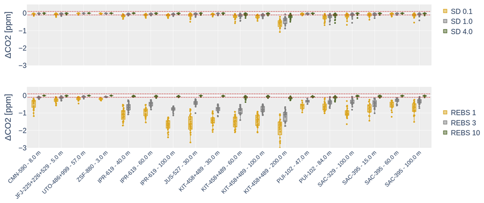
Figure 5 Boxplot differences (ΔCO₂) of the monthly mean CO₂ values between the de-spiked and original dataset. The horizontal red lines represent the ±0.1 ppm WMO network compatibility goal. Each box represents the distribution of the differences for a combination of site and sampling height. The color code indicates, for each algorithm, the adopted setting.

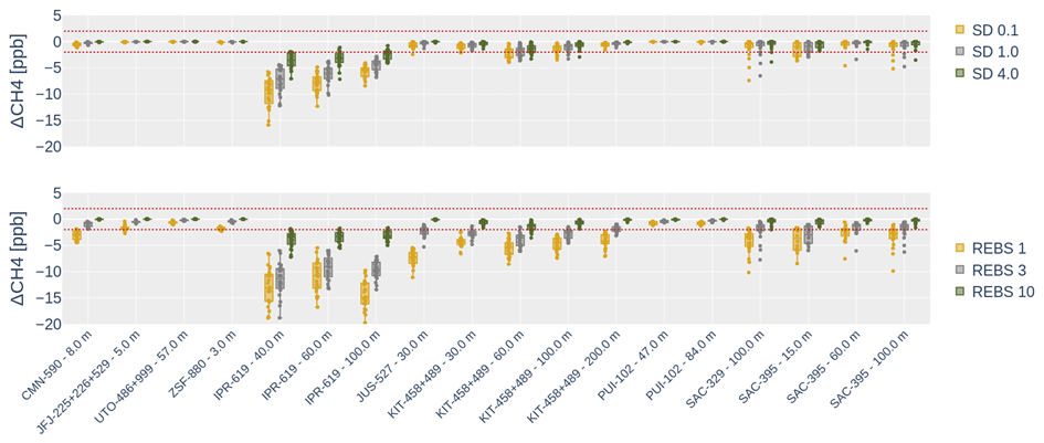
Figure 6 The same as Fig. 5 but for CH₄. The horizontal red lines represent the ±2 ppb WMO network compatibility goal.

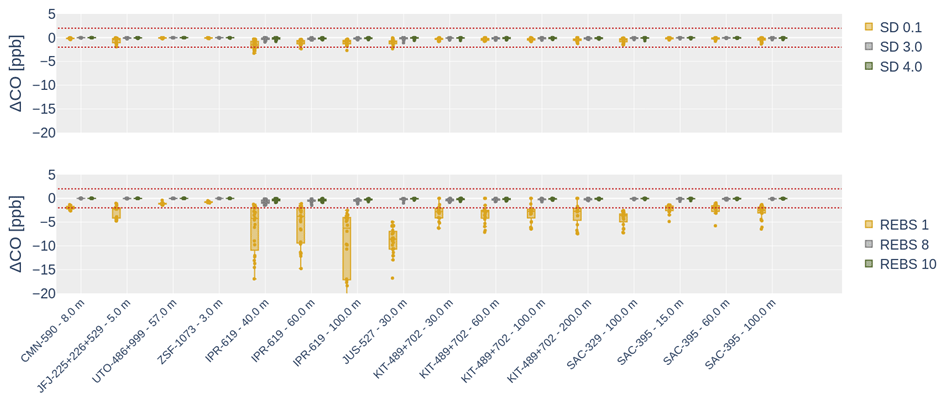
Figure 7 The same as Fig. 5 but for CO. The horizontal red lines represent the ±2 ppb WMO network compatibility goal.

To summarize, the remote sites (CMN, JFJ, ZSF, UTO) were less impacted by the de-spiking and the deviations of the de-spiked datasets in respect to the original ones were mostly within the WMO network compatibility goals. For the continental sites, larger deviations in respect to the original dataset were generally found after de-spiking with REBS, while significant deviations were observed for SD only for a limited number of sites and sampling heights.

3.4 Impact of the spike detections on diurnal cycles

We investigated how much the de-spiking methods influenced the seasonally averaged diurnal cycles of CO₂, CH₄ and CO at the test sites. To this aim, for each available time series, we calculated the average diurnal cycles for the original as well as for the de-spiked dataset using the different settings reported in Sect. 2.3 (for tall towers only the highest sampling heights were considered) for the individual seasons. Seasons were defined as December 2019–February 2020 (DJF), March–May (MAM), June–August (JJA) and September–November (SON). In this section, we only reported the results obtained for sites with significant impacts of the application of SD or REBS on the considered species; Figs. S1–S3 in the Supplement showed the analyses for all the methods, sites and species.

When looking at the results of de-spiking for CO₂ (Fig. S1), this analysis revealed that the application of SD had no impact on the shape of the 24 h mean cycles: the diurnal peaks detected for the original dataset were maintained for the de-spiked datasets. Only for the remote site ZSF was an impact observed during winter (Fig. 8). This was attributed to the wrong identification as a spike of a large CO₂ increase related to a regional-scale event, which was observed also at the near-mountain site of CMN (but without identification of spikes). For CO₂, a larger impact was found for REBS. In particular, when β=3 was adopted the diurnal peaks were smoothed at specific sites: JFJ and IPR (Fig. 8) and KIT and PUI (Fig. S1). Moreover, in some cases (see KIT, Fig. 8) the overall mean diurnal cycle was also modified.

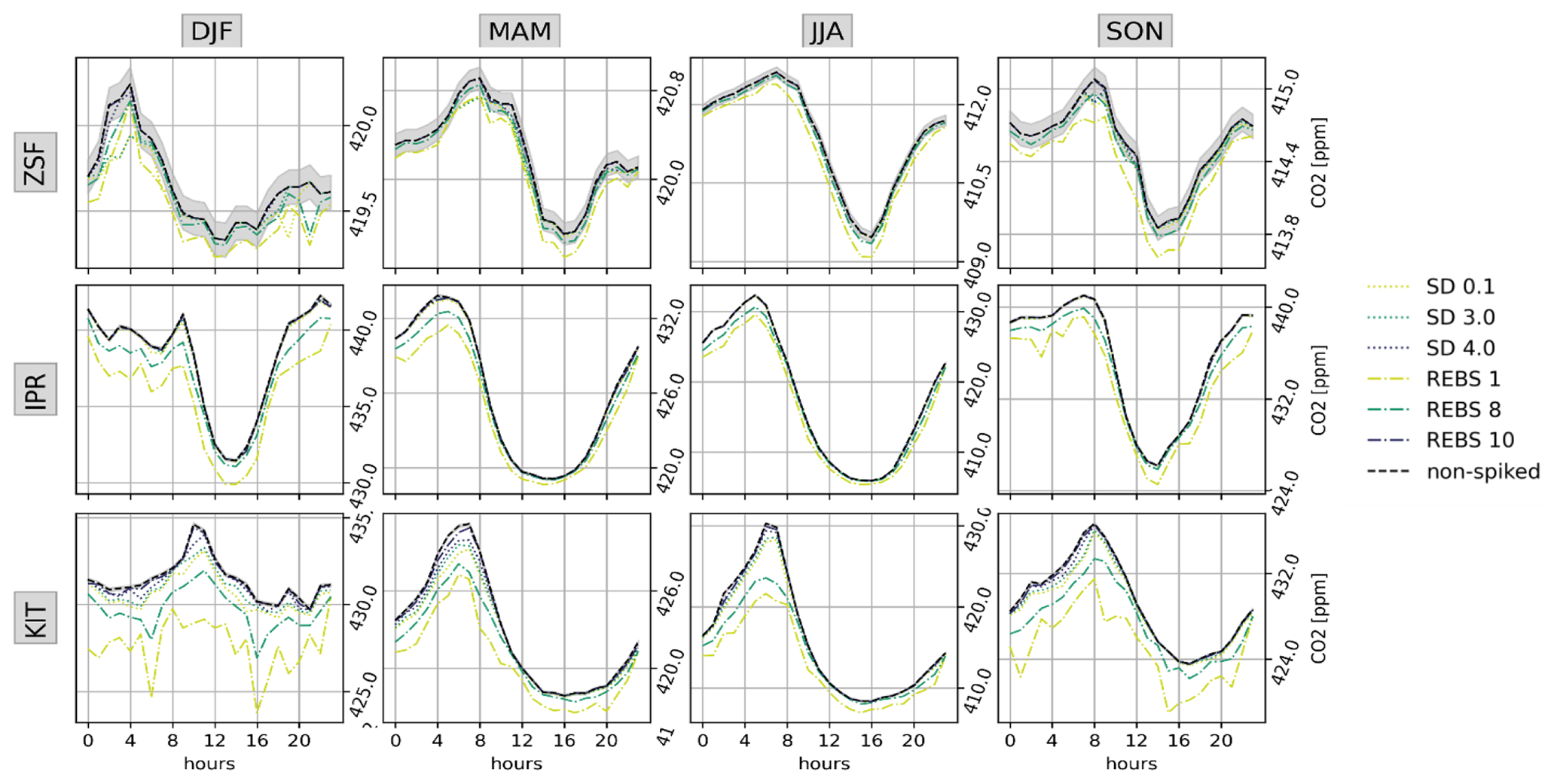
Figure 8 Mean seasonal diurnal cycles of CO₂ for different data selections and sampling heights at ZSF, IPR and KIT: results for the original data are shown (“non-spiked”) together with those after de-spiking for SD with $\mathit{\alpha }=\mathit{\{}\mathrm{0.1},\mathrm{1},\mathrm{4}\mathit{\}}$ and REBS with $\mathit{\beta }=\mathit{\{}\mathrm{1},\mathrm{3},\mathrm{10}\mathit{\}}$. The grey areas indicate the WMO network compatibility goal referring to the original dataset.

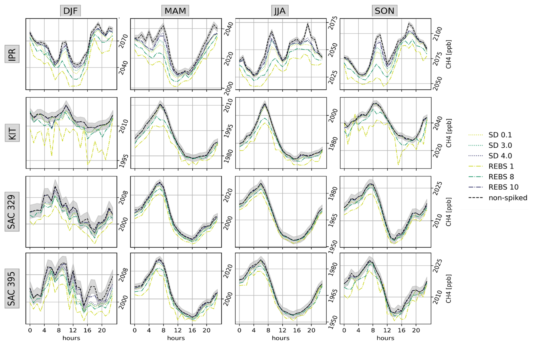
For CH₄, the application of the SD algorithm (α=1) led to a smoothing of the original diurnal peaks at IPR, KIT and SAC (Fig. 9), while no impacts were evident at the remote sites (Fig. S2). REBS (β=3) smoothed the original diurnal peaks at IPR and led to a decrease in the average values over the 24 h. According to the site PI, the diurnal peaks observed around 08:00 and 20:00 UTC at IPR, which were significantly smoothed by REBS, were related to very local sources of CH₄ due to the systematic venting of cattle farms located in the proximity of the site. As shown in Fig. 9, significant impacts by REBS were also evident at KIT and SAC for CH₄. Nevertheless, after the application of REBS (β=3), the winter diurnal cycle at KIT appeared more “noisy” in respect to the original dataset, suggesting the possibility of spike over-detection (13 % of data were identified as spikes for KIT at 200 m a.g.l.).

For CO (Fig. S3), significant deviations in respect to the original dataset were only observed when REBS with β=1 was considered.

Figure 9 The same as for Fig. 8 but for CH₄ at IPR, KIT, SAC 329 and SAC 395.

3.5 Comparison of SD and REBS spike detections during case studies

In this section, we analyze the ability of the SD and REBS methods in detecting spike events during specific case studies selected by the site PIs at JFJ, UTO, IPR, PUI, SAC and JUS. For each of the considered sites, a list of specific periods (lasting from a few days to a few weeks) affected by the occurrence of spikes were provided by the site PIs for CO₂, CH₄ and CO. SD and REBS were run for the standard configurations as well as for additional values of α (from 0.1 to 4.0) and β (from 1 to 10). Then, the spike identifications were inspected and evaluated by the site PIs, who also provided explanations for the possible origin of spikes. For each considered site and case study, a short description of the spike identification results was provided, together with expert assessment about the performance of the two methods. When possible, we also provided an evaluation about which method was in better agreement with the subjective judgment of the stations PIs for these specific case studies. For this objective, we varied the standard configurations (α and β values) and provided the optimal method configuration based on the subjective PI inspection of the de-spiking method results for each case study. Here, we provide a representative summary of the results by reporting a subset of the analyzed case studies, while the rest of them are presented in the Supplement (Figs. S4–S7 and Tables S1–S6).

Based on the case study analyses, both SD and REBS tended to overestimate spike occurrences with standard settings (see Sect. 3.1 for the definition of standard settings for SD and REBS) at JFJ (Table S1). As an example, here we report the case study for 19–21 November 2020 (Fig. 10). In this case, SD appeared to perform better than REBS overall. For CO₂, several data points of high variability were detected as spikes by SD in the afternoon of 21 November 2020, with a “false” detection on 19 November 2020 when a CO₂ increase due to the vertical transport of planetary boundary layer (PBL) air masses affected the measurement site. REBS was able to detect all the “high-variability” data points on 21 November but provided a larger number of false detections on the previous days (please note that the adoption of β=8, here not shown, would reduce the spike overestimation). For CH₄, SD was correct in not detecting spikes, while REBS over-detected spikes.

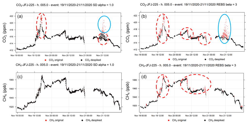
Figure 10 CO₂ and CH₄ observations at JFJ (19–21 November 2020). No-spike data are reported by the black points (“despiked”); red points (“original”) denote the data flagged as spikes using SD (a, c) and REBS (b, d). Circles with solid (dashed) outlines represent the spike attribution manually confirmed (not confirmed) by the site PI.

Moving to continental sites, by inspecting case studies at IPR, SD appeared to detect fewer spikes than REBS with standard settings for CO₂ and CH₄; by looking at CO, REBS also appeared to provide under-detection of spikes. As an example, we report the time series of trace gases at IPR from 2 to 4 July 2019 (Fig. 11). Systematic diurnal variability was evident for CO₂ with maxima in the morning and minima during afternoon–evening. Several spikes are superimposed onto this diurnal variability, but they were only marginally detected by SD. For CH₄, most of the spike events were identified by SD but only partially; i.e., SD underestimated the lower part of the events. For CO, basically no spikes were detected by SD, while REBS was able to catch only two major events (events occurring on 3 July were missed). On the other hand, it must be noted that REBS identified as spikes many data points not strictly related to spikes but lying on the “flanks” of large peaks. A test performed on IPR case studies suggested that decreasing β to 3 would increase the effectiveness of REBS in detecting CO spikes for the considered events.

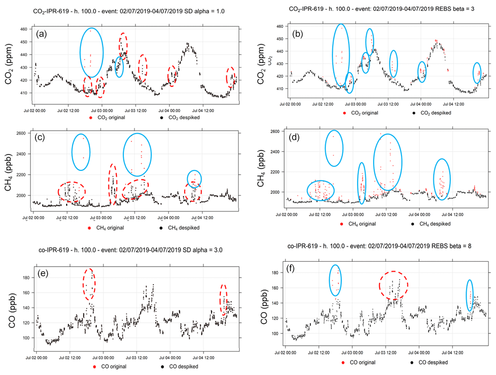
Figure 11 CO₂, CH₄ and CO observations at IPR (2 July 2019). No-spike data are reported by the black points (“despiked”); red points (“original”) denote the data flagged as spikes using SD (a, c, e) and REBS (b, d, f). Circles with solid (dashed) outlines represent the spike attribution manually confirmed (not confirmed) by the site PI.

The situation appeared to be different for the other continental site SAC. As deduced by the inspection of case studies, SD appeared to have more skills in detecting spikes than REBS when the standard configuration was used. An evident spike event for CO₂ and CH₄ occurred at SAC on 9–10 January 2019 (Fig. 12). The event was diagnosed by SD (for CO₂ the foot of the event was not detected) and by REBS. However, REBS provided an over-detection of spikes during the considered period: many data points embedded in CO₂ and CH₄ peaks were wrongly identified as spikes. As with the JFJ case study, increasing β to 8 (here not shown) would reduce the spike overestimation for REBS.

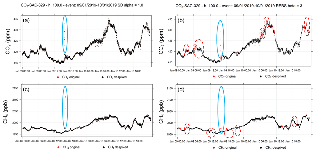
Figure 12 CO₂ and CH₄ observations at SAC (9–10 January 2019). No-spike data are reported by the black points (“despiked”); red points (“original”) denote the data flagged as spikes using SD (a, c) and REBS (b, d). Circles with solid (dashed) outlines represent the spike attribution manually confirmed (not confirmed) by the site PI.

3.6 Comparison between automatic and manual spike detections

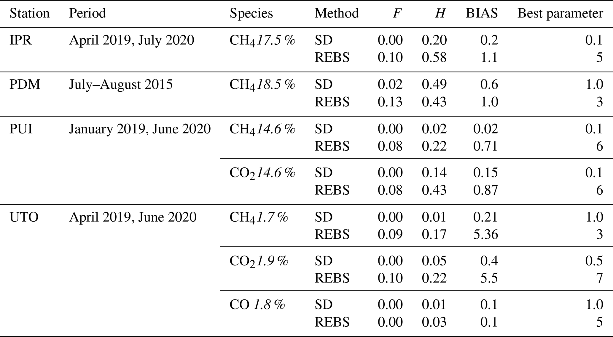
In this section, for a subset of sites (IPR, PUI, UTO), we present a comparison between the de-spiking operated by the methods and that made by the PIs of the sites. The test was carried out for a few months of observations (see Table 2). To have a sufficient number of spikes available for comparison, the subset of sites was selected to have at least 1 % of spike occurrences with respect to the whole dataset. In this context, the site PIs proceeded in manually flagging the data by adopting the same criteria and methodologies as those used during the routine data quality control. The results from this manual flagging were compared with the automatic flagging made by SD and by REBS. In this exercise, we also considered the CH₄ 1 min data recorded in July–August 2018 at Pic du Midi (PDM) that were analyzed by El-Yazidi (2018). Moreover, a wider range of the parameters α and β for SD and REBS was considered for this case study. In particular we used $\mathit{\alpha }=\mathit{\{}\mathrm{0.1},\mathrm{0.5},\mathrm{1.0},\mathrm{1.5},\mathrm{2.0},\mathrm{2.5},\mathrm{3.0},\mathrm{3.5},\mathrm{4.0}\mathit{\}}$ and $\mathit{\beta }=\mathit{\{}\mathrm{1},\mathrm{2},\mathrm{3},\mathrm{4},\mathrm{5},\mathrm{6},\mathrm{7},\mathrm{8},\mathrm{9},\mathrm{10}\mathit{\}}$. The methods were run for each of these parameters at IPR, PUI and UTO.

Table 2 False alarm rate (“F”), hit rate (“H”) and bias (“BIAS”) from the comparison of automatic (standard settings) and manual spike identifications. The optimal values for α (“SD”) and β (“REBS”) leading to the maximum agreement with the manual flagging are also reported (“Best parameter”). The periods over which the test was carried out are reported in the second column (“Period”) for each site, while the percentages of spikes identified by the site PIs are reported in the third column (italics).

The reported analysis was based on the calculation of metrics, for SD and REBS separately, that are used in order to evaluate the effectiveness of dichotomous weather forecasts (Thornes and Stephenson, 2001). Dichotomous forecasts are defined as forecasts that have two possible outcomes at most (e.g., forecasting the occurrence of fog at a given time and location). As well as for the case of weather forecasts, the SD and REBS methods provided a dichotomous identification of the spikes' occurrence by flagging each 1 min data point as “spike” or “no-spike”. After the automatic and the manual spike flagging, four possible outcomes were possible for each 1 min data point:

A

This denotes data flagged a spike by the automatic method and by the PI.

B

This denotes data flagged as spike by the automatic method but not flagged as spike by the PI.

C

This denotes data not flagged as spike by the automatic methods but flagged as spike by the PI.

D

This denotes data flagged as spike neither by the automatic methods nor by the PI.

Starting from these four possible outcomes, the following metrics were calculated for SD and REBS.

The hit rate H was calculated as follows:

$$\begin{array}{}\text{(3)}& H=p\left(f\mathrm{|}o\right)=A/(A+C),\end{array}$$

where p(f|o) is the conditional probability of automatically flagging a spike under the condition of having manually flagged a spike.

The false alarm rate F was calculated as follows:

$$\begin{array}{}\text{(4)}& F=p\left(f\mathrm{|}\underset{\mathrm{¯}}{o}\right)=B/(B+D),\end{array}$$

where $p\left(f\mathrm{|}\underset{\mathrm{¯}}{o}\right)$ is the conditional probability of automatically flagging a spike under the condition of not having manually flagged a spike.

The bias (BIAS) was calculated as follows:

$$\begin{array}{}\text{(5)}& \mathrm{BIAS}=(A+B)/(A+C),\end{array}$$

which is the ratio between the total number of forecasted spikes and the total number of observed spikes and should be as close as possible to 1.

Being based on the calculation of representative metrics and because the results of automatic spike detections were not shared with the site PIs, this exercise allows a more objective evaluation of the spike detection methods and also provides information that could be used to potentially identify the “optimal” de-spiking configuration at each site.

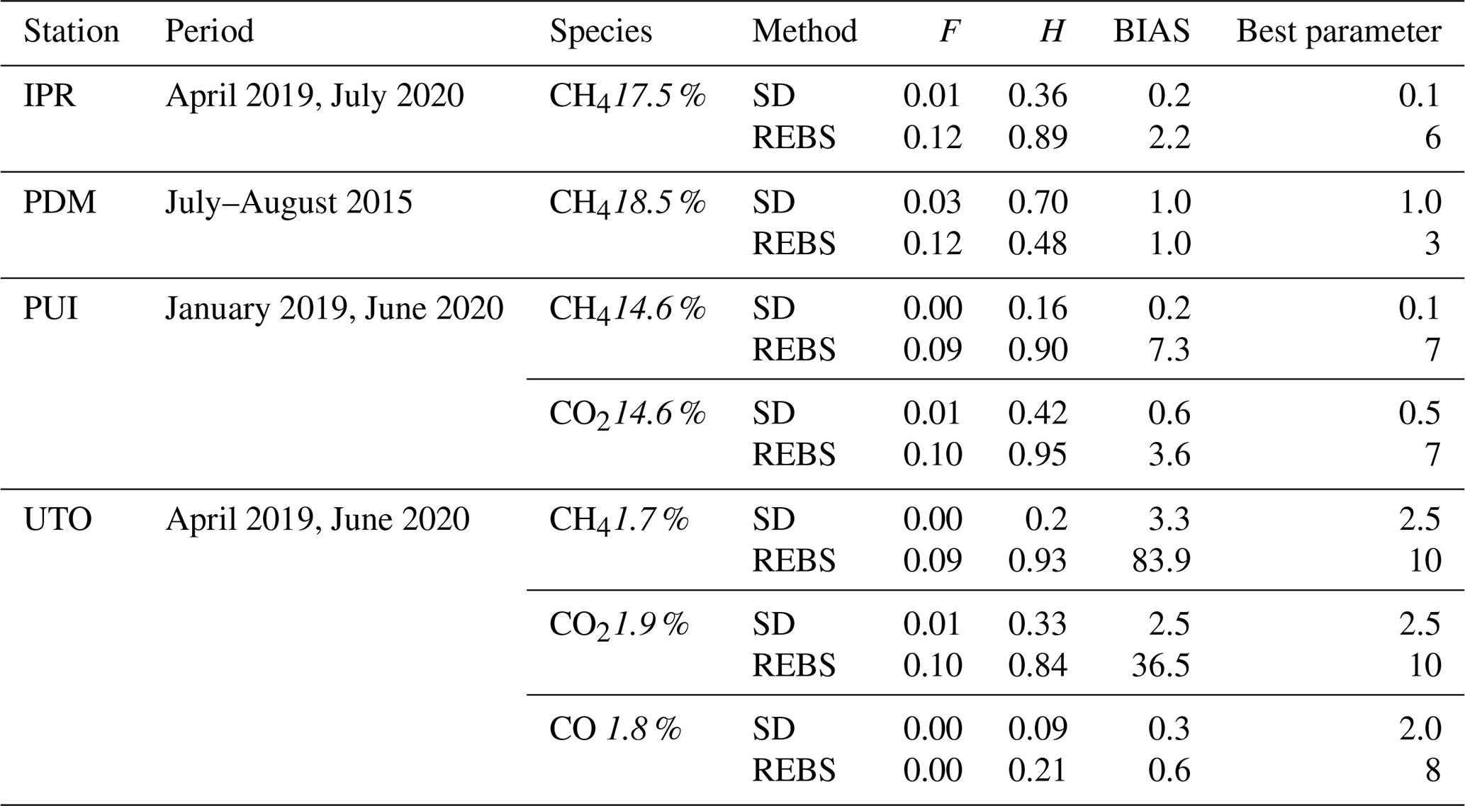
Table 3 The same as Table 2 but with results from the high-spike analysis.

In this comparison exercise, we considered the spikes manually detected by PIs to be the “real” (or reference) spikes. This choice is related to the fact that PIs were familiar with the site characteristics and were constantly involved in the analysis and validation of the raw data; thus they represented the most authoritative experts to assess the occurrence of spikes at their own sites. However, it can be argued that the manual selection performed by the site PIs could also be affected by some degree of “inaccuracy” and cannot be considered a perfect reference. As an example, the manual flagging can be less accurate when very frequent spikes affect the time series, making the manual selection of spikes very demanding. Moreover, the manual flagging, like any human data screening, could be affected by a certain degree of arbitrariness. Thus the results of this comparison should not be strictly interpreted as an assessment of the quality of the automatic algorithm performance.

The results of this analysis are reported in Table 2 for the application of the methods to the 1 min data of CO₂, CH₄ and CO. In general, it was difficult to find a case for which an optimal agreement existed between the automatic and the manual spike selection. Compared to SD, REBS detected more spikes which were also identified by the site PIs (see the larger H values) but also more events which were not recognized as spikes by the PI manual flagging (see the larger F values). Only for PDM (CH₄) did the application of SD lead to higher H values. By excluding the PDM case for CH₄, REBS had better BIAS than SD.

A further analysis was then conducted on “high” spikes in order to evaluate the agreement between automatic and manual de-spiking on a subset of spikes that were expected to have a strong impact on the average values of the time series. In order to perform this analysis, high spikes were defined as the 1 min data points whose distance from a 1 h rolling-mean baseline was higher than 0.5 ppm for CO₂ and 2 ppb for CH₄ and CO. A sensitivity study was performed by changing the value of the spike selection thresholds, but no evident deviations were found compared to using 0.5 ppm and 2 ppb.

Compared with the all-spike analysis, both SD and REBS were more effective in catching high-spike events (see the higher values for H in Table 3). Especially for REBS, high H values were obtained, indicating that REBS detected a large fraction of the high spikes manually identified by PIs. However, BIAS strongly increased in respect to the analysis that also included lower-amplitude spikes (especially for REBS), indicating a strong tendency in overestimating the number of events in respect to the PI selection.

By inspecting the variations in H, F and BIAS as a function of α and β, we tried to identify an optimal algorithm setup for each site and chemical species (i.e., the best agreement among manual and automatic detection), and we report them in Tables 2 and 3. For CO₂ and CH₄, under the all-data selection, for four out of seven cases, the best agreement between the two methods was achieved when the α parameter was lowered to 0.1–0.5 for SD and the β parameter was increased to values of 5–7 for REBS. For REBS, this implied a decrease in F to values comparable with SD and a decrease in H to lower values (thus implying lower effectiveness of REBS in detecting spikes) but an increase in the degree of consistency of the results provided by the two methods.

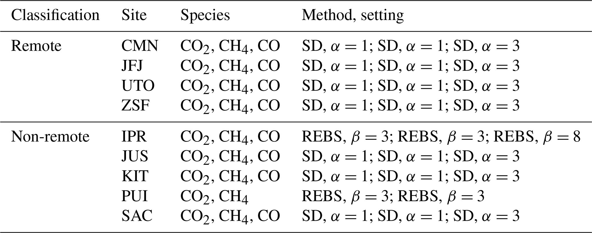
Table 4 List of specific method and setting currently adopted for each considered site. Sites are listed in alphabetical order according to their classifications (remote, non-remote).

4 Discussion and conclusions

In this exercise, we considered a subset of different atmospheric sites (i.e., remote, continental, urban) for which SD and REBS spike detection methods were applied to 1 min data of CO₂, CH₄ and CO. Sensitivity studies were performed in order to compare the impact of the two methods to the original datasets in terms of spike frequency and hourly and monthly mean values as well as seasonal diurnal cycles. Case studies were considered to test the ability of the automatic methods in identifying spikes. Finally, “blind” tests were executed to objectively compare with a dichotomous analysis the agreement between the spikes manually identified by the site PIs and by the automatic methods.

One main outcome of this study was that REBS identified a larger number of spikes than SD and was less “site-sensitive” than SD for CO₂ and CH₄. On average, considering all time series, REBS detected about 10 times more spikes than SD. This led to a larger impact of REBS on the monthly averaged values and on the seasonally averaged diurnal cycle of CO₂ and CH₄: in respect to the original dataset, the application of REBS (with β={1, 3}) led to significant impacts (i.e., deviations larger than the WMO network compatibility goal) for all the non-remote sites. On the other hand, SD reported impacts only for selected continental sites. For CO, significant deviations in respect to the original dataset were observed only for REBS with β=1. As shown by the analysis of the 1 h datasets, both SD and REBS were able to narrow the original data distribution or shift it towards lower values.

The application of the automatic methods to the case studies showed that it was challenging to identify one common algorithm and/or configuration for all the considered sites. Significant differences in the ability of detecting spikes were observed as a function of the sites, events and considered species. The analyses of selected case studies (reported in the Supplement) would suggest that REBS performed better than SD at specific sites (i.e., IPR and PUI).

The comparison of SD and REBS with the blind manual flagging made by the site PIs at four sites (IPR, PDM, PUI and UTO) showed that both the automatic methods were able to select only a portion of the spike events identified by the site PIs (i.e., hit rate lower than 58 %). REBS was better than SD in successfully detecting the spikes selected by the manual identification (hit rate ranged from 0.17 to 0.58 for REBS and from 0.01 to 0.33 for SD) but with the cost of selecting a very large fraction of data not recognized as spikes by the site PI (false alarm rate ranged from 0.08 to 0.12 for REBS). However, this did not necessarily imply less accuracy for REBS: especially in the case of frequent spike occurrence, it cannot be completely ruled out that spike events could be missed by the PI manual identification. When high spikes were considered, the hit rate increased for both REBS (ranging from 0.21 to 1.00 as a function of the site) and SD (ranging from 0.02 to 0.75) but with REBS strongly overestimating the number of spikes (BIAS > 1) in respect to the manual identification. In particular, it should be noted that in the case of a low frequency of spike occurrence, REBS appeared to strongly over-detect the spike occurrence (BIAS higher than 10). Interestingly, based on this comparison, it was pointed out that decreasing the α parameter to 0.1–0.5 for SD and increasing the β parameter to 5–7 for REBS led to more consistent spike identification results between the two methods.

For REBS a further test was carried out by increasing the temporal window over which the baseline $\widehat{g}\left(t_i\right)$ was calculated to 10 and 30 d. The test was carried out using β=3 for eight sites (CMN, JFJ, UTO, IPR, KIT, PUI, SAC, JUS). The considered case studies revealed that increasing the time window led to a strong overestimation in the number of spikes. As descriptive examples, the Supplement reports two case studies for SAC. Moreover, REBS (with β=3) was also run on the time series of the 1 min CH₄ standard deviation values (instead of on the 1 min mean values). The aim of this test was to assess the ability of REBS in detecting records characterized by high variability at timescales lower than 1 min (see Supplement). In respect to the standard application to the 1 min mean values, the adoption of this configuration significantly increased the number of the detected spikes by 50 %–70 % (as a function of the site), implying a large number of false spike detections. On the other hand, some obvious spike events were partially missed for a few sites (CMN, JFJ, PUI, SAC), thus suggesting that running REBS on the time series of 1 min standard deviations was not a suitable strategy to automatically detect spikes.

To summarize, for the considered measurement sites, neither SD nor REBS appeared to provide a perfect identification of the spike events, but SD is less prone to spike over-detection that could introduce inconsistencies in the data record. It was shown that the REBS tendency to over-detect the spike occurrence could lead to significant biases in the calculation of the monthly and seasonal mean values in respect to the original data record. This would suggest extreme caution should be exercised in adopting REBS as an operational method to perform automatic spike detection at the atmospheric ICOS stations. Based on the experiment results, we recommend that REBS is implemented only for specific sites, mostly affected by more or less frequent very nearby local emissions (like IPR and PUI), where clear benefits in using REBS were demonstrated. Table 4 summarizes the combination of method/setting which has been operationally implemented at the analyzed test sites by taking into consideration the results of this experiment and the need to standardize as much as possible the detection method among the sites. The strategy for the implementation of these automatic spike detection methods is to flag the 1 min data without removing them from the data collection: this gives the data users the opportunity to decide whether to consider the original dataset or the de-spiked dataset depending on their specific data usage purposes.

Our results were only in partial agreement with the outcomes of El Yazidi et al. (2018), who applied SD and REBS to a CH₄ record which was occasionally subject to very local pollution: this former study reported that REBS had a notable tendency to not catch a certain fraction of the spikes, while SD correctly detected most of the contaminated data. This suggested that the effectiveness of the automatic spike detection by SD and REBS could be site-specific. Thus, it is recommended to perform sensitivity experiments to evaluate and document the performance of the implemented detection method, including its setting. Even if the adoption of common documented standardized methods to detect the occurrence of spikes further increases the already-high traceability and the transparency of the ICOS data production chain, further activities are needed for better consolidating the fitness for purpose of the two proposed methods as well as their specific settings as a function of the different sites. More information could be obtained by the operational implementation of the automatic de-spiking methods over the whole ICOS network. This information can be used to adopt future refinements in the method settings devoted to the optimization of the automatic de-spiking. These refinements can include the possibility of modifying the current settings of SD and REBS (i.e., α and β values); of combining the CO₂, CH₄ and CO spike detection; of including other diagnostic parameters (e.g., wind speed and direction, bottom-up emission data); and of tuning and/or selecting the methodology as a function of the different sites by adopting approaches like that proposed in Sect. 3.6. Moreover, a specific strategy should be developed for the few stations within the ICOS network using buffer volumes (i.e., Svartberget, Norunda, Hyltemossa, Hyytiälä and Cabauw). One possibility is to implement deconvolution (see Winderlich et al., 2010), followed by the application of the spike detection. A further action to be pursued is the exchange of experiences with other initiatives or measurement networks in the atmospheric composition landscape (e.g., the Aerosol, Clouds and Trace Gases Research Infrastructure – ACTRIS RI – or the Advanced Global Atmospheric Gases Experiment – AGAGE) with the aim of considering different or novel (e.g., machine-learning-based) spike detection methods or combing the information that comes from different chemical species (e.g., synthetic compounds or NO_x) to improve the attribution of detected spikes.