W-band S–Z relationships for rimed snow particles: observational evidence from combined airborne and ground-based observations

Values of undercatch-corrected liquid-equivalent snowfall rate (S) at a ground site and microwave reflectivity (Z) retrieved using an airborne W-band radar were acquired during overflights. The temperature at the ground site was between −6 and −15 ^∘C. At flight level, within clouds containing ice and supercooled liquid water, the temperature was approximately 7 ^∘C colder. Additionally, airborne measurements of snow particle imagery were acquired. The images demonstrate that most of the snow particles were rimed, at least at flight level. A relatively small set of S–Z pairs (four) is available from the overflights. Important distinctions between these measurements and those of Pokharel and Vali (2011), who reported S–Z pairs and an S–Z relationship for rimed snow particles, are (1) the fewer S–Z pairs, (2) the method used to acquire S, and (3) the altitude, relative to ground, of the W-band Z retrievals. This analysis corroborates the fact that the S–Z relationship reported in Pokharel and Vali (2011) yields an S – in scenarios with snowfall produced by riming – substantially larger than that derived using an S–Z relationship developed for unrimed snow particles.

1 Introduction

Improvement of methods used to measure snowfall and rainfall is an ongoing focus of meteorological research. The various methods use ground-based instruments that evaluate the mass of precipitation that falls into or onto a collector (precipitation gauges) (Brock and Richardson, 2001), ground-based radars (Wilson and Brandes, 1979), and airborne and spaceborne radars (Matrosov, 2007; Kulie and Bennartz, 2009; Geerts et al., 2010; Skofronick-Jackson et al., 2017). An objective of these approaches, whether used to make observations independent of other methods (e.g., Kulie and Bennartz, 2009) or as a component of multiple observations (e.g., Cocks et al., 2016), is the estimation of precipitation rate and accumulated precipitation amount

Many studies have investigated using radar to evaluate rainfall (for a review see Wilson and Brandes, 1979). There are two approaches. The first is research, both observational and computational, that probes the relationship between rainfall rate (R) and radar-measured values of range-corrected backscattered microwave power. The latter is commonly reported as an equivalent radar reflectivity factor (Z_e). The second is operational in the sense that precipitation gauges are used to calibrate measurements acquired using weather surveillance radars. Complications associated with converting Z_e to R, or converting a radar reflectivity factor¹ (Z) to R, can be grouped in four categories: (1) inaccuracy in quantification of Z, (2) variation of the R–Z relationship stemming from precipitation processes (e.g., coalescence and break-up), (3) differences between the volume of a radar range gate versus the much smaller volume of atmosphere sampled as precipitation falls to a gauge, and (4) vertical displacement between a radar range gate and a calibrating gauge, especially at far ranges.

For situations with snowfall, methods employing either a gauge or radar are associated with complications beyond those incurred in rainfall (Matrosov, 2007; Martinaitis et al., 2015; Cocks et al., 2016). Problems associated with gauge measurements are wind-induced snow particle undercatch, gauge capping, delayed registration, and blowing snow aliasing as snowfall. Moreover, in a situation with snow particles more abundant within a radar range gate compared to raindrops and where a measurement of Z is used to infer R via an R–Z relationship, the resultant precipitation rate will likely be inaccurate. This is because hydrometeor shape, density, and dielectric properties are all variable for snow particles, while they are relatively invariant for raindrops. Additionally, a snow particle's terminal fall speed varies with size (as is the case for drops) as well as with particle shape and particle density. Going forward, we refer to the latter two properties as shape and density.

The goals of this paper are as follows: (1) to describe measurements of undercatch-corrected liquid-equivalent snowfall rate (S, mm h⁻¹) and how these were paired with W-band measurements of reflectivity (Z, mm⁶ m⁻³), (2) to contrast the S–Z pairs against S–Z relationships commonly applied in radar retrievals of S, and (3) to investigate why the S–Z pairs deviate from predictions of some S–Z relationships.

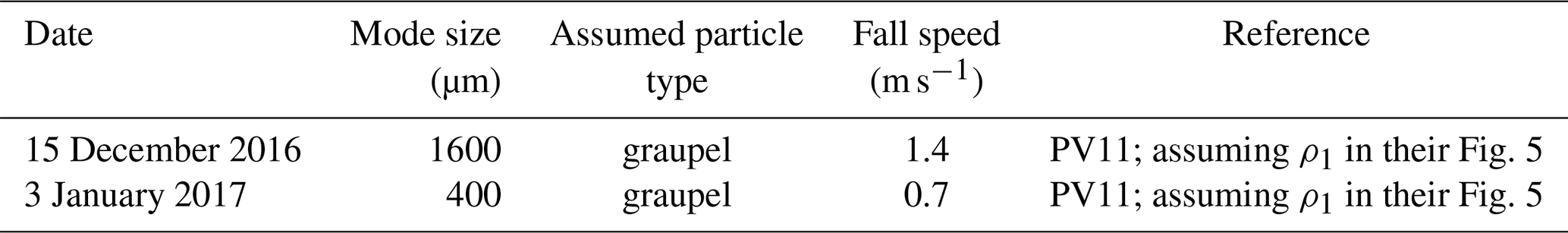
In calculations of paired values of S and Z, density is an important parameter. Density is commonly estimated using empirical data (e.g., Pokharel and Vali, 2011; PV11). For graupel, a snow particle that grows via collection of supercooled cloud droplets in a process commonly referred to as riming, paired observations of particle mass and particle size have been used to estimate density. There is considerable uncertainty in this approach. Based on data collected at two northwestern US surface sites (Zikmunda and Vali, 1972; Locatelli and Hobbs, 1974), density values differ by at least a factor of 2 at particle sizes smaller than 2000 µm (PV11; their Fig. 4). Given that the density of rime ice varies with droplet impact speed, droplet size, and temperature (Macklin, 1962), it is not surprising that the density–size relationships analyzed by PV11 are so varied.

Table 1 and the following paragraphs overview W-band S–Z relationships applied in instances with snow particles grown by vapor deposition (crystal), by collection of crystals (aggregate snowflake), and by riming (rimed crystal and graupel). Henceforth, the latter two snow particle types are collectively referred to as rimed snow particles.

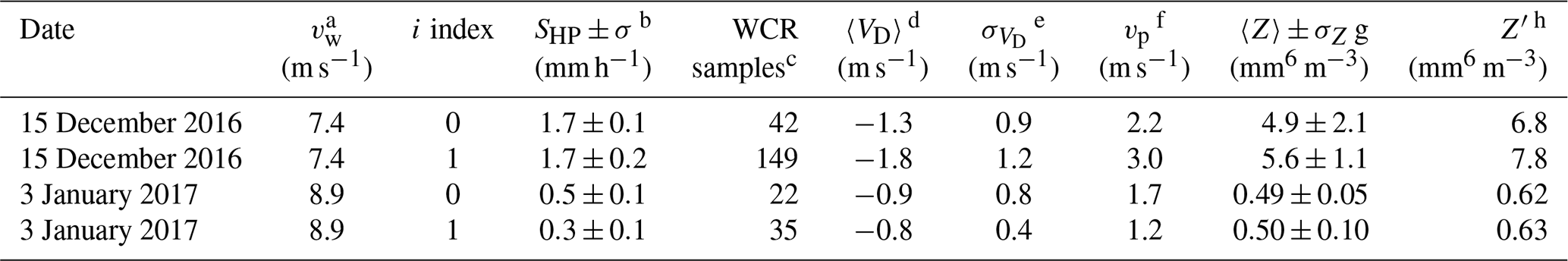
Table 1 W-band S–Z relationships from the literature, snow particle type, and values of minimum relative S difference.

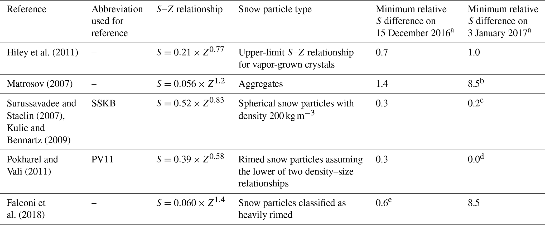
^a Minimum relative S difference is defined as the minimum of $\mathrm{|}(S_{\text{HP}}-S)\mathrm{|}/S$ where S_HP is a measurement of undercatch-corrected liquid-equivalent snowfall rate (Table 6) and S is a snowfall rate on an S–Z relationship line evaluated at one of the attenuation-corrected reflectivities (Sect. 4). ^b Attenuation-corrected Z on this day (0.6 mm⁶ m⁻³) is smaller than the lower-limit Z (1 mm⁶ m⁻³) advised for this S–Z relationship (Matrosov, 2007). ^c Maximum relative S difference on this day is 0.4. ^d Maximum relative S difference on this day is 0.7. ^e Maximum relative S difference on this day is 0.9.

In a computational study, Hiley et al. (2011) considered a variety of snow particle types (column, plate, bullet rosette, sector plate, dendrite, and aggregate snowflake), employed a parameterized ice particle size distribution (PSD) function (Field et al., 2005), accounted for a range of temperature (−5 to −15 ^∘C) via the Field et al. parameterization, and developed a range of S–Z relationships for snow particles. Except for the aggregate snowflakes (henceforth, aggregates), the modeled particle types were vapor-grown crystals. The Hiley et al. upper- and lower-limit relationships are S = 0.21 × Z^0.77 and S = 0.024 × Z^0.91, respectively. Matrosov (2007) developed an S–Z relationship for aggregates. In that work, parameterized PSDs from Braham (1990) were employed, and a range of particle aspect ratios were factored into the calculations. For aggregates, the S–Z relationship is S = 0.056 × Z^1.2 (Matrosov, 2007). It should be noted that Hiley et al. (2011) and Matrosov (2007) employed similar, but not identical, computational methods. Computational research was also conducted by Kulie and Bennartz (2009), who adopted the wavelength-dependent density derived by Surussavadee and Staelin (2007) (200 kg m⁻³ at λ = 3.2 mm), modeled the snow particles as spheres, and applied PSDs based on Field et al. The resultant S–Z is S = 0.52 × Z^0.83 (Surussavadee and Staelin, 2007; Kulie and Bennartz, 2009; henceforth, SSKB). Variance in the calculations discussed in this paragraph originates from changes in density, shape, fall speed, PSD, and particle size as these changes are propagated through the cloud microphysical and microwave-scattering calculations.

In a hybrid approach (computational and an analysis of measurements), PV11 concluded that most of the snow particles they imaged were rimed snow particles. Values of S were calculated using a density–size function (ρ₁, discussed below), a fall speed–size function, measured PSDs and measured particle images, and a determination of particle volumes. It was assumed that a prolate spheroid approximated particle shape and that shape was the basis for determining a particle's sphere-equivalent volume and the particle's sphere-equivalent size. The sphere-equivalent size was applied in the two functions. Values of Z were calculated using a measured PSD, sphere-equivalent sizes, the ρ₁ function, and Mie theory. PV11 presented calculations of Z, obtained using two density–size relationships (their Eqs. 1 and 2), and compared their calculated reflectivities to measurements of Z from a W-band radar. That led to their conclusion that “…the lower density assumption… yielded closer correspondence to observed reflectivities.” Their recommendation for S as a function of measured Z – hereafter the $S\left({\mathit{\rho }}_{\mathrm{1}}\right)/Z$ best-fit line – is S = 0.39 × Z^0.58. Values of Z that were paired with the calculated values of S (i.e., the S–Z pairs from PV11 that we present in Sect. 4) and that were used to determine the $S\left({\mathit{\rho }}_{\mathrm{1}}\right)/Z$ best-fit line came from the W-band radar. In addition to variance in their values of S, coming from a dependence on density, PV11 state that a value of S derived via their best-fit line is uncertain by a factor of 10. That uncertainty is evident in the variance of S–Z data pairs about the $S\left({\mathit{\rho }}_{\mathrm{1}}\right)/Z$ line in Fig. 11 of PV11. Those investigators, and Geerts et al. (2010), attributed the variance to use of two-dimensional snow particle images in calculations of S and to actual variations of density, shape, and particle size not accounted for in the calculations.

Another set of hybrid-type S–Z relationships was developed by Falconi et al. (2018; their Table 2). These are based on measurements from a video disdrometer, weighing precipitation gauge, microwave radiometer, and vertically pointing W-band radar. All these systems were operated at the ground. The data set was stratified into intervals of lightly rimed, moderately rimed, and heavily rimed snow. A proxy for snow particle riming – radiometer measurements of liquid water path – was the basis for the stratifications (von Lerber et al., 2017). The S–Z relationships are S = 0.10 × Z^1.0 (lightly rimed), S = 0.079 × Z^1.3 (moderately rimed), and S = 0.060 × Z^1.4 (heavily rimed).

Our focus is on surface measurements of S and on pairing of those measurements with airborne measurements of Z. We also analyze airborne measurements of snow particle imagery. The latter demonstrate that the particles observed at flight level were rimed. The imagery is the basis for our assertion that our data set is relevant to ongoing investigations of using Z to evaluate S in situations in which precipitation is produced by riming.

Section 2 describes the setting of our study, the instruments we deployed, and recordings we obtained using two data acquisition systems. One of the data systems was operated at a ground site and the other on an aircraft. Section 3 is an analysis of the recordings; this section also considers recordings from two additional, but ancillary, ground sites. Our findings are discussed in Sect. 4 and summarized in Sect. 5. Appendix A explains how we averaged recordings of near-surface W-band reflectivities and surface-based recordings of snowfall.

2 Site, aircraft, and instruments

2.1 Site

Analyzed herein are aircraft and ground data from 14–15 December 2016 and from 3 January 2017. The ground data were acquired in a forest–prairie ecotone on the eastern slope of the Medicine Bow Mountains in southeastern Wyoming (Fig. 1a and b). No ground-based observers were deployed during the two snowfall events analyzed.

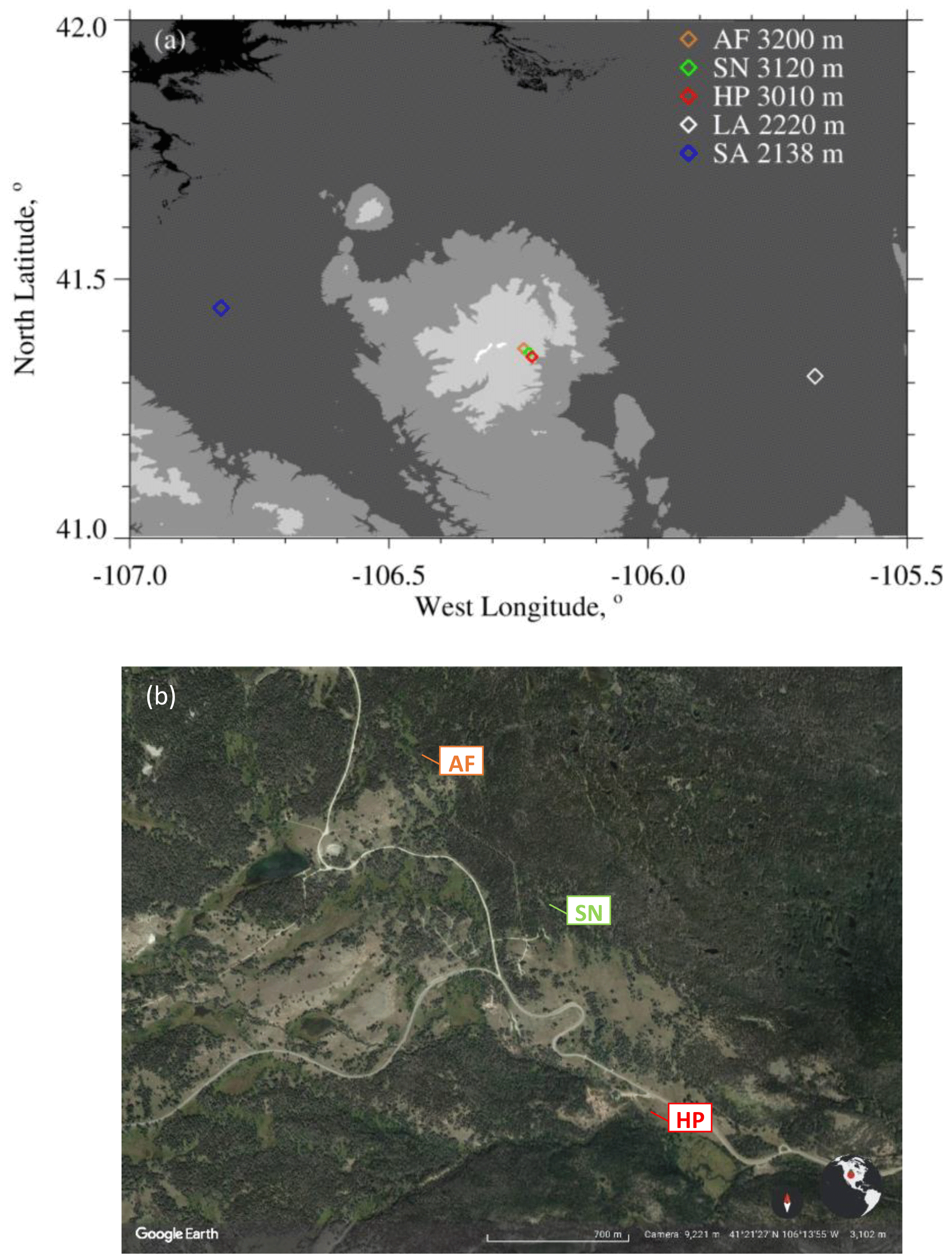
Figure 1 (a) Southeastern Wyoming: airport at Saratoga (SA), airport at Laramie (LA), and the ground sites. AF: US-GLE AmeriFlux tower, SN: Brooklyn Lake SNOTEL, and HP: hotplate. Altitudes of the airports and ground sites are in the legend. Altitude thresholds for the digital elevation map are 1500, 2000, 2500, 3000, and 3500 m. (b) Close-up of the AF, SN, and HP ground sites (from © Google Earth).

At one of three ground sites (HP in Fig. 1a and b) a hotplate precipitation gauge (Rasmussen et al., 2011; Zelasko et al., 2018), a GPS receiver, and a data acquisition system were deployed. Once per second, the data system ingested a hotplate-generated data string, combined that with time of day from the GPS receiver (Coordinated Universal Time, UTC), and recorded the merged hotplate–UTC data string. The absolute accuracy of the time stamp is no worse than 2 s.

Overflights of the hotplate were done by the University of Wyoming King Air (WKA) on 14–15 December 2016 and on 3 January 2017. The flights were conducted in preparation for the SNOWIE field project (Tessendorf et al., 2019) and were flown from the Laramie, WY, airport (LA in Fig. 1a). Data acquisition on the WKA was also synchronized with UTC, but with much better accuracy than at the hotplate.

Measurements of horizontal wind (speed and direction), temperature, relative humidity, and pressure from the US-GLE AmeriFlux tower (AF in Fig. 1a and b) are also components the analysis. The AmeriFlux data were provided to us as 30 min averages (AmeriFlux, 2023; Marlow et al., 2023).

2.2 University of Wyoming King Air (WKA)

The following WKA measurements were analyzed: aircraft position, temperature, snow particle imagery, and three moments of the cloud droplet size distribution function. A cloud droplet probe (CDP; Faber et al., 2018) was the basis for the droplet size distribution measurements and the derived moments. The latter are droplet concentration (N), cloud liquid water content (LWC), and mean droplet diameter (〈D〉). Snow particle imagery was obtained using a precipitation particle imaging probe (2DP; Korolev et al., 2011) and a cloud particle imaging probe (2DS; Lawson et al., 2006). These acquired two-dimensional images of particles between 200 and 6400 µm (2DP) and between 10 and 1280 µm (2DS).

2.3 The W-band Wyoming Cloud Radar (WCR)

Retrievals from the up-looking and down-looking antennas of the WCR, operated on the WKA, were also analyzed. For this we used Level 2 WCR data² with reflectivities recorded as dBZ = 10 × log₁₀(Z). The reflectivities were converted from dBZ to Z prior to processing. Additionally, values of the vertical-component Doppler velocity retrieved from below the WKA using the WCR's down-looking antenna were analyzed. The Doppler velocities were corrected for aircraft motion as described in Haimov and Rodi (2013). We use V_D to symbolize the corrected vertical-component Doppler velocity and adopt the convention that V_D > 0 indicates upward hydrometeor motion.

The Level 2 WCR sampling was different on the 2 flight days and this difference is shown in Table 2. Ground-based calibrations of the WCR's up-looking antenna and correlations between in-flight retrievals acquired using the WCR's up-looking and down-looking antennas were used to estimate the precision and absolute accuracy of the WCR-derived values of dBZ. These are ± 1.0 and ± 2.5 dBZ, respectively (PV11).

Table 2 Level 2 WCR sampling and the WKA overflight time.

2.4 Hotplate gauge

Algorithms used to process hotplate measurements are described in Rasmussen et al. (2011), Boudala et al. (2014), and Zelasko et al. (2018). Henceforth, these are referred to as R11, B14, and Z18, respectively. This section describes how hotplate measurements acquired at the HP site were analyzed. The hotplate deployed at the HP site is described in Wolfe and Snider (2012), Z18, and Marlow et al. (2023).

Five measurements fundamental to the steady-state energy budget of the hotplate's temperature-controlled up-viewing plate are output by the hotplate microprocessor as 1 min running averages (Z18). These averages were merged with the GPS time and recorded at 1 Hz by the data acquisition system (Sect. 2.1). With these measurements, calibration data (Marlow et al., 2023), and the algorithm developed by Z18, we calculated S in two steps. First, the five hotplate measurements (electrical power supplied to the plate, ambient temperature, wind speed, downwelling shortwave flux, and downwelling longwave flux) were input to Eq. (3) in Z18. The output of that equation is a provisional liquid-equivalent precipitation rate. Second, the snow particle catch efficiency, described in the next paragraph, was used to calculate S as the ratio of the provisional rate and the catch efficiency.

Marlow et al. (2023; their Fig. 3b) report the relationship between snow particle catch efficiency and wind speed that was applied in the calculation of S. There are three bases for this relationship. First is the catch efficiencies R11 derived using measurements obtained from a weighing gauge, operated within a double-fence intercomparison reference shield, and collocated measurements from an unshielded hotplate gauge. These paired measurements are denoted as SRG (shielded reference gauge) and UHG (unshielded hotplate gauge). R11 plotted hotplate catch efficiencies (i.e., UHG $/$ SRG) versus wind speeds measured at 10 $\mathrm{m}\mathrm{a}.\mathrm{g}.\mathrm{l}.$ (their Fig. 8). Second is the Marlow et al. (2023) adjustment of R11's 10 $\mathrm{m}\mathrm{a}.\mathrm{g}.\mathrm{l}.$ wind speeds to 2 m a.g.l. The basis for the adjustment is surface boundary layer parameters derived for R11's site (Kochendorfer et al., 2018) and an equation from Panofsky and Dutton (1984; their Eq. 6.7). The adjustment was made because the hotplate-derived wind speeds, both here and in Marlow et al. (2023), were acquired at approximately 2 m above the snowpack surface. Third is the Marlow et al. (2023) comparison of SNOTEL-derived liquid-equivalent depth changes and hotplate-derived time-integrated accumulations. The interval for the comparisons is 24 h. Based on the comparison, which has 57 paired values acquired at the sites labeled HP and SN in Fig. 1, the average fractional absolute relative difference is 0.30. Marlow et al. (2023) also provided an estimate of the error in a SNOTEL measurement (2.4 mm). At an accumulation of 10 mm the error corresponds to a relative error of 0.24. This indicates that SNOTEL contributed significantly to the SNOTEL–hotplate variance, especially so for the smaller accumulations in Fig. 9a of Marlow et al. (2023). Because of this, we do not limit the following estimate of hotplate precision to a subset of the 57 paired measurements. Based on our assessment of the average fractional absolute relative difference, the hotplate precision applied in this analysis was taken to be 0.3.

The hotplate-derived wind speeds acquired at ∼ 2 m and discussed in the previous paragraph are henceforth symbolized by U_PRO. The basis for these is a steady-state energy budget of the hotplate's temperature-controlled down-viewing plate and a proprietary algorithm (R11 and Z18). The U_PRO values are reported by a hotplate as 1 min running averages (Z18) and we recorded these at 1 Hz. Examples are the gray dots in Fig. 2. Additionally, we calculated 1 min averaged values of U_PRO and the corresponding standard deviations. Examples of these are the black circles and the short vertical line segments in Fig. 2.

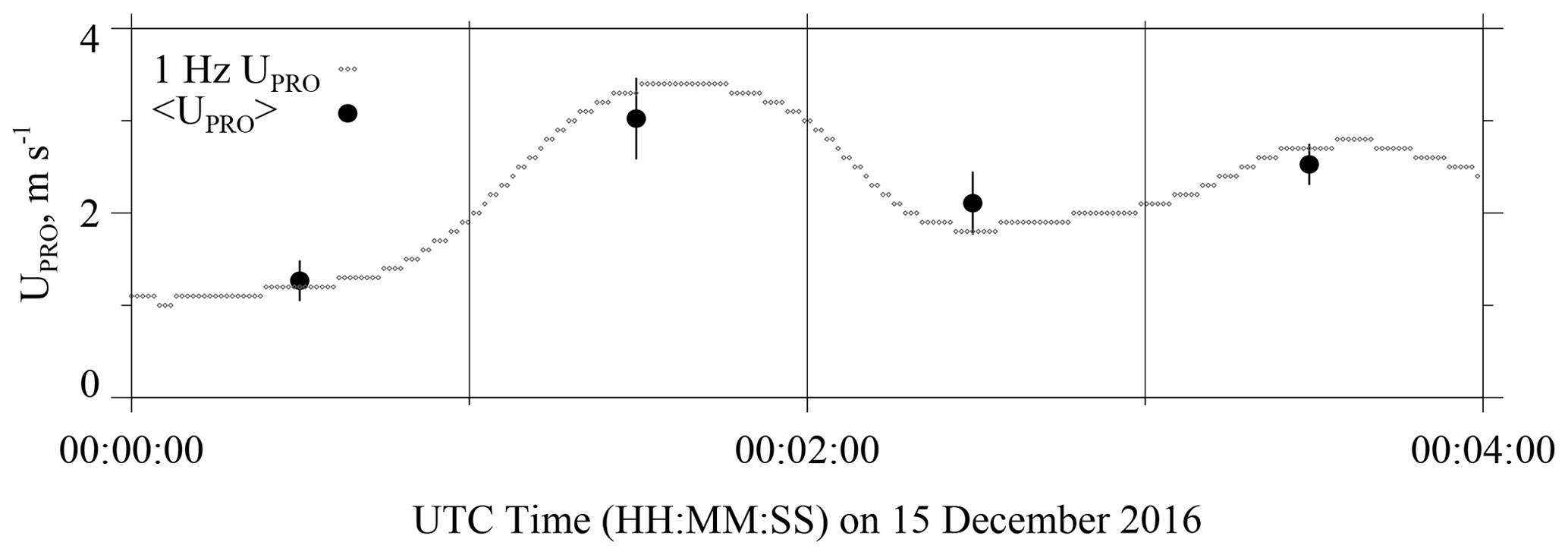
Figure 2 Hotplate wind speed measurements (U_PRO) from 00:00:00 to 00:04:00 UTC on 15 December 2016. Gray dots are the 1 min running-average U_PRO recorded at 1 Hz. Black circles are the 1 min averaged U_PRO (± 1 standard deviation).

3 Analysis

3.1 WKA overflight time

The focus of our analysis is the two WKA flight segments shown in Fig. 3a and b. The maps shown in the figure have the three ground sites (AF, SN, and HP) and the WKA flight tracks (white line). The beginning to end time interval for the flight tracks is 100 s, and these are divided into 10 intervals of 10 s each. The 10 s intervals are indicated with white diamonds. Except for the turn evident in Fig. 3b, the flight tracks are straight, and the track direction is approximately upwind to downwind.

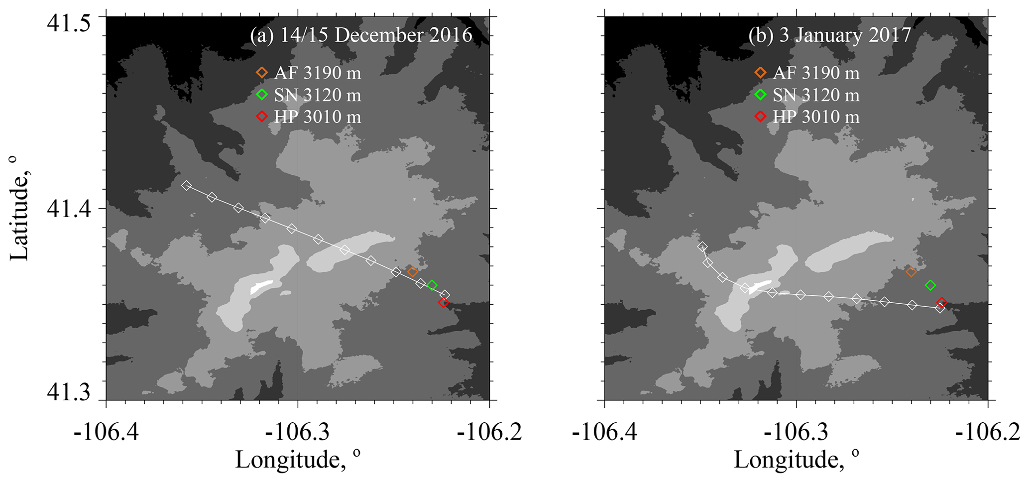
Figure 3 (a) WKA flight track on 14–15 December 2016 for a time interval calculated as the overflight time − 100 s to the overflight time. (b) WKA flight track on 3 January 2017 for a time interval calculated as the overflight time − 100 s to the overflight time. The white diamonds on the tracks are separated in time by 10 s. Altitude thresholds for the digital elevation maps are 2600, 2800, 3000, 3200, 3400, and 3600 m. Altitudes of the ground sites are in the legend.

Times when the WKA was closest to the HP site were evaluated by finding the point on the flight track where the horizontal position of the WKA was closest to the hotplate's coordinates. These times are symbolized by t₀ and are referred to as overflight times. In Fig. 3a and b the downwind end of the flight tracks end at the overflight time. The latitude–longitude position of the aircraft was within 390 m of the hotplate at the overflight times. Table 2 has the overflight times on the 2 flight days.

3.2 Effect of attenuation on WCR reflectivities

The presence of molecular oxygen, water vapor, cloud water, and snow particles within the WCR's transmission path will contribute to an attenuation of microwave intensity and will therefore negatively bias the retrieved reflectivities (Matrosov, 2007; Hiley et al., 2011; Kneifel et al., 2015). Models of attenuation, radar remote sensing, and in situ measurements were used to calculate this bias. For oxygen, an attenuation coefficient from Ulaby et al. (1981; their Fig. 5.6) as well as temperature (T) and pressure (P) measurements from the AF (Table 3) were used. For vapor, an attenuation coefficient (Ulaby et al., 1981; their Eq. 5.22) as well as T, P, and relative humidity (RH) measurements from the AF (Table 3) were used. Concentrations of oxygen and water vapor and the oxygen and vapor path lengths are provided in Table 4. The latter is the vertical distance between the HP and the WKA. It was assumed that concentrations were uniform over this path length.

Table 3 Atmospheric state averages.

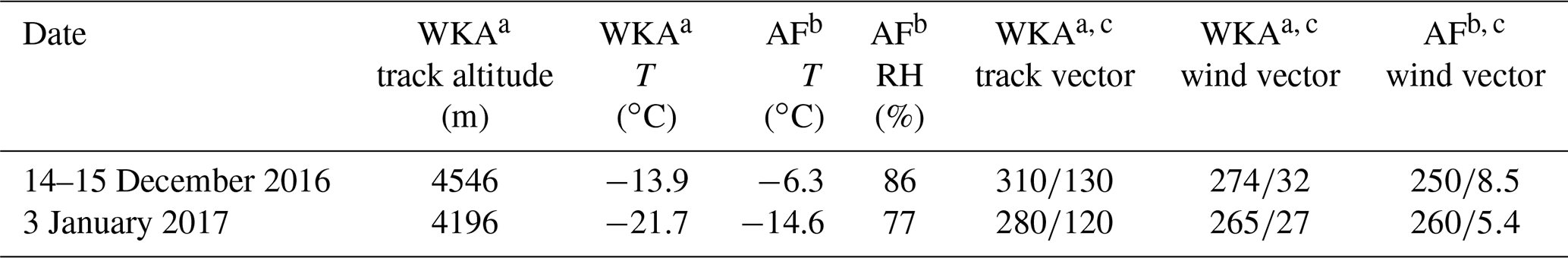
^a Altitude, temperature, track vector, and horizontal wind vector data obtained by averaging 1 Hz WKA measurements. The averaging interval is 60 s, and the interval starts at the overflight time minus 60 s and ends at the overflight time. ^b Temperature (T), relative humidity (RH), and horizontal wind vector data from sensors on the US-GLE AmeriFlux tower (Sect. 2.1). The wind sensor was deployed at 26 $\mathrm{m}\mathrm{a}.\mathrm{g}.\mathrm{l}.$ (3223 $\mathrm{m}\mathrm{m}.\mathrm{s}.\mathrm{l}.$), and the T and RH sensor was deployed at 23 $\mathrm{m}\mathrm{a}.\mathrm{g}.\mathrm{l}.$ (3220 $\mathrm{m}\mathrm{m}.\mathrm{s}.\mathrm{l}.$). The AF measurements correspond to 30 min averages closest to the overflight time. In the AF data set, time stamps on the relevant AF recordings are 00:00 UTC (15 December 2016) and 20:30 UTC (3 January 2017). ^c Vectors are presented in the following format: direction of motion (degree relative to true north)$/$speed (m s⁻¹).

Attenuation by cloud water was derived using the WKA-measured T (Table 3), the WKA-measured LWC, path length (Table 4), and an attenuation formula (Liebe et al., 1989; Vali and Haimov, 2001). The LWC applied in the formula is the maximum of CDP measurements acquired between t₀ − 10 s and t₀. This interval coincides with the interval in which the WCR's down-looking antenna was used to acquire reflectivities over the HP (Sect. 3.5). The path length for cloud water was derived as the vertical distance between cloud base (derived thermodynamically using AF measurements; Table 3) and flight level. LWC was assumed to be uniform at the maximum value over the path length.

Table 4 Attenuating component concentration, one-way pathlength, and the overall two-way attenuation.

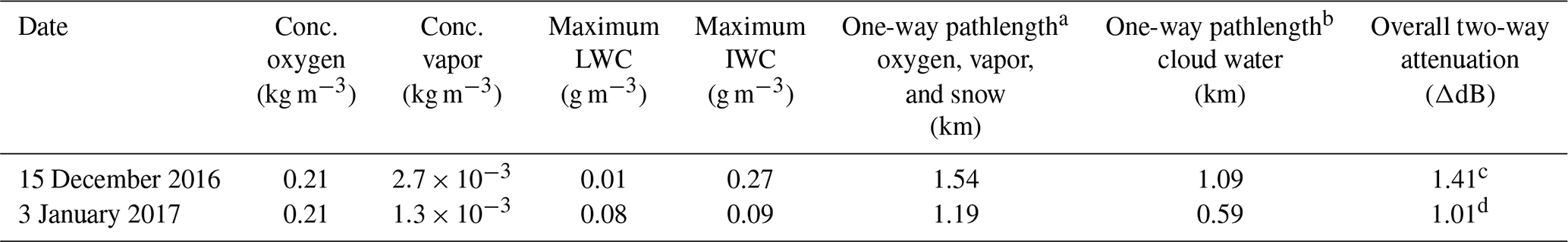
^a Vertical distance between HP and WKA. ^b Vertical distance between cloud base (derived thermodynamically using AF measurements; Table 3) and WKA. ^c One-way attenuation coefficients are 0.03 dB km⁻¹ for oxygen (Ulaby et al., 1981), 0.14 dB km⁻¹ for vapor (Ulaby et al., 1981), 0.056 dB km⁻¹ for cloud water (Liebe et al., 1989; Vali and Haimov, 2001), and 0.24 dB km⁻¹ for snow particles (Nemarich et al., 1988). ^d One-way attenuation coefficients are 0.03 dB km⁻¹ for oxygen (Ulaby et al., 1981), 0.073 dB km⁻¹ for vapor (Ulaby et al., 1981), 0.49 dB km⁻¹ for cloud water (Liebe et al., 1989; Vali and Haimov, 2001), and 0.077 dB km⁻¹ for snow particles (Nemarich et al., 1988).

Snow particle mass concentration is typically reported as an ice water content (IWC, g m⁻³) (Liu and Illingworth, 2000). The contribution of IWC to attenuation was calculated using measurements in Nemarich et al. (1988), who reported an attenuation coefficient equal to 0.9 dB km⁻¹ per unit of IWC. Also used were retrievals of IWC acquired using the down-pointing WCR antenna. There are several steps in the calculation. First, all profiles of dBZ acquired between t₀ − 10 s and t₀ were selected. Second, a maximum dBZ was selected at each of the down-beam range gates (Table 2). Third, the dBZ maxima were increased by the overall two-way attenuation in the final column of Table 4. Fourth, the profile of attenuation-corrected dBZ was converted to a profile of attenuation-corrected Z. Fifth, a Z-to-IWC parameterization was applied (IWC = 0.10 × Z^0.51; PV11; their Table 3). Sixth, the IWC profile was integrated, and the derived ice water path was divided by the snow particle path length (Table 4). This calculation produced a time- and range-averaged maximum IWC (Table 4). This IWC is the value applied in the attenuation calculation.

Two-way attenuations (ΔdB), summed over contributions from the four components, are presented in the final column of Table 4. Attenuation by snow and attenuation by liquid were the most important components (> 50 %) on 15 December and 3 January, respectively. Vapor contributed 32 % overall on 15 December, and the combination of vapor and snow contributed 45 % on 3 January. Equation (1) shows how an attenuation-corrected reflectivity (Z^′) was derived using an uncorrected reflectivity (Z) and the ΔdB.

$$\begin{array}{}\text{(1)}& Z^{\prime }={\mathrm{10}}^{\left[[\mathrm{10}\cdot {\text{log}}_{\mathrm{10}}(Z)+\mathrm{\Delta }\mathrm{dB}]/\mathrm{10}\right]}\end{array}$$

3.3 Correction of Doppler velocity

We accounted for bias in V_D (Sect. 2.3) due to deviation of the down-looking WCR antenna from vertical. This was done by applying the correction described in Zaremba et al. (2022) (their Eq. A4). The west-to-east and south-to-north particle velocities used in the correction were assumed to be equal to component wind velocities. The latter were expressed as linear functions of altitude using the information in the penultimate and last columns of Table 3. The component velocities as functions of altitude and the linear equations relating velocity and altitude are provided in Appendix A.

3.4 Hotplate measurement of wind speed

Here we compare the hotplate-derived wind speed to wind speed derived using an R.M.Young rotating anemometer (R.M.Young; model 05103). The second of these is symbolized by U_RMY, and the basis for the first (U_PRO) is a proprietary algorithm (Sect. 2.4). We are doing this comparison because B14 showed that U_PRO can be high-biased relative to a conventional anemometer and because U_PRO is the primary determinant of the rate at which the up-viewing plate dissipates sensible heat energy. Diagnosis of that heat transfer rate is our basis for calculating the liquid-equivalent snowfall rate (Z18). The U_PRO also determines the snow particle catch efficiency, and the latter was used in calculations of the undercatch-corrected liquid-equivalent snowfall rate (Sect. 2.4).

The comparisons reported here were done at the Laramie, WY, airport in December 2019 and in January 2020. Compared to the HP site, the Laramie airport site (indicated by LA in Fig. 1) is free of obstruction out to 120 m and experiences larger wind speeds. By mounting the hotplate and the R.M.Young anemometer on rigid metal pipes, the hotplate's heated horizontal surfaces (the up- and down-viewing plates seen in Fig. 1 of Z18) and the anemometer's spinning axis (oriented horizontally) were both positioned at 2 $\mathrm{m}\mathrm{a}.\mathrm{g}.\mathrm{l}.$ The pipes were separated horizontally by 5 m. There was no precipitation on the days selected for the wind speed comparisons. The values of U_PRO and U_RMY we analyzed were recorded with a data system that time-stamped the 1 Hz U_PRO and 1 Hz U_RMY with a relative timing accuracy no worse than 1 s.

A wind speed comparison – from 13 December 2019 – is shown in Fig. 4a. U_PRO was brought into the comparison by sampling it once per minute from files containing 1 Hz recordings of the 1 min running-average U_PRO (Sect. 2.4). U_RMY was brought into the comparison by starting with files containing 1 Hz recordings and converting these to 1 min averages. Figure 4a shows no evidence of bias and Fig. 4b demonstrates that the average absolute departure between the U_PRO and U_RMY (both 1 min averages) is no larger than 1 m s⁻¹. Table 5 has eight more precipitation-free comparisons. Included in the table are temperature and wind speed averaged over the comparison intervals (04:00 to 20:00 UTC), the slope of the linear-least-squares fit line (forced through the origin, red line), and the lower and upper quartiles of the slope. The quartiles were calculated using the method of Wolfe and Snider (2012). In contrast to Fig. 4a and b, Fig. 4c and d make the comparison using 1 Hz values of U_PRO and U_RMY. The larger scatter and larger average absolute departure seen in these panels are a consequence of the hotplate's limited time response compared to the R.M.Young. We quantify the hotplate's response time in terms of a calculated thermal response time. During wintertime at the Laramie airport and with wind speed at 5 m s⁻¹, the down-viewing plate's thermal response time is approximately 60 s (results not shown). Because the temperature of the down-viewing plate is actively controlled, this does not translate to a 60 s lag between changes in wind speed and the hotplate response. The U_PRO–U_RMY departure is most evident at U_PRO > 5 m s⁻¹ (Fig. 4d), but this is not a concern for U_PRO on 14–15 December 2016 or on 3 January 2017. Snider (2023b) demonstrated that the U_PRO was less than 5 m s⁻¹ at the hotplate during the two WKA overflights.

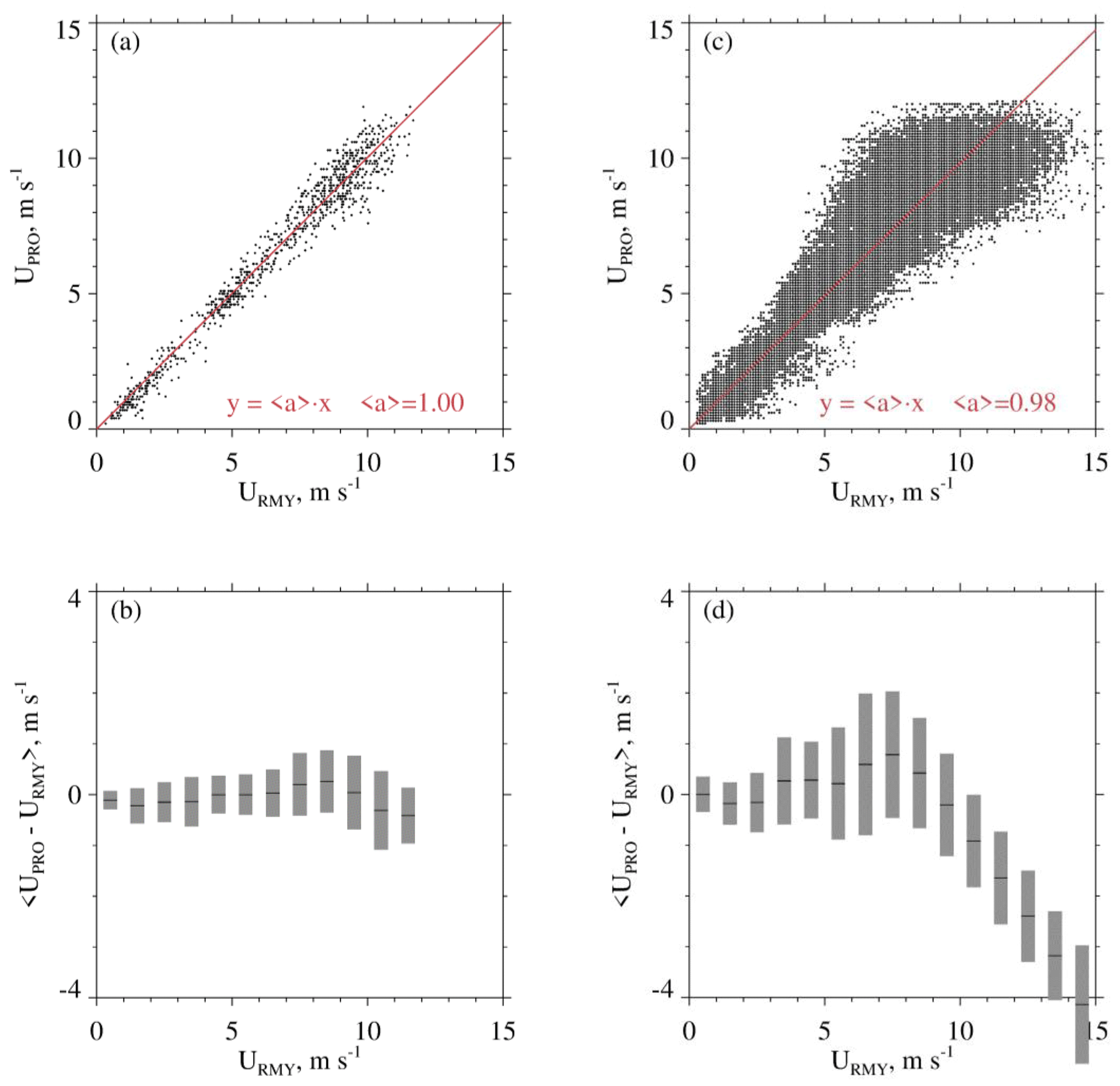
Figure 4 (a) Scatterplot of 1 min averaged U_PRO and 1 min averaged U_RMY. Measurements were acquired at the Laramie, WY, airport on 13 December 2019. The red line is a linear-least-squares fit line (forced through the origin). (b) Average departure between 1 min averaged U_PRO and 1 min averaged U_RMY. Average departures were calculated for discrete U_RMY intervals, and the averages are indicated with short black horizontal lines. Gray bars indicate ± 1 standard deviation. (c) Same as in panel (a) except for 1 Hz values of U_PRO and U_RMY. (d) Same as in panel (b) except for 1 Hz values of U_PRO and U_RMY.

Table 5 U_PRO versus U_RMY correlations.

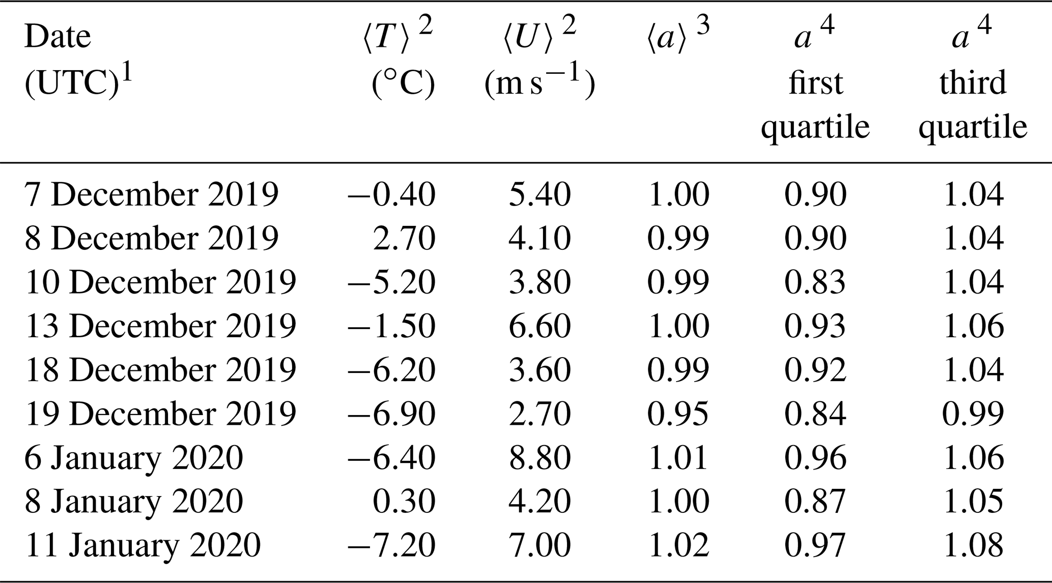
¹ Statistics presented are based on 1 min averaged U_PRO and 1 min averaged U_RMY measurements made between 04:00 and 20:00 UTC. ² Interval-averaged temperature and interval-averaged wind speed. ³ Slope of the 1 min averaged U_PRO versus 1 min averaged U_RMY linear-least-squares fit line, forced through the origin. ⁴ Quartiles of the slope (see text).

3.5 Combined aircraft and surface measurements

Figure 5 has WCR and WKA measurements starting 100 s prior to t₀ and ending at t₀. The sequences in Fig. 5a and c are reflectivities from both the up- and down-looking antennas. In Fig. 5a the flight track (dashed black horizontal line) is at 4550 m, and in Fig. 5c the flight track is at 4200 m. At the t₀ in Fig. 5a, below the WKA, the maximum radar echo is +6 dBZ (Z = 4 mm⁶ m⁻³), and in Fig. 5c the maximum is −3 dBZ (Z=0.5 mm⁶ m⁻³). Supercooled liquid water was detected as the aircraft approached the ridgeline (Fig. 5b) and during the last 10 s of the time sequence in Fig. 5d. During these encounters with supercooled liquid, the maximum LWC values were 0.03 × 10⁻³ and 0.08 × 10⁻³ kg m⁻³ on 14 December 2016 and 3 January 2017, respectively. Values of N (Sect. 2.2) at times of maximal LWC were 3 × 10⁶ and 100 × 10⁶ m⁻³ on 14 December 2016 and 3 January 2017, respectively. Even on 3 January 2017, the 〈D〉 (Sect. 2.2) associated with maximum LWC was sufficient for hexagonal plate crystals with diameters larger than 100 µm to collide with the observed droplets with efficiencies > 0.1 (Wang and Ji, 2000).

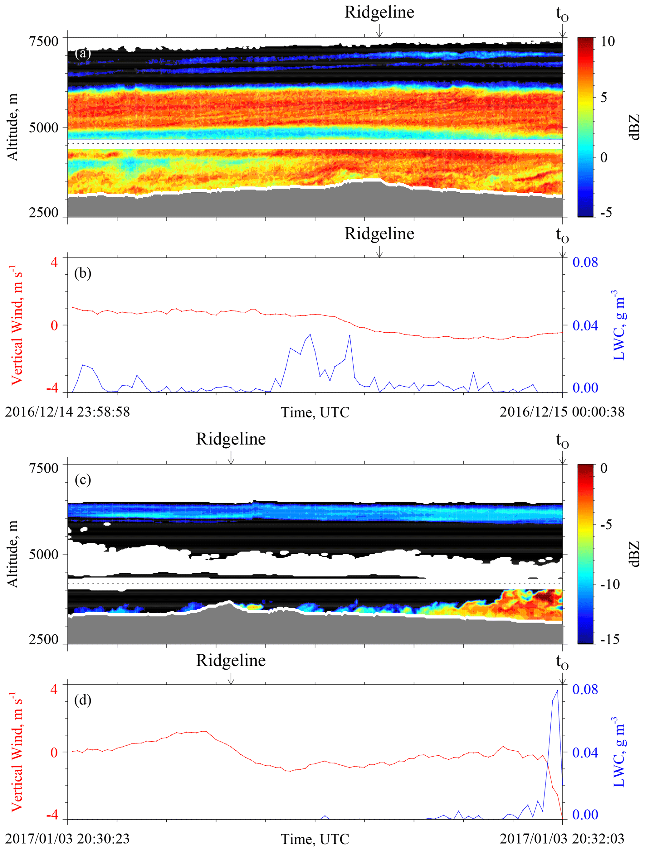
Figure 5 (a) 100 s of WCR reflectivity and (b) 100 s of LWC and gust probe vertical wind velocity ending at t₀ on 14–15 December 2016. (c) 100 s of WCR reflectivity and (d) 100 s of LWC and gust probe vertical wind velocity ending at t₀ on 3 January 2017. In panels (a) and (c), above and below the flight track, the roughly 200 m deep WCR blind zone is evident. Reflectivity above (below) the flight track is from the up-looking (down-looking) WCR antenna. Black indicates dBZ values smaller than the minimum indicated in the color bar, white immediately above the terrain indicates echo that was discarded because of ground clutter, and white above the ground clutter and outside the blind zone indicates dBZ less than the minimum detectable signal.

We temporally and spatially averaged the values of Z we compared with time-averaged values of S. There are two reasons for this: (1) as discussed in Sect. 3.1, the WCR did not sample Z exactly over the hotplate, and furthermore, the width of the radar beam at 1500 m range – roughly the distance between the aircraft and the ground at the overflight times – is 30 m and thus considerably smaller than the minimum horizontal distance between the aircraft and the HP. (2) Compared to the WCR, the hotplate is a relatively slow-response measurement system whose output is commonly averaged over 1 min intervals (Z18).

In our analysis, the HP measurements were averaged over two adjacent 60 s intervals. The first extends from t₀ to t₀ + 60 s (Fig. 6a) and the second from t₀ + 60 s to t₀ + 120 s (Fig. 6c). In Fig. 6a and c, t_HP,B symbolizes an interval's beginning time and t_HP,E symbolizes an interval's ending time. Formulas describing how these times were related to the beginning and ending time of a corresponding WCR averaging interval are in Appendix A. Figure 6b is a schematic of the first WCR averaging interval and Fig. 6d is a schematic of the second. Again, the subscripts “B” and “E” are used to indicate averaging beginning and ending times. Figure 6b and d have lines at the top of an averaging interval and/or domain. The slopes of these lines are proportional to the ratio of two speeds. These speeds are a maximum likely snow particle speed toward the ground (v_p) and a horizontal wind advection speed (v_w). The v_pwas calculated using averaged vertical-component Doppler velocities and v_w was calculated using a vertical profile of horizontal winds based on WKA horizontal wind measurements and AF horizontal wind measurements (Fig. A1a and b) and using the WKA track vector (Table 3). An altitude ($z^{\prime }=\mathrm{3400}$ m) was assumed in the calculation of v_w. This is the altitude of the ridges west and northwest of the HP site (Fig. 3a and b). Picking the altitude to be either $z^{\prime }=\mathrm{3200}$ m or $z^{\prime }=\mathrm{3600}$ m does not alter our findings.

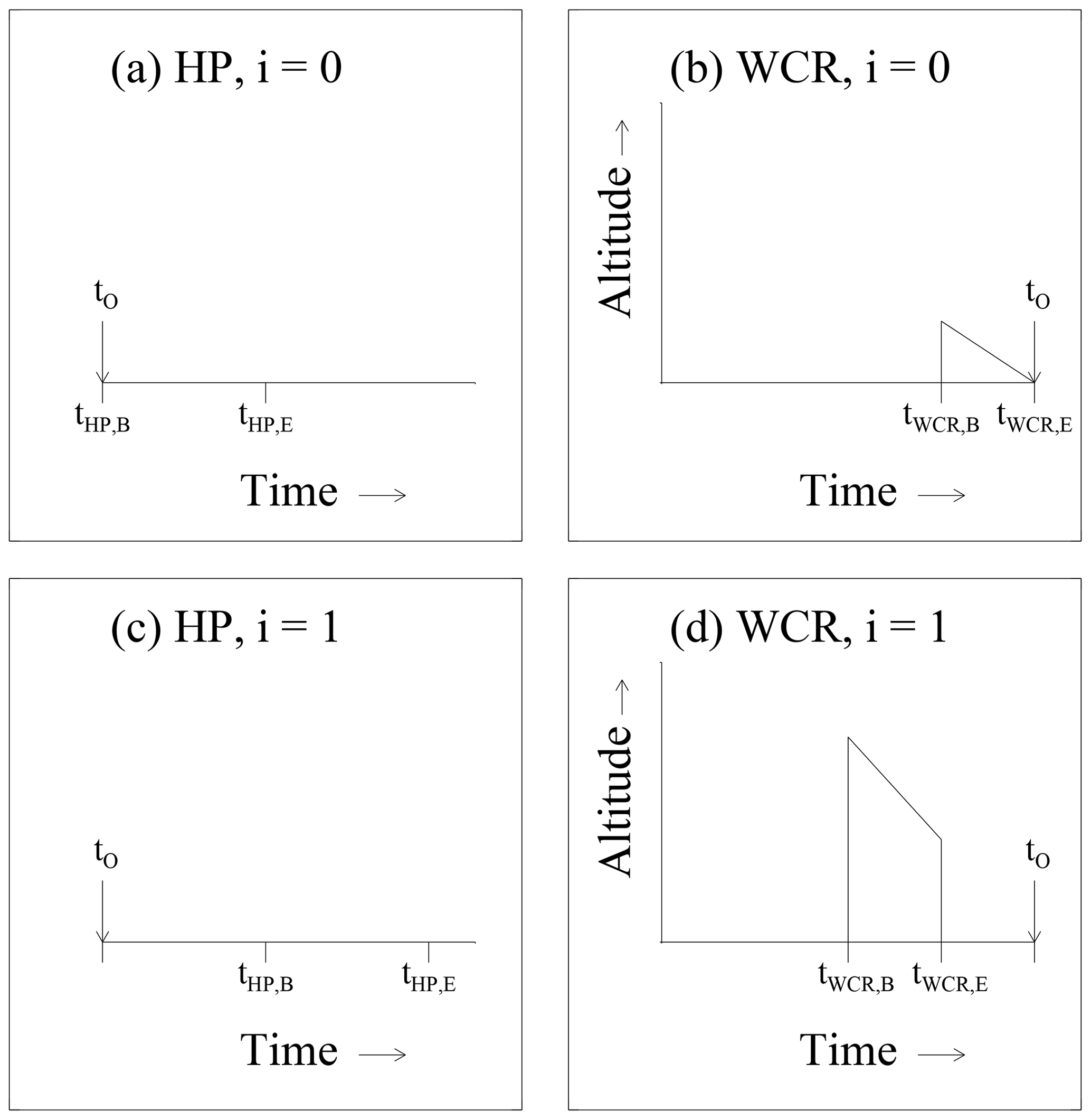
Figure 6 (a, c) Representations of the i=0 and i=1 HP averaging intervals. (b, d) Representations of the i=0 and i=1 WCR averaging domains. The t₀ is shown in all panels. The subscripts “B” and “E” indicate beginning and ending times of the HP averaging (a, c) and the beginning and ending times of the WCR averaging (b, d).

All panels in Fig. 6 are labeled with an index designating either the first averaging interval (i=0) or the second averaging interval (i=1). Figures 7 and 8 present hotplate snowfall measurements from 14–15 December 2016 and 3 January 2017. In these and in subsequent figures, colored circles surround the i=0 and i=1 indexes; blue is used to color-code 15 December 2016, and red is used to color-code 3 January 2017. Additionally, Fig. 8 has an i=2 averaging interval. This is a special case discussed at the end of this section.

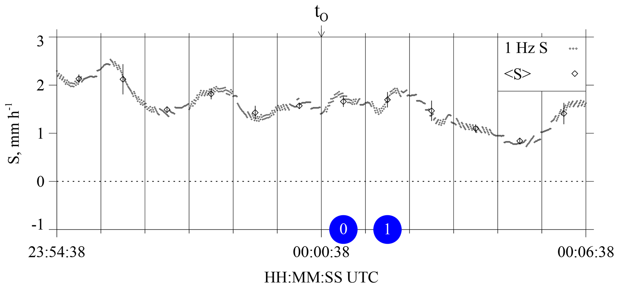
Figure 7 12 min of HP snowfall measurements from 14–15 December 2016. Gray dots are S values calculated using hotplate output recorded at 1 Hz. Black diamonds are the 1 min averaged values (± 1 standard deviation). The t₀ is shown above the panel, and blue circles designate the i=0 and i=1 HP averaging intervals.

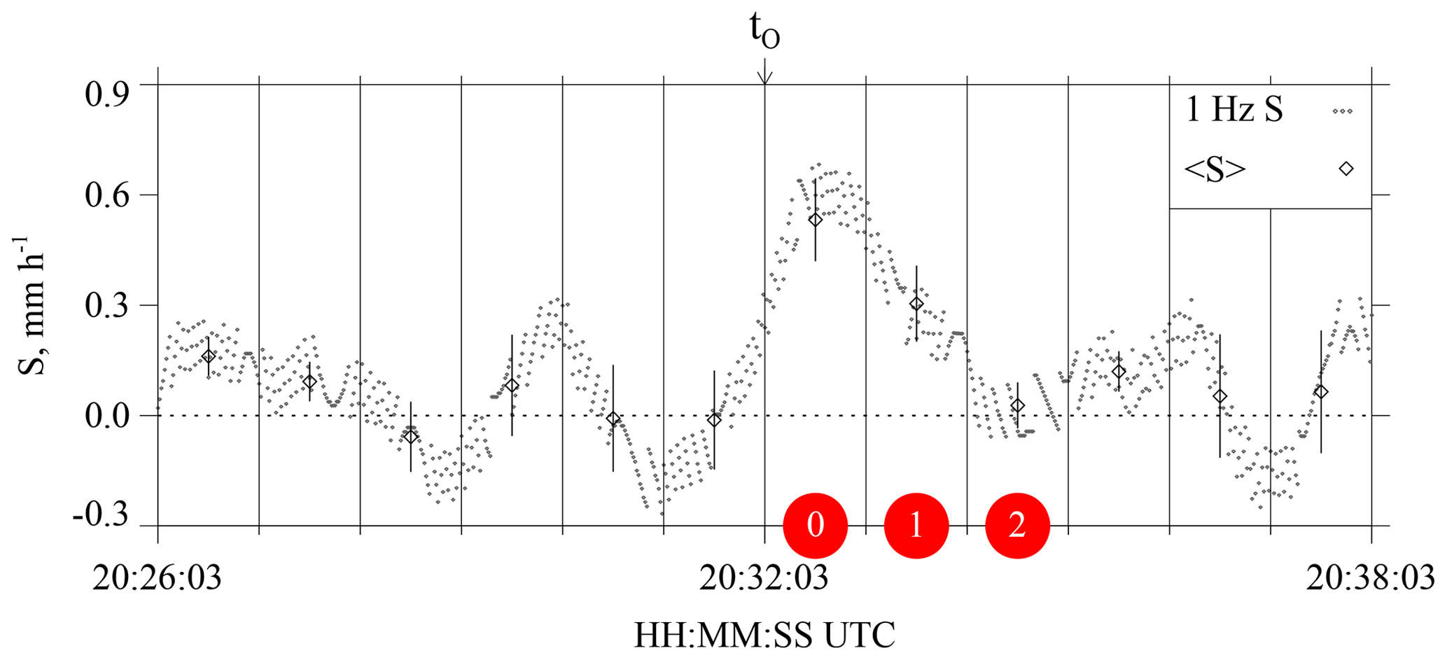
Figure 8 12 min of HP snowfall measurements from 3 January 2017. Gray dots are S values calculated using hotplate output recorded at 1 Hz. Black diamonds are the 1 min averaged values (± 1 standard deviation). The t₀ is shown above the panel, and red circles designate the i=0, i=1, and i=2 HP averaging intervals. The i=2 interval is a special case discussed at the end of Sect. 3.5.

Figures 9a–b and 10a–b have enlarged views of the altitude–time WCR cross sections recorded on the 2 flight days. Different from Fig. 5a and c, these measurements are only from the WCR's down-looking antenna. Additional differences are the following: (1) the plots are set up so that Z and V_D structures downwind of the hotplate can be seen. These structures are discussed in the following section. (2) The WCR measurements are shown for 50 s of flight. With the WKA ground speed approximately 125 m s⁻¹ (Table 3), the distance along the abscissa is 6250 m. (3) Colored circles that surround the indexes are placed below the WCR averaging domains. The latter are drawn with solid black lines and are seen to overlay both the Z and V_D altitude–time cross sections. Consistent with Fig. 6b and d and Appendix A, one of these black lines is vertical and another is negatively sloped. Figure 10a and b also have the i=2 domains discussed at the end of this section.

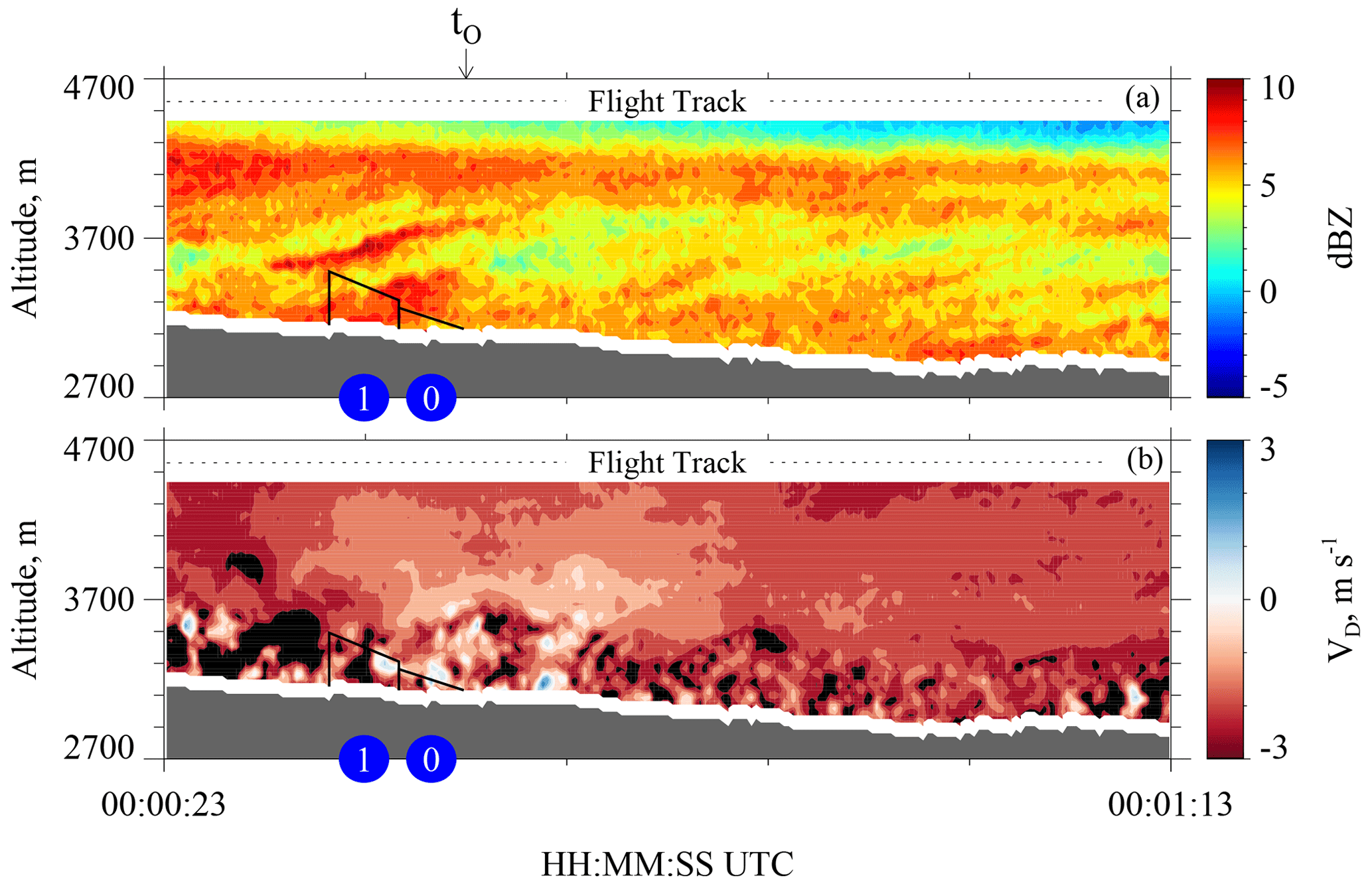
Figure 9 50 s of measurements from the down-looking WCR antenna on 15 December 2016. (a) Cross section of reflectivity t₀ − 15 s to t₀ + 35 s. (b) Cross section of Doppler velocity t₀ − 15 s to t₀ + 35 s. The t₀ is shown above the top panel. In both panels, the solid black lines (vertical and sloped) encompass the i=0 and i=1 WCR averaging domains, and blue circles designate the WCR averaging domains.

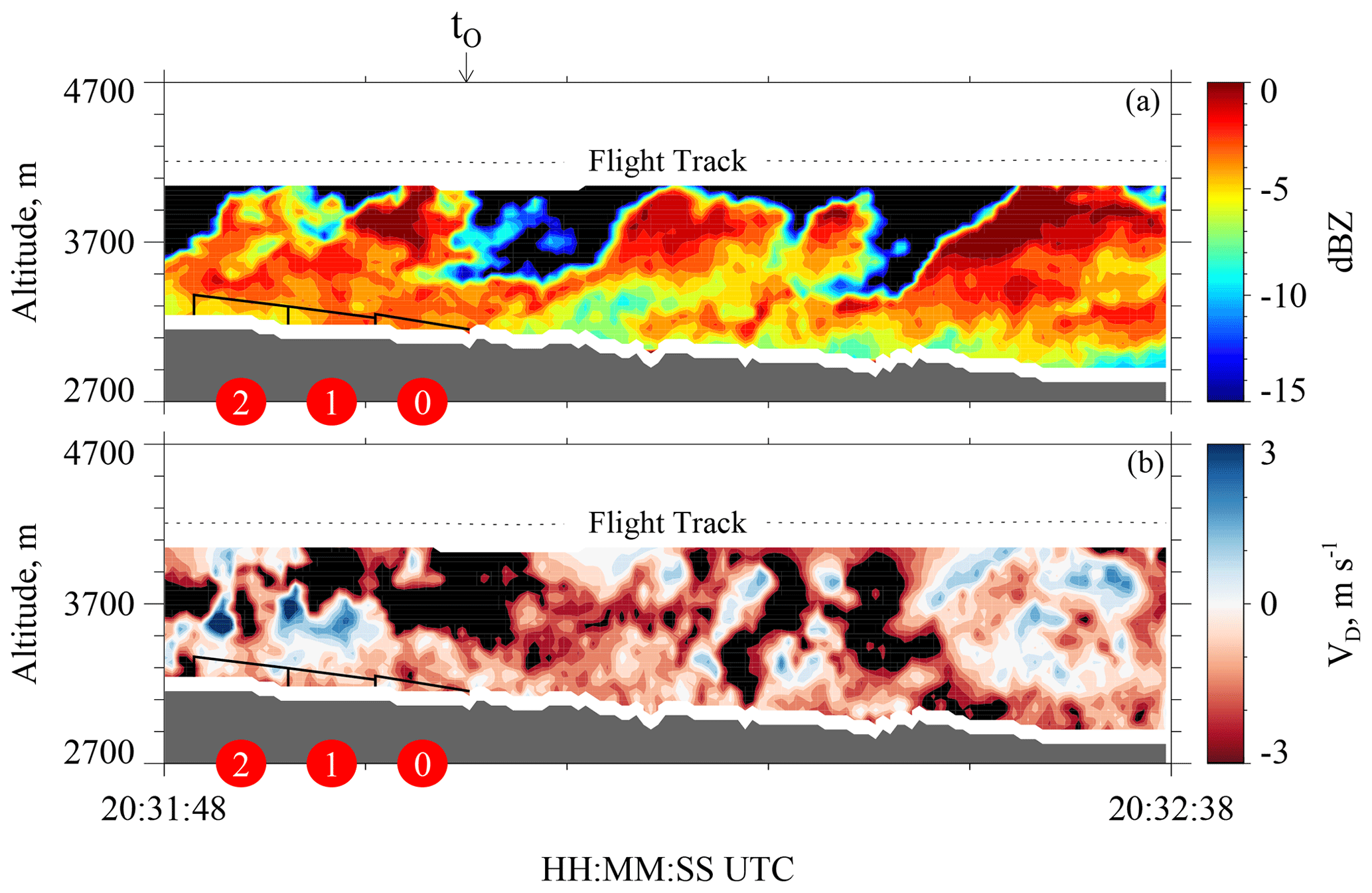
Figure 10 50 s of measurements from the down-looking WCR antenna on 3 January 2017. (a) Cross section of reflectivity t₀ − 15 s to t₀ + 35 s. (b) Cross section of Doppler velocity t₀ − 15 s to t₀ + 35 s. The t₀ is shown above the top panel. In both panels, the solid black lines (vertical and sloped) encompass the i=0, i=1, and i=2 WCR averaging domains, and red circles designate the i=0, i=1, and i=2 WCR averaging domains. The i=2 domain is a special case discussed at the end of Sect. 3.5.

The i=0 and i=1 averages of S and Z are presented in Table 6, and the corresponding averaging intervals are viewable in Figs. 7 and 9a (15 December 2016) and in Figs. 8 and 10a (3 January 2017). According to the averaging scheme (Fig. 6), the i=1 HP averaging interval is time-shifted positively compared to the i=0 HP averaging interval and the i=1 WCR averaging interval is time-shifted negatively compared to the i=0 WCR averaging interval. This arrangement of the averaging intervals is one way to average while also accounting for wind advection of the snow particles.

Table 6 Average wind measurements, average hotplate measurements, average WCR measurements, and attenuation-corrected reflectivities.

^a Horizontal wind advection speed (Eq. A7) calculated using values from the penultimate and last columns of Table 3. ^b 1 min average of the undercatch-corrected liquid-equivalent snowfall rate (± 1 standard deviation). An example averaging interval is the i=0 interval in Fig. 7. ^c Number of samples used to calculate the WCR statistics. The averaging domains (e.g., i=0 in Figs. 9a–b and 10a–b) encompass the WCR samples which are the basis for the WCR statistics presented in this table. ^d Average of Doppler velocity within the averaging domains. ^e Standard deviation of Doppler velocity within the averaging domains. ^f Maximum likely snow particle speed toward the ground (Eq. A8). ^g Average reflectivity (± 1 standard deviation). These values are not corrected for attenuation. ^h Attenuation-corrected reflectivities. These were derived using reflectivities from the penultimate column of this table, attenuations from Table 4, and Eq. (1).

As discussed earlier in this section, the averaging scheme initializes with 60 s blocks of HP data between t₀ and t₀ + 120 s. When we applied the scheme to data from 3 January 2017, but outside the specified time range, an inconsistency was documented. This is apparent in Fig. 8, where the t₀ + 120 s to t₀ + 180 s interval (i.e., the i=2 interval) has negligible average S, while in Fig. 10, the i=2 interval has a non-negligible average Z (∼ 0.3 mm⁶ m⁻³). A firm explanation is not available for the inconsistency, but a factor may be the convective nature of the fields in Fig. 10a and b. Because of the inconsistency, only averages corresponding to the i=0 and i=1 intervals are analyzed further.

3.6 Snow particle imagery

In Figs. 9a and 10a, the time for a snow particle to move the abscissa and ordinate distances is different. The ratio of these two times is 2.6. This follows from our choice of abscissa and ordinate ranges, from values of particle fall speed (1 m s⁻¹) and horizontal wind advection speed (8 m s⁻¹), which we assumed, and from the WKA ground speed (gs ∼ 125 m s⁻¹; Table 3). The assumed values are approximately consistent with values of 〈V_D〉 and v_w, in Table 6, and with the V_D sign convention (Sect. 2.3). We also used gs = 125 m s⁻¹ to scale (virtually) the time axes in Figs. 9a and 10a to a horizontal distance. Within the scaled coordinate frames, we assumed that all snow particle trajectories have negative slope ($\mathrm{\Delta }z/\mathrm{\Delta }x$ = −1 m s⁻¹/8 m s⁻¹ = −0.12) and that all trajectories are stationary. However, both assumptions seem inconsistent with the reflectivity structures in Fig. 5a where positively sloped particle fall streaks are evident at ∼ 5500 m, inconsistent with Fig. 9a where positively sloped fall streaks are at ∼ 3500 m, and inconsistent with the positively sloped fall streaks in Fig. 10a. On both flight days, the fall streaks evince particle sources that move horizontally and with a horizontal speed that is larger than the v_w = 8 m s⁻¹ applied in the estimate of the trajectory slope. It may be that the source's horizontal speed is comparable to the flight-level WKA-derived horizontal wind (27 to 32 m s⁻¹; Table 3), but we do not have data needed to verify that assertion. Based on the assumption that snow particles followed the fall streaks while both were advecting horizontally, we looked downwind of the hotplate – at a time later than t₀ in Figs. 9a and 10a – for particles that became those that produced snowfall at the hotplate.

Particle images from 15 December 2016 were analyzed using the 2DP. With this instrument the maximum all-in particle size (in the horizontal direction perpendicular to flight) is 6400 µm and the particle size resolution is 200 µm (Sect. 2.2). Within the time interval picked for this analysis (discussed below), particles in the smaller of the two spectral modes, with mode size ∼ 400 µm, were more numerous (results not shown). Because the 400 µm particles are poorly resolved by the 2DP, and the same can be said for somewhat larger particles, those smaller than 1000 µm were excluded from the following analysis. Figure 11a shows imagery from 12 s of measurements acquired near the end of the sequence in Fig. 9a (00:01:02 to 00:01:14 UTC). This time interval was selected by tracing forward from t₀, along the slope of the fall streaks, to the flight level. Many of the particles are rounded (indicating riming) and a few have arms, likely due to incomplete conversion of branched crystals to rimed snow particles. The mode size corresponding to these images is 1600 µm. No liquid water was detected with these particles (LWC < 0.01 × 10⁻³ kg m⁻³; Fuller, 2020; her Fig. 8), but liquid was detected at ∼ 00:00:00 UTC as the aircraft approached the ridgeline (Fig. 5a and b).

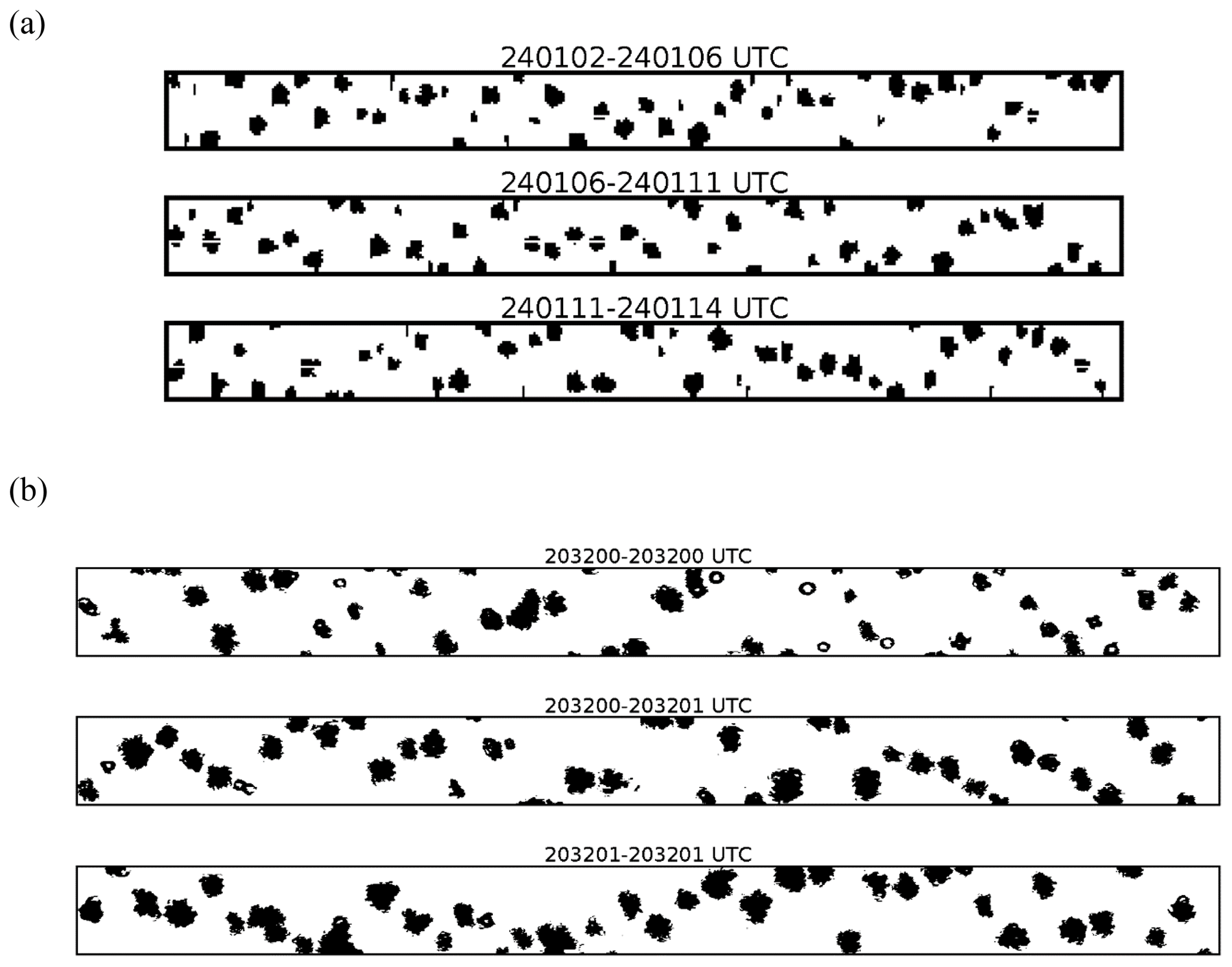
Figure 11 (a) 2DP particle imagery from 15 December 2016. The height of the strips is 6400 µm. These particles are estimated to be representative of those that fell from flight level toward the hotplate. (b) 2DS particle imagery from 3 January 2017. The height of the strips is 1280 µm. These particles are estimated to be representative of those that fell from flight level toward the hotplate.

Turning to imagery from 3 January 2017, the most appropriate location for analysis would be through the second billow structure evident in Fig. 10a (i.e., very close to the middle of the Fig. 10a sequence). This billow sourced a fall streak that terminated at the hotplate (i.e., at the time t₀ indicated in the figure). However, the aircraft only clipped the top of this billow, and it was only when sampling the billow seen ∼ 13 s earlier that larger ice particle concentrations (∼ 20 000 m⁻³) (Fuller, 2020; her Fig. 10) and larger LWC (∼ 0.08 × 10⁻³ kg m⁻³; Fig. 5d) were detected. Maximum reflectivities were the same in all three billows (Z ∼ 1 mm⁶ m⁻³; 0 dBZ), so it was assumed that imagery collected in the first billow (20:32:00 to 20:32:02 UTC) was representative of what was falling toward the hotplate. The 2DS was used to image these particles (Fig. 11b); with this instrument the maximum all-in particle size (in the horizontal direction perpendicular to flight) is 1280 µm and the size resolution is 10 µm (Sect. 2.2). Most of the objects in Fig. 11b appear to be rimed and their mode size is ∼ 400 µm. It is also noted that particles smaller than 100 µm were eliminated from these images; however, compared to the ∼ 400 µm particles those smaller than 100 µm were significantly less abundant (results not shown).

3.7 S–Z relationships

Our S–Z pairs are presented in Table 6 where the indexes (i=0 and i=1) are used to indicate results derived for the averaging intervals. In the penultimate column of Table 6, reflectivities are not corrected for attenuation; however, in the last column of Table 6 and in Fig. 12, the attenuation-corrected reflectivities are presented. Reflectivities from the penultimate column of Table 6, attenuations from Table 4, and Eq. (1) were used to calculate the corrected reflectivities. Also shown in Fig. 12 (black filled circles) is a subset of the S–Z pairs from PV11's Fig. 11 (0.01 < Z < 10 mm⁶ mm⁻³) and the PV11 best-fit line (black). Results from PV11 are specified as $S\left({\mathit{\rho }}_{\mathrm{1}}\right)/Z$ because those authors applied the lower of two density–size functions (ρ₁) and the lower of two fall speed–size functions with airborne measurements in calculations of snowfall rates (Sect. 1 and Table 1).

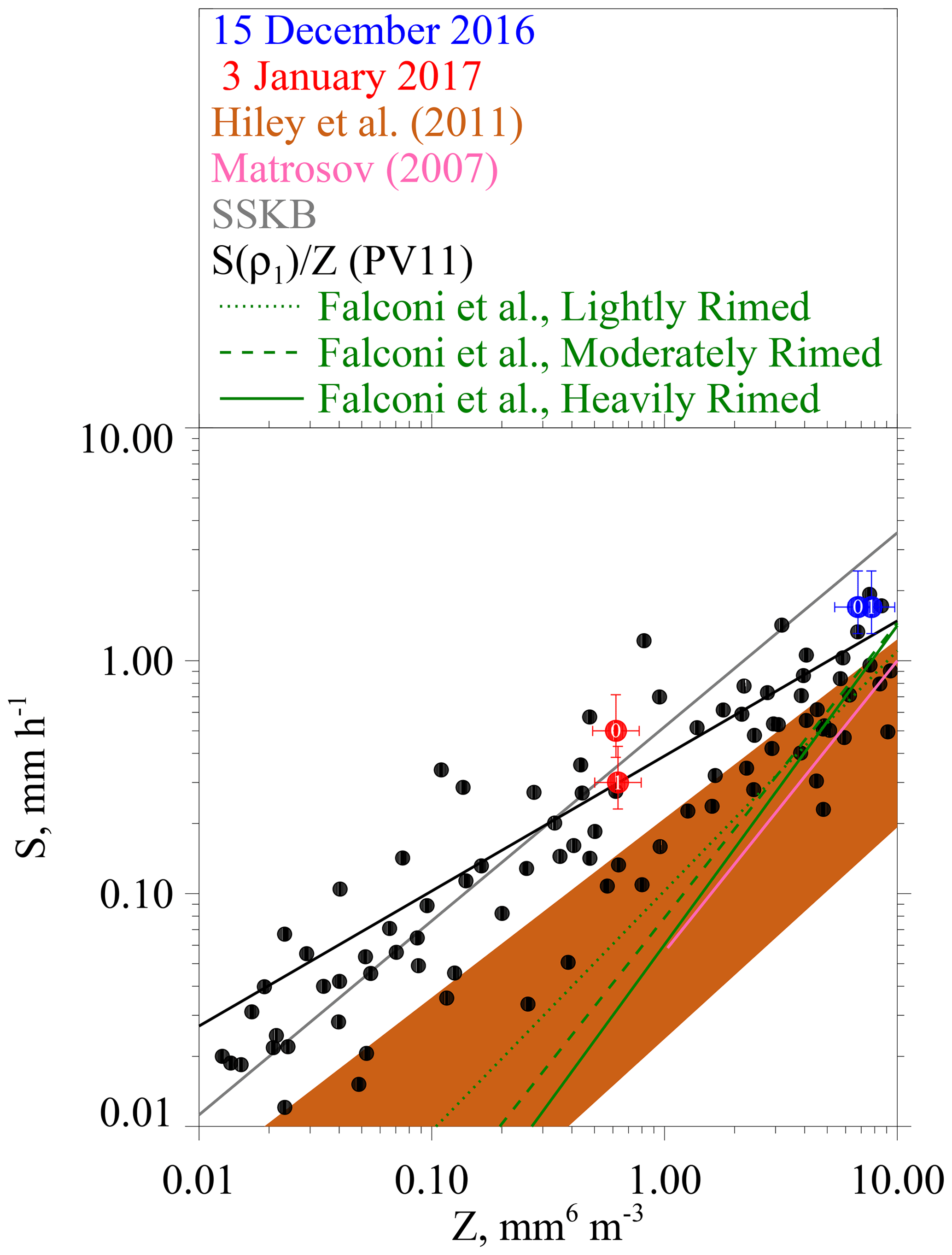
Figure 12 Snowfall rate versus radar reflectivity. Red and blue circles are plotted at attenuation-corrected reflectivities (Table 6) for the i=0 and i=1 averaging. Error bars on these points represent precisions of the reflectivity (Sect. 2.3) and snowfall rate (Sect. 2.4) measurements. Also plotted are the S–Z relationship lines from Sect. 1 and Table 1. These are the S–Z lines defining the swath of S–Z relationships from Hiley et al. (2011), the S–Z relationship from Matrosov (2007), the S–Z relationship abbreviated SSKB, PV11's best-fit line, and the S–Z relationships from Falconi et al. (2018) (their Table 2). The $S\left({\mathit{\rho }}_{\mathrm{1}}\right)/Z$ points (black filled circles) are a subset from PV11's Fig. 11 (0.01 < Z < 10 mm⁶ mm⁻³).

There are two potential biases in the values of snowfall rate we tabulate (Table 6) and plot (Fig. 12). First, the two snowfall events had flight-level vertical wind velocities (Fig. 5b and d) that were positive (upward) upwind of the ridgeline and the opposite downwind of the ridgeline. Except for the strongest downdraft on 3 January 2017, the magnitude of this variance is ∼ 1 m s⁻¹ (Fig. 5b and d). Assuming 1 m s⁻¹ was the downward wind immediately over the hotplate, the snow particles would have approached the HP gauge faster than their fall speed. Our basis for stating this is fall speeds for the mode sizes discussed in Sect. 3.6 (1600 and 400 µm) and our assumption that the particles were graupel. (Table 7 has these characteristic sizes and fall speeds.) However, the conjectured relative effect of a downward wind is likely an overestimate – because of divergence occurring as downward moving air approached the surface and because the sizes in Table 7 likely underestimate what fell to the hotplate. Relevant to the last of these assertions, we used the altitude, T, and RH measurements (Table 3) to calculate the vertical distance available for growth via riming, and thus for a fall speed increase, between the flight level and the lifted condensation level. Assuming an adiabatically stratified liquid cloud and unit collection efficiency (these assumptions overestimate growth by riming) as well as no change in particle cross section (underestimates growth by riming), our calculations indicate that relative increases in size and fall speed were 40 % and 20 %, respectively, on 3 January 2017 and that these relative increases were a factor of 2 larger on 15 December 2016.

Table 7 Estimates of snow particle fall speed.

Second, there is concern that values of S from 3 January 2017 are underestimated. Although values of S must be > 0, we presented 1 Hz values (gray points, Fig. 8) approaching −0.3 mm h⁻¹. Negative values resulted because we did not impose a threshold of 0 mm h⁻¹ on the uncorrected snowfall rates (this thresholding is discussed in Z18) and because negative snowfall rate values (uncorrected for catch inefficiency) are amplified by the gauge-catch correction (Sect. 2.4). The implication is that 0.2 mm h⁻¹ could be added to the 1 min averaged values of snowfall rate in Table 6 and in Fig. 12. Here, the assumption is that an averaged S of −0.2 mm h⁻¹, as in Fig. 8, indicates no snowfall at the hotplate; however, because the hotplate was operated autonomously (Sect. 2.1) we have no way to verify the assumption.

4 Results

Figure 12 shows our four snowfall rate–reflectivity pairs (red and blue circles) after the reflectivities were corrected for attenuation. The error bars on these data pairs represent the precision of the Z measurement (Sect. 2.3) and the precision of the S measurement (Sect. 2.4). Presentation clarity was what guided the selection of S and Z axis ranges in this figure but with the consequence that 32 of PV11's S–Z pairs are not shown because they plot at Z > 10 mm⁶ m⁻³. The way that the PV11 data pairs scatter closest to Z = 10 mm⁶ m⁻³, combined with the fact that the PV11 data pairs at Z > 10 mm⁶ m⁻³ are not shown, could lead to the interpretation that the slope describing the best-fit relationship at Z approximately > 2 mm⁶ m⁻³ should be decreased relative to the actual slope of the PV11 best-fit line. Readers who view PV11's Fig. 11 will conclude that this interpretation is not warranted.

As discussed in Sect. 1, computation-based S–Z relationships have inputs from parameterized descriptions of density, shape, fall speed, PSD, and particle size. The computation-based S–Z relationships are in the top three rows of Table 1; the subsequent two rows of the table have S–Z relationships that resulted from a hybridization of measurements and calculations (PV11 and Falconi et al., 2018).

We now compare our snowfall rates (fourth column of Table 6) to snowfall rates where they plot on an S–Z relationship line evaluated at our attenuation-corrected reflectivities. The departure between these is reported as a relative S difference expressed as $\mathrm{|}(S_{\text{HP}}-S)\mathrm{|}/S$, where S_HP is from Table 6 and where S is on an S–Z relationship line. All possible comparisons are presented graphically in Fig. 12. Table 1 has both the minimum relative S differences and the salient maximum relative S differences. The comparisons will be discussed in the order of presentation in Table 1.

In comparisons of our snowfall rates and the upper-limit S–Z relationship line from Hiley et al. (2011) the relative difference is no smaller than 0.7 and 1.0 on 15 December and 3 January, respectively. These minimum relative differences exceed the hotplate precision (Sect. 2.4) by at least a factor of 2. It is concluded that our paired values of undercatch-corrected precipitation rate and attenuation-corrected radar reflectivity provide evidence that a calculation of S based on the Hiley et al. (2011) upper limit, when applied to rimed snow particles, is associated with a low-biased estimate of S. A retrieval based on the Hiley et al. average S–Z relationship (not shown), which bisects the orange region in Fig. 12, corresponds to an even larger low bias. This is a concern because Hiley et al. (2011) used their average S–Z relationship to retrieve global snowfall distributions and since global observations reported in Wang et al. (2013) document the frequent occurrence of supercooled liquid within snowing clouds.

Figure 12 shows the separation between our measurements and the Matrosov (2007) calculation. The separation is about a factor of 2 (minimum relative difference of 1.4) for the points obtained on 15 December 2016 and corresponds to an underestimation of S (low bias) when compared to our measurements. The points from 3 January 2017 plot at an attenuation-corrected reflectivity smaller than the lower limit of the calculation (Matrosov, 2007). Since the particle images (Fig. 11a and b) reveal no evidence of the particle type modeled by Matrosov (2007) (aggregates), it is not surprising that the Matrosov S–Z relationship is not representative of our measurements.

One plausible reason for the low bias discussed in the previous two paragraphs is the smaller density implicit in most computationally based S–Z relationships, especially those which assume that snow particles are crystals. Densities are quite different for crystals versus those for rimed snow particles. For example, in Brown and Francis (1995), assuming a 2 mm crystal, the density is ∼ 30 kg m⁻³, whereas in PV11 (their Eq. 1), assuming a 2 mm graupel particle, the density is ∼ 200 kg m⁻³. Because aggregates are collections of crystals, this comparison of crystal and graupel densities also seems relevant to a comparison of graupel and aggregate snow particle densities.

Figure 12 compares our S_HP–Z^′ data pairs to the SSKB S–Z relationship line, and Table 1 presents the relative differences between the data pairs and the SSKB line. Compared to the S–Z relationship represented by the top of the orange region in Fig. 12 and compared to the Matrosov (2007) relationship, the SSKB line plots closer to our data points (minimum relative difference ∼ 0.3). We note that the only instances of S_HP < S are three of four comparisons of our measurements to the SSKB relationship. A possible reason for this is that the density applied in SSKB (Table 1) is not entirely representative of conditions during our study. An analysis of the sensitivity of the SSKB to a change in density is needed to investigate our assertion.

Comparisons of our S_HP–Z^′ data pairs and PV11's best-fit line are also in Table 1. The table demonstrates that the agreement is reasonable – with a minimum relative difference no larger than 0.3 – and Fig. 12 shows that our data pairs plot at or above the PV11 best-fit line.

Based on data from PV11 and our S_HP–Z^′ data pairs, as well as the S–Z relationship abbreviated SSKB, it is expected that the S–Z relationships reported by Falconi et al. (2018) for rimed snow particles (Sect. 1) would plot higher in S-versus-Z space than is illustrated in Fig. 12. Notably, only the upper end of the Falconi et al. lines (i.e., at Z > 8 mm⁶ m⁻³) plot above the upper limit that Hiley et al. (2011) developed for unrimed snow particles. A plausible explanation for the lower-than-expected S–Z relationships of Falconi et al. is now offered. Falconi et al. used liquid water path as a proxy for the extent of snow particle riming (von Lerber et al., 2017). A consequence may have been that the proxy did not dependably exclude unrimed snow particles (crystals and aggregates) from the riming categories of Falconi et al. If this was the case, then the data groupings that were the basis for the Falconi et al. S–Z relationships may have been affected. When comparing the heavily rimed S–Z relationship of Falconi et al. to our S_HP–Z^′ data pairs we find that the minimum relative differences are 0.6 (15 December) and 8.5 (3 January) (Table 1). Additionally, the differences are 0.5 (15 December) and 5.9 (3 January) when applying the moderately rimed S–Z relationship of Falconi et al. (results not shown). Further research is needed to resolve the reason for the mismatch between the snowfall rate–reflectivity pairs reported here and the S–Z relationships reported in Falconi et al.

Our conclusion that the upper-limit S–Z relationship from Hiley et al. (2011) underestimates S would be modified if our WCR-derived reflectivities were negatively biased. Assuming the reflectivities are negatively biased by 2.5 dBZ, the minimum relative differences discussed previously change to 0.1 and 0.3 on 15 December and 3 January, respectively. A bias in reflectivity of this magnitude cannot be ruled out but neither can a positive bias of the same magnitude (Sect. 2.3). The latter increases the minimum relative differences to 1.6 and 2.2 on 15 December and 3 January, respectively. In each of these calculations we have summed the attenuations (Table 4) with ± 2.5 dBZ and used Eq. (1) to calculate error-perturbed reflectivities.

The scatter of measurements in Fig. 12, the plausibility of a −2.5 to +2.5 dBZ bias in WCR reflectivity measurements, and error in measurement of S (Sect. 2.4) indicate that refined techniques will be needed in future investigations which apply the approach described here. Taking into consideration the goal of evaluating snowfall rates from space, some advance in satellite remote sensing also seems warranted. One issue is diagnosing where riming is occurring within clouds. Both lidars and radiometers can sense supercooled liquid water from space (e.g., Battaglia and Panegrossi, 2020) and, if combined with Doppler radars operating at multiple wavelengths, can diagnose the presence of rimed precipitation particles. Despite limitations of the multiple-wavelength Doppler method in scenarios with vertical air speed comparable to and larger than particle fall speed (Vogl et al., 2022), the method has been validated in ground-based field studies (Kneifel et al., 2015; Mason et al., 2018). Technical challenges also remain for implementing the method from space (Battaglia et al., 2020).

5 Conclusions

We have reported surface measurements of S and near-surface measurements of Z. The latter came from overflights of a ground site, where a precipitation gauge was operated, and were acquired using an airborne W-band radar. The values of Z were corrected for attenuation.

The reported S_HP–Z^′ pairs plot at or above the S-versus-Z best-fit line of PV11 (Fig. 12) and the minimum relative S difference (Table 1) is no larger than 0.3. The PV11 data came from airborne measurements of W-band reflectivity, acquired within ± 100 m of flight level, and from coincident measurements of snow particle imagery. PV11 used a density–size function, a fall speed–size function, and measurements (PSD and particle images) to calculate S for snow particles that were classified as both rimed crystals and graupel. This classification is consistent with the particle imagery we have presented (Fig. 11).

We have documented a substantial difference in comparisons between our snowfall rate measurements and reflectivity-dependent snowfall rates calculated using an upper-limit S–Z relationship (Hiley et al., 2011). This S–Z relationship produces an underestimate of the snowfall rate (Fig. 12) when compared to our measurements. We also report substantial snowfall rate underestimates in comparisons of our measurements to the S–Z relationship developed by Matrosov (2007). The underestimates obtained using the Hiley et al. and Matrosov S–Z relationships are perhaps expected given that the density factored into those S–Z calculations is small compared to that for rimed snow particles. It is also expected that the larger density and spherical shape applied in the SSKB S–Z relationship contributed to the better agreement seen in the comparison of the SSKB relationship to our snowfall rate measurements. Our conclusion is that some snowfall retrievals (e.g., Hiley et al., 2011) will underestimate S for weather targets containing rimed snow particles. Additionally, we report findings at odds with the measurements and analysis of Falconi et al. (2018). Those researchers reported S–Z relationships for rimed snow particles which in instances with Z < 8 mm⁶ m⁻³ plot below the upper limit of Hiley et al. (Fig. 12). A consequence is that the minimum relative S differences in our comparison to Falconi et al. (assuming the Falconi et al. heavily rimed classification) are comparable to and larger than in our comparison to the Hiley et al. upper-limit S–Z relationship (Table 1).

New research is needed to refine the S–Z relationship for rimed snow particles. This could be computational – e.g., investigation of the utility of parameterizing S in terms of both Z and density – or could be observational. Unlike the investigation of PV11, where only an airborne platform was employed, we have demonstrated that useful information can be obtained using coordinated ground-based and airborne systems. Provided all key measurements are acquired (S, PSD, particle imagery, and Z), another approach would be with only ground-based instrumentation. This would avoid some of the complications encountered in this study, including W-band attenuation and a reliance on particle imagery acquired aloft. A study with both ground-based and airborne systems would also be useful for understanding an S–Z mismatch apparent at Z < 8 mm⁶ m⁻³. Elements of the mismatch are the measurements reported here, PV11's best-fit line, and the measurement-based S–Z relationships reported by Falconi et al. (2018). These three research teams reported measurements relevant to the development of an S–Z relationship for rimed snow particles.

Appendix A

This Appendix explains how HP (hotplate) and WCR (Wyoming Cloud Radar) averages were evaluated. The scheme starts with an HP averaging interval (duration 60 s) and derives a WCR averaging interval and a WCR averaging domain. The latter encompasses a subset of the altitude–time cross section sampled by the WCR. The top boundary of the domain was derived using vertical-component Doppler velocities within the domain. Because of this dependence, the line defining the top boundary was derived iteratively.

With the overflight time symbolized by t₀, the beginning and ending times of the first HP averaging interval are

$$\begin{array}{}\text{(A1)}& {\displaystyle }{t}_{\text{HP,B}}=t_{\mathrm{0}},\text{(A2)}& {\displaystyle }{t}_{\text{HP,E}}=t_{\mathrm{0}}+\mathrm{60}.\end{array}$$

Since two adjacent HP averaging intervals are evaluated in this analysis, we express the averaging times with the following recursive equations:

$$\begin{array}{}\text{(A3)}& t_{\text{HP,B}}\left(i\right)=t_{\mathrm{0}}+i\cdot \mathrm{60}\end{array}$$

and

$$\begin{array}{}\text{(A4)}& t_{\text{HP,E}}\left(i\right)=t_{\mathrm{0}}+(i+\mathrm{1})\cdot \mathrm{60}.\end{array}$$

In Eqs. (A3) and (A4) the index is $i\in \mathit{\{}\mathrm{0},\mathrm{1}\mathit{\}}$. A special case with i = 2 is also analyzed (Sect. 3.5). Analogous to the recursion in Eq. (A4), the ending time of a WCR averaging interval is

$$\begin{array}{}\text{(A5)}& t_{\text{WCR,E}}\left(i\right)=t_{\mathrm{0}}-i\cdot \mathrm{60}\cdot v_{\mathrm{w}}/\mathrm{gs}.\end{array}$$

Here v_w is a wind advection speed (discussed below) and the second term on the right-hand side is a wind advection distance divided by the WKA (Wyoming King Air) ground speed (gs). Analogous to Eq. (A5), the beginning time of a WCR averaging interval is

$$\begin{array}{}\text{(A6)}& t_{\text{WCR,B}}\left(i\right)=t_{\text{WCR,E}}-(i+\mathrm{1})\cdot \mathrm{60}\cdot v_{\mathrm{w}}/\mathrm{gs}.\end{array}$$

The wind advection speed (v_w) in Eqs. (A5) and (A6) was calculated using an altitude-dependent west-to-east wind velocity (u) and an altitude-dependent south-to-north wind velocity (v). These altitude-dependent component velocities were calculated using the horizontal wind vectors in the penultimate and last columns of Table 3. Plots of the component velocities versus altitude and the linear functions used to relate component velocities to altitude are presented in Fig. A1a and b.

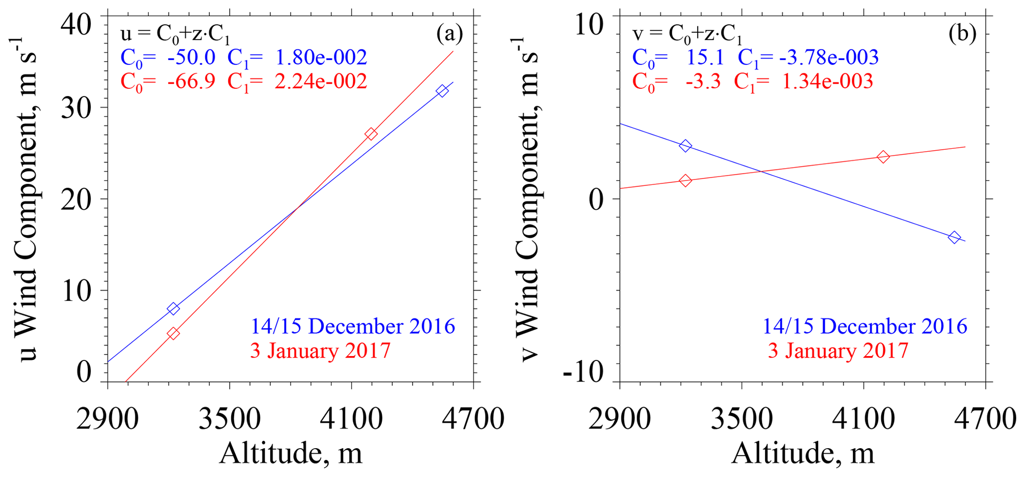
Figure A1 (a) West-to-east (u) wind velocity derived using measurements from the WKA and the AmeriFlux (AF) tower. Also shown is the linear function used to relate u to altitude. (b) South-to-north (v) wind velocity derived using measurements from the WKA and AF. Also shown is the linear function used to relate v to altitude. WKA and AF velocities are presented as vectors in the penultimate and last columns of Table 3.

An altitude (z^′ = 3400 m) was assumed for evaluating the horizontal wind advection vector. This is the altitude of the ridges west and northwest of the HP site (Fig. 3a and b).

The WKA track vector (Table 3) defines the vertical plane of the WCR measurements. We assumed that wind advection of snow particles occurred parallel to this vector. With the assumption stated in the previous paragraph, the horizontal wind advection speed (v_w) was calculated as the projection of the horizontal wind vector onto the track vector.

$$\begin{array}{}\text{(A7)}& v_{\mathrm{w}}={\displaystyle \frac{u\left(z^{\prime }\right)\cdot {\mathrm{gs}}_x+v\left(z^{\prime }\right)\cdot {\mathrm{gs}}_y}{{\left({\mathrm{gs}}_x^{\mathrm{2}}+{\mathrm{gs}}_y^{\mathrm{2}}\right)}^{\mathrm{1}/\mathrm{2}}}}\end{array}$$

In Eq. (A7) the west-to-east and south-to-north components of the track vector are symbolized by gs_x and gs_y. Vector representations of the track vector are in Table 3. On 14–15 December 2016 and 3 January 2017, the values of v_w were 7.4 and 8.9 m s⁻¹, respectively.

In addition to the properties gs and v_w used to evaluate Eqs. (A5) and (A6), a WCR averaging domain was evaluated using a snow particle downward speed (Eq. A8).

$$\begin{array}{}\text{(A8)}& v_{\mathrm{p}}=\mathrm{|}\langle V_{\mathrm{D}}\rangle \mathrm{|}+{\mathit{\sigma }}_{V_{\mathrm{D}}}\end{array}$$

Here, 〈V_D〉 is the average of Doppler velocities within an averaging domain, |〈V_D〉| is the absolute value of the average, and ${\mathit{\sigma }}_{V_{\mathrm{D}}}$is the standard deviation of the average. On both the left-hand and right-hand side of Eq. (A8), all terms are greater than zero.

We interpret v_p as the maximum likely snow particle speed toward the ground. There are three reasons for this: (1) for the WCR averaging domains we analyzed, values of 〈V_D〉 were consistently less than zero (Table 6). This indicates that snow particles (on average) were moving toward the ground. (2) Again, for the WCR averaging domains we analyzed, ${\mathit{\sigma }}_{V_{\mathrm{D}}}$ was comparable to |〈V_D〉|. This indicates that turbulent eddies transported snow particles upward and downward at a speed comparable to their downward speed in still air. (3) The V_D values are reflectivity weighted (Haimov and Rodi, 2013) and are thus indicative of the motion of the largest particles within an averaging domain.

We now focus on the top boundary of a WCR averaging domain. Figure 6b and d have representations of the boundary. The slope defining this boundary was calculated as $-v_{\mathrm{p}}\cdot \mathrm{gs}/v_{\mathrm{w}}$. That is, particles below this boundary moved downward sufficiently fast and horizontally sufficiently slow to advect reasonably close to the hotplate. Starting with diagnosed values of gs and v_w, the values of v_p and slope were derived iteratively. The precision of the derived v_p is ± 0.1 m s⁻¹.