Highly resolved mapping of NO₂ vertical column densities from GeoTASO measurements over a megacity and industrial area during the KORUS-AQ campaign

The Korea–United States Air Quality (KORUS-AQ) campaign is a joint study between the United States National Aeronautics and Space Administration (NASA) and the South Korea National Institute of Environmental Research (NIER) to monitor megacity and transboundary air pollution around the Korean Peninsula using airborne and ground-based measurements. Here, tropospheric nitrogen dioxide (NO₂) slant column density (SCD) measurements were retrieved from Geostationary Trace and Aerosol Sensor Optimization (GeoTASO) L1B data during the KORUS-AQ campaign (2 May to 10 June 2016). The retrieved SCDs were converted to tropospheric vertical column densities using the air mass factor (AMF) obtained from a radiative transfer calculation with trace gas profiles and aerosol property inputs simulated with the Community Multiscale Air Quality (CMAQ) model and surface reflectance data obtained from the Moderate Resolution Imaging Spectroradiometer (MODIS). For the first time, we examine highly resolved (250 m × 250 m resolution) tropospheric NO₂ over the Seoul and Busan metropolitan regions and the industrial region of Anmyeon. We reveal that the maximum NO₂ vertical column densities (VCDs) were 4.94×10¹⁶ and 1.46×10¹⁷ molec. cm⁻² at 09:00 and 15:00 LT over Seoul, respectively, 6.86×10¹⁶ and 4.89×10¹⁶ molec. cm⁻² in the morning and afternoon over Busan, respectively, and 1.64×10¹⁶ molec. cm⁻² over Anmyeon. The VCDs retrieved from the GeoTASO airborne instrument were correlated with those obtained from the Ozone Monitoring Instrument (OMI) (r=0.48), NASA's Pandora Spectrometer System (r=0.91), and NO₂ mixing ratios obtained from in situ measurements (r=0.07 in the morning, r=0.26 in the afternoon over the Seoul, and r>0.56 over Busan). Based on our results, GeoTASO is useful for identifying NO₂ hotspots and their spatial distribution in highly populated cities and industrial areas.

1 Introduction

Nitrogen dioxide (NO₂) is one of the most important atmospheric trace gases and plays a key role in aerosol production and tropospheric ozone photochemistry (Boersma et al., 2004; Richter et al., 2005). Furthermore, high concentrations of NO₂ in the atmosphere have adverse effects on human health, such as respiratory infections and associated symptoms (Brauer et al., 2002; Latza et al., 2009).

The main sources of NO₂ in the atmosphere are fossil fuel combustion from vehicles and thermal power plants, lightning, and biogenic soil processes. Furthermore, NO₂ concentrations are highly correlated with population size (Lamsal et al., 2013). The implementation of emission control technology and environmental regulation has led to a decrease in surface NO₂ concentrations in western Europe, the United States, and Japan in the last few decades (Richter et al., 2005). The concentration of NO₂ in major metropolitan cities in South Korea and China is over 3 times larger than over similarly sized cities in Europe and the United States, despite NO₂ concentrations decreasing in China and South Korea (de Foy et al., 2016; Choo et al., 2020).

To date, several low-orbit spaceborne sensors, such as the Global Ozone Monitoring Experiment (GOME) (Burrows et al., 1999), the Scanning Imaging Spectrometer for Atmospheric Cartography (SCIAMACHY) (Burrows et al., 1995), the Ozone Monitoring Instrument (OMI) (Levelt et al., 2006), GOME-2 (Callies et al., 2000), and the Tropospheric Monitoring Instrument (TROPOMI) (Veefkind et al., 2012), have monitored atmospheric ozone and its precursors, including NO₂ and formaldehyde (HCHO) as a proxy for volatile organic compounds (VOCs). Furthermore, the Geostationary Environment Monitoring Spectrometer (GEMS) (Choi et al., 2018; Kim et al., 2020), which was launched on 18 February 2020, will form a constellation of geostationary satellites, including the upcoming Tropospheric Emission: Monitoring of Pollution (TEMPO) (Zoogman et al., 2017) and Sentinel-4 platforms, to continuously observe the air quality of the Northern Hemisphere during the day.

NO₂ retrievals from spaceborne hyperspectral measurements are typically conducted using the differential optical absorption spectroscopy (DOAS) method (Platt and Stutz, 2008) to first retrieve the view-dependent slant column density (SCD), and then radiative transfer models are used to determine the vertical column density (VCD) using an air mass factor (AMF) correction. Previous and ongoing spaceborne instruments use various radiative transfer codes and model input assumptions to calculate NO₂ AMF values at coarse spatial resolution. Because AMF weighting has a large impact on NO₂ retrievals using the DOAS method, it is important to use model input assumptions that most accurately match viewing and atmospheric conditions. Several studies have demonstrated the sensitivity of AMF calculations to inaccurate model input parameters (e.g., a priori NO₂ vertical profile and aerosol properties) and a priori data (cloud information and surface reflectance) (Leitão et al., 2010; Hong et al., 2017; Lorente et al., 2017; Boersma et al., 2018). NO₂ retrievals have also been consistently conducted based on surface remote sensing measurements, including the Multi-Axis DOAS (MAX-DOAS), Système D'Analyse par Observations Zènithales (SAOZ) spectrometer (Pastel et al., 2014), and Pandora (Herman et al., 2009) systems. These ground-based measurements can be used as validation references for both airborne and spaceborne measurements.

NO₂ retrievals from airborne remote sensing instruments, such as the Geostationary Coast and Air Pollution Event (GEO-CAPE) Airborne Simulator (GCAS) (Kowalewski and Janz, 2014), the Heidelberg Airborne Imaging DOAS Instrument (HAIDI) (General et al., 2014), the Geostationary Trace gas and Aerosol Sensor Optimization (GeoTASO) (Leitch et al., 2014), the Airborne Prism Experiment (APEX; Popp et al., 2012), the Airborne Imaging DOAS instrument for Measurements of Atmospheric Pollution (AirMAP; Meier et al., 2017; Schönhardt et al., 2015), the Small Whiskbroom Imager for atmospheric compositioN monitorinG (SWING; Merlaud et al., 2018), and the Spectrolite Breadboard Instrument (SBI; Vlemmix et al., 2017; Tack et al., 2019), have also been performed to identify local emission sources and obtain highly resolved horizontal NO₂ distributions.

Observations using airborne measurements have an advantage as they enable the observation of horizontal distributions of trace gases at resolutions higher than those of space-based satellites and provide data over a wider area than those of ground-based observations. For example, Nowlan et al. (2018) retrieved tropospheric NO₂ VCDs over Houston, Texas, during the Deriving Information on Surface Conditions from Column and Vertically Resolved Observations Relevant to Air Quality (DISCOVER-AQ) campaign and identified a high correlation with data retrieved from Pandora. Popp et al. (2012) also presented the morning and afternoon NO₂ spatial distribution in Zurich, Switzerland, using APEX. Tack et al. (2017) have conducted high-resolution mapping of NO₂ over three Belgium cities (Antwerp, Brussels, and Liège) using APEX, and Judd et al. (2020) and Tack et al. (2021) compared NO₂ VCDs retrieved from GCAS/GeoTASO and APEX with those obtained from TROPOMI over New York City and over Antwerp and Brussels, respectively. Merlaud et al. (2013) observed NO₂ VCDs in Turceni over Romania using SWING mounted on an uncrewed aerial vehicle (UAV) during the Airborne Romanian Measurements of Aerosols and Trace gases (AROMAT) campaign. These existing NO₂ retrievals using airborne measurements have been useful in constraining regional air quality models due to the highly resolved source identification and the ability to tie these results to ground-based observations.

This work focuses on airborne NO₂ retrievals from GeoTASO. This instrument was developed by Ball Aerospace to reduce mission risk for UV-Vis air quality measurements from geostationary orbit for the GEMS and TEMPO missions (Leitch et al., 2014). The retrieval of NO₂, SO₂, and HCHO observed from GeoTASO L1B data using DOAS and principal component analysis (PCA) (Wold et al., 1987) was conducted through the DISCOVER-AQ and Korea–United States Air Quality (KORUS-AQ) campaigns (Nowlan et al., 2016; Judd et al., 2018; Choi et al., 2020; Chong et al., 2020). The KORUS-AQ campaign was a joint study organized from May to June 2016 between the National Institute of Environmental Research (NIER) and National Aeronautics and Space Administration (NASA) to monitor megacity air pollution and transboundary pollution and to prepare for geostationary satellite (i.e., GEMS, TEMPO, and Sentinel-4) air quality observability (of trace gases and aerosols).

Although surface NO₂ concentrations in South Korea are the high due to high population density, high traffic volumes, and many industrial complexes and thermal power plants, and although NO₂ retrieval studies using airborne and ground measurements in North America, Europe, China, and Japan exist, data for South Korea remain limited. The specific objectives of this study are as follows: to retrieve tropospheric NO₂ vertical column data using GeoTASO measurements over polluted regions of the Seoul and Busan metropolitan areas and the Anmyeon industrial region of the Korean Peninsula; to estimate NO₂ VCD uncertainties using error propagation accounting for spectral fitting errors and AMF uncertainties associated with input data errors, including aerosol optical depth (AOD), single scattering albedo (SSA), aerosol peak height (APH), and surface reflectance (SR); and to compare NO₂ VCDs retrieved from GeoTASO and those obtained from OMI and ground-based Pandora instruments, as well as surface in situ measurements.

2 KORUS-AQ campaign area, measurements, and model simulation

2.1 Campaign area

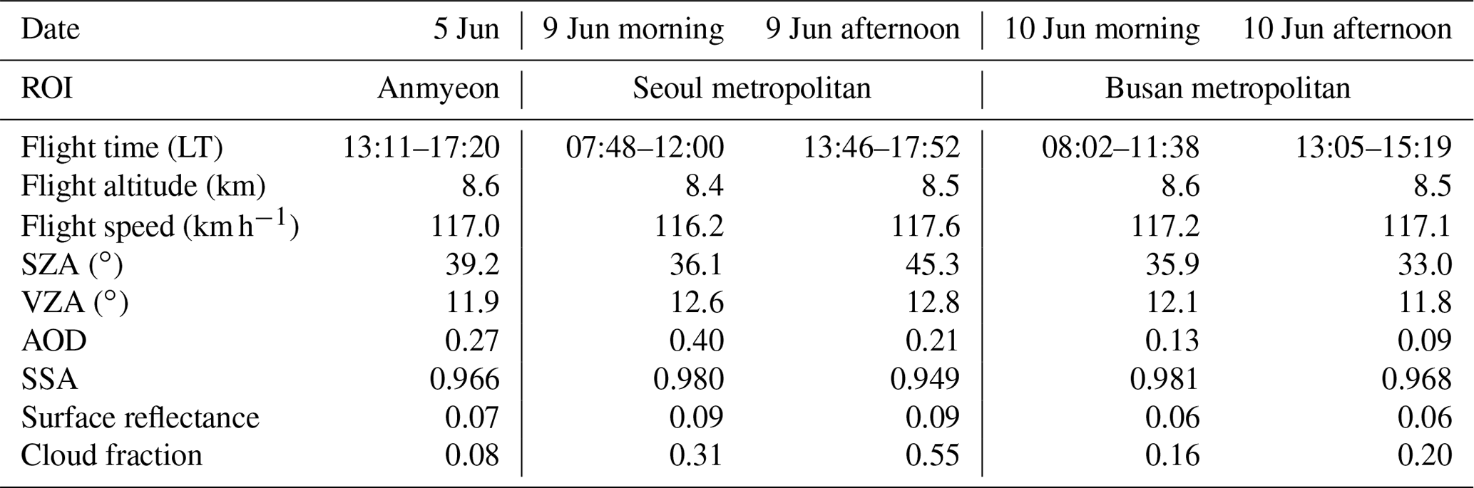
The Korean Peninsula, located on the Asia-Pacific coast, has a complex atmospheric environment due to local emissions and long-range transport under appropriate weather conditions (Jeong et al., 2017; NIER and NASA, 2020; Choo et al., 2020). Seoul, the capital of South Korea, and its metropolitan area are densely populated, while power plants and industrial activities on the northwestern coast emit relatively large amounts of pollutants. The KORUS-AQ campaign conducted three-dimensional observations, including ground-based remote, aircraft, and satellite observations, and air quality modeling to understand the complex air quality and interpret the observations of GEMS launched in 2020. The KORUS-AQ campaign period was from 2 May to 10 June 2016. During the KORUS-AQ campaign, air pollutants were conducted using the GeoTASO on board the NASA Langley Research Center B200 aircraft to monitor air quality and long-range transport of pollutants over the Korean Peninsula (NIER and NASA, 2020). The GeoTASO observations were conducted 30 times in 23 d out of 40 d. Most observations were made once or twice a day. Each flight was planned and conducted on a day when the weather conditions were fine and flight hours were approximately 2–4 h. We show the average values of GeoTASO flight information, such as flight time, altitude, speed, solar zenith angle (SZA), and viewing zenith angle (VZA) for the dates retrieved for NO₂ VCD; aerosol properties (AOD, SSA) extracted from the Community Multiscale Air Quality (CMAQ) model; and cloud fraction and SR extracted from the Moderate Resolution Imaging Spectroradiometer (MODIS) in Table 1. Flight information about the date of the aircraft observation can be found at http://www-air.larc.nasa.gov/missions/korus-aq/docs/KORUS-AQ_Flight_Summaries_ID122.pdf (last access: 26 October 2022). Figure 1 indicates the flight routes of B200 and the tropospheric NO₂ VCD obtained from the OMI during the campaign period. The observations were concentrated in the metropolitan areas of Seoul and Busan and the industrial area of Anmyeon, with an average flight altitude of ∼8.5 km during KORUS-AQ.

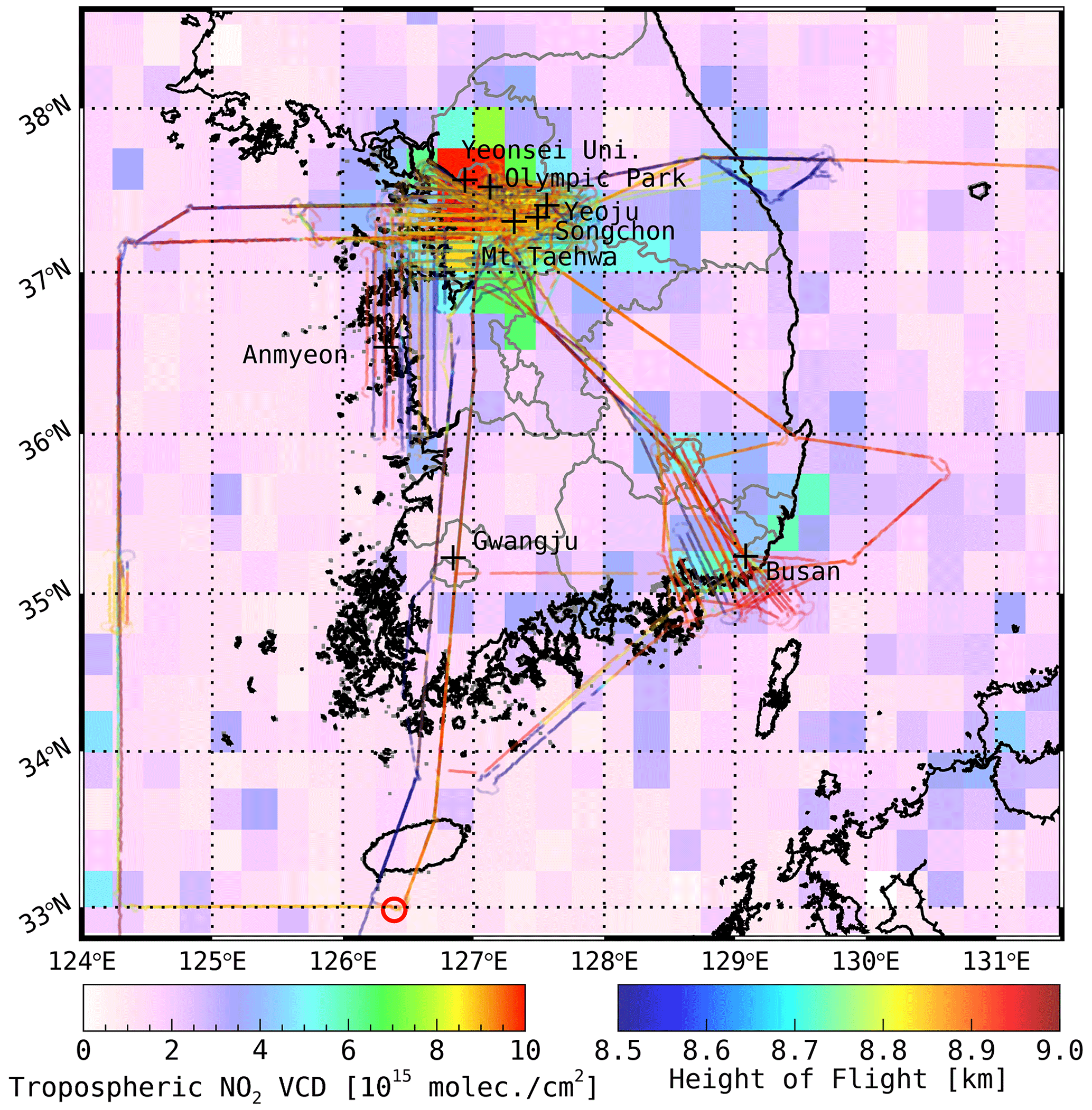
Figure 1 Flight paths of the NASA LaRC B200 aircraft carrying GeoTASO and the average tropospheric NO₂ VCDs obtained from OMI gridded to a 0.25^∘ × 0.25^∘ horizontal grid during the KORUS-AQ campaign period. The color of each line represents flight height. In this period, the GeoTASO observations focused on megacities (Seoul and Busan) and an industrial complex area (Anmyeon) with high tropospheric NO₂ concentrations. The reference spectrum for spectral fitting is obtained from the radiation data over Jeju Island (marked with a red circle).

Table 1 Summary of information on the dates when NO₂ VCD was retrieved during the KORUS-AQ period (LT = UTC+ 9 h). The average values of GeoTASO data sets for flight characteristics, aerosol properties, geometric information, and cloud information are given

As shown in Fig. 1, GeoTASO observations were conducted focusing on highly NO₂-polluted regions in the Seoul and Busan metropolitan areas and the Anmyeon region during the KORUS-AQ campaign. The Seoul metropolitan area (Seoul Special City, Gyeonggi Province, and Incheon City) is one of the most densely populated areas worldwide, with a population of approximately 20 million in 2016. Busan is the second-largest city in South Korea, with a population of approximately 3.4 million in 2016. Anmyeon is located southwest of Seoul, with petrochemical complexes, steel mills, and thermal power stations in the area. The background color in Fig. 1 represents the average NO₂ VCD obtained from the OMI during the KORUS-AQ campaign period, showing over 1×10¹⁶ molec. cm⁻² over the Seoul metropolitan area. The OMI data were obtained with the Level 2.0 OMNO2 version 3.0 and downloaded from the NASA Earthdata search (http://search.earthdata.nasa.gov/search/, last access: 19 January 2023). We calculated the arithmetic means of tropospheric NO₂ VCDs, like Choo et al. (2020), to obtain the grid data (0.25^∘ × 0.25^∘) during the KORUS-AQ period. The average tropospheric NO₂ VCD data were excluded from 30 May to 9 Jun 2016, when the OMI data did not exist during the campaign period.

2.2 Pandora

NO₂ VCDs retrieved from the GeoTASO were validated using those from NASA's Pandora Spectrometer system. The Pandora spectrometer is a hyper-spectrometer that can provide direct sun measurements of UV-Vis spectra (280–525 nm with a full width at half maximum (FWHM) of 0.6 nm) for observing atmospheric trace gases. During the KORUS-AQ, eight Pandora instruments monitored NO₂ and ozone (O₃) VCD as depicted by plus symbols in Fig. 1. The retrieved data are available on the KORUS-AQ pages of NASA's Goddard Space Flight Center website (https://avdc.gsfc.nasa.gov/pub/DSCOVR/Pandora/DATA/KORUS-AQ/, last access: 19 October 2022). We compared NO₂ VCDs obtained from five Pandora measurements (Busan university: 35.24^∘ N, 129.08^∘ E; Olympic park: 37.52^∘ N, 127.13^∘ E: Songchon: 37.41^∘ N, 127.56^∘ E; Yeoju: 37.34^∘ N, 127.49^∘ E; Yonsei University: 37.56^∘ N, 126.93^∘ E) within 0.05^∘ and 30 min with those from GeoTASO. Because NO₂ has a short atmospheric lifetime, especially during the summer (Shah et al., 2020), its spatial and temporal distributions vary notably. A detailed description of Pandora's operation during the KORUS-AQ campaign has previously been reported (Herman et al., 2018; Spinei et al., 2018).

2.3 Ground-based in situ NO₂ measurement

Although the basic physical quantity of VCD and the surface mixing ratio from in situ measurements are different, comparison of their spatiotemporal variations provides useful information for deriving surface air quality from airborne instruments (e.g., Jeong and Hong, 2021a, b). In this study, we compare the NO₂ VCDs (molec. cm⁻²) retrieved from GeoTASO to surface mixing ratios measured by ground-based in situ monitoring network over South Korea (i.e., Air-Korea, a national real-time air quality network; https://www.airkorea.or.kr/, last access: 19 January 2023). The instruments use the chemiluminescence method (Kley and McFarland, 1980), and approximately 400 air quality monitoring sites in South Korea are registered in the system, providing hourly surface NO₂ concentrations. We compared NO₂ VCDs retrieved from GeoTASO within 0.5 km and 30 min with NO₂ concentrations obtained from Air-Korea.

2.4 GeoTASO measurements

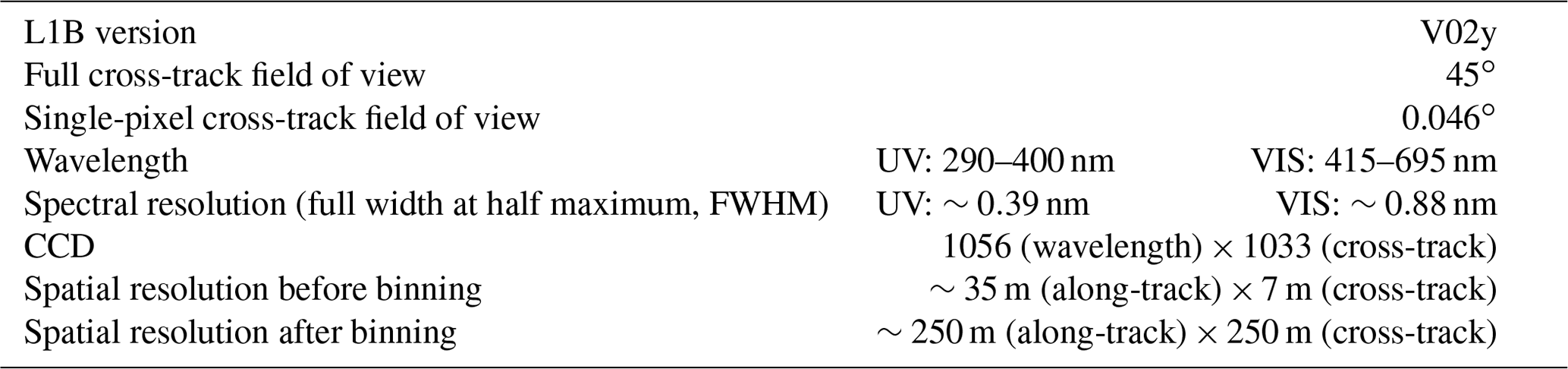
NO₂ VCDs were retrieved from the L1B radiance dataset (version: V02y) obtained using GeoTASO during the KORUS-AQ campaign. The NASA Goddard Space Flight Center conducted the L1B radiance calibration, which included offset and smear correction, gain matching, amplifier cross-talk correction, dark rate correction, integration normalization, sensitivity derivation, wavelength registration, geo-registration, nonlinearity correction, and ground pixel geolocation (Kowalewski et al., 2017; Chong et al., 2020). The detailed specifications of GeoTASO are listed in Table 2 (Nowlan et al., 2016).

Table 2 Summary of the GeoTASO instrument and optical specification.

Figure 2 Flowchart of the algorithm for retrieving tropospheric NO₂ data from GeoTASO.

2.4.1 NO₂ slant column density retrieval

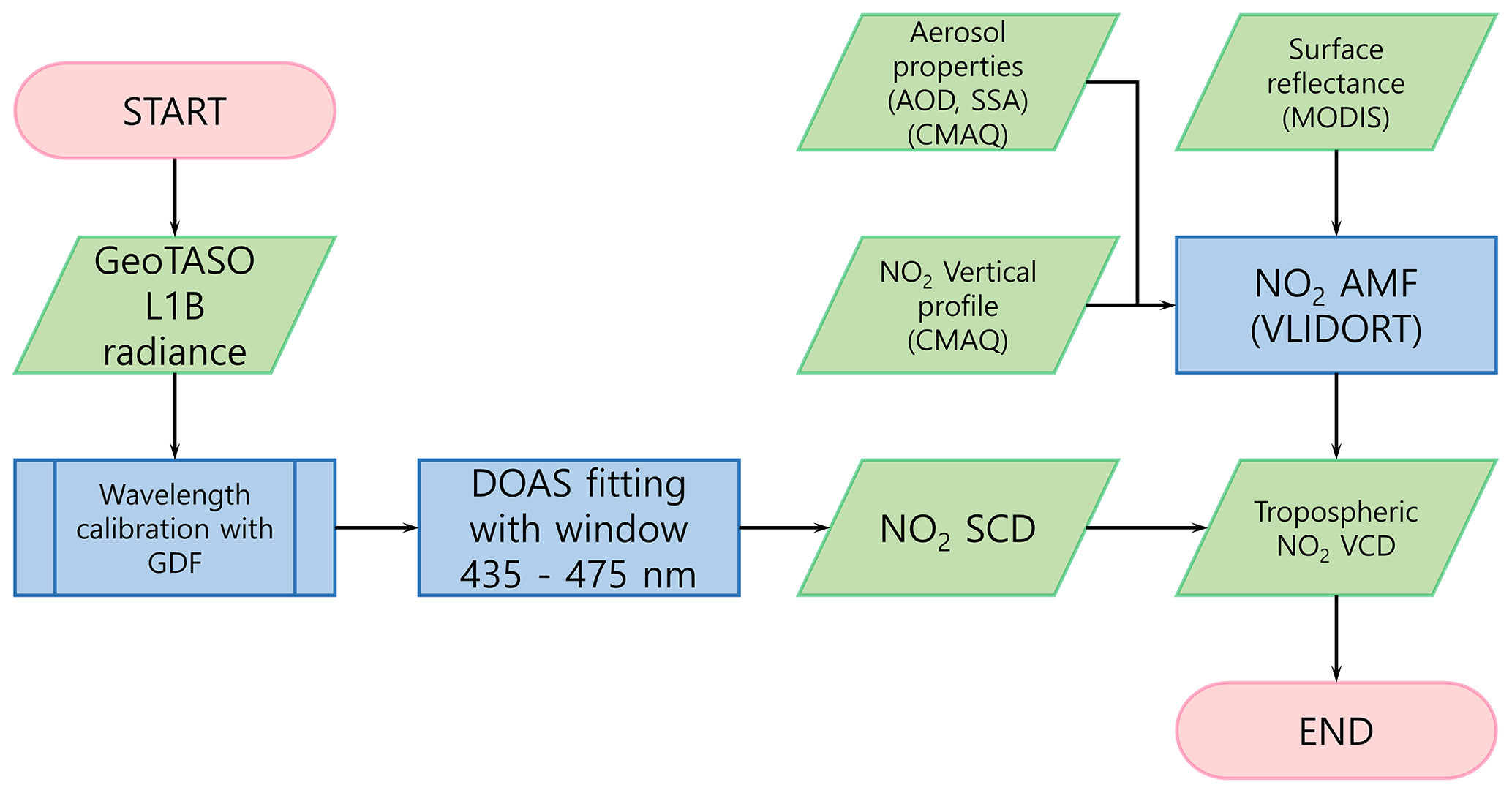
Figure 2 indicates the flowchart for retrieving the tropospheric NO₂ VCD from the GeoTASO. We first retrieved NO₂ SCDs using the DOAS method (Platt, 1994). Nonlinear least-squares minimization was used to retrieve the NO₂ SCDs, which minimizes the difference between the measured optical depth and the modeled value in QDOAS software (Eq. 1; Danckaert et al., 2012):

$$\begin{array}{}\text{(1)}& \begin{array}{rl}{\displaystyle \frac{\ln I\left(\mathit{\lambda }\right)}{\ln I_{\mathrm{0}}\left(\mathit{\lambda }\right)}}& =-\left(\sum _{j=\mathrm{1}}^m{\mathit{\rho }}_j\times {\mathit{\sigma }}_j^{\prime }\left(\mathit{\lambda }\right)+B\left(\mathit{\lambda }\right)\right.\\ & +R\left(\mathit{\lambda }\right)+A\left(\mathit{\lambda }\right)+N\left(\mathit{\lambda }\right)),\end{array}\end{array}$$

where I(λ) is the measured earthshine radiance at wavelength λ; I₀ is the reference radiance from the reference sector (ocean south of Jeju Island denoted with the red circle in Fig. 1; 32.983^∘ N, 126.392^∘ E) at 09:00 LT on 1 May 2016. The Community Multiscale Air Quality (CMAQ) modeling system data indicated that the NO₂ VCD from the surface to 50 hPa over this reference sector on this day was 6.75×10¹⁵ molec. cm⁻², and the mean of total NO₂ VCD obtained from the OMI during the KOURS-AQ period was 4.77×10¹⁵ molec. cm⁻² with a standard deviation of 1.33×10¹⁵ molec. cm⁻². We also confirmed the stability of NO₂ distribution over this area using the TROPOMI offline data from 2019 to 2020. In this period, the NO₂ VCD from the TROPOMI was 4.81×10¹⁵ molec. cm⁻² with a standard deviation of 0.43×10¹⁵ molec. cm⁻². The NO₂ VCD used as a reference sector obtained from CMAQ was mainly dominated by stratospheric NO₂ VCD. However, stratospheric NO₂ VCD has a relatively lower value compared to tropospheric NO₂ VCD. The ρ_j represents the SCD of each species j; ${\mathit{\sigma }}_j^{\prime }\left(\mathit{\lambda }\right)$ represents the differential gas phase absorption cross section convolved with the Gaussian distribution function (GDF) with GeoTASO FWHM (the UV and VIS range were 0.34–0.49 nm and 0.70–1.00 nm, respectively; Nowlan et al., 2016) at wavelength λ of species j, respectively.

We used the measured radiances at the reference sector to calculate differential slant column density (dSCD) over the whole domain of the GetoTASO measurements. CMAQ calculation over the reference sector (i.e., 6.75×10¹⁵ molec. cm⁻²) was adopted as the reference SCD (SC₀), which is added to all dSCD values to convert to the SCD. The reference sector is known as a background area but is occasionally affected by the long-range transport of NO₂ from upwind areas. Considering the standard deviation of the OMI measurements accounts for such effects during the measurement period, we estimate the maximum uncertainties of the SC₀ can be calculated from this value (i.e., 1.33×10¹⁵ molec. cm⁻²) in addition to the difference in the mean values between CMAQ and OMI (i.e., 1.98×10¹⁵ molec. cm⁻²). Therefore, our best estimate of the uncertainty of the SC₀ is the root of the sum of squares of these values (i.e., 2.38×10¹⁵ molec. cm⁻²).

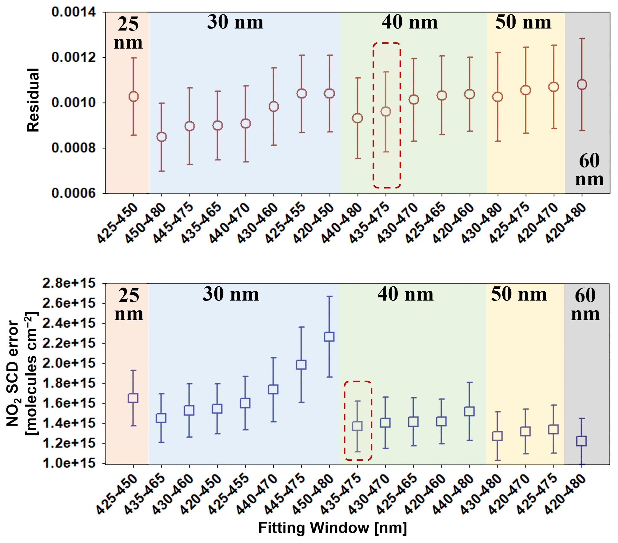
Figure 3 Residuals and NO₂ SCD errors of 17 spectral fitting window candidates (17 May 2016, with an across-track number of 15).

The spectral fitting window was selected based on the sensitivity test with 17 fitting window candidates from 420 to 480 nm with a fitting window length from 25 to 60 nm. Spectral fitting residuals and NO₂ SCD errors have been investigated for 17 spectral fitting window candidates (Fig. 3).

In terms of the residual, when the NO₂ fitting window includes a wavelength region less than 430 nm it has a larger residual compared to the case where it does not. The higher residual can include the more noise signals that cannot be calculated mathematically, which can become an uncertainty for the NO₂ SCD retrievals. Therefore, we excluded the fitting window, which includes wavelengths less than 430 nm for the GeoTASO NO₂ retrievals during the KORUS-AQ campaign. In the case of the NO₂ SCD error, it was confirmed that the longer the fitting window length was, the lower the NO₂ SCD error appeared regardless of including the wavelength region less than 430 nm. Therefore, for the stable NO₂ SCD retrieval, an appropriate spectral fitting window needs to be selected that can minimize the residual with a moderate length of the fitting window. To find the optimal fitting window, we set the threshold value based on the above results: residual <0.001, NO₂ SCD error $<\mathrm{1.4}\times {\mathrm{10}}^{\mathrm{15}}$ molec. cm⁻², and the length of fitting window >30 nm. Following this, the fitting window of 435–475 nm was selected for the GeoTASO NO₂ retrievals during the KORUS-AQ campaign. To determine the wavelength registration more accurately in the narrow fitting window, additional wavelength calibration of the spectra for each of the 33 across-track pixels was performed using a high-resolution solar reference spectrum (Kurucz solar spectrum) (Chance and Kurucz, 2010) with the GDF. The absorption cross sections of NO₂ (Vandaele et al., 1998), O₃ (Bogumil et al., 2000), H₂O (Rothman et al., 2010), and the Ring effect as pseudo-absorbers (Chance and Spurr, 1997) were used to construct the model equation, while B(λ), R(λ), A(λ), and N(λ) are the broad absorption of trace gases, extinction by Mie and Rayleigh scattering, variation in the spectral sensitivity of the detector or spectrograph, and noise, respectively, which were accounted for by an eighth-order polynomial. An example of the spectral fitting results is presented in Fig. 4.

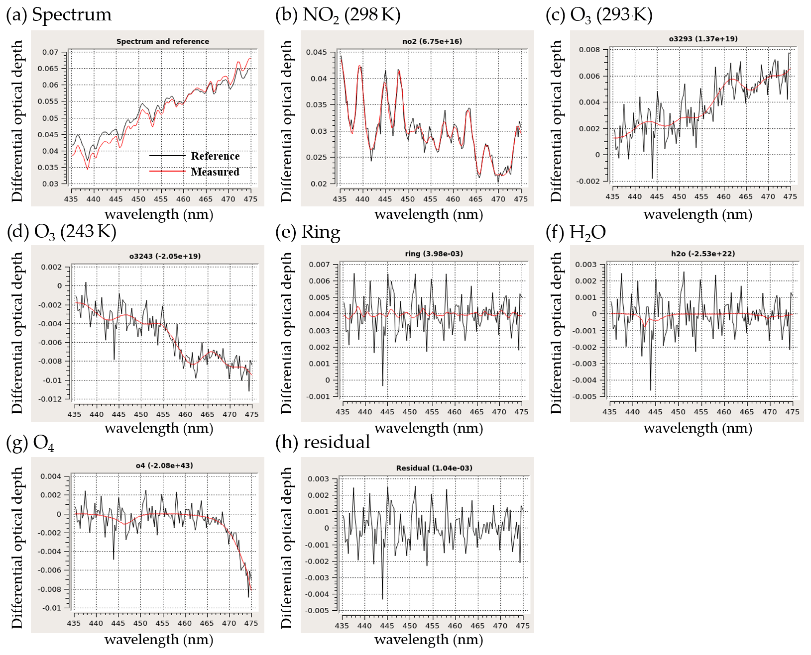
Figure 4 An example of the spectral fitting results of NO₂ retrievals from GeoTASO during the KORUS-AQ campaign (at Gangnam, Seoul on 9 June 2016). The red and black line in panel (a) represent the measured and reference spectrum, respectively. Panels (b) to (h) depict examples of spectral fitting results of (b) NO₂, (c) O₃ (293 K), (d) O₃ (243 K), (e) Ring effect, (f) H₂O, and (g) O₄, where red and black lines are the absorption cross section of the target species and the fitting residual plus the absorption of the target species, respectively. Panel (h) indicates the fitting residual of this example.

2.4.2 NO₂ AMF calculation

AMF, the ratio of SCD to VCD, can be calculated using the scattering weight (ω) and shape factor (S) (Palmer et al., 2001) in Eq. (2)–(5):

$$\begin{array}{}\text{(2)}& {\displaystyle }\mathrm{AMF}={\displaystyle \frac{\mathrm{SCD}}{\mathrm{VCD}}},\text{(3)}& {\displaystyle }\mathrm{AMF}={\mathrm{AMF}}_{\mathrm{G}}\underset{z\mathrm{1}}{\overset{z\mathrm{2}}{\int }}\mathit{\omega }\left(z\right)S\left(z\right)\mathrm{d}z,\end{array}$$

$$\begin{array}{}\text{(4)}& {\displaystyle }\mathit{\omega }\left(z\right)=-{\displaystyle \frac{\mathrm{1}}{{\mathrm{AMF}}_{\mathrm{G}}}}{\displaystyle \frac{\partial \ln I_{\mathrm{B}}}{\partial \mathit{\tau }}},\text{(5)}& {\displaystyle }S\left(z\right)={\displaystyle \frac{\mathit{\alpha }\left(z\right)n\left(z\right)}{{\int }_{z\mathrm{1}}^{z\mathrm{2}}\mathit{\alpha }\left(z\right)n\left(z\right)\mathrm{d}z}},\end{array}$$

where AMF_G represents the geometric AMF, I_B is the earthshine radiance, τ is the optical depth, α is the absorption cross section, and n is the number density of the absorber. NO₂ AMF was calculated using a linearized pseudo-spherical scalar and vector discrete ordinate radiative transfer model (VLIDORT, version 2.6; Spurr and Christi, 2014). Aerosol properties, such as AOD, SSA, APH, and a priori NO₂ vertical profile information, were simulated using the CMAQ, and surface reflectivity was obtained from MODIS (Collection 6). The SR products, MCD43A3, available at a 500 m spatial resolution, provide an estimate of the surface spectral reflectance including MODIS bands 1 through 7. Here, MODIS band 3 (459–479 nm) was used because this band is the closest the wavelength (455 nm) used in the calculation of AMF in this study. APH was assumed to be the peak height of the aerosol extinction coefficient simulated in CMAQ, and the aerosol profile applied GDF based on APH (Hong et al., 2017). For pixels without reflectance information, AMF was not calculated. The products were corrected for atmospheric conditions, such as aerosol, gases, and Rayleigh scattering. In previous studies (Lamsal et al., 2017; Nowlan et al., 2018; Judd et al., 2019; Chong et al., 2020), an AMF was described for both above and below aircraft altitude is used to convert NO₂ SCDs to VCDs using Eqs. (6)–(8).

$$\begin{array}{}\text{(6)}& {\displaystyle }\mathrm{AMF}\uparrow ={\mathrm{AMF}}_{\mathrm{G}}\underset{Z_{\mathrm{A}}}{\overset{Z_{\mathrm{TOA}}}{\int }}\mathit{\omega }\left(z\right)S\left(z\right)\mathrm{d}z,\text{(7)}& {\displaystyle }\mathrm{AMF}\downarrow ={\mathrm{AMF}}_{\mathrm{G}}\underset{Z_{\mathrm{0}}}{\overset{Z_{\mathrm{A}}}{\int }}\mathit{\omega }\left(z\right)S\left(z\right)\mathrm{d}z,\text{(8)}& {\displaystyle }{\mathrm{NO}}_{\mathrm{2}}\mathrm{VCD}\downarrow ={\displaystyle \frac{{\mathrm{NO}}_{\mathrm{2}}\mathrm{SCD}-\mathrm{AMF}\uparrow \cdot {\mathrm{NO}}_{\mathrm{2}}\mathrm{VCD}\uparrow }{\mathrm{AMF}\downarrow }},\end{array}$$

where AMF↑ and AMF↓ are AMF above and below aircraft, respectively, and NO₂ VCD↑ represents NO₂ VCD above the aircraft obtained from a chemical transport model (CTM). However, here we calculated the NO₂ VCD↓ by dividing NO₂ SCDs by AMF↓ as the CMAQ only simulates the troposphere (surface to 50 hPa). However, as the stratospheric and free tropospheric NO₂ (NO₂ VCD↑) column densities over megacities and industrial areas are much lower than tropospheric NO₂ column densities (Valks et al., 2011), we assume that the uncertainties in the AMF without considering the upper atmosphere are negligible in this study.

2.5 Chemical model description

Vertical profiles from CMAQ (Byun and Ching, 1999; Byun and Schere, 2006), a CTM, were used to calculate AMFs. The CMAQ simulations were conducted with a horizontal resolution of 15×15 km and had 27 vertical layers from the surface to 50 hPa. The meteorological fields were prepared using the advanced research Weather Research and Forecasting (WRF) Advanced Research WRF (ARW) Model (Skamarock et al., 2008). Anthropogenic emissions were generated based on the KORUS v5.0 model (Woo et al., 2012), and biogenic emissions were simulated using the Model of Emissions of Gases and Aerosols from Nature (MEGAN v2.1; Guenther et al., 2006, 2012). Besides anthropogenic and biogenic emissions, the Fire Inventory from NCAR (FINN; Wiedinmyer et al., 2006, 2011) was used to update the pyrogenic emission fields.

The CMAQ AOD was calculated by integrating the aerosol extinction coefficient (Q_ext), which is the sum of scattering (Q_sca) and absorption (Q_abs) coefficients over all vertical layers (z) as follows:

$$\begin{array}{}\text{(9)}& {\displaystyle }\mathrm{AOD}=\int Q_{\mathrm{ext}}\left(z\right)\mathrm{d}z=\int \left\{Q_{\mathrm{sca}}\left(z\right)+Q_{\mathrm{abs}}\left(z\right)\right\}\mathrm{d}z,\text{(10)}& {\displaystyle }{Q}_{\mathrm{abs}}\left[{\mathrm{Mm}}^{-\mathrm{1}}\right]=\sum _i\sum _j\left\{(\mathrm{1}-{\mathit{\omega }}_{ij})\cdot {\mathit{\beta }}_{ij}\cdot f_{ij}\left(\mathrm{RH}\right)\cdot [C{]}_{ij}\right\},\text{(11)}& {\displaystyle }{Q}_{\mathrm{sca}}\left[{\mathrm{Mm}}^{-\mathrm{1}}\right]=\sum _i\sum _j\left\{{\mathit{\omega }}_{ij}\cdot {\mathit{\beta }}_{ij}\cdot f_{ij}\left(\mathrm{RH}\right)\cdot [C{]}_{ij}\right\},\end{array}$$

where ω_ij indicates SSA of particulate species i for the particulate mode (or size bin) j, β_ij denotes the mass extinction efficiency, f_ij(RH) is the hygroscopicity factor according to the relative humidity (RH), and [C]_ij is the concentration of particulate species. CMAQ SSA is defined as the ratio of the integrated Q_sca to AOD, and NO₂ vertical profiles were obtained from NO₂ concentrations at each vertical layer by conducting CMAQ simulations. Details of the model descriptions and calculations of optical properties are given by Lee et al. (2020) and Malm and Hand (2007).

3 Results and discussion

3.1 NO₂ VCD retrieval

3.1.1 Seoul metropolitan region

We show the final NO₂ VCDs from 250 m spatial resolution. Because of NO₂ VCD, we selected the dates observed in both the morning and afternoon during the KORUS-AQ period over the Seoul metropolitan area, Busan, and Anmyeon. The retrieved dates for NO₂ VCDs were 5, 9, and 10 June 2016.

The population of the Seoul metropolitan region is approximately 20 million, which is approximately 40 % of the total population of South Korea. It is rare to obtain high-resolution horizontal NO₂ VCD distributions using airborne measurements in the morning and afternoon, especially in Asian megacities. Figure 5 indicates tropospheric NO₂ VCDs over Seoul on 9 June 2016, at 09:00 and 15:00 LT. Because of an issue with the imaging systems, enlarged views (Figs. 5–8) present a slightly stripy appearance from the GeoTASO observation (Nowlan et al., 2016; Chong et al., 2020).

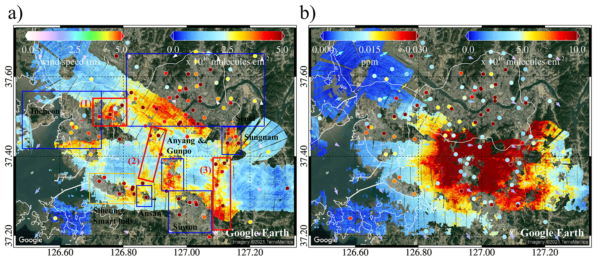
Figure 5 Tropospheric NO₂ VCD in the Seoul metropolitan region on 9 June 2016 retrieved from GeoTASO (a) at 09:00 and (b) at 15:00 LT. The red boxes represent expressways (counterclockwise from left to right, (1) Gyeongin Expressway, (2) Seohaean Expressway, and (3) Gyeongbu Expressway), the orange box indicates the industrial complex, and the blue boxes indicate the major cities (Seoul, Incheon, Suwon, Bucheon, Anyang, Gunpo, Sungnam, and Ansan) of the Seoul metropolitan region. The colors of the circles depict the NO₂ surface mixing ratio obtained from Air-Korea. The colored arrows indicate the wind direction and speed at 1000 hPa over the Seoul metropolitan region obtained via the Unified Model (UM) simulations (the background RGB image is from Google Earth; https://www.google.com/maps/, last access: 19 January 2023).

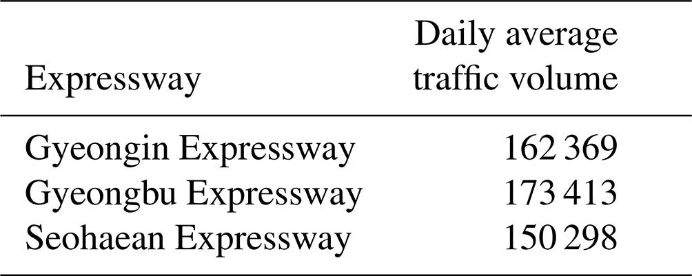
In the morning, NO₂ VCDs retrieved from GeoTASO were highly correlated with expressways (red boxes in Fig. 5), such as the Gyeongin, Seohaean, and Gyeongbu expressways, and over major cities with heavy traffic, such as Seoul, Bucheon, Ansan, Anyang, and Suwon. GeoTASO observed NO₂ VCD values that were 3 times higher ($>\mathrm{3}\times {\mathrm{10}}^{\mathrm{16}}$ molec. cm⁻²) in these areas compared to the surrounding rural areas. High NO₂ VCD values above 6×10¹⁶ molec. cm⁻² were observed above the Gyeongin Expressway, which has very heavy traffic in a relatively short section, and the Gunpo Complex Logistics zone, where diesel vehicle traffic is also high. The main NO₂ source regions and the regions where high NO₂ VCD values were observed were highly consistent at 09:00 LT because the wind speed at this time – as obtained from the Unified Model (UM)-based Regional Data Assimilation and Prediction System (RDAPS) of the Korea Meteorological Administration (KMA) – was as low as 0.1 ms⁻¹, and the average wind direction was 84.7^∘ at 1000 hPa over Seoul metropolitan region. The average daily traffic volume of these expressways exceeds 150 000 vehicles, and the total number of vehicles registered in these major cities is >6 000 000, with an average daily mileage per car per day of over 38 km. Detailed information on these cities and expressways is listed in Tables 3 and 4. Based on the level of vehicular traffic, combustion using gasoline and diesel engines leads to high overall emissions of NO₂ in the Seoul metropolitan region (Kendrick et al., 2015).

Table 3 The population, number of registered vehicles, and average mileage per car per day of the major cities in the Seoul and Busan metropolitan region obtained from the Korean Statistical Information Service (https://kosis.kr/eng, last access: 25 March 2022).

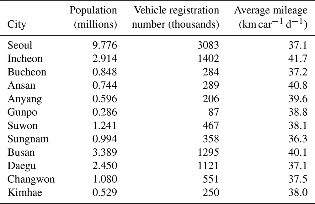
Table 4 Daily average traffic volume on the Gyeongin, Gyeongbu, and Seohaean expressways obtained using the Traffic Monitoring System (https://www.road.re.kr, last access: 28 February 2022).

Compared to the data of the morning, the average wind speed and wind direction were 1.7 ms⁻¹ and 284.5^∘ at 1000 hPa in the afternoon, and the afternoon had extremely high tropospheric NO₂ VCD values (exceeding 5×10¹⁶ molec. cm⁻²) in most of the Seoul metropolitan region, including rural areas, whereas the NO₂ mixing ratio (MR) obtained from Air-Korea decreases in the afternoon. According to Tzortziou et al. (2018), similar results were retrieved from the Pandora site in Seoul, with higher afternoon NO₂ VCDs than in the morning. This result is because the amount of NO₂ produced by chemical conversion of nitric oxide (NO) by O₃ and VOCs in the atmosphere, along with NO_x generated by regional emissions (traffic) in the Seoul metropolitan region, is greater than the amount lost by photolysis and transport to nearby areas (Herman et al., 2018). Furthermore, the increase in tropospheric NO₂ VCD in the afternoon is likely due to the accumulation and dispersion of NO₂ according to the height of the change in the planetary boundary layer (Ma et al., 2013).

3.1.2 Industrial and power plant regions in Anmyeon

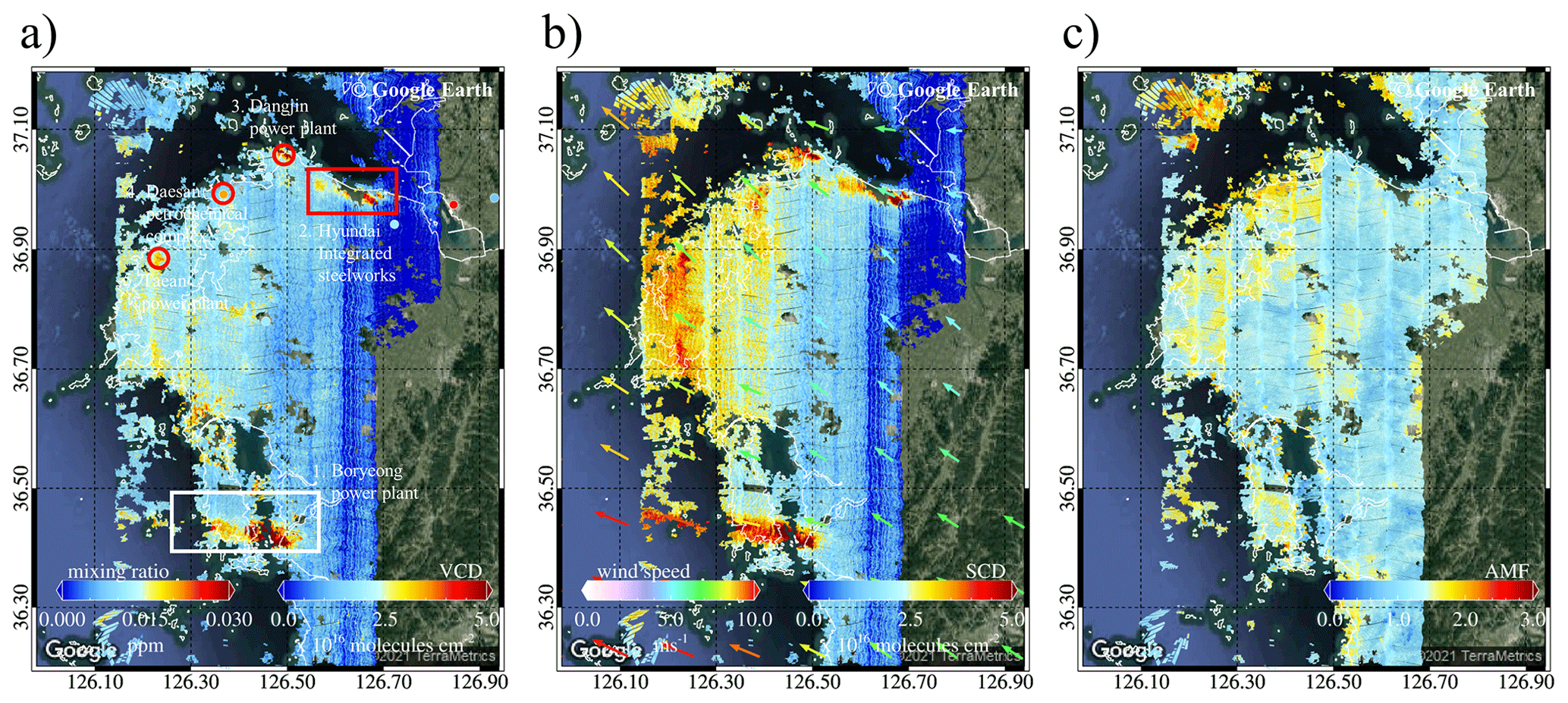
Figure 6 (a) Tropospheric NO₂ VCD and (b) NO₂ SCD retrieved from GeoTASO and (c) NO₂ AMF at native resolution (250 m) calculated using VLIDORT over Anmyeon in South Korea on 5 June 2016. The colored arrows indicate wind speed and wind direction at 850 hPa from the Unified Model (UM) simulations. The red circles and rectangle in (a) represent the major NO₂ emission sources, such as steelworks and power plants (background RGB image is from Google Earth; https://www.google.com/maps/, last access: 19 January 2023).

The high spatial resolution of the tropospheric NO₂ VCD from GeoTASO over the Anmyeon industrial region, where many industrial facilities and several power plants are distributed, is shown in Fig. 6. Figure 6a and b indicate tropospheric NO₂ VCD and NO₂ SCD retrieved from GeoTASO L1B data, respectively, between 13:00 and 17:00 LT on 5 June 2016. Figure 6c depicts the calculated AMF of NO₂ from native resolution over the domain. GeoTASO observations detected the following moderate and strong NO₂ emission sources in this area: (1) Boryeong power plant, (2) Hyundai integrated steelworks, (3) Dangjin power plant, (4) Daesan petrochemical complex, and (5) Taean power plant. High NO₂ VCD values ($>\mathrm{5}\times {\mathrm{10}}^{\mathrm{16}}$ molec. cm⁻²) were observed over steel mill works, petrochemical complexes, and power plants, whereas values were comparatively low ($<\mathrm{1}\times {\mathrm{10}}^{\mathrm{16}}$ molec. cm⁻²) over small cities with populations of less than 0.1 million, including Seosan, Dangjin, and Boryeong, and the Seohaean Expressway. In 2016, the annual NO_x emissions from the Hyundai steelworks and the Dangjin and Boryeong power plants were approximately 10.3, 11.9, and 16.8 kt yr⁻¹, respectively. The NO_x emission rates of major industrial facilities in the Anmyeon region are shown in Table 5.

Table 5 NO_x emission rates in 2016 from major industrial facilities in the Anmyeon region obtained from the Continuous Emission Monitoring System of the Korea Environment Corporation (https://www.stacknsky.or.kr/eng/index.html, last access: 25 March 2022).

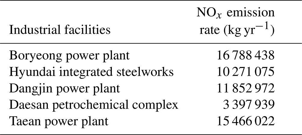
Figure 6 shows high NO₂ concentrations of the main industrial facilities in the Anmyeon region, where the combustion of fossil fuel in factories and thermal power plants leads to high emissions (Prasad et al., 2012). Due to relatively sparse distribution over rural areas, the Air-Korea measurements did not detect the major NO₂ plume as shown in Fig. 6a. Thus, airborne remote sensing systems, such as GeoTASO, can effectively complement ground-based networks for monitoring minor and major NO_x emissions, particularly over these remote industrial regions.

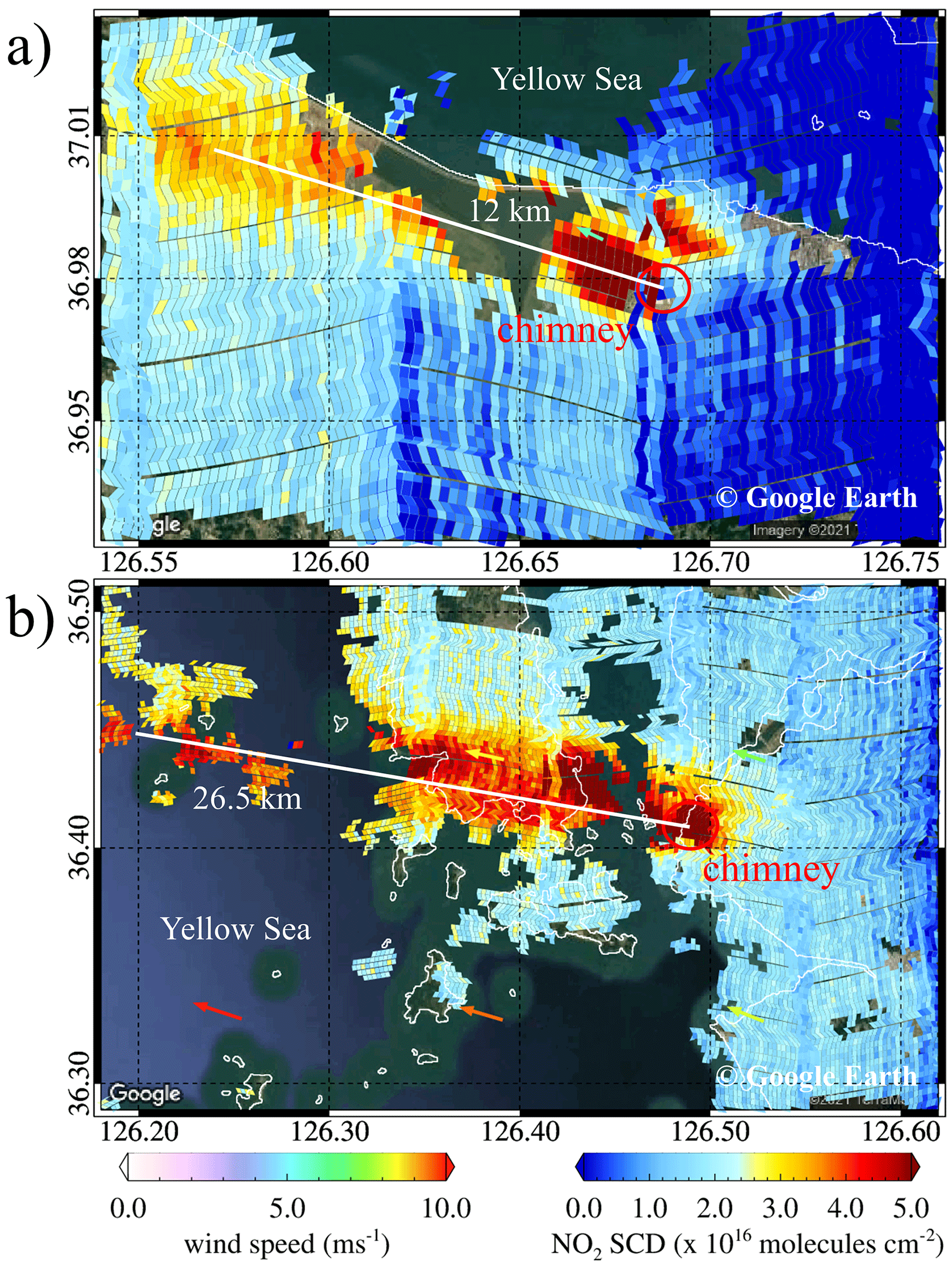
Figure 7 Enlarged view of GeoTASO tropospheric NO₂ SCD observation over (a) the Hyundai steel works, indicated by the red box in Fig. 6, and (b) the Boryeong power plant, indicated by the white box in Fig. 6. The arrows represent the wind direction and speed at 850 hPa from the Unified Model (UM) simulations (the background RGB image is from Google Earth; https://www.google.com/maps/, last access: 19 January 2023).

The GeoTASO data captured not only NO_x emissions from the chimneys of steelworks and power plants but also its transport by the wind. Figure 7a and b show enlarged views of tropospheric NO₂ SCD retrieved using GeoTASO over the Hyundai steelworks (red box in Fig. 6) and the Boryeong power plant (white box in Fig. 6). The arrows in Fig. 7 represent the prevailing wind direction and speed from RDAPS. NO₂ emitted from the chimneys of these sites was transported to the Yellow Sea, traveling distances of over 26.5 km at speeds of approximately 6 ms⁻¹. According to Chong et al. (2020), similar results were found for SO₂ emitted and transported from these sites.

3.1.3 Busan metropolitan region

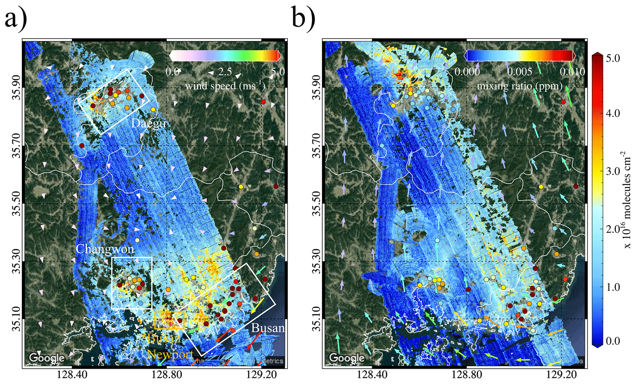
Figure 8 Tropospheric NO₂ VCD in the Busan metropolitan region in the (a) morning and (b) afternoon of 10 June 2016. The wind speed (color scale) and wind direction (arrows) at 1000 hPa pressure level were obtained from the Unified Model (UM) simulations. The white boxes represent the major cities of Busan, Daegu, and Changwon. The orange box represents Busan New Port (the background RGB image is from Google Earth; https://www.google.com/maps/, last access: 19 January 2023).

Figure 8a and  b show tropospheric NO₂ VCD retrieved from the GeoTASO L1B data over the Busan metropolitan region on 10 June 2016 in the morning (between 08:00 and 11:00 LT) and afternoon (between 13:00 and 16:00 LT), respectively. The arrows in Fig. 8 indicate the wind speed and wind direction at 1000 hPa obtained from the UM-RDAPS, with the average wind speed and wind direction of 0.9 ms⁻¹ and 55.4^∘ and 1.9 ms⁻¹ and 147.0^∘, respectively, in the morning and afternoon. High NO₂ VCDs were observed above urban areas, ports, industrial complexes, and the inter-city road between Busan and Changwon. Like the Seoul metropolitan region, combustion using gasoline and diesel engines is estimated to contribute to the high NO_x emission. In the morning, NO₂ VCDs were high (approximately 3×10¹⁶ molec. cm⁻²) in the major cities and especially around Busan New Port, with values exceeding 7×10¹⁶ molec. cm⁻². In comparison, in the mountainous regions between Daegu and Busan, the NO₂ VCD values were less than 1×10¹⁶ molec. cm⁻² during the same period. The spatial distribution of tropospheric NO₂ VCDs was similar in the Seoul metropolitan regions, with high values over major cities and roads (compare Figs. 5 and 8). In Busan, fossil fuel combustion in use by both road vehicles and ships is likely to contribute to the NO_x emissions. In the afternoon, unlike the Seoul metropolitan region, tropospheric NO₂ VCD over Busan decreased by over 3×10¹⁶ molec. cm⁻², which also corresponds with NO₂ MR data obtained from the Air-Korea sites. Detailed information on these cities is listed in Table 3.

3.2 Error estimation

The accuracy of the NO₂ VCD retrieval using the DOAS method depends on both the AMF calculation and the spectral fitting error of the SCD retrieval. Retrieval errors of the NO₂ VCD were estimated using error propagation analysis as expressed in Eq. (12):

$$\begin{array}{}\text{(12)}& {\displaystyle \frac{{\mathit{\epsilon }}_{\mathrm{VCD}}}{\mathrm{VCD}}}=\sqrt{({\displaystyle \frac{{\mathit{\epsilon }}_{\mathrm{SCD}}}{\mathrm{SCD}}}{)}^{\mathrm{2}}+({\displaystyle \frac{{\mathit{\epsilon }}_{\mathrm{AMF}}}{\mathrm{AMF}}}{)}^{\mathrm{2}}},\end{array}$$

where ε_VCD is the total error of NO₂ VCD. The error of NO₂ SCD (ε_SCD) is obtained from the spectral fitting error of NO₂ SCD via the DOAS spectral fitting. ε_AMF indicates the error of NO₂ AMF caused by uncertainties in the model input parameters for AMF calculation. Uncertainties in aerosol properties (AOD, SSA, and APH) and SR for the radiative transfer model (RTM) calculations are the major factors affecting NO₂ AMF accuracy (Boersma et al., 2004; Leitão et al., 2010; Hong et al., 2017). Therefore, in this present study we quantified the NO₂ AMF errors (ε_AMF) due to uncertainties in the input parameters independent of each other using Eq. (13):

$$\begin{array}{}\text{(13)}& \begin{array}{rl}{\mathit{\epsilon }}_{\mathrm{AMF}}& =\sqrt{{\left({\displaystyle \frac{\partial \mathrm{AMF}}{\partial \mathrm{AOD}}}\right)}^{\mathrm{2}}\mathit{\sigma }{\mathrm{AOD}}^{\mathrm{2}}+{\left({\displaystyle \frac{\partial \mathrm{AMF}}{\partial \mathrm{SSA}}}\right)}^{\mathrm{2}}\mathit{\sigma }{\mathrm{SSA}}^{\mathrm{2}}}\\ & +\stackrel{\mathrm{‾}}{{\left({\displaystyle \frac{\partial \mathrm{AMF}}{\partial \mathrm{ALH}}}\right)}^{\mathrm{2}}\mathit{\sigma }{\mathrm{ALH}}^{\mathrm{2}}+{\left({\displaystyle \frac{\partial \mathrm{AMF}}{\partial \mathrm{SR}}}\right)}^{\mathrm{2}}\mathit{\sigma }{\mathrm{SR}}^{\mathrm{2}}}\\ & =\sqrt{\sum _{i=\mathrm{1}}^{\mathrm{4}}{\left({\displaystyle \frac{\partial \mathrm{AMF}}{\partial {\mathit{\chi }}_i}}\right)}^{\mathrm{2}}{\mathit{\sigma }}_{{\mathit{\chi }}_i}^{\mathrm{2}}},\end{array}\end{array}$$

where $\frac{\partial \mathrm{AMF}}{\partial {\mathit{\chi }}_i}$ are partial derivatives of NO₂ AMF regarding the input parameters (χ_i), σ_χi represents the uncertainty of the χ_i. The σ of AOD, SSA, SR, and APH are assumed to be 30 % (Ahn et al., 2014), 0.04 (Jethva et al., 2014), 0.005 + 0.05 × SR (EOS Land Validation; https://landval.gsfc.nasa.gov, last access: 22 July 2022), and 1 km (Fishman et al., 2012), respectively, in this study. To derive $(\frac{\partial \mathrm{AMF}}{\partial {\mathit{\chi }}_i}{)}^{\mathrm{2}}$, the true χ_i is input to the RTM to simulate “true” NO₂ AMF. For the AOD, SSA, APH, and SR, perturbed NO₂ AMF was simulated using RTM with χ_i±σχ_i. ∂χ_i denotes the difference between the “center” χ_i and χ_i±σχ_i, and ∂AMF is the difference between the “center” NO₂ AMF (AMF_centre) simulated with “center” input values and the perturbed NO₂ AMF (AMF_perturbed) simulated using the perturbed input parameters χ_i±σχ_i (i.e., the original input parameters modified by the uncertainty). The simulation for calculating the ε_AMF was conducted using the input parameters on 9 June 2016.

Table 6 Total NO₂ VCD caused by uncertainties in NO₂ SCD and NO₂ AMF (the average for the flight on 9 June 2016).

Table 6 lists the estimated NO₂ VCD error on 9 June 2016 for each source based on the error propagation method. The error estimation was conducted for the pixels where the root-mean-square residual is <0.001 and NO₂ VCD > 5 × 10¹⁵ molec. cm⁻² since NO₂ SCD precision is reported to be highly decreased in low NO₂ conditions (Hong et al., 2017). The total NO₂ VCD error was 26.9 %, with a high portion of NO₂ AMF error. The NO₂ SCD error was calculated to be 11.7 %, showing the importance of accurate DOAS spectral fitting for deriving NO₂ SCD. The total AMF error due to uncertainties in the input parameters was calculated to be 23.3 %. Among model input parameters, the effect of APH on NO₂ AMF becomes high (22.3 %), indicating the importance of accurate aerosol profile information. APH sensitivity affects NO₂ AMF because aerosols lead to multiple scattering effects near the surface where trace gases and aerosols are well mixed, and the light absorption of trace gases is due to the increasing light path (Castellanos et al., 2015; Hong et al., 2017). APH has the potential to be the most important input parameter in the Asia region where high loadings of aerosol plumes persist throughout the year. The NO₂ AMF calculation errors due to uncertainties in SSA and AOD were 4.1 % and 2.8 %, respectively. The NO₂ AMF calculation error due to uncertainties in aerosol optical properties (SSA and AOD) appears to be smaller than those in a previous study (Leitão et al., 2010). The smaller effect of the aerosol properties can be explained by the moderate aerosol loading (AOD = 0.40) on the day of flight day. The NO₂ AMF errors become larger under high AOD conditions. The smallest effect of SR was found on NO₂ AMF calculation error, which was calculated based on the uncertainty of the SR of the satellite-based product (MODIS). Therefore, it may be an unrealistic number for the airborne NO₂ AMF calculation. Once the uncertainty of airborne-based SR is provided, considering its measurement geometry and finer spatial resolution, more realistic airborne-based NO₂ AMF calculation error due to uncertainties in SR can be estimated. The a priori NO₂ profile shape can also be a factor that causes a calculation error for the NO₂ AMF, as reported in previous studies (Leitão et al., 2010, Meier et al., 2017; Hong et al., 2017). Therefore, it is necessary to calculate the contribution of the shape of the a priori NO₂ profile to the accuracy of NO₂ AMF in the future. Moreover, the resulting uncertainties in input parameters of a GeoTASO ground pixel need to be considered by combining the initial uncertainties of CTM and satellite-based products and by using the variability of the parameters within the respective CTM (AOD, SSA, and APH) and satellite (SR) grid box. If values such as SR are assumed constant over larger areas, the fundamental spatial variability in these data increases the uncertainty of the AMF and hence of the determined NO₂ VCD on the respective finer spatial scale. In addition, the uncertainty from the assumption on the SC₀ and the uncertainty from ignoring the NO₂ above the aircraft in the AMF calculations both need to be considered in the error analysis. This analysis should be considered in a further study.

$$\begin{array}{}\text{(14)}& {\mathrm{AMF}}_{\mathrm{percent}\mathrm{\_}\mathrm{change}}={\displaystyle \frac{{\mathrm{AMF}}_{\mathrm{perturbed}}-{\mathrm{AMF}}_{\mathrm{center}}}{{\mathrm{AMF}}_{\mathrm{center}}}}\times \mathrm{100}.\end{array}$$

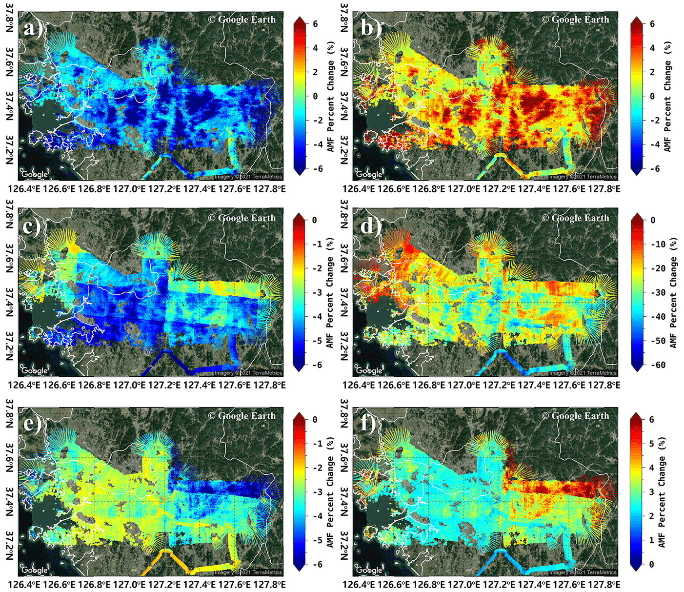
Figure 9 Percent change between AMF calculated using the CMAQ model simulation and those using (a) 30 % lower AOD, (b) 30 % higher AOD, (c) 0.04 lower SSA, and (d) 1 km higher APH compared to the model outputs. The percentage change for AMF calculated using MODIS data and those using (e) $\mathrm{0.005}+\mathrm{0.05}\times$ SR lower SR and (f) 0.005 + 0.05 × SR higher SR are also shown (the background RGB image is from Google Earth; https://www.google.com/maps/, last access: 19 January 2023).

In this study, we also investigated the spatial distribution of AMF calculation errors associated with uncertainties in aerosol properties (AOD, SSA, and APH) and SR. The percent change in NO₂ AMF (AMF_{percent_change}) was calculated on each spatial pixel using Eq. (14). Figure 9a and b indicate the percentage change error between the calculated AMFs using the CMAQ AOD data with 30 % lower (Fig. 9a) and 30 % higher (Fig. 9b) values, respectively. The AMF decreased and increased by up to 10 % with decreasing and increasing AOD, respectively, in the Seoul metropolitan region. We estimated that, under low aerosol loading conditions, an increase in AOD near the surface leads to an increase in the scattering probability within the surface layer with high NO₂ concentrations. Figure 9c indicates the percent change error between the calculated AMFs using CMAQ SSA data with a 0.04 lower value. The AMF decreased with decreasing SSA because the absorption of light increased. APH was also found to greatly affect the accuracy of the AMF calculations (Fig. 9d). The APH uncertainty of 1 km decreased the AMFs with an average AMF_{percent_change} of −25 % on the flight day. On the pixels where AOD > 0.6 in particular, the average AMF_{percent_change} was found to be −26 %, whereas this value was −27 % on the pixels where AOD > 0.4, showing the combined effect of aerosol loading and aerosol profile shape on the NO₂ AMF calculations. Figure 9e and f indicate the percentage change error between the calculated AMFs using the MODIS SR data with 0.005 + 0.05 × SR lower (Fig. 9e) and 0.005 + 0.05 × SR higher (Fig. 9f) values, respectively. The AMF decreased by approximately 3 % when the SR decreases, with the opposite occurring when it increased.

3.3 Validation of NO₂ VCDs retrieved from GeoTASO

The tropospheric NO₂ VCDs retrieved from GeoTASO L1B data (NO_2,G) were compared with those obtained from OMI total NO₂ VCDs (NO_2,O) and Pandora (NO_2,P). The NO_2,O were only available for 10 June during the campaign period. Therefore, we compared only 48 NO_2,G and NO_2,O data points within a radius of 20 km and 30 min, which yielded a correlation coefficient of 0.48 with a slope of 0.13 (Fig. 10a). To validate this data, all NO_2,G within a radius 20 km of the OMI center coordinate were averaged.

The NO₂ values are relatively low, as GeoTASO observation is conducted in a region with low NO₂ compared to the Seoul metropolitan region, and the overpass time of OMI is approximately 13:30 LT when NO₂ decreased. The low slope value is because the OMI with low spatial resolution does not reflect the spatial NO₂ inhomogeneity in the pixel.

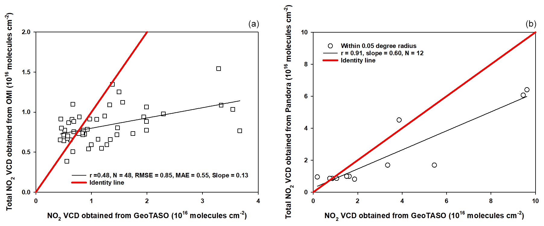
Figure 10 Scatter plots of (a) NO₂ VCD retrieved from GeoTASO and total NO₂ VCD obtained from OMI and (b) total NO₂ VCD obtained from Pandora and NO₂ VCD retrieved from GeoTASO, respectively.

To compare NO_2,G data, we made a comparison with total NO₂ VCD obtained from the Pandora system (NO_2,P) during the KORUS-AQ campaign period. NO_2,P obtained from Busan University, Olympic Park, Songchon, Yeoju, and Yonsei University Pandora sites on 5, 9, and 10 June were used for the GeoTASO validation (Fig. 1). NO_2,G and NO_2,P columns at these sites are compared in Fig. 11. To compare NO_2,G and NO_2,P, we used averaged NO_2,G retrieved from 16 across-track runs with the smallest viewing zenith angle possible and averaged 30 min NO₂ data obtained from Pandora measurements within a radius of approximately 0.05^∘. NO_2,G and NO_2,P were correlated (R=0.91, with a slope of 0.60); however, when NO_2,P was lower than 1×10¹⁶ molec. cm⁻², the correlation coefficient between NO_2,G and NO_2,P was <0.1. The weak correlation at low NO₂ levels most likely reflects differences in viewing geometries and the horizontal inhomogeneity of the measured NO₂ between Pandora and GeoTASO. Furthermore, Pandora and GeoTASO can be used for the NO₂ validation of geostationary satellites, such as GEMS. However, because the number of Pandora measurements is limited in this campaign, we have difficulty validating NO₂ retrieved from GeoTASO under various conditions. Many ground-based remote sensing measurements are needed to validate GEMS under various conditions.

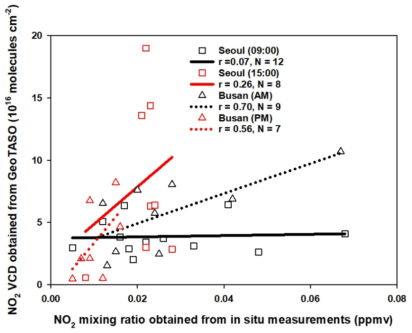
Figure 11 Scatter plot of the NO₂ VCDs retrieved from GeoTASO and the NO₂ surface mixing ratio obtained from Air-Korea. The black and red squares represent the NO₂ data at 09:00 and 15:00 LT in the Seoul metropolitan region, respectively. The black and red triangles represent those in the morning and afternoon over Busan, respectively.

To compare the spatiotemporal distribution of NO₂ VCDs retrieved from GeoTASO, NO_2,G was compared with surface spatial patterns and NO_2,G was compared with NO_2,A for GeoTASO data within a radius of approximately 0.05 km and 30 min (Fig. 11). To compare NO_2,G and NO_2,A, we used averaged NO_2,G retrieved from 16 across-track runs and averaged 30 min within a radius of 0.05^∘. Because in situ measurements provide NO₂ volume mixing ratio (VMR) (NO_2,A) (ppmv) once per hour, NO_2,A of the nearest time is used to compare with NO_2,G. The correlation coefficient (R) between NO_2,G (molec. cm⁻²) and NO_2,A at 09:00 and 15:00 LT in the Seoul metropolitan region was 0.07 and 0.26, respectively. When using only roadside station data from Air-Korea, the R value for the morning increased to 0.72, which implies GeoTASO is more sensitive to emissions from NO₂ source areas, such as roadsides (Fig. 5). During the comparison there were large differences in the morning and afternoon. These results were identified because synoptic meteorology played an important role from 1 to 10 June 2016 (Choi et al., 2019). As described by Judd et al. (2018), the spatial distribution for NO₂ VCDs appears to reflect the emission source in local industrialized regions and transportation in the morning with relatively weak winds. NO₂ concentration often increases in the late morning, indicating that the emission process proceeds faster than the NO₂ removal process. As the planetary boundary layer height (PBLH) increases in the early afternoon and surface NO₂ is mixed through a deeper PBLH, the NO₂ VCDs distribution showed a wider increase in most of the Seoul metropolitan area, while the column amounts continue to increase (Judd et al., 2018).

When comparing NO₂ VCDs with surface NO₂ concentrations, it should be highlighted that it is a nonlinear relationship between NO_2,G and NO_2,A. Although it may vary depending on weather conditions, high NO₂ VCDs from airborne observations can sometimes be detected with low surface NO₂ concentrations. When exhaust gases emitted from industrial facilities occur at a certain altitude (stacks or chimneys), NO_2,G shows high NO₂ VCDs, but NO_2,A may be observed to have a low concentration. Unfortunately, in the Anmyeon industrial region, NO_2,G and NO_2,A could not be compared due to spatial restrictions because the distribution of ground observation stations is concentrated in metropolitan areas.

In the Busan metropolitan area, the R value of the NO_2,G and NO_2,A data had a correlation coefficient greater than 0.56. This reflects the more even horizontal distribution of NO₂ in the afternoon, when diffusion from the source areas had occurred. However, for a more accurate comparison, NO₂ VCD data should be converted to NO₂ MR based on mixing layer height, temperature, and pressure profile data (Kim et al., 2017; Qin et al., 2017; Jeong and Hong, 2021a). However, because the number of Pandora and satellite data are limited in this campaign, we had difficulties in validating NO₂ retrieved from GeoTASO under various conditions. Because ground-based, airborne, and spaceborne remote sensing measurements have their own advantages and disadvantages, it is recommended that a comprehensive observation campaign involving all of ground-based, airborne, and spaceborne measurements should be conducted continuously for the upcoming new era of geostationary environmental satellites.

4 Conclusions

For the first time, we have retrieved NO₂ VCD data using airborne GeoTASO observations over the Seoul metropolitan region, one of the most populous cities worldwide, the Busan metropolitan region, the second-largest city in South Korea, and Anmyeon, an area with thermal power plants and industrial complexes. By retrieving NO₂ data using GeoTASO L1B radiance, it was possible to observe the spatial distribution of NO₂ in these metropolitan and industrial regions. In the morning, tropospheric NO₂ VCD in Seoul showed a strong horizontal gradient between rural and urban areas. In urban areas, tropospheric NO₂ VCD was high, with values exceeding 3×10¹⁶ molec. cm⁻²; in rural areas, values were typically below 1×10¹⁶ molec. cm⁻². Extremely high values over 10×10¹⁶ molec. cm⁻² were also observed in both rural and urban areas. In Anmyeon, GeoTASO observations showed that NO₂ is mainly emitted from the chimneys of industrial complexes and thermal power plants and subsequently transported by wind approximately 26.5 km to the Yellow Sea on the western coast of the Korean Peninsula. In the Busan metropolitan region, in the morning tropospheric NO₂ VCDs showed a pattern similar to the Seoul metropolitan region, with high values above the inter-city road. However, unlike Seoul, tropospheric NO₂ VCDs in Busan decreased in the afternoon due to different local weather conditions.

To compare the data retrieved from the GeoTASO system, we compared NO_2,G with NO_2,O obtained from the OMI, NO_2,A obtained from Air-Korea, and NO_2,P obtained from the Pandora observation system. When the distance between two observations was below 20 km or 0.05^∘ within 30 min, the correlation coefficients were relatively high (R=0.48, and 0.91, respectively). However, the correlation between NO_2,G and NO_2,A over the Seoul metropolitan region was extremely weak (R=0.07) in the morning because of the more pronounced NO₂ horizontal gradient.

The GeoTASO system successfully observed NO₂ VCDs with high horizontal spatial resolution for both metropolitan and industrial regions. This demonstrates that airborne remote sensing measurements from GeoTASO, similar to GCAS, APEX, and others, can be an effective tool for the validation of trace gases retrieved from environmental satellites, including the OMI, TROPOMI, and GOME-2; these systems can obtain high-resolution measurements over relatively wide areas. However, to validate geostationary environmental satellites with higher spatiotemporal resolutions, such as the GEMS, TEMPO, and Sentinel-4, additional validation strategies are needed. Based on error estimation, it can be concluded that aerosol properties are relevant and should be determined and that NO₂ vertical profile retrievals should be performed using, for example, Lidar, MAX-DOAS, and sondes. This is important because the accuracy of aerosol properties, surface reflectance values, and the NO₂ vertical profiles affects the accuracy of AMF calculations (Leitão et al., 2010; Hong et al., 2017; Lorente et al., 2017; Boersma et al., 2018). Furthermore, as we observed in the Seoul metropolitan area, observations taken closer together using ground-based remote sensing systems and in situ measurements are needed as NO₂ displays large horizontal gradients, especially in the morning.