the Creative Commons Attribution 4.0 License.
the Creative Commons Attribution 4.0 License.
 | 03 Feb 2023
High-spatial-resolution retrieval of cloud droplet size distribution from polarized observations of the cloudbow
Veronika Pörtge
Tobias Kölling
Anna Weber
Lea Volkmer
Claudia Emde
Tobias Zinner
Linda Forster
Bernhard Mayer
The cloud droplet size distribution is often described by a gamma distribution defined by the effective radius and the effective variance. The effective radius is directly related to the cloud's optical thickness, which influences the radiative properties of a cloud. The effective variance affects, among other things, the evolution of precipitation. Both parameters can be retrieved from measurements of the cloudbow. The cloudbow (or rainbow) is an optical phenomenon that forms due to the single scattering of radiation by liquid cloud droplets at the cloud edge. The polarized radiance of the cloudbow crucially depends on the cloud droplet size distribution. The effective radius and the effective variance can be retrieved by fitting model simulations (stored in a lookup table) to polarized cloudbow observations.
This study uses measurements from the wide-field polarization-sensitive camera of the spectrometer of the Munich Aerosol Cloud Scanner (specMACS) aboard the German “High Altitude and LOng range research aircraft” (HALO). Along with precise cloud geometry data derived by a stereographic method, a geolocalization of the observed clouds is possible. Observations of the same cloud from consecutive images are combined into one radiance measurement from multiple angles. Two case studies of trade-wind cumulus clouds measured during the EUREC4A (ElUcidating the RolE of Cloud-Circulation Coupling in ClimAte) field campaign are presented, and the cloudbow technique is demonstrated. The results are combined into maps of the effective radius and the effective variance with a 100 m × 100 m spatial resolution and large coverage (across-track swath width of 8 km). The first case study shows a stratiform cloud deck with distinct patches of large effective radii up to 40 µm and a median effective variance of 0.11. specMACS measures at a very high angular resolution (binned to 0.3∘) which is necessary when large droplets are present. The second case study consists of small cumulus clouds (diameters of approximately 2 km). The retrieved effective radius is 7.0 µm, and the effective variance is 0.08 (both median values). This study demonstrates that specMACS is able to determine the droplet size distribution of liquid water clouds even for small cumulus clouds, which are a problem for traditional droplet size retrievals based on total reflectances.
- Article
(10064 KB) - Full-text XML
- BibTeX
- EndNote


Clouds have two major implications for Earth's climate system: they contribute to the surface energy budget through latent heat release and directly interact with solar and terrestrial radiation. In addition, clouds can produce precipitation that strongly affects our lives, especially in the case of extreme precipitation, which is characterized by its very high magnitude and very rare occurrence at specific locations (IPCC, 2021). Clouds are complex phenomena, and understanding them is a challenging research topic. They can form in almost any region on Earth and appear at different heights in the atmosphere. Factors that make clouds so complicated include their high variability in both space and time and the fact that cloud particles have complex microphysical properties and exist in different thermodynamic phases (liquid, ice, supercooled liquid). The latter factors significantly impact the radiative properties of a cloud. The study of clouds becomes even more difficult when one considers that aerosols must also be taken into account in order to better understand clouds. Aerosols serve as cloud condensation nuclei and affect clouds directly by changing the cloud droplet number concentration and, for example, suppressing rain, which in turn can change the cloud lifetime (Albrecht, 1989). Simulating clouds in models is challenging, not only because of the issues mentioned above but also because clouds occur at different scales. Their size can be as small as a few meters or as large as hundreds of kilometers, which is an issue for models as they are always limited by their resolution. Although there are cloud-resolving models that substantially help in understanding clouds, such models are computationally very expensive and still rely on parameterizations which are subject to uncertainties (Satoh et al., 2019). At the same time, measuring clouds is equally difficult. In situ measurements accurately represent the atmospheric state of a few cubic centimeters, but this may not be representative of the cloud as a whole. Observing clouds using remote sensing instruments suffers from retrieval uncertainties, and improving models based on observations is generally not a straightforward task. Although the understanding of clouds has improved due to more and better observations as well as new cloud modeling approaches, the influence of clouds remains a large uncertainty in predicting future climate (Forster et al., 2021). This is why there is a great interest in extending our knowledge of clouds.
There are several past and planned field campaigns that aim at better understanding clouds and cloud feedback mechanisms, such as Arctic Cloud Observations Using Airborne Measurements during Polar Day (ACLOUD) and Physical Feedbacks of Arctic Boundary Layer, Sea Ice, Cloud and Aerosol (PASCAL), both presented in Wendisch et al. (2019), or the Next-generation Aircraft Remote sensing for VALidation studies (NARVAL), as outlined in Stevens et al. (2019). One such field campaign that put enormous effort into understanding clouds was EUREC4A (ElUcidating the RolE of Cloud-Circulation Coupling in ClimAte). This campaign took place in January and February 2020 and had its base in Barbados (Bony et al., 2017; Stevens et al., 2021). The goal was to intensely measure trade-wind clouds, which are the most frequent cloud type on Earth and are, therefore, crucial for Earth's radiation budget. These clouds and how they react to climate change are a major source of uncertainty in climate sensitivity across different climate models (Bony and Dufresne, 2005). One of the many measurement platforms involved was the German “High Altitude and LOng range research aircraft” (HALO) which was configured as a cloud observatory, similar to the previous NARVAL-II HALO campaign, with radar, radiometer, lidar, and different spectral imagers (Stevens et al., 2019; Konow et al., 2021) including the specMACS (spectrometer of the Munich Aerosol Cloud Scanner) cloud camera system (Ewald et al., 2016).
While EUREC4A studied clouds at many different scales, we focus on observations of the microphysical properties of liquid water clouds in this work. Two parameters, namely the effective droplet size and the width of the cloud droplet size distribution (DSD), are particularly important. The effective droplet size determines the radiative effect of clouds on the energy budget. A smaller droplet size (at a constant liquid water content) results in a large part of the incoming solar radiation being reflected by the cloud (Twomey, 1974). The width of the DSD influences the evolution of precipitation (Brenguier and Chaumat, 2001). Often, the effective radius (reff) is used as a quantitative description of the droplet size, and the width of the size distribution is characterized by the effective variance (veff) (Hansen, 1971).
Cloud droplet size retrievals are often based on the bispectral technique, which uses radiance measurements at two different wavelengths (Nakajima and King, 1990). Measurements at a wavelength in the visible wavelength region (VIS, e.g., 0.75 µm), where scattering dominates, are combined with measurements at an absorbing wavelength in the shortwave infrared (SWIR, e.g., 2.16 µm). This method simultaneously retrieves reff and cloud optical thickness and is widely used for satellite instruments such as the Moderate Resolution Imaging Spectroradiometer (MODIS) (Platnick et al., 2003). The technique is well established, but it has known biases in the presence of 3-D effects and spatial inhomogeneity (Marshak et al., 2006; Zinner et al., 2008; Ewald et al., 2019). Furthermore, the bispectral technique does not provide information about veff (Nakajima and King, 1990).
In recent years, the use of polarized measurements for the retrieval of cloud (and aerosol) optical properties has become more and more popular (e.g., Bréon and Goloub, 1998; Alexandrov et al., 2012a; Diner et al., 2013; Remer et al., 2019; McBride et al., 2020; Sterzik et al., 2020). Polarized measurements have the advantage that multiple scattered contributions are filtered out and single scattering dominates the signal (Hansen, 1971). This greatly reduces 3-D effects and simplifies the analysis. Based on polarized observations of the cloudbow, a new type of DSD retrieval has emerged: the polarimetric technique. This method determines both the reff and veff of the DSD from polarized radiance measurements. The polarized radiance of liquid water clouds is sensitive to the reff and the veff in the region of the backscatter glory (scattering angle from 170 to 180∘) as well as in the cloudbow or rainbow region (135 to 165∘). Both phenomena are described by Mie theory (Mie, 1908; Hansen, 1971). The polarimetric retrieval fits polarized phase functions against the measured polarized radiance (Bréon and Goloub, 1998) and will be discussed in more detail in Sect. 3.3. In general, unpolarized images also show the glory and the cloudbow and have already been successfully evaluated in terms of the DSD (e.g., Mayer et al., 2004). However, especially for the cloudbow, the contrast in unpolarized observations is usually weak because the signal is dominated by the multiple-scattering background. The use of polarized observations significantly enhances the signal.
One important aspect is to determine the height from which the measured signal within the cloud originates. Here, the polarimetric retrieval has an advantage over the bispectral method because the bispectral signals come from a certain, not well defined, distance within the cloud as the photons are scattered multiple times before reaching the sensor (Platnick, 2000). The polarized signal, however, emerges from the cloud top within an optical depth of 1 (Alexandrov et al., 2012a), as the polarized signal is generated by singly scattered photons. Knowing the location from which the signal emerges is required for the interpretation of the result. Furthermore, the veff of the DSD is derived in the polarimetric retrieval. This parameter may be directly linked to entrainment and mixing processes at the cloud top.
The additional information from polarimetric measurements is also advantageous when it comes to studying aerosols (Remer et al., 2019). Aerosols and clouds have different angular polarimetric signatures (e.g., Emde et al., 2010) that can be exploited to distinguish between aerosols and clouds. Furthermore, theoretical studies have shown that aerosol properties can be retrieved from polarimetric measurements with sufficient accuracy for climate research (e.g., Mishchenko and Travis, 1997; Hasekamp and Landgraf, 2007). For instance, the simultaneous characterization of cloud properties and properties of aerosol above clouds (Knobelspiesse et al., 2011) or of aerosol between clouds (Hasekamp, 2010; Stap et al., 2016a, b) is possible when using multiangle polarimetric measurements. Obtaining polarization data from space is, therefore, desirable to improve the global picture of the atmosphere concerning both cloud and aerosol properties as well as to quantify aerosol–cloud interactions. For this reason, several satellite missions with polarimetric instruments aboard will soon be launched or are already in space. The PACE (Plankton, Aerosol, Cloud, ocean Ecosystem) mission will be a polar-orbiting satellite that will deploy two polarimeters for cloud and ocean retrievals (Remer et al., 2019), the 3MI (Multi-viewing Multi-spectral Multi-polarization Imaging) instrument will be part of the payload of the MetOp-SG satellite (Fougnie et al., 2018), and the MAIA (Multi-Angle Imager for Aerosols) instrument (Diner et al., 2018) will help to characterize particulate matter in air pollution, to name a few of the planned satellite instruments. The various existing polarimetric instruments as well as those under development are listed in Dubovik et al. (2019). The development of polarimetric instruments is an active research focus, and polarimetric airborne instruments are highly useful in investigating appropriate instrument design, satellite mission planning, or retrieval techniques.
As this work focuses on cloud measurements, we further wish to highlight some instruments to which the polarimetric cloudbow retrieval has been applied successfully, such as POLDER (POLarization and Directionality of the Earth's Reflectances; Bréon and Goloub, 1998; Bréon and Doutriaux-Boucher, 2005; Shang et al., 2019), RSP (Research Scanning Polarimeter; Cairns et al., 1999; Alexandrov et al., 2012a), AirHARP (Airborne Hyper-Angular Rainbow Polarimeter; Martins et al., 2018; McBride et al., 2020), and AirMSPI (Airborne Multiangle SpectroPolarimetric Imager; Diner et al., 2013; Xu et al., 2018). A detailed overview of instruments with polarization capabilities that also apply the polarimetric technique is given in McBride et al. (2020).
The retrieval technique has already been validated in several studies. For example, the POlarimeter Definition EXperiment (PODEX) campaign took place in 2013 (Knobelspiesse et al., 2019). This was an extensive intercomparison study between different polarimeters and showed, for example, that RSP and AirMSPI measurements agree within the expected measurement uncertainties, especially for bright scenes (clouds, land). PODEX was carried out as preparation for the upcoming PACE mission. Alexandrov et al. (2018) compared in situ data to reff and veff results from the parametric fit of RSP measurements and found a good agreement of better than 1 µm for reff and, in most cases, better than 0.02 for veff. Painemal et al. (2021) compared the reff and optical thickness of airborne data (polarimetric and bispectral retrieval based on RSP measurements and in situ measurements from the cloud droplet probe) with satellite retrievals (MODIS and the Geostationary Operational Environmental Satellite – 13, GOES-13) over the midlatitude North Atlantic. The comparison showed good correlations for the reff; however, the satellite-based results were systematically higher than the aircraft measurements, and the bias was larger for GOES-13 (5.3 µm) than for MODIS (2.6 µm). Recently, another comparison study was published by Fu et al. (2022) in which data collected during the Cloud, Aerosol and Monsoon Processes Philippines Experiment (CAMP2Ex) in 2019 were analyzed. One goal of the field campaign was to comprehensively compare reff retrievals of cumulus clouds from different platforms (MODIS, RSP, and in situ). RSP data can provide a bispectral and a polarimetric reff from the same cloud target, due to the spectral coverage from the VIS to SWIR and the along-track, co-located, multiangle sampling. The study shows that the reff from the polarimetric RSP retrieval (9.6 µm), the in situ data (11.0 µm) and the bias-adjusted MODIS reff (Fu et al., 2019) (10.4 µm) are in good agreement but are much smaller than the bispectral reff from MODIS (17.2 µm) and RSP (15.1 µm). For shallow clouds, these differences are primarily caused by 3-D radiative transfer and cloud heterogeneity. There are several other studies, such as Bréon and Doutriaux-Boucher (2005), Di Noia et al. (2019), and Alexandrov et al. (2015), that have compared the reff obtained from polarized measurements with bispectral results, and these publications reported similar biases. The differences could largely be attributed to the different penetration depths of the SWIR band compared with the polarized signal, to differences in retrieval resolution, and to 3-D radiative transfer effects.
Here, we introduce the polarization upgrade of the airborne camera system specMACS (Ewald et al., 2016) and apply the polarimetric technique to the specMACS measurements. In Sect. 2, we present the new specMACS polarization cameras in detail. Compared with other established polarimeters, like RSP or AirMSPI, that operate in a scanning or push-broom mode, the specMACS polarization cameras capture a complete 2-D image of the observed scene at a high spatial resolution. The special design of the Sony polarization sensor allows for the simultaneous measurement of four different polarization directions and three RGB color channels. The acquired images have a large field of view, which provides frequent observations of the cloudbow. The polarimetric retrieval developed for deriving the DSD of liquid water clouds is discussed in Sect. 3. It is then applied to specMACS data that were measured during the EUREC4A field campaign in Sect. 4, and two case studies are presented. The first case study is a stratiform cloud with two cloud layers at different heights. The second case study shows small cumulus clouds (diameters of 1–2 km). The results are presented as 2-D maps illustrating the high spatial resolution of the specMACS measurements. Section 5 summarizes the results, compares the specMACS instrument to RSP and AirHARP, and provides an outlook on planned future work with the specMACS data.
The spectrometer of the Munich Aerosol Cloud Scanner (specMACS; Ewald et al., 2016) was developed at the Meteorological Institute of the Ludwig-Maximilians-Universität München and originally consisted of two hyperspectral line cameras sensitive in the wavelength range from 400 to 2500 nm. During EUREC4A, this set of cameras was, for the first time, complemented by two identical polarization-sensitive imaging cameras. All four cameras are built into a pressurized, temperature-stabilized, and humidity-controlled housing with a window in front of the cameras. The whole camera system was flown in a nadir-looking perspective aboard the German research aircraft HALO (Krautstrunk and Giez, 2012). In the past, the hyperspectral cameras have been successfully used to derive cloud droplet radius profiles (Ewald et al., 2019; Polonik et al., 2020) or to retrieve cloud geometry from oxygen-A-band observations (Zinner et al., 2019). In this work, the focus will be on the new polarization cameras.
The polarimeters are Phoenix polarization RGB cameras (Phoenix 5.0 MP Polarization Model), which come with Sony IMX250MYR CMOS polarized 2448 × 2048 pixels (along track × across track) sensors (LUCID Vision Labs Inc., 2022b). They are accompanied by a Cinegon 1.8/4.8 lens (Schneider Kreuznach). The aperture is set to 5.6. The two cameras are installed in a partly overlapping perspective, resulting in a combined maximum field of view of about (along track × across track) . This corresponds to a horizontal pixel size at the ground of 10–20 m at a cruise altitude of about 10 km. The cameras are synchronized and measure at an acquisition frequency of 8 Hz. Furthermore, an automatic exposure control system based on the method described in Ewald et al. (2016) is used to adjust the measurements to varying illuminations.
The sensor accomplishes the measurement of polarization with on-chip directional polarizing filters (Fig. 1a). The 2448 × 2048 pixels are split up into blocks of 4 × 4 adjacent pixels. These blocks are further divided into four 2 × 2 pixel blocks for each color of the color filter array (RGGB – red, green, green, blue). The spectral channels have center wavelengths (bandwidths) of approximately 620 nm (66 nm), 546 nm (117 nm), and 468 nm (82 nm) (determined by a Gaussian fit), and the normalized spectral response functions of each color channel are shown in Fig. 1b. Polarizing filters (0, 45, 90, 135∘) are placed on top of each pixel (pixelated wire-grid polarizer). This enables the retrieval of three components (I, Q, and U) of the Stokes vector of the light. The Stokes vector is a mathematical description of the polarization state of electromagnetic radiation and has four components (Hansen and Travis, 1974):
where I is the total intensity, and Q and U describe the linear polarization. The last component of the Stokes vector (V), which cannot be measured by specMACS, specifies the circular polarization. However, circular polarization does not play a role in cloud remote sensing because it is orders of magnitude smaller than linear polarization (e.g., Emde et al., 2015; Hansen and Travis, 1974). The degree of linear polarization (DOLP) describes the fraction of the incoming light that is linearly polarized and is defined by .
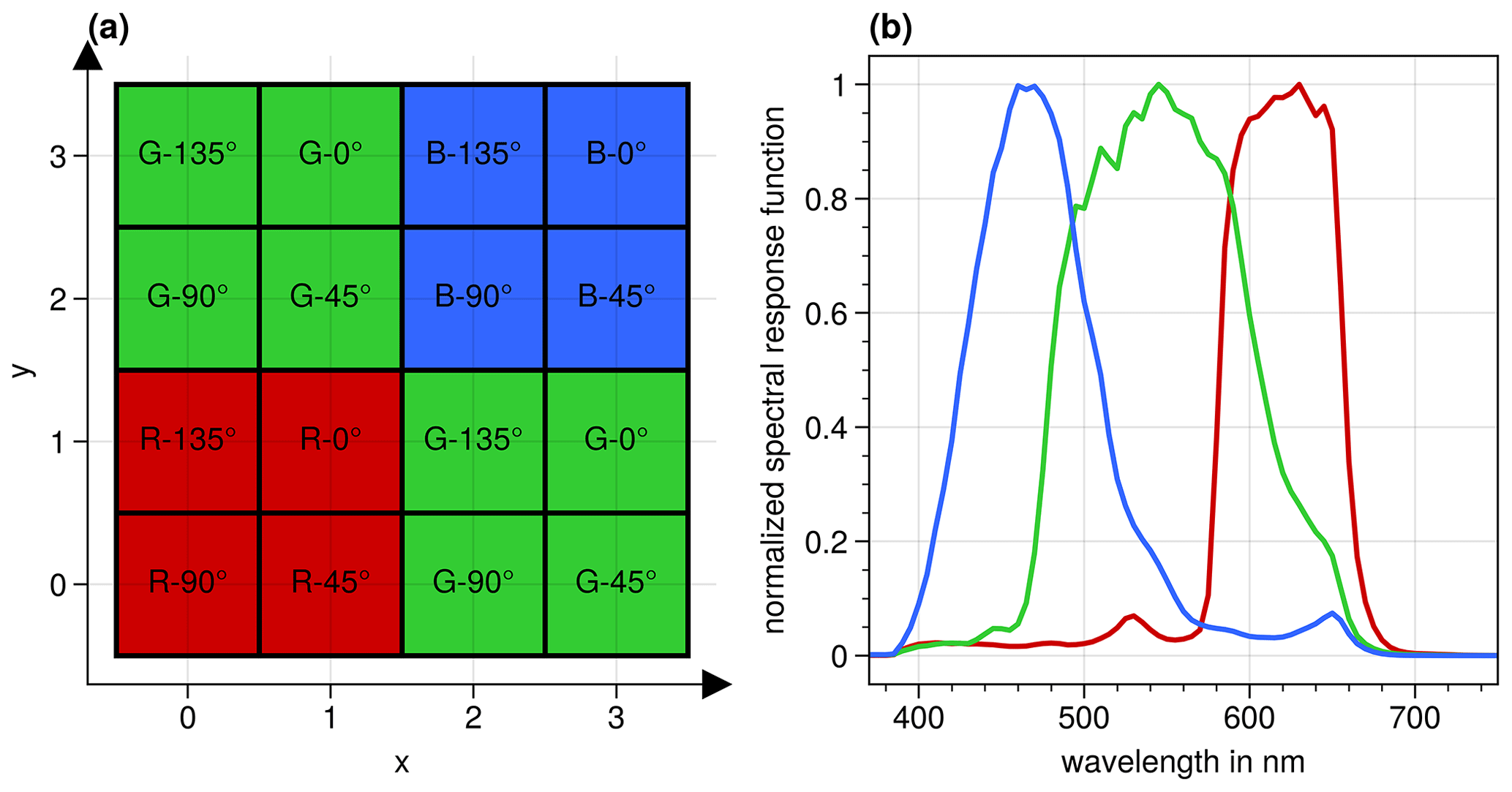
Figure 1(a) Structure of a 4 × 4 pixel block of the polarization cameras. Each 4 × 4 block is subdivided into four blocks of 2 × 2 pixels for the different colors: red (R), green (G), and blue (B). On the 2 × 2 pixel blocks, four differently angled polarizers are placed. Figure adapted from the datasheet of the camera (LUCID Vision Labs Inc., 2022a). (b) Normalized spectral response functions of the three color channels averaged over the four polarization directions, considering the effect of the camera lens and of the window of the specMACS housing on the spectral response function.
Figure 2 displays a specMACS measurement from 2 February 2020. Panels a and b show the measurements of the polA camera, which observes clouds slightly to the left in the flight direction, and panels c and d correspond to the polB camera, which observes clouds to the right in the flight direction. Figure 2a and c show the measured total intensities of the two cameras. Dashed lines indicate lines of constant scattering angle. The corresponding DOLP is shown in Fig. 2b and d. Most parts of the measurement have a small DOLP (dark in the image). The cloudbow region (scattering angle 135 to 165∘) and the backscatter glory (scattering angle 170 to 180∘) stand out due to their high DOLP. To avoid interpolation errors, we use the original data from the two individual cameras here, instead of projecting the data onto a common mapping/figure.
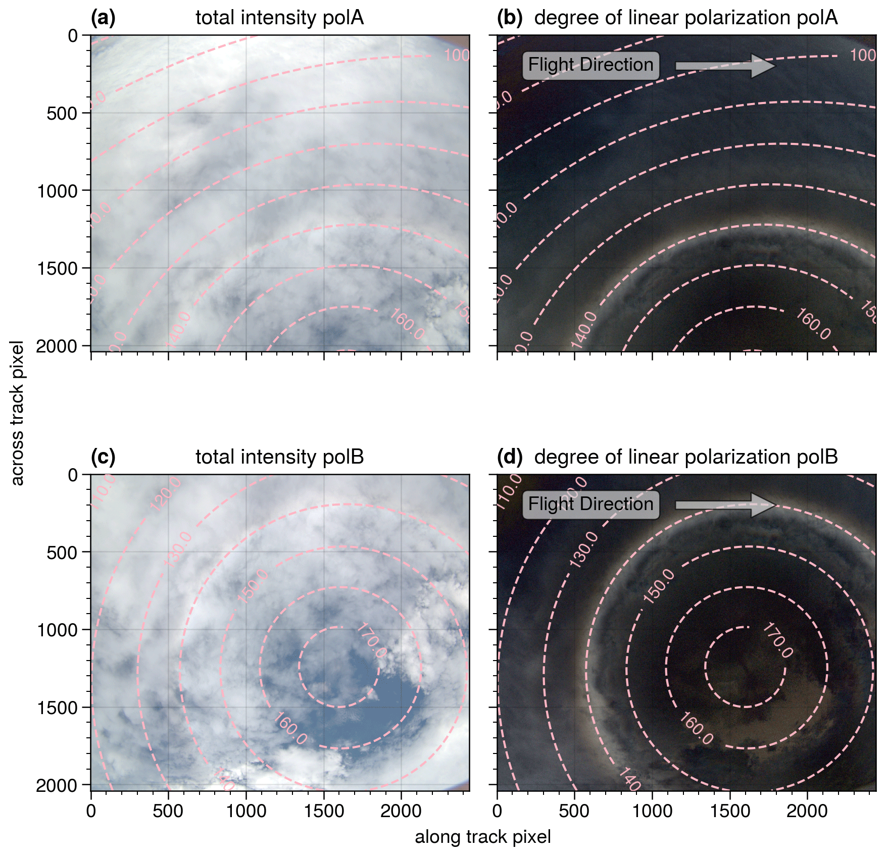
Figure 2Example of measurements of both polarization cameras (2 February 2020, 16:47:45.07 UTC): (a, b) measurements from the first polarization camera (polA), which looks slightly to the left in the flight direction; (c, d) measurements from the second polarization camera (polB), which looks slightly to the right in the flight direction. The field of view of the two cameras overlaps. Panels (a) and (c) show the total intensity, and panels (b) and (d) show the DOLP. The dashed lines indicate lines of constant scattering angles in degrees. The primary bow of the cloudbow is visible in the DOLP as a bright ring at a scattering angle of about 140∘.
A Stokes vector is defined with respect to a plane of reference. Often, the scattering plane, which contains both the incoming solar illumination vector and the view vector, is used as a reference plane (e.g., Eshelman and Shaw, 2019). This has the advantage that U≈0 within the scattering plane and Q contains all information about the polarized signal. In the case of the measurements, the original reference plane is the x–z plane of the camera coordinate system. The x axis of the camera coordinate system points in the flight direction, which is also the polarizing axis of the 0∘ filter. The z axis points in the direction of the optical axis of the camera. For further analysis, each measured Stokes vector is rotated into its scattering plane which is unique for each pixel (Hansen and Travis, 1974; Eshelman and Shaw, 2019), and we only evaluate Q. The window in front of the polarization cameras affects the polarization state of the measurements. To correct for this effect, the window is handled as a linear diattenuator, and the Müller matrix of a linear diattenuator is applied to the measurements (Bass et al., 1995).
A geometric calibration of the cameras was carried out using the chessboard calibration method described in Kölling et al. (2019) based on Zhang (2000), but we exchanged the thin prism model used in Kölling et al. (2019) with the rational model. Both camera models come from the OpenCV library (Bradski, 2000). In order to calculate the pixel coordinates of specific 3-D points, the location and orientation of the camera with respect to a fixed world coordinate system have to be determined. The required precise information about the position and attitude of the aircraft is part of the Basic HALO Measurement and Sensor system (BAHAMAS) dataset. A high-precision inertial reference system aided by data from a Global Navigation Satellite System (GNSS) delivers the data at 100 Hz. The accuracy of the data is further increased by GNSS post-processing after the flight (Giez et al., 2021). The camera location and orientation relative to the airframe is determined from the measured aircraft position and the location of distinct features, like rivers or roads, in the images once after installation.
The goal of our algorithm is to determine the size distribution of cloud droplets from angularly resolved cloudbow measurements. An average cloudbow signal could be extracted from a cross section of a single measurement (e.g., from Fig. 2). This method can easily be applied to any cloudbow observations, including those from commercial cameras, but the signal comes from a large area. The method presented in this paper is based on co-located along-track observations, allowing for the acquisition of the cloudbow signature of individual targets. As a result, distributions are obtained at a high spatial resolution, as this method does not involve averaging over a large area. With HALO, we fly over the clouds at a speed of about 200 m s−1, observing the same cloud from different viewing directions. Instead of evaluating the cloudbow in individual images, different viewing directions are sampled for each target on the cloud as specMACS images the scene (illustrated in Fig. 3). Similar approaches have also been applied to measurements of other airborne and spaceborne instruments (e.g., Bréon and Goloub, 1998; Alexandrov et al., 2015; McBride et al., 2020). The retrieval consists of three steps. First, cloud surface locations (“cloud targets”) in the real-world 3-D space and their trajectory caused by the wind are determined. For this purpose, we combine each 10×10 block of pixels from the specMACS images into target pixels. Such a target pixel typically has a size of about 100 m×100 m, but the actual size depends on the distance to the cloud. We decided to use this target pixel size because it matches our pointing accuracy. Second, for each cloud target, the pixels of all images observing that location are collected. The individual measurements of one target are aggregated into a combined radiance measurement for the entire range of the viewing directions. In a final step, a lookup table (LUT) based on Mie calculations of polarized phase functions for different DSD values is fitted to the angular distributions to retrieve the best-fitting DSD values. The particular steps of the aggregation process and the retrieval are described in the following.
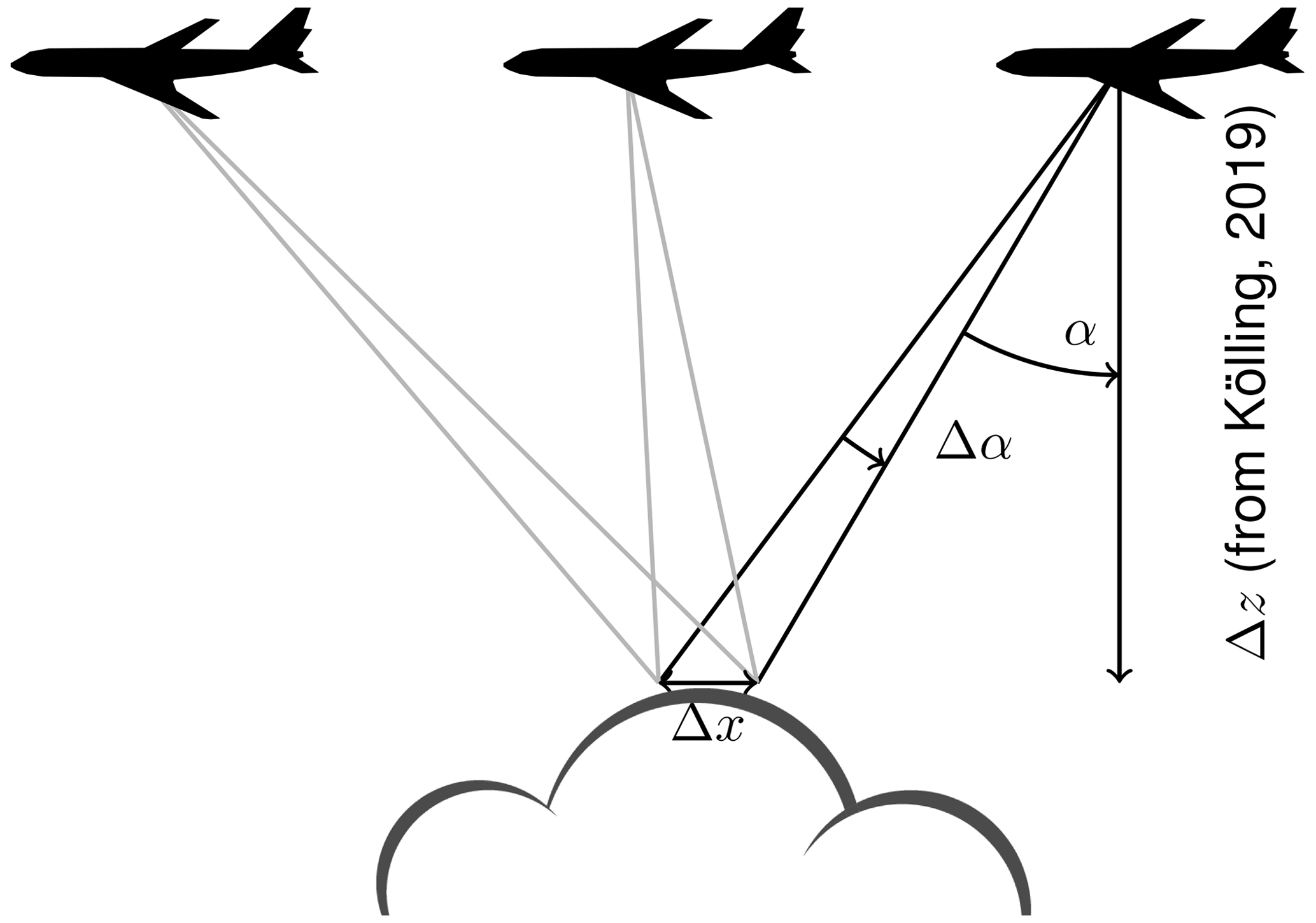
Figure 3Observation geometry: the same target on the cloud (indicated by Δx) is observed from different viewing angles (α). The cloud top height information needed to calculate the distance Δz between the target and camera is retrieved using the method described in Kölling et al. (2019). The single measurements are then aggregated into one radiance measurement of the target.
3.1 Cloud detection
The first step of the algorithm consists of detecting clouds in the measurements. As most measurements were taken above the ocean, the measurements are often contaminated with sunglint, which appears due to the specular reflection of sunlight by the ocean. Cloud detection algorithms based on the brightness of the image often wrongly identify this bright sunglint as clouds. To (partially) overcome this problem, we use the parallel component of the polarized light for cloud detection. In the parallel component, the reflectance of the sunglint is significantly reduced. At the Brewster angle ( for an air–water interface) reflected light is even completely perpendicularly polarized (Bass et al., 1995). In the case of a scene with medium cloud coverage, the algorithm chooses the red channel of the parallel component for further processing. For scenes with high cloud coverage, the normalized red (r) to blue (b) ratio (nrbr ) is calculated. Based on a brightness histogram of the selected data, a threshold value that distinguishes between cloudy and cloud-free pixels is determined using the method described in Otsu (1979).
A cloudy pixel is suitable for the cloudbow algorithm if it is observed within all scattering angles from 135 to 165∘ during the measurement sequence (for the choice of the range, see, e.g., Alexandrov et al., 2012a, or McBride et al., 2020). This, of course, depends on the solar geometry and the camera's viewing direction. Therefore, the next step is to identify the cloud targets that meet this criterion. In the case of Fig. 2, the upper part of the measurement cannot be used for the cloudbow retrieval, as these clouds are not observed from the full scattering angle range needed while the aircraft is flying above the cloud. The flight direction is to the right, as indicated by the arrow in Fig. 2, and the scattering angles are shown as dashed circular lines.
3.2 Geolocalization of cloud targets
In order to identify the same target in different observations, we first use the geometric calibration of the camera to determine the viewing angle of the target (see Sect. 2). To fully localize the target, we need to know the distance between the aircraft and the target (Δz in Fig. 3). The altitude of the aircraft and, thus, of the camera is measured by the BAHAMAS system. The cloud top height is derived using a stereographic reconstruction method which determines the cloud geometry from specMACS measurements. This was demonstrated for measurements of the previous 2-D RGB camera in Kölling et al. (2019). The method identifies pixels with prominent features that are detected in the following images by a matching contrast. To correct for horizontal displacements of the cloud, the method was extended to include data on the horizontal wind from the ERA5 reanalysis dataset (Hersbach et al., 2020, 2018). The dataset has an hourly temporal resolution, a 0.25∘ × 0.25∘ horizontal resolution, and 37 vertical levels from the surface to 1 hPa. During EUREC4A, clouds were typically observed at a vertical altitude of 1–2 km, where the ERA5 dataset has a vertical grid spacing of about 250 m. First, the stereo method is performed without additional wind information, and the 3-D coordinates of the identified pixels (stereo points) are retrieved. The ERA5 data are then interpolated to these coordinates to extract the corresponding wind data. The stereo method is performed again, but this time the wind data are taken into account. The whole process is iteratively repeated five times; each time the wind data are updated with the ERA5 wind interpolated to the heights and locations of the previously found stereo points. Further increasing the number of iterations did not notably change the results.
Figure 4a shows an example of the derived cloud top height of the polB camera using the stereographic method for the scene shown in Fig. 2c and d (2 February 2020, 16:47:45 UTC). Although the method has difficulties in inhomogeneous regions of the cloud due to a lack of contrast (e.g., in the lower right), large parts of the cloud are analyzed successfully. The cloud top heights from the single points of the stereographic method are interpolated to the entire image (Fig. 4c). The interpolation process first consists of a linear interpolation of the stereo pixels onto all image pixels inside the convex hull of the stereo pixels. Then, the regions outside the convex hull of the original stereo points are filled by a nearest-neighbor interpolation. The resulting cloud top heights are assigned to the selected cloud targets.
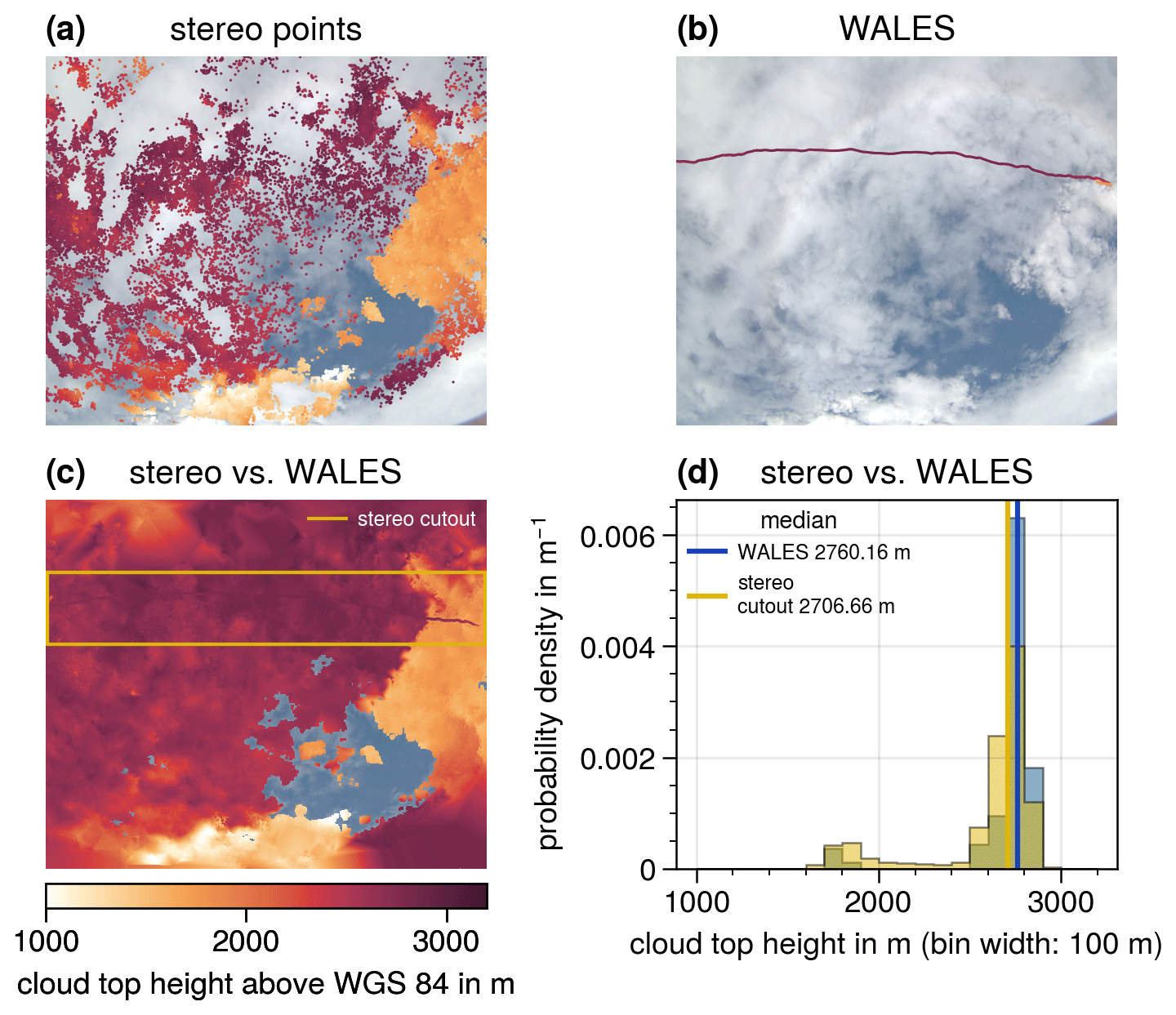
Figure 4Cloud top height (CTH) information of the cloud field shown in Fig. 2 (2 February 2020, 16:47:45.07 UTC). Panel (a) shows the CTH of stereo points from the stereographic reconstruction method, panel (b) presents the CTH from the WAter vapour Lidar Experiment in Space (WALES) lidar system, and panel (c) shows the interpolated CTH based on the stereo points. The WALES CTH is plotted on top (hardly visible due to the similarity to the CTH from the stereo points). The stripe marked by the yellow lines indicates a specMACS cutout surrounding the WALES track. Panel (d) shows the probability densities of the CTHs of the specMACS cutout (yellow) and the WALES measurements (blue). The RGB measurement of the cloud field is shown in the background of panels (a), (b), and (c). The color bar below panel (c) corresponds to all cloud top height measurements shown in panels (a), (b), and (c).
The WAter vapour Lidar Experiment in Space (WALES) lidar system was also operated aboard HALO during EUREC4A (Wirth et al., 2009; Konow et al., 2021). The stereographically derived cloud top height is very similar to the measured cloud top height from the WALES lidar (Wirth, 2021) which is projected onto the specMACS RGB image in Fig. 4b. Figure 4c plots the WALES track on top of the interpolated specMACS cloud top height map. Within the high cloud on the left, the WALES data agree very well with the specMACS cloud top height, and it is hard to distinguish the WALES data from the stereo data. The two datasets differ for the cloud on the right, where the stereo result is approximately 1000 m lower than the lidar measurement. From the videos of the specMACS measurements, it can be seen that the two cloud layers slightly overlap here. specMACS detects the lower cloud layer due to greater contrasts, whereas WALES is sensitive to the upper cloud layer. This behavior was also observed in Kölling et al. (2019). The stripe marked by the yellow lines in Fig. 4c roughly surrounds the WALES track and defines the area for which the yellow histogram in Fig. 4d is derived. The cloud top heights of the two respective cloud layers are at approximately 2700 and 1700 m (Fig. 4d). The distribution of the interpolated stereo points is quite similar to the distribution of the WALES data (shown in blue), even though the two datasets differ for the cloud on the right.
Even a small error of a few hundred meters in the cloud top height will result in an erroneous localization of the cloud in subsequent images. An incorrect localization particularly affects targets close to cloud edges, where it will cause non-cloud regions to be aggregated into the final cloudbow signal. Luckily, the stereographic method can very accurately determine the cloud geometry at cloud edges due to high contrasts.
By combining the cloud top height with the viewing directions, the locations of the cloud targets in the real-world 3-D space are determined. These are used to calculate the pixel coordinates of the targets in successive measurements (Fig. 3), again considering the shift in the targets with the wind. The individual measurements of the same target of the Stokes parameter Q are combined to generate the aggregated polarized radiance measurement. For further processing, the aggregated measurement is binned onto a scattering angle grid with a step size of 0.3∘. It should be noted that, although specMACS has two polarization cameras with a partly overlapping field of view, we have not combined the measurements of the two cameras to date. The results that are presented in the following are based on measurements of only one camera.
3.3 Size distribution retrieval
Polarized measurements are dominated by single scattering (Hansen, 1971). In general, any scattering process is described by the scattering matrix or phase matrix that relates incident to scattered radiation (Hansen and Travis, 1974). The scattering matrix is a 4×4 matrix with matrix elements Pij. The P12 element is also called the polarized phase function and is approximately proportional to the measured polarized radiance Q in the scattering plane (Bréon and Goloub, 1998). Under the assumption of single scattering, it is true that P12 is directly proportional to Q in the scattering plane.
Figure 5 shows examples of the polarized phase function for different reff (panel a) and different veff (panel b). This figure illustrates how the properties of the cloud droplets determine the shape and structure of the phase function and, thus, the radiance within the cloudbow and glory region. The position of the maxima and minima of the polarized phase function strongly depends on the reff (panel a). The veff, however, determines the amplitude and widths of secondary minima of the radiance distribution but has only a small effect on the position of the minima. Analyzing the backscatter glory is an extremely accurate method to retrieve reff and veff (Spinhirne and Nakajima, 1994; Mayer et al., 2004). However, the glory requires a special observation geometry and can, therefore, only be evaluated for a small fraction of the image area. The cloudbow, in contrast, covers a large area and, thus, is easier to observe, while still depending strongly on the size distribution.

Figure 5Panel (a) shows that the cloudbow signals (P12) vary if the reff is changed while the veff is constant (veff=0.08). Panel (b) illustrates the effect of a change in the veff while the reff is held constant (reff=4.89 µm). For calculating P12, we assume that the DSD has the shape of a gamma distribution. The P12 curves shown here are for the green channel of the specMACS cameras. In panels (c) and (d), several gamma distributions for different veff and a constant reff=10 µm (c) and for different reff and a constant veff=0.1 (d) are shown.
For evaluating the aggregated angular radiance measurement with regard to the cloud droplet size properties (see Fig. 5), a LUT of polarized phase functions (P12) for different reff and different veff was created for each of the three spectral color channels of the camera. All calculations were carried out with the Mie tool of the library for radiative transfer (libRadtran) (Wiscombe, 1980; Mayer and Kylling, 2005; Emde et al., 2010, 2016). We assume that the DSD has the shape of a monomodal gamma distribution. This is an extensively used assumption (Alexandrov et al., 2015) that is, for example, confirmed by in situ measurements of liquid water DSDs (e.g., Miles et al., 2000). The reff and the veff of any DSD are defined as follows (Hansen, 1971):
-
effective radius,
-
effective variance,
Here, r is the droplet radius, and n(r) is the DSD. The formula of the gamma distribution can be written as a function of reff and veff (Hansen, 1971):
where
Here, N is the total number of particles per unit volume. In Fig. 5, several gamma distributions for different veff (panel c) and reff (panel d) are shown.
Polarized phase functions are calculated for a logarithmic grid of 77 different reff ranging from 1 to 40 µm (). The veff range between 0.01 and 0.325, with a small step size of 0.01 for veff≤0.05 and a larger step size (0.02 to 0.028) for veff>0.05. This choice is similar to other publications, such as Alexandrov et al. (2012a) and McBride et al. (2020). In total, the LUT includes 16 different veff. To account for the different spectral sensitivities of the three color channels, the polarized phase functions are initially calculated for the whole wavelength range of the spectral response functions with a step size of 10 nm and are then weighted by each spectral response function (Fig. 1b). For the calculation of the phase functions, a wavelength- and temperature-dependent refractive index is used. We use the approximation formula of the IAPWS (International Association for the Properties of Water and Steam; Wagner and Pruß, 2002) for a temperature of , which, according to dropsonde measurements, corresponds to the approximate cloud top temperature of the typical EUREC4A clouds with a cloud top height of 1700 m.
The LUT of polarized phase functions (P12[reff,veff]) is fitted to the aggregated radiance distributions (Qmeas) using the following equation:
Here, A, B, and C are fitting parameters, and θ is the scattering angle. Parameter A is needed to compare the radiometrically uncalibrated measurements with the simulated LUT, and, in addition, it scales with the cloud fraction of the target made up of 10×10 pixels (Bréon and Goloub, 1998). The fitting parameters B and C account for any remaining effects that are not considered in the single-scattering assumption. For example, these could be contributions by multiple scattering. The term cos 2(θ) corrects for Rayleigh-scattering contributions (Alexandrov et al., 2012a). Other studies do not rely on the cosine term and instead use a correction term linear in θ plus a constant (e.g., Bréon and Goloub, 1998; Bréon and Doutriaux-Boucher, 2005). In the cloudbow range, however, this is similar to cos 2(θ) (Alexandrov et al., 2012a). A further contribution, beyond single scattering, could be a thin cirrus cloud above the cloud that generates the cloudbow. In Riedi et al. (2010), it was shown that the polarization signal of ice particles depends linearly on the scattering angle in the rainbow region. Furthermore, Alexandrov et al. (2012a) showed that the magnitude of a cloudbow signal is attenuated by an overlying aerosol layer, but the aerosol layer does not change the structure of the cloudbow signal. The fitting parameters B and C also account for these two effects of cirrus and aerosols.
To determine P12 (and thus the reff and veff of the DSD), a least-squares approach is used to invert Eq. (6). In the inversion process, not only the grid points of the LUT are allowed but also values in between. This is realized by a linear interpolation of the LUT. The root-mean-square error (RMSE) is calculated for the scattering angle range from 135 to 165∘ where the cloudbow structure is most prominent:
The smallest RMSE reveals the reff and veff of the DSD. In addition, the RMSE serves as a measure of accuracy, and we filter out all fits with RMSE>2.5. As a second quality measure, we calculate the quality index “Qual”, as in Eq. (8) (first defined by Bréon and Doutriaux-Boucher, 2005). This is the ratio between the variability in the measurement, which corresponds to the squared amplitude of the cloudbow (A⋅P12), and the RMSE of the fit. Measurements with a low quality index (Qual<4) are filtered out of any further processing. This excludes, for example, “cloudbow signals” of ocean areas that have been incorrectly identified as clouds from the result.
Figure 6 shows two examples of aggregated cloudbow measurements for the green channel binned into a 0.3∘ resolution in the scattering angle (black dots with standard deviation and connecting black line). Each corresponding model fit is plotted as a solid yellow line. The model fit matching the example shown in Fig. 6a has reff=17.63 µm and veff=0.08. The example in Fig. 6b has reff=5.98 µm and veff=0.08.
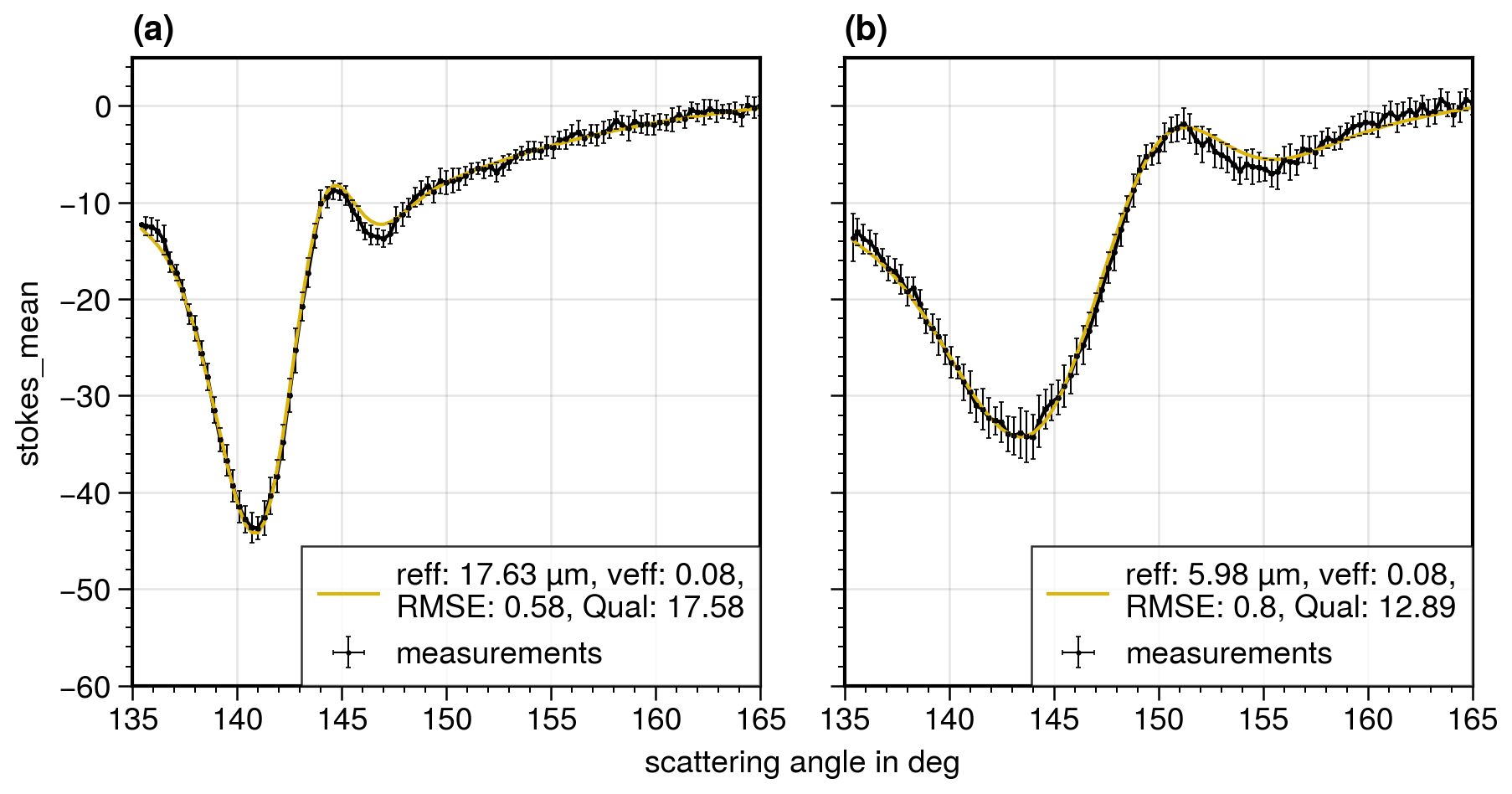
Figure 6(a, b) The aggregated polarized radiance measurements of the green channel of two different target regions. The raw data are binned to a 0.3∘ resolution in the scattering angle (black dots connected by black lines). The error bars represent the standard deviations of all original data points within a 0.3∘ bin. The yellow lines indicate the best-fitting simulations. The parameters reff, veff, RMSE, and Qual of the best-fitting simulations are shown in the boxes in the lower right.
In the following, two case studies from 2 February 2020 are presented. On this day, the observed clouds had a clear flower organization (Stevens et al., 2020; Dauhut et al., 2022). Such cloud fields are characterized by shallow trade-wind cumuli organized into large stratiform clusters (20–200 km) with high rain rates and surrounded by a large clear-sky region (Stevens et al., 2020; Schulz et al., 2021). Among the four named mesoscale trade-wind cloud patterns (flower, gravel, fish, and sugar), the flower clouds have the highest cloud radiative effect (Bony et al., 2020), mostly because of their large low-level-cloud fraction. We demonstrate the polarimetric technique based on two case studies from specMACS measurements of this day. The first case study shows a part of the (stratiform) flower structure. In the second example, we analyze small trade-wind cumuli that were connected to a cold pool that formed during the dissipation of the flower. We limit the presentation of the retrieval results to the green channel, as the results from the red and blue channels are very similar.
4.1 Case study 1 – stratocumulus flower-cloud system
First, we present the flower cloud observed at 16:47:45 UTC. This measurement has already been introduced in Sect. 3 and is shown in Fig. 2. At this time, HALO was flying at an altitude of about 10 km, and the solar zenith angle was 31.15∘. The cloudbow technique is applied to the measurements. The time required to sample the angular range from 135 to 165∘ is 40 s. Figure 7g shows the RGB image of the measurement from the polB camera. The labels on the four sides of the image indicate the distances between the neighboring corners of the image. It is noticeable that the side lengths of the top (14.44 km) and bottom (27.02 km) differ greatly. This happens because the camera is installed at a slight angle in the across-track direction; therefore, the lower part of the image covers a much larger distance in the along-track direction. This is also the case for the measurements of the polA camera, but the upper part of the image covers a larger distance here. The retrieval results of the individual cloud targets are combined into maps of reff and veff (Fig. 7a and b, respectively). About one-third of the image can be evaluated, as only the targets inside this area are observed from all necessary scattering angles during the overpass. The map of reff (Fig. 7a) is a consequence of the vertical distribution of the cloud field with two cloud layers at different cloud top heights (Fig. 4 and Fig. 7h). The upper cloud deck at a height of about 2700 m has a large reff ranging between 15 and 40 µm. Distinct patches of very large reff values up to 40 µm are observed. These patches occur in regions where the cloud is optically thick (Fig. 7g). The spatial distribution of reff for the lower cloud deck (cloud top height of 1700 m) is more homogeneous, and the absolute values are much smaller (reff≈6 µm). Figure 7d shows the frequency distribution of reff, and the two reff peaks of the two cloud decks are very easily distinguished.

Figure 7Spatial distributions of reff (a), veff (b), and RMSE (c) for the case study presented in Fig. 2. Panels (d)–(f) show the corresponding frequency distributions. Panel (g) shows the RGB image of the measurement. The labels on the four sides of the RGB image indicate the distances between neighboring corners of the image. Panel (h) shows the cloud top height from the stereo method interpolated onto the whole pixel grid of the image. Three specific cloud targets are indicated by colored circles on the maps.
The retrieved reff values of the higher cloud are very large. To better understand the cloud field and the large reff values, we looked at radar measurements of the polarimetric Ka-band MIRA-35 cloud radar of the HAMP (HALO Microwave Package) instrument aboard HALO (Mech et al., 2014; Konow et al., 2021). The radar measurements from 16:47:00 to 16:48:30 UTC are shown in Fig. 8 as well as a push-broom-like image of the specMACS measurements and an indication of the HAMP radar field of view within the specMACS image. Within the high cloud from 16:47:00 to 16:48:15 the radar shows bands of enhanced reflectivity >0 dBz and positive fall speeds (not shown). This likely corresponds to sedimenting droplets. Along with our observation of droplet sizes clearly larger than the usual cloud droplet size range (<15 µm), this points to drizzle development, and we may see impacts of precipitation formation deeper in the cloud within the polarimetric signal originating from cloud top. Although our technique is not able to observe the precipitation droplet range (>100 µm) directly, it is still sensitive to the intermediate size range below a possible drizzle droplet mode. This case study is particularly interesting, as the retrieved reff values lie within the size gap where neither the diffusional growth nor growth by collision–coalescence is effective (Grabowski and Wang, 2013). A recent study by Sinclair et al. (2021) discussed the correlation between large cloud droplets detected by the RSP polarimeter and rain observed with a radar in great detail and found that the estimated cloud top precipitation rates are strongly correlated with radar-derived precipitation rates and rainwater paths.
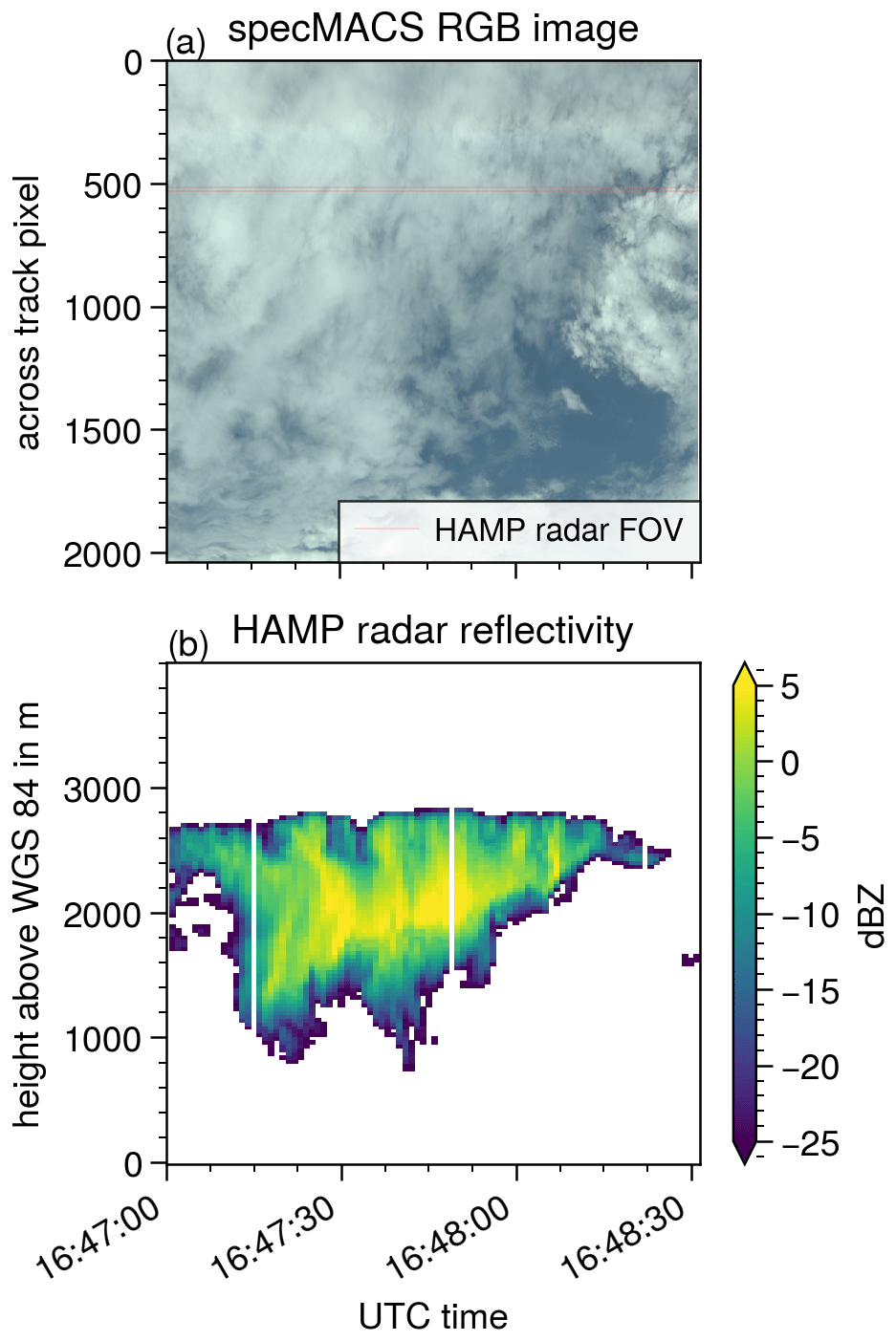
Figure 8Temporal evolution of specMACS measurement (a) and HAMP radar reflectivity (b) for case study 1. The specMACS measurements are stacked together from individual images to generate a push-broom-like image with a time axis. The HAMP radar field of view is marked within the specMACS image.
For our polarimetric technique, it is necessary to make an assumption regarding the shape of the DSD. Currently, we use a monomodal gamma distribution for this purpose. In Alexandrov et al. (2012b), it was shown that the polarimetric retrieval based on monomodal DSDs is biased towards the dominant mode for clouds with a bimodal DSD (e.g., due to drizzle). To overcome this problem, the rainbow Fourier transformation (RFT) was developed, and it retrieves the DSD without any assumptions regarding the number of modes of the distribution (Alexandrov et al., 2012b). When comparing the polarimetric technique to the traditional bispectral retrieval, it should be noted that bispectral retrievals are (normally) also based on simulations with monomodal DSDs (Platnick et al., 2017); this tends to underestimate the true reff and has been investigated in several studies (e.g., Zinner et al., 2010; Zhang et al., 2012; Zhang, 2013).
The spatial distribution of veff in Fig. 7b does not show a clear separation of the two cloud decks. Small patches of both very high and very low veff can be seen. At the boundary between the two cloud decks, large veff values are observed over several pixels. These are the result of a mixing of the signals of the two different cloud decks with different DSDs. Similar effects have been seen in RSP observations of multilayer clouds (Alexandrov et al., 2015, 2016). The resulting oscillating signal cannot be reproduced by a monomodal polarized phase function, and the outcoming fit has a large veff. The frequency distribution of veff is shown in Fig. 7e, and veff has a median value of 0.11.
Figure 7c and f show the spatial distribution and the frequency distribution of the RMSE. The RMSE has a median value of 0.85, and there is no noticeable difference between the RMSE of the lower cloud with small reff and the upper cloud with large reff. Small cracks are visible within the spatial distributions of reff, veff, and the RMSE due to the reprojection of the targets onto the RGB image of the measurement, as there are small discontinuities within the interpolated stereo cloud top height. This, in turn, results in discontinuities within the locations of the reprojected targets.
The maps in Fig. 7 contain indicators of three particular cloud targets (colored circles). For these targets, the respective aggregated cloudbow measurements are plotted together with the model fits in Fig. 9. Targets a and b both lie within the high cloud deck. Target a is located within a patch of very high reff. The corresponding cloudbow measurement has one very sharp minimum as well as a second weaker minimum. This indicates a relatively broad DSD. This is confirmed by the quite large veff value of 0.16. The measurement of target b has several secondary minima. Therefore, veff is reduced compared with target a (veff=0.02). Target c lies within the lower cloud deck. The cloudbow minimum is shifted to slightly larger scattering angles, and the amplitude of the cloudbow is smaller than the amplitudes of targets a and b. According to our expectations from the simulations (Fig. 5), this corresponds to a smaller reff, which is confirmed by the fit (reff=8.68 µm). The existence of the secondary minima indicates a narrow size distribution which is verified by the small veff of the fit (veff=0.02). All three measurements have little noise indicated by the error bars.
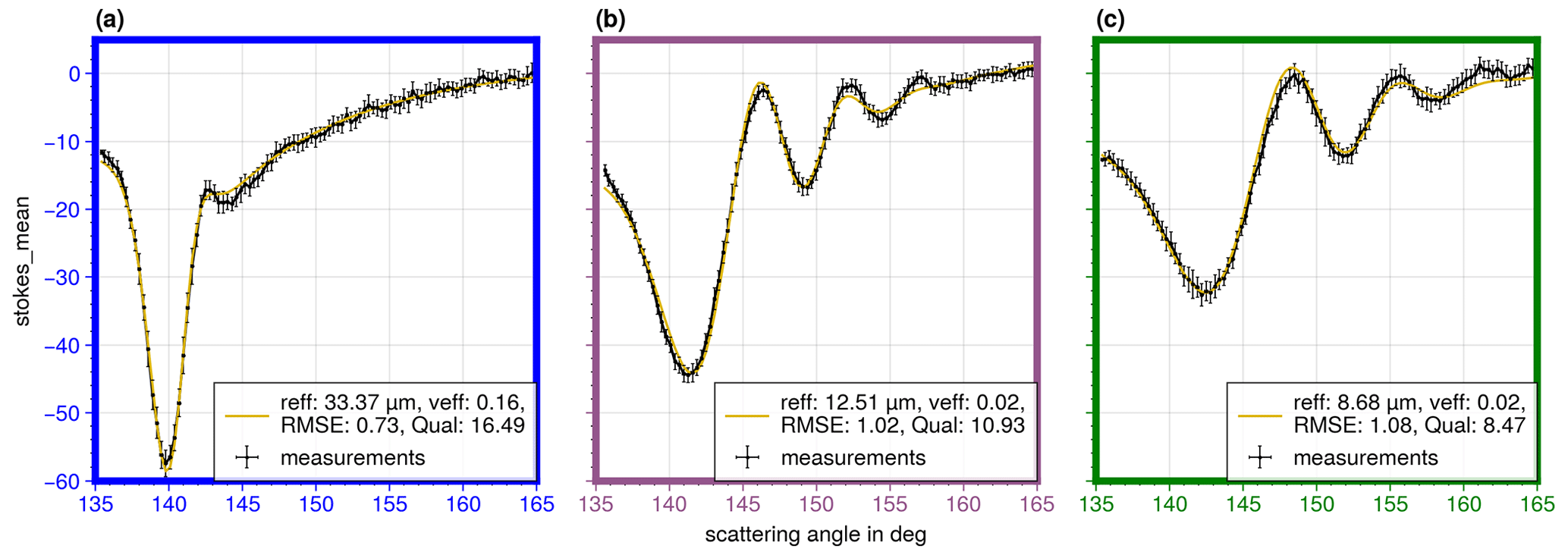
Figure 9The aggregated polarized radiance measurements of the green channel of the locations shown in Fig. 7 were binned to a 0.3∘ resolution in the scattering angle (black dots connected by black lines). The error bars represent the standard deviations of all original data points within a 0.3∘ bin. The yellow lines indicate the best-fitting simulations. The parameters reff, veff, RMSE, and Qual of the best-fitting simulations are shown in the boxes in the lower right.
4.2 Case study 2 – small cumulus clouds
In the following subsection, a second case study is discussed. The observations were taken from 18:28:15 to 18:31:30 UTC with the polB camera. HALO was flying at an altitude of 10 345 m, and the solar zenith angle was 46.1∘. The measurement shows a cloud field of small trade-wind cumulus clouds with diameters of about 1–2 km (Fig. 10b). We choose this example to demonstrate that the retrieval is capable of generating good results, even in the case of more heterogeneous cloud scenes and especially for small cumulus clouds. In such scenes, the traditional bispectral retrieval has issues with 3-D radiative transfer effects (Marshak et al., 2006; Zhang et al., 2012). These are shadowing or illumination effects, which are normally not accounted for in standard radiance lookup tables.
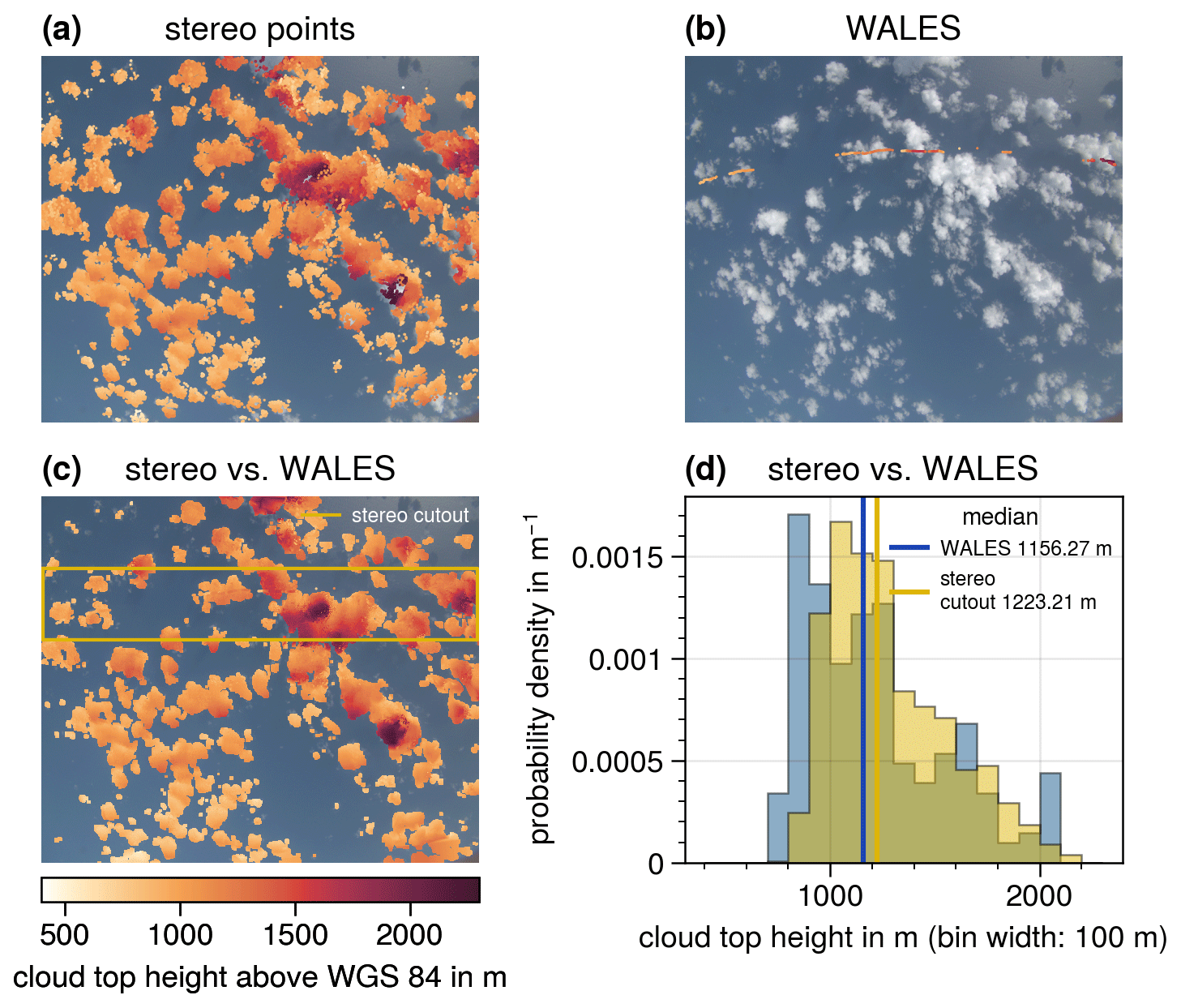
Figure 10Cloud top height (CTH) data of the case study of small cumulus clouds (2 February 2020, 18:29:30 UTC). Panel (a) shows the CTH of stereo points from the stereographic reconstruction method, panel (b) presents the CTH from the WALES lidar system, and panel (c) shows the interpolated CTH based on the stereo points. The WALES CTH is plotted on top. The stripe marked by the yellow lines indicates a specMACS cutout surrounding the WALES track. Panel (d) shows the probability densities of the CTHs of the specMACS cutout (yellow) and the WALES measurements (blue). The RGB measurement of the cloud field is shown in the background of panels (a), (b), and (c). The color bar below panel (c) corresponds to all cloud top height measurements shown in panels (a), (b), and (c).
In the case of small cumulus clouds, a precise geolocalization is important for image-to-image tracking. This geolocalization depends on three factors: the internal calibration of the camera, the (mainly horizontal) wind at the cloud top, and the retrieved cloud top height. In the following, we argue that, while these points certainly cause uncertainty in the geolocalization, they affect the cloudbow retrieval to a lesser degree.
The internal calibration was verified using known targets at the ground. A slight deviation from the actual target of less than 100 m was observed, which also varied during the overflight. A possible reason for a slightly varying offset could be a degrading heading accuracy of the inertial reference system on long, straight flight legs with no heading variation (Giez et al., 2021). As most of the EUREC4A flights were conducted using a circular flight pattern, the heading of the aircraft continuously changed, and the accuracy of the position and attitude data is very high. As the inertial reference system is located in the nose of the aircraft and the specMACS system in the tail, deformation of the fuselage caused by air turbulence or outside pressure change could also induce a varying offset in the pointing accuracy. Other inaccuracies result from the geometric chessboard calibration of the cameras and from the determination of the correct position of the specMACS instrument relative to the airframe by aligning specMACS measurements with satellite imagery. Based on this analysis of known ground targets, we used cloud targets of approximately 100 m × 100 m in size in the current study. In the following, we will refer to this size of 100 m as “target unit”. Future work will address improving the geometric calibration of the cameras to allow the study of even smaller targets.
The second factor that affects the geolocalization is the ambient horizontal wind. We apply a wind correction to the initial location of the cloud target to account for any drift due to the wind; we explain why this is necessary in the following. According to the ERA5 data, the ambient horizontal wind of the case study at the cloud height (about 1 km) was an east-southeast wind (direction 103∘) with a wind speed of about 6 m s−1. This was also confirmed by dropsonde measurements. During the flight, it took about 35 s to sample the targets from the angular range of 135 to 165∘. During this aggregation process, a target cloud shifts by 210 m due to the wind. For a cloud target with a size of about 100 m × 100 m, this means that it moves further by more than two target units; therefore, a wind correction is required. In addition, a cloud can evolve significantly within 35 s, especially in the very active region at the cloud boundary, where the cloud grows or shrinks depending on cloud dynamics and the interaction with the environment.
The stereographic cloud geometry retrieval is very applicable to this cloud field because of the strong contrasts between the clouds and the ocean. The resulting cloud top height (shown in Fig. 10a) is relatively constant across the whole cloud field with a median value of about 1200 m. Some (diameter-wise) larger and more developed clouds also have higher cloud tops up to 2200 m. Cloud top height data derived from WALES lidar measurements are projected onto the specMACS RGB image and are shown in Fig. 10b. The lidar measurements are also plotted on top of the stereo points, which were interpolated onto the whole image (Fig. 10c). The stereographic result is again similar to the WALES measurements. This is also evident in Fig. 10d, where the probability density of the stereo data in the surroundings of the WALES track (yellow rectangle in Fig. 10c) is plotted along with the WALES cloud top height data (blue).
For a successful cloudbow retrieval, we rely on an accurate aggregation of the measurements by mapping from the known viewing angles to the image pixel location corresponding to the same cloud target. The stereographic approach of tracking cloud targets from one image frame to the next provides this precise information. It determines the cloud height by finding the ideal match between the known viewing directions during the overpass and the connecting line between identified targets at cloud top and the aircraft based on a matching contrast in different images. Some remaining residual/mispointing error in the tracking, which stems from error sources in the geometric calibration (and, as a result, in cloud top height and horizontal wind), has negligible effects on the tracking. We manually verified the tracking of cloud targets with distinctive features during the overflight. One such example is shown in Fig. 11. Based on the location of the targets and the ambient wind at 18:29:40 UTC (panel b), the pixel positions of the targets in a previous (panel a) and a later (panel c) image are calculated. A visual comparison of the identified targets in the different images shows that the targets are successfully tracked: the colored markers in Fig. 11 highlight the same areas of the cloud in all three images. Due to camera distortions, the originally rectangular cloud targets (at 18:29:40 UTC) increasingly take the shape of a trapezoid when they approach the edge of the entire image. Each panel in Fig. 11 shows only a small part of the entire image.
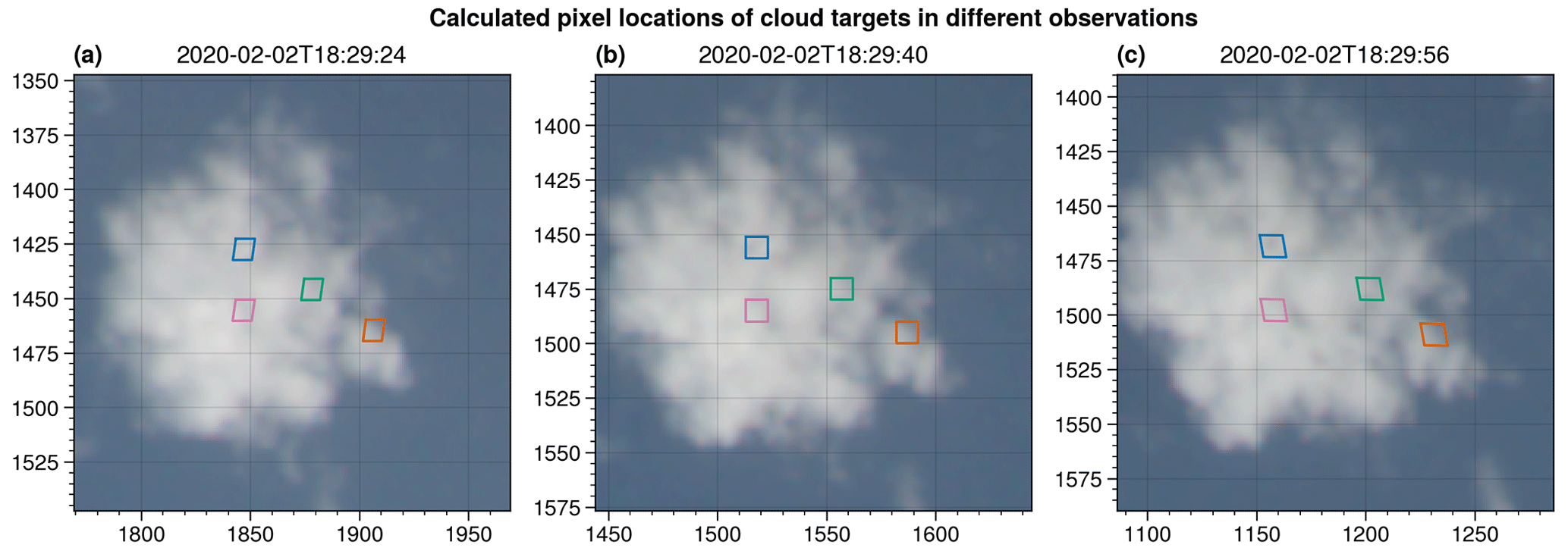
Figure 11Calculated pixel positions of cloud targets, indicated by different colors, in observations at different times during the overflight.
The retrieved reff, veff, and RMSE results are projected onto the RGB image and shown in Fig. 12a–c. The corresponding frequency distributions are shown in Fig. 12d–f. Figure 12g and h show the RGB image of the measurement as well as an indication of the dimension of the image and the interpolated cloud top height, respectively. Compared with case study 1, reff is much smaller (median of 7.0 µm) and has a more narrow distribution. Values of reff larger than 12 µm are not observed. The spatial distribution of reff is homogeneous and has few outliers. For higher cloud tops, an increase in reff is observed. This dependence of the reff on the cloud top height is presented in more detail in Fig. 13. Here, the derived reff of all individual clouds of the case study are plotted against the corresponding cloud top heights (as in Rosenfeld and Lensky, 1998). We refer to this plot as a vertical profile, although it does not show the actual reff profile within a single cloud. The idea is that the individual clouds of the cloud field are captured at different stages of their vertical growth. It is then assumed that the retrieved reff which is sampled at the cloud top is representative of the actual reff at the same height inside a single cloud. This assumption applies only to non-precipitating clouds. By combining the measurements of the individual clouds at different stages of their vertical development, a vertical profile is constructed, which is assumed to correspond to the vertical profile of a single growing cloud. Figure 13 shows a strong increase in reff from about 5 µm at a height of 800 m to 9 µm at 1350 m. This rapid growth of droplets with height may indicate the dominance of growth through coalescence and is typical of maritime clouds. Rosenfeld and Lensky (1998) refer to this zone as the “droplet coalescence growth zone”.

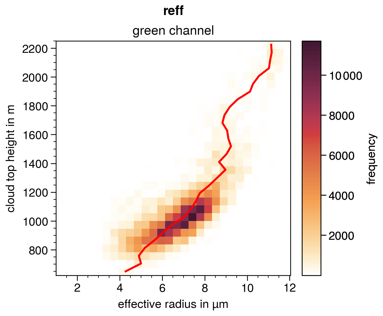
Figure 13Vertical profile of the retrieved reff of the cloud field shown in Fig. 12. The red line indicates the average reff for each vertical layer.
The veff (Fig. 12b and e) is small (median veff of 0.08) and consistent within the inner part of the clouds. There are some cloud targets with veff=0.32 (the upper limit of the LUT) that occur mainly at the edge of the cloud. Especially at the edge of the cloud, a small offset in the geolocation can have a significant impact on the aggregated observations. The offset between the assumed location and the actual location may increase during the aggregation process and could even include ocean measurements for targets at the cloud edge. In this case, the aggregated measurements originate from different targets, and the cloudbow signal broadens or vanishes completely. We tried to ensure that the RMSE and Qual criteria successfully filter out such cases. Furthermore, it could also be a physical effect related to entrainment and (inhomogeneous) mixing of dry air in the cloud. In this case, modeling studies predict a broadening (increase in veff) of the DSD (Pinsky et al., 2016). Such questions will be investigated in the future using the high-resolution specMACS data.
The black rectangle in Fig. 12 marks a single cloud (diameter of 1.5 km) that is presented in more detail in Fig. 14. In Fig. 14, maps of the reff, veff, and the cloud top height are shown along with the frequency distributions of reff and veff of the single cloud. The Qual and RMSE criteria filter out some of the cloud targets inside the cloud, which mainly appear in shadowed or optically thin parts of the cloud. The high spatial resolution of the measurements reveals small-scale structures of the DSD, especially regarding the veff, which is, for example, increased along a line from the top left to the center of the cloud. Three targets of the cloud are selected (marked by circles on the maps). Targets a and b have a similar reff but differ with respect to the veff. Target c lies within the region of increased cloud top height, where reff is also large. The difference in these three targets is visible in the aggregated cloudbow observations presented in Fig. 15, which especially vary regarding the number and visibility of secondary minima. The observations are more noisy compared with the observations of case study 1 (Fig. 9), and the absolute values of the cloudbow signals are also less strong. This indicates that, even within one target, the variability in the cloudbow signal is relatively large. A further reduction in the size of a target would be helpful, but this comes with the need for a further increase in the geolocalization precision. Although the observations are more noisy, the primary cloudbow is still very pronounced, indicating that the retrieval of reff is robust. Furthermore, reff is relatively small for all three targets (6.54–9.2 µm). In this size range, the cloudbow signal depends strongly on reff (see Fig. 5). The result of veff is more difficult to interpret. The structure of the supernumerary bows (which mainly defines veff) can become smoothed out while averaging the signals of different DSDs within the averaging target, and the resulting DSD is, in the worst-case, different from any of the actual sub-pixel distributions. A sensitivity analysis of the cloudbow algorithm based on different resolutions of AirHARP data was presented in McBride et al. (2020) to identify effects of sub-pixel variability. This analysis showed that, in the case of a wide spread of the DSDs within the sub-pixels, the coarse-resolution result may not reflect the mean of the sub-pixels, as the combination of different gamma size distributions from the sub-pixels is not another gamma size distribution (Shang et al., 2015). Furthermore, the AirHARP study used a single, constant cloud top height for the entire scene which introduces uncertainty in the retrieval (McBride et al., 2020). In the future, the specMACS retrieval will be applied to even smaller targets which will further reduce effects of sub-pixel variability.
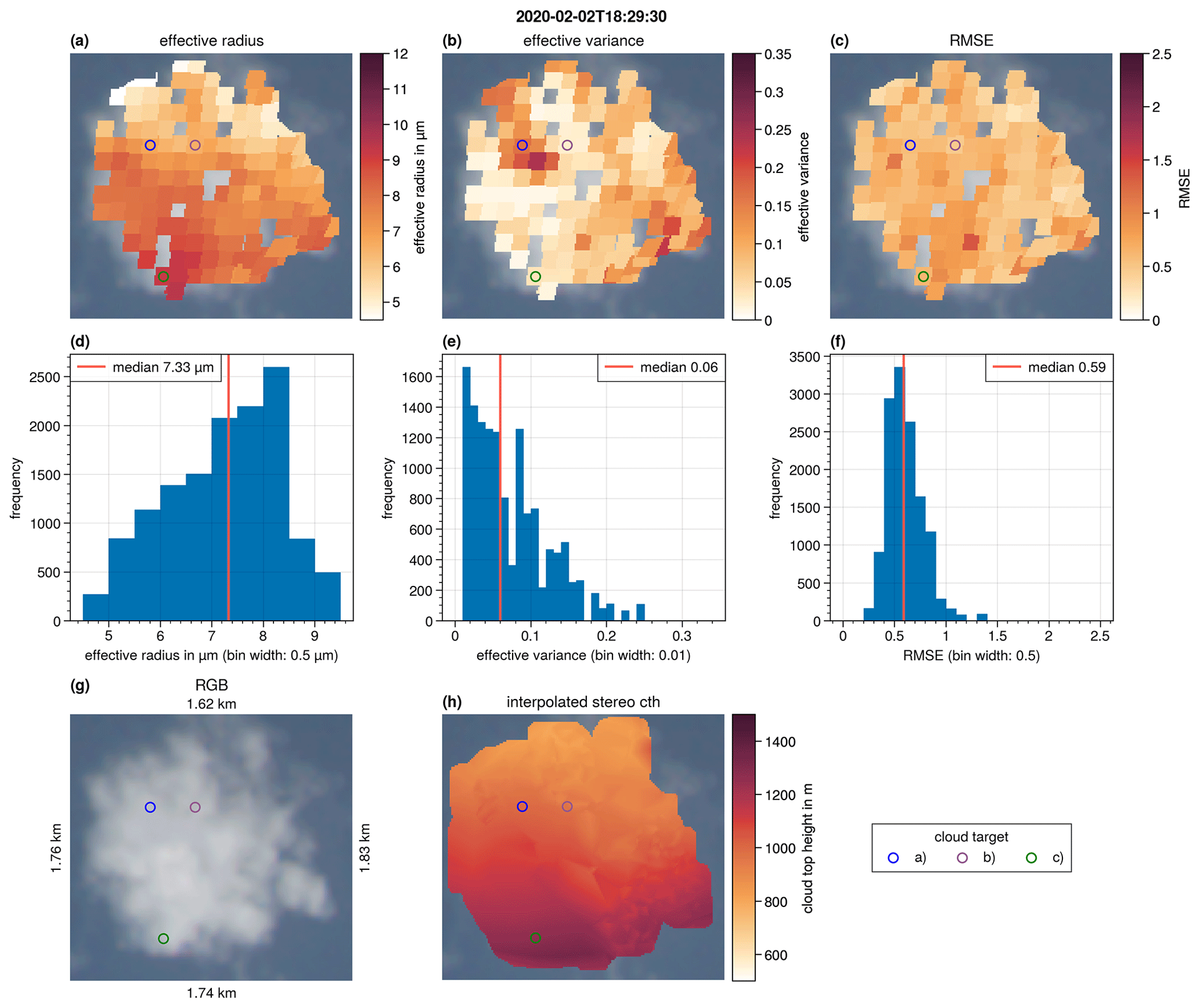
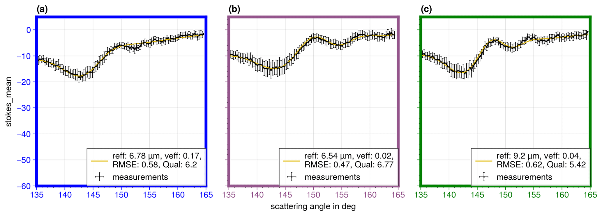
Figure 15The aggregated polarized radiance measurements of the green channel of the locations shown in Fig. 14 were binned to a 0.3∘ resolution in the scattering angle (black dots connected by black lines). The error bars represent the standard deviations of all original data points within a 0.3∘ bin. The yellow lines indicate the best-fitting simulations. The parameters reff, veff, RMSE, and Qual of the best-fitting simulations are shown in the boxes in the lower right. For better visual comparison with the aggregated measurements of the first case study, the y axis covers the same range as in Fig. 9.
We used the measurements of the new polarization-resolving cameras of specMACS to retrieve the reff and veff of the DSD at the cloud top. The method relies on polarized measurements of the cloudbow, which is sensitive to reff and veff. Cloud top height data from an existing stereographic retrieval (Kölling et al., 2019) are combined with the measured aircraft position and attitude data to geolocate the measurements. A parametric fit is applied to all data points that contain the full cloudbow signature (scattering angle 135–165∘). The results of the cloudbow retrieval are combined into spatial maps of reff and veff that give new insights into cloud microphysics and the spatial distribution of the parameters at the cloud top. The maps reveal structures within the cloud that may be linked to dynamic processes. We presented two case studies from the EUREC4A campaign. The first study shows a stratiform cloud with two (mostly nonoverlapping) cloud layers at different heights. In the higher cloud layer, large reff (25–40 µm) are retrieved. These values correlate with bands of high radar reflectivity values indicating sedimenting droplets. The spatial maps are rather smooth and have few outliers. The high spatial resolution of the retrieval results (currently about 100 m×100 m) allows the observation of small cumulus clouds, which can be evaluated accurately using the polarimetric cloudbow technique. This is demonstrated in the second case study which shows cumulus clouds with diameters of 1 to 2 km. The retrieved reff values are much smaller (3–12 µm) and the veff increases from the cloud center to the edge with a median value of 0.08. During EUREC4A, many similar cloud fields were observed. Further evaluations of such cloud fields will include studying the effect of entrainment and mixing processes on the DSD of small cumulus clouds in more detail. As the cloudbow is a single-scattering phenomenon, the results are less affected by 3-D radiative transfer effects, in contrast to bispectral retrievals that are not applicable to such small clouds.
In the past, similar methods have been applied to the measurements of other instruments such as POLDER, RSP, or AirHARP. To situate specMACS in the scope of the preexisting instruments, we summarize the main features of specMACS and compare them to the technical details of the RSP and the AirHARP instruments. The main differences between the instruments are listed in Table 1, based on Alexandrov et al. (2012a) and McBride et al. (2020). The outcome of all three instruments' retrieval techniques are angularly resolved measurements of the Stokes parameters: I, Q, and U. However, the way these measurements are generated differs:
-
Each observation of the specMACS instrument is a 2-D image. Individual clouds are identified in successive images from different viewing directions, and the subsequent single measurements are combined to generate angularly resolved cloudbow signals of each cloud.
-
The AirHARP instrument is also an imaging instrument with a similar field of view to that of specMACS. There are 120 view sectors in the along-track direction, which all have a unique average viewing angle. The individual measurements of a single view sector are combined to generate a 2-D push-broom image where all pixels are observed from the same viewing direction. Targets that are observed in multiple view sectors during the overflight can be used to generate angularly resolved reflectance measurements.
-
RSP is an along-track scanner with only a single pixel in the across-track direction. During each RSP scan, about 150 measurements are taken at 0.8∘ intervals. Data from all individual scans are aggregated into “virtual scans” which provide the full angular reflectance measurement at a single target. In addition to the common parametric fit retrieval, the RSP data can also be used to retrieve the DSD from the rainbow Fourier transform (RFT) technique, which does not rely on an assumption regarding the number of modes of the DSD (Alexandrov et al., 2012b).
Table 1Technical details of specMACS, AirHARP (McBride et al., 2020), and RSP (Alexandrov et al., 2012a).
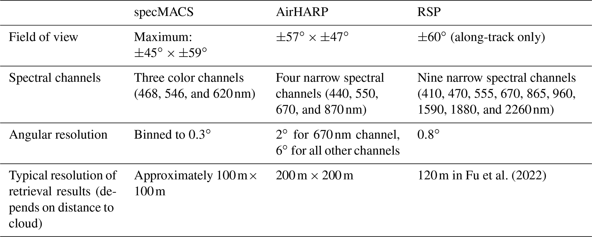
The major advantage of the specMACS and AirHARP instruments is their imaging capability with a large field of view. This not only increases the information content of the data but also makes it easier to measure the cloudbow because the cloudbow is observed within the field of view of the cameras for a large range of solar zenith angles. specMACS enables an even more detailed representation of the spatial distribution of the DSD, due to the higher spatial resolution (100 m) compared with AirHARP (200 m). RSP has the highest number of spectral channels (nine), including SWIR channels and can, therefore, simultaneously retrieve the reff based on the bispectral technique without any alignment errors. specMACS also offers the possibility for a bispectral retrieval because of its additional two spectrometers, but these have a smaller field of view compared with the polarization cameras. Furthermore, RSP and AirHARP have narrower spectral channels compared with specMACS, which sharpens the cloudbow signal and improves the sensitivity of the retrieval, especially for large droplets. However, the specMACS measurements have the highest angular resolution. From a technical perspective, it is interesting that a high angular resolution is required to retrieve such large reff, as retrieved in case study 1, because the cloudbow signal becomes narrower for large reff (see Fig. 5a). To determine the required angular resolution, Miller et al. (2018) used the Nyquist frequency, which defines the minimum sampling resolution needed to resolve features of an oscillating signal. In addition to the reff, the required angular resolution depends on the wavelength λ, with shorter wavelengths requiring a higher angular resolution (shown, e.g., in Fig. 1a in McBride et al., 2020). The Nyquist resolution for λ=670 nm and reff=40 µm is approximately 1.5∘ according to Miller et al. (2018). This is a challenge for some polarimetric instruments because they do not measure with the necessary angular resolution; for example, POLDER measures from 4 to 10∘ (Shang et al., 2015) and AirHARP measures at 2∘ (McBride et al., 2020). RSP measures at an angular resolution of 0.8∘ and does retrieve reff larger than 30 µm; however, an example of such large reff has not yet been discussed in any study, as mentioned in Sinclair et al. (2021). The need for a high angular resolution is no limitation for the specMACS instrument (measurements are binned onto a grid with a step size 0.3∘).
As mentioned above, the large field of view of the specMACS instrument favors the observation of the cloudbow. We assessed how often the cloudbow retrieval can actually be applied under typical observation conditions. Only measurements that cover the whole scattering angle range of 135 to 165∘ are evaluated (see evaluable stripes in Figs. 7 and 12). Although we need this special observation geometry, the acquired cloudbow dataset is very large. During daytime under optimal cloudbow conditions (high solar zenith angle), approximately 45 % of the field of view of one camera can be analyzed, corresponding to an 8 km wide swath at a 10 km flight altitude. We computed the area of the evaluable stripe averaged over all EUREC4A measurements (130 flight hours) including night flights. The analysis showed that, on average, when combining the measurements of the two cameras, a stripe consisting of 25 % of all pixels of an image can be evaluated. It should be noted that several EUREC4A HALO flights were partly conducted during nighttime (Konow et al., 2021), when the observation of the cloudbow is, of course, impossible. A recent study by Thompson et al. (2022) evaluated the sampled scattering angle range of multiangle satellite instruments depending on different factors, such as the solar and view geometry or the location, season, and swath width, in more detail.
A statistical evaluation of all EUREC4A flights, with special attention paid to the differences in cloud microphysics for the different mesoscale patterns of trade-wind clouds (sugar, gravel, fish, and flower), is planned. Further processing steps will include comparisons of the polarimetric retrieval with bispectral retrievals from both specMACS and satellites, such as MODIS and GOES, as well as validation of the polarimetric retrieval with in situ measurements. During EUREC4A, the British research aircraft Twin Otter and the French aircraft ATR 42 collected measurements inside the clouds; these measurements will be compared to our results. Further validation is planned with in situ data from the recent CIRRUS-HL (2021) and HALO-(AC)3 (2022) campaigns. Moreover, we plan to apply the RFT technique (Alexandrov et al., 2012b) to specMACS measurements in the future, which will be particularly interesting for case studies involving bimodal DSDs. In addition, the retrieval will also be applied to the spatially limited but very precise measurements of the backscatter glory.
specMACS offers great potential for further evaluations of clouds. In future, the measurements of the different specMACS cameras (polarimetric and hyperspectral) will be combined to retrieve information about the variation in cloud microphysical properties with height inside the cloud and to identify the thermodynamic phase of the observed clouds. Furthermore, the HALO remote sensing payload makes it possible to deepen the understanding of clouds by combining the measurements of the different instruments.
The specMACS data used in this study are available upon request from the corresponding author. The WALES data used in this study are available from the EUREC4A database of AERIS (https://doi.org/10.25326/216, Wirth, 2021). The HAMP radar data used in this study are available upon request from the instrument PIs Lutz Hirsch (lutz.hirsch@mpimet.mpg.de) and Felix Ament (felix.ament@uni-hamburg.de).
TK, TZ, BM, LF, and VP actively participated in the EUREC4A field campaign. TK, TZ, and BM prepared the field campaign and provided valuable input during the development of the method. TK designed the data file format, developed the stereo method, and provided software for initial use. LV improved the stereo method and applied it to the data of the EUREC4A field campaign. AW carried out the geometric calibration of the cameras and provided the software code to process and calibrate the raw data. CE provided valuable input about polarization. BM and CE helped carry out the phase matrix simulations. VP developed the polarimetric cloudbow algorithm, processed and visualized the data, and wrote the manuscript with input from all co-authors.
At least one of the (co-)authors is a member of the editorial board of Atmospheric Measurement Techniques. The peer-review process was guided by an independent editor, and the authors also have no other competing interests to declare.
Publisher’s note: Copernicus Publications remains neutral with regard to jurisdictional claims in published maps and institutional affiliations.
We wish to thank the EUREC4A project team for collaboration and support; special thanks go to the DLR flight operations team for planning and executing the HALO flights. Furthermore, we wish to acknowledge Andreas Giez, Vladyslav Nenakhov, Martin Zöger, and Christian Mallaun for providing the BAHAMAS dataset and valuable information about it; Silke Groß and Martin Wirth for providing the WALES lidar data; Alexander Scheiderer and Zhoutong Ma for developing the cloud mask algorithm; and Heike Konow and Lutz Hirsch for sharing the HAMP radar data and for providing valuable information about the data. The data used in this publication were gathered during the EUREC4A field campaign and are made available via the Meteorologisches Institut, Ludwig-Maximilians-Universität München.
This research has been supported by Bjorn Stevens (Max Planck Institute for Meteorology Hamburg) and Markus Rapp (Institute of Atmospheric Physics, DLR Oberpfaffenhofen), the European Research Council (ERC), the Max Planck Society (MPG), the German Research Foundation (DFG, project SPP 1294), the German Meteorological Weather Service (DWD), and the German Aerospace Center (DLR).
This paper was edited by Wiebke Frey and reviewed by Bastiaan van Diedenhoven and one anonymous referee.
Albrecht, B. A.: Aerosols, Cloud Microphysics, and Fractional Cloudiness, Science, 245, 1227–1230, https://doi.org/10.1126/science.245.4923.1227, 1989. a
Alexandrov, M. D., Cairns, B., Emde, C., Ackerman, A. S., and van Diedenhoven, B.: Accuracy assessments of cloud droplet size retrievals from polarized reflectance measurements by the research scanning polarimeter, Remote Sens. Environ., 125, 92–111, https://doi.org/10.1016/j.rse.2012.07.012, 2012a. a, b, c, d, e, f, g, h, i, j
Alexandrov, M. D., Cairns, B., and Mishchenko, M. I.: Rainbow Fourier transform, J. Quant. Spectrosc. Ra., 113, 2521–2535, https://doi.org/10.1016/j.jqsrt.2012.03.025, 2012b. a, b, c, d
Alexandrov, M. D., Cairns, B., Wasilewski, A. P., Ackerman, A. S., McGill, M. J., Yorks, J. E., Hlavka, D. L., Platnick, S. E., Thomas Arnold, G., van Diedenhoven, B., Chowdhary, J., Ottaviani, M., and Knobelspiesse, K. D.: Liquid water cloud properties during the Polarimeter Definition Experiment (PODEX), Remote Sens. Environ., 169, 20–36, https://doi.org/10.1016/j.rse.2015.07.029, 2015. a, b, c, d
Alexandrov, M. D., Cairns, B., van Diedenhoven, B., Ackerman, A. S., Wasilewski, A. P., McGill, M. J., Yorks, J. E., Hlavka, D. L., Platnick, S. E., and Arnold, G. T.: Polarized view of supercooled liquid water clouds, Remote Sens. Environ., 181, 96–110, https://doi.org/10.1016/j.rse.2016.04.002, 2016. a
Alexandrov, M. D., Cairns, B., Sinclair, K., Wasilewski, A. P., Ziemba, L., Crosbie, E., Moore, R., Hair, J., Scarino, A. J., Hu, Y., Stamnes, S., Shook, M. A., and Chen, G.: Retrievals of cloud droplet size from the research scanning polarimeter data: Validation using in situ measurements, Remote Sens. Environ., 210, 76–95, https://doi.org/10.1016/j.rse.2018.03.005, 2018. a
Bass, M., Stryland, E. W. V., Williams, D. R., and Wolfe, W. L.: Handbook of Optics Volume II Devices, Measurements, and Properties 2nd edition, Handbook of Optics Volume II Devices, McGraw Hill LLC, ISBN 0-07-047974-7, 1995. a, b
Bony, S. and Dufresne, J.-L.: Marine boundary layer clouds at the heart of tropical cloud feedback uncertainties in climate models, Geophys. Res. Lett., 32, L20806, https://doi.org/10.1029/2005GL023851, 2005. a
Bony, S., Stevens, B., Ament, F., Bigorre, S., Chazette, P., Crewell, S., Delanoë, J., Emanuel, K., Farrell, D., Flamant, C., Gross, S., Hirsch, L., Karstensen, J., Mayer, B., Nuijens, L., Ruppert, J. H., Sandu, I., Siebesma, P., Speich, S., Szczap, F., Totems, J., Vogel, R., Wendisch, M., and Wirth, M.: EUREC4A: A Field Campaign to Elucidate the Couplings Between Clouds, Convection and Circulation, Surveys in Geophysics, 38, 1529–1568, https://doi.org/10.1007/s10712-017-9428-0, 2017. a
Bony, S., Schulz, H., Vial, J., and Stevens, B.: Sugar, Gravel, Fish, and Flowers: Dependence of Mesoscale Patterns of Trade-Wind Clouds on Environmental Conditions, Geophys. Res. Lett., 47, e2019GL085988, https://doi.org/10.1029/2019GL085988, 2020. a
Bradski, G.: The OpenCV Library, Dr. Dobb's Journal of Software Tools, https://github.com/opencv/opencv (last access: 2 February 2023), 2000. a
Brenguier, J.-L. and Chaumat, L.: Droplet Spectra Broadening in Cumulus Clouds. Part I: Broadening in Adiabatic Cores, J. Atmos. Sci., 58, 628–641, https://doi.org/10.1175/1520-0469(2001)058<0628:DSBICC>2.0.CO;2, 2001. a
Bréon, F.-M. and Doutriaux-Boucher, M.: A comparison of cloud droplet radii measured from space, IEEE T. Geosci. Remote, 43, 1796–1805, 2005. a, b, c, d
Bréon, F.-M. and Goloub, P.: Cloud droplet effective radius from spaceborne polarization measurements, Geophys. Res. Lett., 25, 1879–1882, 1998. a, b, c, d, e, f, g
Cairns, B., Russell, E. E., and Travis, L. D.: The Research Scanning Polarimeter: Calibration and ground-based measurements, in: Polarization: Measurement, Analysis, and Remote Sensing II, 18 Jul. 1999, Denver, Col., vol. 3754 of Proc. SPIE, p. 186, https://doi.org/10.1117/12.366329, 1999. a
Dauhut, T., Couvreux, F., Bouniol, D., Beucher, F., Volkmer, L., Pörtge, V., Schäfer, M., Ayet, A., Brilouet, P.-E., Jacob, M., and Wirth, M.: Flower trade-wind clouds are shallow mesoscale convective systems, Q. J. Roy. Meteorol. Soc., https://doi.org/10.1002/qj.4409, online first, 2022. a
Di Noia, A., Hasekamp, O. P., van Diedenhoven, B., and Zhang, Z.: Retrieval of liquid water cloud properties from POLDER-3 measurements using a neural network ensemble approach, Atmos. Meas. Tech., 12, 1697–1716, https://doi.org/10.5194/amt-12-1697-2019, 2019. a
Diner, D. J., Xu, F., Garay, M. J., Martonchik, J. V., Rheingans, B. E., Geier, S., Davis, A., Hancock, B. R., Jovanovic, V. M., Bull, M. A., Capraro, K., Chipman, R. A., and McClain, S. C.: The Airborne Multiangle SpectroPolarimetric Imager (AirMSPI): a new tool for aerosol and cloud remote sensing, Atmos. Meas. Tech., 6, 2007–2025, https://doi.org/10.5194/amt-6-2007-2013, 2013. a, b
Diner, D. J., Boland, S. W., Brauer, M., Bruegge, C., Burke, K. A., Chipman, R., Girolamo, L. D., Garay, M. J., Hasheminassab, S., Hyer, E., Jerrett, M., Jovanovic, V., Kalashnikova, O. V., Liu, Y., Lyapustin, A. I., Martin, R. V., Nastan, A., Ostro, B. D., Ritz, B., Schwartz, J., Wang, J., and Xu, F.: Advances in multiangle satellite remote sensing of speciated airborne particulate matter and association with adverse health effects: from MISR to MAIA, J. Appl. Remote Sens., 12, 042603, https://doi.org/10.1117/1.JRS.12.042603, 2018. a
Dubovik, O., Li, Z., Mishchenko, M. I., Tanré, D., Karol, Y., Bojkov, B., Cairns, B., Diner, D. J., Espinosa, W. R., Goloub, P., Gu, X., Hasekamp, O., Hong, J., Hou, W., Knobelspiesse, K. D., Landgraf, J., Li, L., Litvinov, P., Liu, Y., Lopatin, A., Marbach, T., Maring, H., Martins, V., Meijer, Y., Milinevsky, G., Mukai, S., Parol, F., Qiao, Y., Remer, L., Rietjens, J., Sano, I., Stammes, P., Stamnes, S., Sun, X., Tabary, P., Travis, L. D., Waquet, F., Xu, F., Yan, C., and Yin, D.: Polarimetric remote sensing of atmospheric aerosols: Instruments, methodologies, results, and perspectives, J. Quant. Spectrosc. Ra., 224, 474–511, https://doi.org/10.1016/j.jqsrt.2018.11.024, 2019. a
Emde, C., Buras, R., Mayer, B., and Blumthaler, M.: The impact of aerosols on polarized sky radiance: model development, validation, and applications, Atmos. Chem. Phys., 10, 383–396, https://doi.org/10.5194/acp-10-383-2010, 2010. a, b
Emde, C., Barlakas, V., Cornet, C., Evans, F., Korkin, S., Ota, Y., Labonnote, L. C., Lyapustin, A., Macke, A., Mayer, B., and Wendisch, M.: IPRT polarized radiative transfer model intercomparison project – Phase A, J. Quant. Spectrosc. Ra., 164, 8–36, https://doi.org/10.1016/j.jqsrt.2015.05.007, 2015. a
Emde, C., Buras-Schnell, R., Kylling, A., Mayer, B., Gasteiger, J., Hamann, U., Kylling, J., Richter, B., Pause, C., Dowling, T., and Bugliaro, L.: The libRadtran software package for radiative transfer calculations (version 2.0.1), Geosci. Model Dev., 9, 1647–1672, https://doi.org/10.5194/gmd-9-1647-2016, 2016. a
Eshelman, L. M. and Shaw, J. A.: Visualization of all-sky polarization images referenced in the instrument, scattering, and solar principal planes, Optical Engineering, 58, 082418, https://doi.org/10.1117/1.OE.58.8.082418, 2019. a, b
Ewald, F., Kölling, T., Baumgartner, A., Zinner, T., and Mayer, B.: Design and characterization of specMACS, a multipurpose hyperspectral cloud and sky imager, Atmos. Meas. Tech., 9, 2015–2042, https://doi.org/10.5194/amt-9-2015-2016, 2016. a, b, c, d
Ewald, F., Zinner, T., Kölling, T., and Mayer, B.: Remote sensing of cloud droplet radius profiles using solar reflectance from cloud sides – Part 1: Retrieval development and characterization, Atmos. Meas. Tech., 12, 1183–1206, https://doi.org/10.5194/amt-12-1183-2019, 2019. a, b
Forster, P., Storelvmo, T., Armour, K., Collins, W., Dufresne, J.-L., Frame, D., Lunt, D., Mauritsen, T., Palmer, M., Watanabe, M., Wild, M., and Zhang, H.: The Earth’s Energy Budget, Climate Feedbacks, and Climate Sensitivity, 923–1054, Cambridge University Press, Cambridge, United Kingdom and New York, NY, USA, https://www.ipcc.ch/report/ar6/wg1/downloads/report/IPCC_AR6_WGI_Chapter07.pdf (last access: 2 February 2023), 2021. a
Fougnie, B., Marbach, T., Lacan, A., Lang, R., Schlüssel, P., Poli, G., Munro, R., and Couto, A. B.: The multi-viewing multi-channel multi-polarisation imager – Overview of the 3MI polarimetric mission for aerosol and cloud characterization, J. Quant. Spectrosc. Ra., 219, 23–32, https://doi.org/10.1016/j.jqsrt.2018.07.008, 2018. a
Fu, D., Di Girolamo, L., Liang, L., and Zhao, G.: Regional Biases in MODIS Marine Liquid Water Cloud Drop Effective Radius Deduced Through Fusion With MISR, J. Geophys. Res.-Atmos., 124, 13182–13196, https://doi.org/10.1029/2019JD031063, 2019. a
Fu, D., Di Girolamo, L., Rauber, R. M., McFarquhar, G. M., Nesbitt, S. W., Loveridge, J., Hong, Y., van Diedenhoven, B., Cairns, B., Alexandrov, M. D., Lawson, P., Woods, S., Tanelli, S., Schmidt, S., Hostetler, C., and Scarino, A. J.: An evaluation of the liquid cloud droplet effective radius derived from MODIS, airborne remote sensing, and in situ measurements from CAMP2Ex, Atmos. Chem. Phys., 22, 8259–8285, https://doi.org/10.5194/acp-22-8259-2022, 2022. a, b
Giez, A., Mallaun, C., Nenakhov, V., and Zöger, M.: Calibration of a Nose Boom Mounted Airflow Sensor on an Atmospheric Research Aircraft by Inflight Maneuvers, DLR-Forschungsbericht, DLR-FB-2021-17, https://elib.dlr.de/145969/ (last access: 31 January 2023), 2021. a, b
Grabowski, W. W. and Wang, L.-P.: Growth of Cloud Droplets in a Turbulent Environment, Annu. Rev. Fluid Mech., 45, 293–324, https://doi.org/10.1146/annurev-fluid-011212-140750, 2013. a
Hansen, J. E.: Multiple scattering of polarized light in planetary atmospheres part II. Sunlight reflected by terrestrial water clouds, J. Atmos. Sci., 28, 1400–1426, 1971. a, b, c, d, e, f
Hansen, J. E. and Travis, L. D.: Light scattering in planetary atmospheres, Space Sci. Rev., 16, 527–610, https://doi.org/10.1007/BF00168069, 1974. a, b, c, d
Hasekamp, O. P.: Capability of multi-viewing-angle photo-polarimetric measurements for the simultaneous retrieval of aerosol and cloud properties, Atmos. Meas. Tech., 3, 839–851, https://doi.org/10.5194/amt-3-839-2010, 2010. a
Hasekamp, O. P. and Landgraf, J.: Retrieval of aerosol properties over land surfaces: capabilities of multiple-viewing-angle intensity and polarization measurements, Appl. Opt., 46, 3332–3344, https://doi.org/10.1364/AO.46.003332, 2007. a
Hersbach, H., Bell, B., Berrisford, P., Biavati, G., Horányi, A., Muñoz Sabater, J., Nicolas, J., Peubey, C., Radu, R., Rozum, I., Schepers, D., Simmons, A., Soci, C., Dee, D., and Thépaut, J.-N.: ERA5 hourly data on pressure levels from 1959 to present., Copernicus climate change service (c3s) climate data store (cds), https://doi.org/10.24381/cds.bd0915c6, 2018. a
Hersbach, H., Bell, B., Berrisford, P., Hirahara, S., Horányi, A., Muñoz-Sabater, J., Nicolas, J., Peubey, C., Radu, R., Schepers, D., Simmons, A., Soci, C., Abdalla, S., Abellan, X., Balsamo, G., Bechtold, P., Biavati, G., Bidlot, J., Bonavita, M., De Chiara, G., Dahlgren, P., Dee, D., Diamantakis, M., Dragani, R., Flemming, J., Forbes, R., Fuentes, M., Geer, A., Haimberger, L., Healy, S., Hogan, R. J., Hólm, E., Janisková, M., Keeley, S., Laloyaux, P., Lopez, P., Lupu, C., Radnoti, G., de Rosnay, P., Rozum, I., Vamborg, F., Villaume, S., and Thépaut, J.-N.: The ERA5 global reanalysis, Q. J. Roy. Meteorol. Soc., 146, 1999–2049, 2020. a
IPCC: Annex VII: Glossary, edited by: Matthews, J. B. R., Möller, V., van Diemen, R., Fuglestvedt, J. S., Masson-Delmotte, V., Méndez, C., Semenov, S., and Reisinger, A., Cambridge University Press, Cambridge, United Kingdom and New York, NY, USA, 2215–2256, https://www.ipcc.ch/report/ar6/wg1/downloads/report/IPCC_AR6_WGI_AnnexVII.pdf (last access: 2 February 2023), 2021. a
Knobelspiesse, K., Cairns, B., Redemann, J., Bergstrom, R. W., and Stohl, A.: Simultaneous retrieval of aerosol and cloud properties during the MILAGRO field campaign, Atmos. Chem. Phys., 11, 6245–6263, https://doi.org/10.5194/acp-11-6245-2011, 2011. a
Knobelspiesse, K., Tan, Q., Bruegge, C., Cairns, B., Chowdhary, J., van Diedenhoven, B., Diner, D., Ferrare, R., van Harten, G., Jovanovic, V., Ottaviani, M., Redemann, J., Seidel, F., and Sinclair, K.: Intercomparison of airborne multi-angle polarimeter observations from the Polarimeter Definition Experiment, Appl. Opt., 58, 650–669, https://doi.org/10.1364/AO.58.000650, 2019. a
Kölling, T., Zinner, T., and Mayer, B.: Aircraft-based stereographic reconstruction of 3-D cloud geometry, Atmos. Meas. Tech., 12, 1155–1166, https://doi.org/10.5194/amt-12-1155-2019, 2019. a, b, c, d, e, f
Konow, H., Ewald, F., George, G., Jacob, M., Klingebiel, M., Kölling, T., Luebke, A. E., Mieslinger, T., Pörtge, V., Radtke, J., Schäfer, M., Schulz, H., Vogel, R., Wirth, M., Bony, S., Crewell, S., Ehrlich, A., Forster, L., Giez, A., Gödde, F., Groß, S., Gutleben, M., Hagen, M., Hirsch, L., Jansen, F., Lang, T., Mayer, B., Mech, M., Prange, M., Schnitt, S., Vial, J., Walbröl, A., Wendisch, M., Wolf, K., Zinner, T., Zöger, M., Ament, F., and Stevens, B.: EUREC4A's HALO, Earth Syst. Sci. Data, 13, 5545–5563, https://doi.org/10.5194/essd-13-5545-2021, 2021. a, b, c, d
Krautstrunk, M. and Giez, A.: The Transition From FALCON to HALO Era Airborne Atmospheric Research, pp. 609–624, Springer Berlin Heidelberg, Berlin, Heidelberg, https://doi.org/10.1007/978-3-642-30183-4_37, 2012. a
LUCID Vision Labs Inc.: Phoenix 5.0 MP Polarized Tech Ref (PHX050S1-Q, Color, IMX264MYR), https://thinklucid.com/downloads-hub/#tab-phoenix-tech-man (last access: 23 August 2022), 2022a. a
LUCID Vision Labs Inc.: Phoenix 5.0 MP Polarization Model (IMX250MZR/MYR), https://thinklucid.com/de/product/phoenix-5-0-mp-polarized-model/ (last access: 23 August 2022), 2022b. a
Marshak, A., Platnick, S., Várnai, T., Wen, G., and Cahalan, R. F.: Impact of three-dimensional radiative effects on satellite retrievals of cloud droplet sizes, J. Geophys. Res.-Atmos., 111, D09207, https://doi.org/10.1029/2005JD006686, 2006. a, b
Martins, J. V., Fernandez-Borda, R., McBride, B., Remer, L., and Barbosa, H. M.: The harp hype ran gular imaging polarimeter and the need for small satellite payloads with high science payoff for earth science remote sensing, in: IGARSS 2018–2018 IEEE International Geoscience and Remote Sensing Symposium, 22–27 July 2018, Valencia, Spain, IEEE, 6304–6307, https://doi.org/10.1109/IGARSS.2018.8518823, 2018. a
Mayer, B. and Kylling, A.: Technical note: The libRadtran software package for radiative transfer calculations – description and examples of use, Atmos. Chem. Phys., 5, 1855–1877, https://doi.org/10.5194/acp-5-1855-2005, 2005. a
Mayer, B., Schröder, M., Preusker, R., and Schüller, L.: Remote sensing of water cloud droplet size distributions using the backscatter glory: a case study, Atmos. Chem. Phys., 4, 1255–1263, https://doi.org/10.5194/acp-4-1255-2004, 2004. a, b
McBride, B. A., Martins, J. V., Barbosa, H. M. J., Birmingham, W., and Remer, L. A.: Spatial distribution of cloud droplet size properties from Airborne Hyper-Angular Rainbow Polarimeter (AirHARP) measurements, Atmos. Meas. Tech., 13, 1777–1796, https://doi.org/10.5194/amt-13-1777-2020, 2020. a, b, c, d, e, f, g, h, i, j, k, l
Mech, M., Orlandi, E., Crewell, S., Ament, F., Hirsch, L., Hagen, M., Peters, G., and Stevens, B.: HAMP – the microwave package on the High Altitude and LOng range research aircraft (HALO), Atmos. Meas. Tech., 7, 4539–4553, https://doi.org/10.5194/amt-7-4539-2014, 2014. a
Mie, G.: Beiträge zur Optik trüber Medien, speziell kolloidaler Metallösungen, Ann. Phys., 330, 377–445, https://doi.org/10.1002/andp.19083300302, 1908. a
Miles, N. L., Verlinde, J., and Clothiaux, E. E.: Cloud Droplet Size Distributions in Low-Level Stratiform Clouds, J. Atmos. Sci., 57, 295–311, https://doi.org/10.1175/1520-0469(2000)057<0295:CDSDIL>2.0.CO;2, 2000. a
Miller, D. J., Zhang, Z., Platnick, S., Ackerman, A. S., Werner, F., Cornet, C., and Knobelspiesse, K.: Comparisons of bispectral and polarimetric retrievals of marine boundary layer cloud microphysics: case studies using a LES–satellite retrieval simulator, Atmos. Meas. Tech., 11, 3689–3715, https://doi.org/10.5194/amt-11-3689-2018, 2018. a, b
Mishchenko, M. I. and Travis, L. D.: Satellite retrieval of aerosol properties over the ocean using measurements of reflected sunlight: Effect of instrumental errors and aerosol absorption, J. Geophys. Res.-Atmos., 102, 13543–13553, https://doi.org/10.1029/97JD01124, 1997. a
Nakajima, T. and King, M. D.: Determination of the Optical Thickness and Effective Particle Radius of Clouds from Reflected Solar Radiation Measurements. Part I: Theory, J. Atmos. Sci. 47, 1878–1893, https://doi.org/10.1175/1520-0469(1990)047<1878:DOTOTA>2.0.CO;2, 1990. a, b
Otsu, N.: A Threshold Selection Method from Gray-Level Histograms, IEEE Transactions on Systems, Man, and Cybernetics, 9, 62–66, https://doi.org/10.1109/TSMC.1979.4310076, 1979. a
Painemal, D., Spangenberg, D., Smith Jr., W. L., Minnis, P., Cairns, B., Moore, R. H., Crosbie, E., Robinson, C., Thornhill, K. L., Winstead, E. L., and Ziemba, L.: Evaluation of satellite retrievals of liquid clouds from the GOES-13 imager and MODIS over the midlatitude North Atlantic during the NAAMES campaign, Atmos. Meas. Tech., 14, 6633–6646, https://doi.org/10.5194/amt-14-6633-2021, 2021. a
Pinsky, M., Khain, A., and Korolev, A.: Theoretical analysis of mixing in liquid clouds – Part 3: Inhomogeneous mixing, Atmos. Chem. Phys., 16, 9273–9297, https://doi.org/10.5194/acp-16-9273-2016, 2016. a
Platnick, S.: Vertical photon transport in cloud remote sensing problems, J. Geophys. Res.-Atmos., 105, 22919–22935, https://doi.org/10.1029/2000JD900333, 2000. a
Platnick, S., King, M., Ackerman, S., Menzel, W., Baum, B., Riedi, J., and Frey, R.: The MODIS cloud products: algorithms and examples from Terra, IEEE T. Geosci. Remote, 41, 459–473, https://doi.org/10.1109/TGRS.2002.808301, 2003. a
Platnick, S., Meyer, K. G., King, M. D., Wind, G., Amarasinghe, N., Marchant, B., Arnold, G. T., Zhang, Z., Hubanks, P. A., Holz, R. E., Yang, P., Ridgway, W. L., and Riedi, J.: The MODIS Cloud Optical and Microphysical Products: Collection 6 Updates and Examples From Terra and Aqua, IEEE T. Geosci. Remote, 55, 502–525, https://doi.org/10.1109/TGRS.2016.2610522, 2017. a
Polonik, P., Knote, C., Zinner, T., Ewald, F., Kölling, T., Mayer, B., Andreae, M. O., Jurkat-Witschas, T., Klimach, T., Mahnke, C., Molleker, S., Pöhlker, C., Pöhlker, M. L., Pöschl, U., Rosenfeld, D., Voigt, C., Weigel, R., and Wendisch, M.: The challenge of simulating the sensitivity of the Amazonian cloud microstructure to cloud condensation nuclei number concentrations, Atmos. Chem. Phys., 20, 1591–1605, https://doi.org/10.5194/acp-20-1591-2020, 2020. a
Remer, L. A., Knobelspiesse, K., Zhai, P.-W., Xu, F., Kalashnikova, O. V., Chowdhary, J., Hasekamp, O., Dubovik, O., Wu, L., Ahmad, Z., Boss, E., Cairns, B., Coddington, O., Davis, A. B., Dierssen, H. M., Diner, D. J., Franz, B., Frouin, R., Gao, B.-C., Ibrahim, A., Levy, R. C., Martins, J. V., Omar, A. H., and Torres, O.: Retrieving Aerosol Characteristics From the PACE Mission, Part 2: Multi-Angle and Polarimetry, Front. Environ. Sci., 7, 94, https://doi.org/10.3389/fenvs.2019.00094, 2019. a, b, c
Riedi, J., Marchant, B., Platnick, S., Baum, B. A., Thieuleux, F., Oudard, C., Parol, F., Nicolas, J.-M., and Dubuisson, P.: Cloud thermodynamic phase inferred from merged POLDER and MODIS data, Atmos. Chem. Phys., 10, 11851–11865, https://doi.org/10.5194/acp-10-11851-2010, 2010. a
Rosenfeld, D. and Lensky, I. M.: Satellite-Based Insights into Precipitation Formation Processes in Continental and Maritime Convective Clouds, B. Am. Meteorol. Soc., 79, 2457–2476, https://doi.org/10.1175/1520-0477(1998)079<2457:SBIIPF>2.0.CO;2, 1998. a, b
Satoh, M., Stevens, B., Judt, F., Khairoutdinov, M., Lin, S.-J., Putman, W. M., and Düben, P.: Global Cloud-Resolving Models, Current Climate Change Reports, 5, 172–184, https://doi.org/10.1007/s40641-019-00131-0, 2019. a
Schulz, H., Eastman, R., and Stevens, B.: Characterization and Evolution of Organized Shallow Convection in the Downstream North Atlantic Trades, J. Geophys. Res.-Atmos., 126, e2021JD034575, https://doi.org/10.1029/2021JD034575, 2021. a
Shang, H., Chen, L., Bréon, F. M., Letu, H., Li, S., Wang, Z., and Su, L.: Impact of cloud horizontal inhomogeneity and directional sampling on the retrieval of cloud droplet size by the POLDER instrument, Atmos. Meas. Tech., 8, 4931–4945, https://doi.org/10.5194/amt-8-4931-2015, 2015. a, b
Shang, H., Letu, H., Bréon, F.-M., Riedi, J., Ma, R., Wang, Z., Nakajima, T. Y., Wang, Z., and Chen, L.: An improved algorithm of cloud droplet size distribution from POLDER polarized measurements, Remote Sens. Environ., 228, 61–74, https://doi.org/10.1016/j.rse.2019.04.013, 2019. a
Sinclair, K., van Diedenhoven, B., Cairns, B., Alexandrov, M., Dzambo, A. M., and L'Ecuyer, T.: Inference of Precipitation in Warm Stratiform Clouds Using Remotely Sensed Observations of the Cloud Top Droplet Size Distribution, Geophys. Res. Lett., 48, e2021GL092547, https://doi.org/10.1029/2021GL092547, 2021. a, b
Spinhirne, J. D. and Nakajima, T.: Glory of clouds in the near infrared, Appl. Opt., 33, 4652–4662, https://doi.org/10.1364/AO.33.004652, 1994. a
Stap, F., Hasekamp, O., Emde, C., and Röckmann, T.: Influence of 3D effects on 1D aerosol retrievals in synthetic, partially clouded scenes, J. Quant. Spectrosc. Ra., 170, 54–68, https://doi.org/10.1016/j.jqsrt.2015.10.008, 2016a. a
Stap, F. A., Hasekamp, O. P., Emde, C., and Röckmann, T.: Multiangle photopolarimetric aerosol retrievals in the vicinity of clouds: Synthetic study based on a large eddy simulation, J. Geophys. Res.-Atmos., 121, 12914–12935, https://doi.org/10.1002/2016JD024787, 2016b. a
Sterzik, M. F., Bagnulo, S., Emde, C., and Manev, M.: The cloudbow of planet Earth observed in polarisation, A&A, 639, A89, https://doi.org/10.1051/0004-6361/202038270, 2020. a
Stevens, B., Ament, F., Bony, S., Crewell, S., Ewald, F., Gross, S., Hansen, A., Hirsch, L., Jacob, M., Kölling, T., Konow, H., Mayer, B., Wendisch, M., Wirth, M., Wolf, K., Bakan, S., Bauer-Pfundstein, M., Brueck, M., Delanoë, J., Ehrlich, A., Farrell, D., Forde, M., Gödde, F., Grob, H., Hagen, M., Jäkel, E., Jansen, F., Klepp, C., Klingebiel, M., Mech, M., Peters, G., Rapp, M., Wing, A. A., and Zinner, T.: A High-Altitude Long-Range Aircraft Configured as a Cloud Observatory: The NARVAL Expeditions, B. Am. Meteorol. Soc., 100, 1061–1077, https://doi.org/10.1175/BAMS-D-18-0198.1, 2019. a, b
Stevens, B., Bony, S., Brogniez, H., Hentgen, L., Hohenegger, C., Kiemle, C., L'Ecuyer, T. S., Naumann, A. K., Schulz, H., Siebesma, P. A., Vial, J., Winker, D. M., and Zuidema, P.: Sugar, gravel, fish and flowers: Mesoscale cloud patterns in the trade winds, Q. J. Roy. Meteorol. Soc., 146, 141–152, https://doi.org/10.1002/qj.3662, 2020. a, b
Stevens, B., Bony, S., Farrell, D., Ament, F., Blyth, A., Fairall, C., Karstensen, J., Quinn, P. K., Speich, S., Acquistapace, C., Aemisegger, F., Albright, A. L., Bellenger, H., Bodenschatz, E., Caesar, K.-A., Chewitt-Lucas, R., de Boer, G., Delanoë, J., Denby, L., Ewald, F., Fildier, B., Forde, M., George, G., Gross, S., Hagen, M., Hausold, A., Heywood, K. J., Hirsch, L., Jacob, M., Jansen, F., Kinne, S., Klocke, D., Kölling, T., Konow, H., Lothon, M., Mohr, W., Naumann, A. K., Nuijens, L., Olivier, L., Pincus, R., Pöhlker, M., Reverdin, G., Roberts, G., Schnitt, S., Schulz, H., Siebesma, A. P., Stephan, C. C., Sullivan, P., Touzé-Peiffer, L., Vial, J., Vogel, R., Zuidema, P., Alexander, N., Alves, L., Arixi, S., Asmath, H., Bagheri, G., Baier, K., Bailey, A., Baranowski, D., Baron, A., Barrau, S., Barrett, P. A., Batier, F., Behrendt, A., Bendinger, A., Beucher, F., Bigorre, S., Blades, E., Blossey, P., Bock, O., Böing, S., Bosser, P., Bourras, D., Bouruet-Aubertot, P., Bower, K., Branellec, P., Branger, H., Brennek, M., Brewer, A., Brilouet , P.-E., Brügmann, B., Buehler, S. A., Burke, E., Burton, R., Calmer, R., Canonici, J.-C., Carton, X., Cato Jr., G., Charles, J. A., Chazette, P., Chen, Y., Chilinski, M. T., Choularton, T., Chuang, P., Clarke, S., Coe, H., Cornet, C., Coutris, P., Couvreux, F., Crewell, S., Cronin, T., Cui, Z., Cuypers, Y., Daley, A., Damerell, G. M., Dauhut, T., Deneke, H., Desbios, J.-P., Dörner, S., Donner, S., Douet, V., Drushka, K., Dütsch, M., Ehrlich, A., Emanuel, K., Emmanouilidis, A., Etienne, J.-C., Etienne-Leblanc, S., Faure, G., Feingold, G., Ferrero, L., Fix, A., Flamant, C., Flatau, P. J., Foltz, G. R., Forster, L., Furtuna, I., Gadian, A., Galewsky, J., Gallagher, M., Gallimore, P., Gaston, C., Gentemann, C., Geyskens, N., Giez, A., Gollop, J., Gouirand, I., Gourbeyre, C., de Graaf, D., de Groot, G. E., Grosz, R., Güttler, J., Gutleben, M., Hall, K., Harris, G., Helfer, K. C., Henze, D., Herbert, C., Holanda, B., Ibanez-Landeta, A., Intrieri, J., Iyer, S., Julien, F., Kalesse, H., Kazil, J., Kellman, A., Kidane, A. T., Kirchner, U., Klingebiel, M., Körner, M., Kremper, L. A., Kretzschmar, J., Krüger, O., Kumala, W., Kurz, A., L'Hégaret, P., Labaste, M., Lachlan-Cope, T., Laing, A., Landschützer, P., Lang, T., Lange, D., Lange, I., Laplace, C., Lavik, G., Laxenaire, R., Le Bihan, C., Leandro, M., Lefevre, N., Lena, M., Lenschow, D., Li, Q., Lloyd, G., Los, S., Losi, N., Lovell, O., Luneau, C., Makuch, P., Malinowski, S., Manta, G., Marinou, E., Marsden, N., Masson, S., Maury, N., Mayer, B., Mayers-Als, M., Mazel, C., McGeary, W., McWilliams, J. C., Mech, M., Mehlmann, M., Meroni, A. N., Mieslinger, T., Minikin, A., Minnett, P., Möller, G., Morfa Avalos, Y., Muller, C., Musat, I., Napoli, A., Neuberger, A., Noisel, C., Noone, D., Nordsiek, F., Nowak, J. L., Oswald, L., Parker, D. J., Peck, C., Person, R., Philippi, M., Plueddemann, A., Pöhlker, C., Pörtge, V., Pöschl, U., Pologne, L., Posyniak, M., Prange, M., Quiñones Meléndez, E., Radtke, J., Ramage, K., Reimann, J., Renault, L., Reus, K., Reyes, A., Ribbe, J., Ringel, M., Ritschel, M., Rocha, C. B., Rochetin, N., Röttenbacher, J., Rollo, C., Royer, H., Sadoulet, P., Saffin, L., Sandiford, S., Sandu, I., Schäfer, M., Schemann, V., Schirmacher, I., Schlenczek, O., Schmidt, J., Schröder, M., Schwarzenboeck, A., Sealy, A., Senff, C. J., Serikov, I., Shohan, S., Siddle, E., Smirnov, A., Späth, F., Spooner, B., Stolla, M. K., Szkółka, W., de Szoeke, S. P., Tarot, S., Tetoni, E., Thompson, E., Thomson, J., Tomassini, L., Totems, J., Ubele, A. A., Villiger, L., von Arx, J., Wagner, T., Walther, A., Webber, B., Wendisch, M., Whitehall, S., Wiltshire, A., Wing, A. A., Wirth, M., Wiskandt, J., Wolf, K., Worbes, L., Wright, E., Wulfmeyer, V., Young, S., Zhang, C., Zhang, D., Ziemen, F., Zinner, T., and Zöger, M.: EUREC4A, Earth Syst. Sci. Data, 13, 4067–4119, https://doi.org/10.5194/essd-13-4067-2021, 2021. a
Thompson, S. N., van Diedenhoven, B., Colarco, P. R., Castellanos, P., Lian, E., and Martins, J. V.: Analysis of Scattering Angle Sampling by Multi-Angle Imaging Polarimeters for Different Orbit Geometries, Front. Remote Sens., 3, 836262, https://doi.org/10.3389/frsen.2022.836262, 2022. a
Twomey, S.: Pollution and the planetary albedo, Atmos. Environ. (1967), 8, 1251–1256, https://doi.org/10.1016/0004-6981(74)90004-3, 1974. a
Wagner, W. and Pruß, A.: The IAPWS formulation 1995 for the thermodynamic properties of ordinary water substance for general and scientific use, J. Phys. Chem. Ref. Data, 31, 387–535, 2002. a
Wendisch, M., Macke, A., Ehrlich, A., Lüpkes, C., Mech, M., Chechin, D., Dethloff, K., Velasco, C. B., Bozem, H., Brückner, M., Clemen, H.-C., Crewell, S., Donth, T., Dupuy, R., Ebell, K., Egerer, U., Engelmann, R., Engler, C., Eppers, O., Gehrmann, M., Gong, X., Gottschalk, M., Gourbeyre, C., Griesche, H., Hartmann, J., Hartmann, M., Heinold, B., Herber, A., Herrmann, H., Heygster, G., Hoor, P., Jafariserajehlou, S., Jäkel, E., Järvinen, E., Jourdan, O., Kästner, U., Kecorius, S., Knudsen, E. M., Köllner, F., Kretzschmar, J., Lelli, L., Leroy, D., Maturilli, M., Mei, L., Mertes, S., Mioche, G., Neuber, R., Nicolaus, M., Nomokonova, T., Notholt, J., Palm, M., van Pinxteren, M., Quaas, J., Richter, P., Ruiz-Donoso, E., Schäfer, M., Schmieder, K., Schnaiter, M., Schneider, J., Schwarzenböck, A., Seifert, P., Shupe, M. D., Siebert, H., Spreen, G., Stapf, J., Stratmann, F., Vogl, T., Welti, A., Wex, H., Wiedensohler, A., Zanatta, M., and Zeppenfeld, S.: The Arctic Cloud Puzzle: Using ACLOUD/PASCAL Multiplatform Observations to Unravel the Role of Clouds and Aerosol Particles in Arctic Amplification, B. Am. Meteorol. Soc., 100, 841–871, https://doi.org/10.1175/BAMS-D-18-0072.1, 2019. a
Wirth, M.: Cloud top height derived from airborne measurements with the WALES lidar during the EUREC4A field campaign, Aeris [data set], https://doi.org/10.25326/216, 2021. a, b
Wirth, M., Fix, A., Mahnke, P., Schwarzer, H., Schrandt, F., and Ehret, G.: The airborne multi-wavelength water vapor differential absorption lidar WALES: system design and performance, Appl. Phys. B, 96, 201, https://doi.org/10.1007/s00340-009-3365-7, 2009. a
Wiscombe, W. J.: Improved Mie scattering algorithms, Appl. Opt., 19, 1505–1509, https://doi.org/10.1364/AO.19.001505, 1980. a
Xu, F., van Harten, G., Diner, D. J., Davis, A. B., Seidel, F. C., Rheingans, B., Tosca, M., Alexandrov, M. D., Cairns, B., Ferrare, R. A., Burton, S. P., Fenn, M. A., Hostetler, C. A., Wood, R., and Redemann, J.: Coupled Retrieval of Liquid Water Cloud and Above-Cloud Aerosol Properties Using the Airborne Multiangle SpectroPolarimetric Imager (AirMSPI), J. Geophys. Res.-Atmos., 123, 3175–3204, https://doi.org/10.1002/2017JD027926, 2018. a
Zhang, Z.: A flexible new technique for camera calibration, IEEE Transactions on Pattern Analysis and Machine Intelligence, 22, 1330–1334, https://doi.org/10.1109/34.888718, 2000. a
Zhang, Z.: On the sensitivity of cloud effective radius retrieval based on spectral method to bi-modal droplet size distribution: A semi-analytical model, J. Quant. Spectrosc. Ra., 129, 79–88, https://doi.org/10.1016/j.jqsrt.2013.05.033, 2013. a
Zhang, Z., Ackerman, A. S., Feingold, G., Platnick, S., Pincus, R., and Xue, H.: Effects of cloud horizontal inhomogeneity and drizzle on remote sensing of cloud droplet effective radius: Case studies based on large-eddy simulations, J. Geophys. Res.-Atmos., 117, D19208, https://doi.org/10.1029/2012JD017655, 2012. a, b
Zinner, T., Marshak, A., Lang, S., Martins, J. V., and Mayer, B.: Remote sensing of cloud sides of deep convection: towards a three-dimensional retrieval of cloud particle size profiles, Atmos. Chem. Phys., 8, 4741–4757, https://doi.org/10.5194/acp-8-4741-2008, 2008. a
Zinner, T., Wind, G., Platnick, S., and Ackerman, A. S.: Testing remote sensing on artificial observations: impact of drizzle and 3-D cloud structure on effective radius retrievals, Atmos. Chem. Phys., 10, 9535–9549, https://doi.org/10.5194/acp-10-9535-2010, 2010. a
Zinner, T., Schwarz, U., Kölling, T., Ewald, F., Jäkel, E., Mayer, B., and Wendisch, M.: Cloud geometry from oxygen-A-band observations through an aircraft side window, Atmos. Meas. Tech., 12, 1167–1181, https://doi.org/10.5194/amt-12-1167-2019, 2019. a