New Absolute Cavity Pyrgeometer equation by application of Kirchhoff's law and adding a convection term

An equation for the Absolute Cavity Pyrgeometer (ACP) is derived from application of Kirchhoff's law and the addition of a convection term to account for the thermopile being open to the environment, unlike a domed radiometer. The equation is then used to investigate four methods to characterise key instrumental parameters using laboratory and field measurements. The first uses solar irradiance to estimate the thermopile responsivity, the second uses a minimisation method that solves for the thermopile responsivity and transmission of the cavity, and the third and fourth revisit the Reda et al. (2012) linear least squares calibration technique. Data were collected between January and November 2020, when the ACP96 and two IRIS radiometers monitoring terrestrial irradiances were available. The results indicate good agreement with IRIS irradiances using the new equation. The analysis also indicates that while the thermopile responsivity, concentrator transmission and emissivity of an ACP can be determined independently, as an open instrument, the impact of the convection term is minor in steady-state conditions but significant when the base of the instrument is being subjected to rapid artificial cooling or heating. Using laboratory characterisation of the transmission and emissivity, together with use of an estimated solar calibration of the thermopile, generated mean differences of less than 1.5 Wm⁻² to the two IRIS radiometers. A minimisation method using each IRIS radiometer as the reference also provided similar results, and the derived thermopile responsivity was within 0.3 µV W⁻¹ m² of the solar-calibration-derived infrared responsivity estimate of 10.5 µV W⁻¹ m² estimated using a nominal solar calibration and provide irradiances within ±2 % of the terrestrial irradiance measured by the reference pyrgeometers traceable to the International System of Units (SI). The calibration method using linear least squares regression introduced by Reda et al. (2012) that relies on rapid cooling of the ACP base but utilising the new equation was found to produce consistent results but was dependent on the assumed temperature of the air above the thermopile. This study demonstrates the potential of the ACP as another independent reference radiometer for terrestrial irradiance once the magnitude of the convection coefficient and any potential variations in it have been resolved.

1 Background

Reda et al. (2012) introduced the Absolute Cavity Pyrgeometer (ACP), its operational equations and its characterisation process. The ACP is an Eppley Laboratory Precision Infrared Radiometer (PIR) with its dome replaced by a symmetrical cavity (called the concentrator) internally coated by polished gold and a cooling and heating system attached to the base of the pyrgeometer to assist in cooling or heating the ACP body.

The Reda et al. (2012) derivation of the ACP equation uses a combination of radiative transfer but without consideration of reflected irradiance components and impacts of convection (Vignola et al., 2012). Blackbody calibration of an ACP has proven difficult, and Reda et al. (2012) proposed a method of characterisation and calibration that included laboratory methods to determine the transmission of the concentrator and the emissivity of polished gold, while the thermopile sensitivity is determined using a linear least squares regression (LSQ) technique in the field at night under stable incoming irradiance conditions. Calibrations provided by Reda et al. (2012) assumed that the responsivity and transmission of the ACP changes over hours and days with variations of the order of several percent. More recently, Gröbner (2021) showed that the selection of points used in the field calibration has a significant influence on the result.

The ACP's body uses an Eppley Laboratory F3 thermopile which is used for Eppley Laboratory pyranometers (PSPs) and pyrgeometers (PIRs). The stability of the F3 thermopile used for solar and infrared irradiance measurements in domed instruments is well within a percent over several years. Therefore, it was surprising to see the large variation in the ACP thermopile responsivity (µV (W⁻¹ m²)) reported by Reda et al. (2012).

This paper derives a new ACP equation that adheres to Kirchhoff's law of thermal radiation for radiative transfer in vacuum and in-air measurements with a thermopile not protected by a dome and therefore includes an energy transfer term due to convection. The similarity and key differences in the contributing terms of the new in-air and Reda et al. (2012) equations are also examined. Using the new equation, the impact on the laboratory characterisation, night-time calibration compared against two IRIS pyrgeometers, and an application of the linear LSQ methods are investigated.

2 The steady-state equation for an ACP without a dome or concentrator in a vacuum

An ACP without a concentrator is an Eppley Laboratory pyrgeometer without a dome that includes a thermistor to measure the temperature of the body. It has a flat thermopile receiver painted with Parsons Black. In a vacuum there is only radiative transfer between the source and the thermopile receiver, with no possibility of a convection component.

The ACP equation in this instance only involves Kirchhoff's law at the black surface of the thermopile receiver, namely

$$\begin{array}{}\text{(1)}& \mathrm{1}={\mathit{\alpha }}_{\mathrm{r}}+{\mathit{\rho }}_{\mathrm{r}},\end{array}$$

where α_r is the fraction absorbed by the receiver, which from Kirchhoff's law is equivalent to emissivity ε_r, and ρ_r is the fraction reflected from the receiver as there is no transmission through the black receiver surface.

The net flux between the incoming and outgoing flux results in a temperature difference between the base and receiver of the thermopile generating a voltage that is proportional to the net flux. That is,

$$\begin{array}{}\text{(2)}& \mathrm{KV}=F\downarrow -F\uparrow ,\end{array}$$

where K is the responsivity of the thermopile (Wm⁻² µV⁻¹), V is the voltage and F↓ and F↑ are the downward and upward radiant fluxes. The downward flux is made up of a single component of the irradiance from the source W:

$$\begin{array}{}\text{(3)}& F\downarrow =W.\end{array}$$

The upward flux has two components, the emission from the surface and the reflection of the incoming flux, that is,

$$\begin{array}{}\text{(4)}& F\uparrow ={\mathit{\epsilon }}_{\mathrm{r}}{W}_{\mathrm{r}}+\left(\mathrm{1}-{\mathit{\epsilon }}_{\mathrm{r}}\right)F\downarrow ,\end{array}$$

where ε_r is the emissivity of the receiver, and W_r is the blackbody irradiance from the receiver. ρ_r is equal to (1−ε_r) as there is no transmission through the receiver surface. Solving the two simultaneous equations, the result is

$$\begin{array}{}\text{(5)}& \mathrm{KV}=F\downarrow -F\uparrow =W{\mathit{\epsilon }}_{\mathrm{r}}-W_{\mathrm{r}}{\mathit{\epsilon }}_{\mathrm{r}}={\mathit{\epsilon }}_{\mathrm{r}}(W-W_{\mathrm{r}}),\end{array}$$

which gives, for W,

$$\begin{array}{}\text{(6)}& W={\displaystyle \frac{K}{{\mathit{\epsilon }}_{\mathrm{r}}}}\mathrm{V}+W_{\mathrm{r}}=K_{\mathrm{r}}\mathrm{V}+W_{\mathrm{r}},\end{array}$$

where K_r is the responsivity of the thermopile receiver or $K_{\mathrm{r}}=K/{\mathit{\epsilon }}_{\mathrm{r}}$.

W_r is given by $\mathit{\sigma }{T}_{\mathrm{r}}^{\mathrm{4}}$, where σ is the Stefan–Boltzmann constant and T_r is the temperature at the top of the receiver. As T_r cannot be measured directly at time t, it is approximated by

$$\begin{array}{}\text{(7)}& T_{\mathrm{r}}\left(t\right)=T_{\mathrm{b}}\left(t\right)+\mathrm{V}\left(t\right)S,\end{array}$$

where T_b is the ACP body temperature and S is calculated based on known values of the Seebeck coefficient for the thermopile junctions. If n is the number of junctions and ϖ is the efficiency of the thermopile, then

$$\begin{array}{}\text{(8)}& S={\displaystyle \frac{\mathrm{1}}{S_{\mathrm{0}}n\mathit{\varpi }}}.\end{array}$$

For the Eppley Laboratory F3 thermopile used in an ACP, with 56 copper–constantan junctions, S₀ is ∼40 µV K⁻¹, and Reda et al. (2012) suggested ϖ∼0.65 or 65 % efficiency. (T_r−T_b) is dependent on the net incoming irradiance and the thermal conductivity of the thermopile, while S is a property solely of the thermopile and impacts directly the thermopile responsivity. ϖ may vary due to the manufacturing process. During operation of an ACP, the maximum expected (T_r−T_b) is about 0.7 K. Reda et al. (2012) proposed S to be $\mathrm{7.044}\times {\mathrm{10}}^{-\mathrm{4}}$. For a T_b=273.15 K and steady-state conditions where $\mathrm{V}\sim -\mathrm{800}$ µV (corresponding to the net radiation exchange of the ACP with a cloud-free sky), if S is in error by 20 %, the impact on W_r is about 0.7 Wm⁻² and increases proportionally with V and T_b.

3 The steady-state equation of an ACP with a symmetrical concentrator in a vacuum

The concentrator is assumed to have symmetrical transmission, absorption and backscatter characteristics. That is,

$$\begin{array}{}\text{(9)}& \mathrm{1}=\mathit{\tau }+\mathit{\beta }+\mathit{\alpha },\end{array}$$

where τ is the transmitted fraction of the incoming irradiance through the concentrator, α is the fraction of the incoming irradiance absorbed by the concentrator and β is the fraction of the incoming irradiance reflected out of the concentrator. Being a symmetrical cavity, each component's magnitude will remain the same if irradiance enters either end of the concentrator.

The concentrator walls coated in gold have an emissivity (or absorptivity) of ε_c that is a property of the surface and is independent of the incoming irradiance. The fraction of incoming irradiance absorbed by the concentrator, α, is a consequence of ε_c and the multiple reflection of incoming irradiance on the concentrator walls, and hence α≥ε_c.

For an ACP in a vacuum, the incoming flux F↓ at the receiver (at one end of the symmetrical concentrator) has three components, the transmitted incoming atmospheric irradiance τW, any emission from the walls of the concentrator with a blackbody irradiance of W_c, ε_cW_c, and the back reflectance towards the receiver of the flux from the receiver βF↑, that is,

$$\begin{array}{}\text{(10)}& F\downarrow =\mathit{\tau }W+{\mathit{\epsilon }}_{\mathrm{c}}{W}_{\mathrm{c}}+\mathit{\beta }F\uparrow .\end{array}$$

The outgoing flux from the receiver is made up of two components in Eq. (4); thus,

$$\begin{array}{}\text{(11)}& F\downarrow ={\displaystyle \frac{\mathit{\tau }W+{\mathit{\epsilon }}_{\mathrm{c}}{W}_{\mathrm{c}}+\mathit{\beta }{\mathit{\epsilon }}_{\mathrm{r}}{W}_{\mathrm{r}}}{\mathrm{1}-\mathit{\beta }(\mathrm{1}-{\mathit{\epsilon }}_{\mathrm{r}})}}.\end{array}$$

Solving the two simultaneous equations results in

$$\begin{array}{}\text{(12)}& \mathrm{KV}=F\downarrow -F\uparrow ={\displaystyle \frac{{\mathit{\epsilon }}_{\mathrm{r}}(\mathit{\tau }W+{\mathit{\epsilon }}_{\mathrm{c}}{W}_{\mathrm{c}}-\left(\mathrm{1}-\mathit{\beta }\right)W_{\mathrm{r}})}{\mathrm{1}-\mathit{\beta }(\mathrm{1}-{\mathit{\epsilon }}_{\mathrm{r}})}}.\end{array}$$

As a result, the incoming irradiance transmitted by the concentrator is

$$\begin{array}{}\text{(13)}& \mathit{\tau }W={\displaystyle \frac{(\mathrm{1}-\mathit{\beta }\left(\mathrm{1}-{\mathit{\epsilon }}_{\mathrm{r}}\right)K}{{\mathit{\epsilon }}_{\mathrm{r}}}}\mathrm{V}+\left(\mathrm{1}-\mathit{\beta }\right)W_{\mathrm{r}}-{\mathit{\epsilon }}_{\mathrm{c}}{W}_{\mathrm{c}},\end{array}$$

and the required irradiance is

$$\begin{array}{}\text{(14)}& W={\displaystyle \frac{(\mathrm{1}-\mathit{\beta }\left(\mathrm{1}-{\mathit{\epsilon }}_{\mathrm{r}}\right)K}{{\mathit{\epsilon }}_{\mathrm{r}}\mathit{\tau }}}\mathrm{V}+{\displaystyle \frac{\left(\mathrm{1}-\mathit{\beta }\right)}{\mathit{\tau }}}{W}_{\mathrm{r}}-{\displaystyle \frac{{\mathit{\epsilon }}_{\mathrm{c}}}{\mathit{\tau }}}{W}_{\mathrm{c}}.\end{array}$$

Note that Eq. (14) would be similar to the domed pyrgeometer equation by Philipona et al. (1995) if the latter used T_r instead of the thermopile base temperature, and the transmission and emission are those of a dome instead of an open cavity.

4 The steady-state equation of an ACP with a symmetrical concentrator in the atmosphere

In air, as the concentrator is open to the atmosphere and convection effects are not minimised by a dome (Robinson, 1966; Kondratyev, 1969; Vignola et al., 2012), a convection term is required. The effective flux input to the receiver by convection is given by

$$\begin{array}{}\text{(15)}& F_{\mathrm{conv}}=\mathit{\gamma }(T_{\mathrm{air}}-T_{\mathrm{r}}),\end{array}$$

where γ is the convection coefficient that is dependent on T_air, the temperature of the air at the surface of the receiver, water vapour content, wind speed and air pressure (Vignola et al., 2012). The equivalent version of Eq. (10) is

$$\begin{array}{}\text{(16)}& F\downarrow =\mathit{\tau }{W}_{\mathrm{atm}}+{\mathit{\epsilon }}_{\mathrm{c}}{W}_{\mathrm{c}}+\mathit{\beta }F\uparrow +\mathit{\gamma }(T_{\mathrm{air}}-T_{\mathrm{r}}).\end{array}$$

The outgoing flux from the receiver is made up of two components, identical to Eq. (4).

Solving the two simultaneous equations results in

$$\begin{array}{}\text{(17)}& \begin{array}{rl}\mathit{\tau }{W}_{\mathrm{atm}}& ={\displaystyle \frac{(\mathrm{1}-\mathit{\beta }\left(\mathrm{1}-{\mathit{\epsilon }}_{\mathrm{r}}\right))K}{{\mathit{\epsilon }}_{\mathrm{r}}}}\mathrm{V}+\left(\mathrm{1}-\mathit{\beta }\right)W_{\mathrm{r}}-{\mathit{\epsilon }}_{\mathrm{c}}{W}_{\mathrm{c}}\\ & +\mathit{\gamma }(T_{\mathrm{r}}-T_{\mathrm{air}}),\end{array}\end{array}$$

and replacing ($\mathrm{1}-\mathit{\beta }(\mathrm{1}-{\mathit{\epsilon }}_{\mathrm{r}}))K/{\mathit{\epsilon }}_{\mathrm{r}}$ with K₁, the atmospheric irradiance is

$$\begin{array}{}\text{(18)}& \begin{array}{rl}{W}_{\mathrm{atm}}& ={\displaystyle \frac{K_{\mathrm{1}}}{\mathit{\tau }}}\mathrm{V}+{\displaystyle \frac{\left(\mathrm{1}-\mathit{\beta }\right)}{\mathit{\tau }}}{W}_{\mathrm{r}}-{\displaystyle \frac{{\mathit{\epsilon }}_{\mathrm{c}}}{\mathit{\tau }}}{W}_{\mathrm{c}}+{\displaystyle \frac{\mathit{\gamma }}{\mathit{\tau }}}\left(T_{\mathrm{r}}-T_{\mathrm{air}}\right)\\ & ={\displaystyle \frac{K_{\mathrm{1}}}{\mathit{\tau }}}\mathrm{V}+W_{\mathrm{net}},\end{array}\end{array}$$

where W_net represents the non-voltage irradiance components, and

$$K_{\mathrm{1}}={\displaystyle \frac{(\mathrm{1}-\mathit{\beta }(\mathrm{1}-{\mathit{\epsilon }}_{\mathrm{r}}\left)\right)}{{\mathit{\epsilon }}_{\mathrm{r}}}}K={\displaystyle \frac{\mathrm{1}}{C}}.$$

C is the effective responsivity of the thermopile receiver – µV (W⁻¹ m²). The only difference between Eqs. (14) and (18) is the convection term F_conv. In a domed radiometer, as the sensor surface and air under the dome are at near equilibrium, the effects of convection are minimised, and their inclusion in the flux balance of the thermopile is not used.

As there is no direct measure of the air temperature in the concentrator near the receiver surface, Reda et al. (2012) averaged the output of six temperature sensors embedded in the concentrator T_c to represent T_air.

5 Examining the laboratory-determined coefficients

The emissivity of the polished gold-plated concentrator in APC95 was found by National Institute of Standards and Technology (NIST) measurements to be 0.0225. The transmission of the concentrator derived by Zeng et al. (2010) used Eq. (6) for measurements in a vacuum such that

$$\begin{array}{}\text{(19)}& \mathit{\tau }={\displaystyle \frac{({\mathrm{V}}_{\mathrm{c}}{K}_{\mathrm{1}}+W_{\mathrm{rc}})}{S_{\mathrm{c}}}}/{\displaystyle \frac{({\mathrm{V}}_{\mathrm{o}}{K}_{\mathrm{1}}+W_{\mathrm{ro}})}{S_{\mathrm{o}}}},\end{array}$$

with subscripts o and c representing ACP measurements with the concentrator removed and with the concentrator in place. They also assumed the emissivity of the concentrator has no impact on the numerator, implying that the emissivity of the concentrator was 0. S_c and S_o are the reference output signals of the irradiance source; the derived value was 0.92. Reda et al. (2012) indicated that the K₁ value used by Zeng et al. (2010) was incorrect and used a value of K₁∼0.080 µV Wm⁻² µV⁻¹ (or C∼12.5 µV (W ⁻¹ m²)) from field calibrations to generate a τ∼0.993.

As these measurements were conducted in air and the concentrator emissivity is greater than 0, Eq. (18) applies, and hence a convection term and concentrator emission term should have been added to the concentrator emissivity term in the numerator and the convection term in both the numerator and denominator, namely

$$\begin{array}{}\text{(20)}& \begin{array}{rl}\mathit{\tau }=& {\displaystyle \frac{({\mathrm{V}}_{\mathrm{c}}{K}_{\mathrm{1}}+W_{\mathrm{rc}}-{\mathit{\epsilon }}_{\mathrm{c}}{W}_{\mathrm{cc}}+\mathit{\gamma }(T_{\mathrm{rc}}-T_{\mathrm{airc}})}{S_{\mathrm{c}}}}/\\ & {\displaystyle \frac{({\mathrm{V}}_{\mathrm{o}}{K}_{\mathrm{1}}+W_{\mathrm{ro}}+\mathit{\gamma }(T_{\mathrm{ro}}-T_{\mathrm{airo}})}{S_{\mathrm{o}}}}.\end{array}\end{array}$$

The laboratory set-up used by Zeng et al. (2010) included a 10 µm laser and its irradiance was higher than the irradiance from the base of the ACP, and hence positive signals resulted from the ACP thermopile and T_r would have been higher than T_c. Setting β∼0, ε_c=0.0225 and γ∼8.5 and assuming that the thermopile-to-air temperature difference was about +0.3 K in steady-state conditions resulted in a 1.5 % reduction in the transmission, giving ∼0.977 when compared to the values used in Reda et al. (2012). The impact of a zero contribution from the convection term decreased the derived transmission by less than 0.001.

Reda et al. (2012) utilised Eq. (19) and the results from Zeng et al. (2010) to derive a value of τ for each measurement sequence after updating K₁ via a linear LSQ calibration run. As a result, τ was deemed a function of K₁ rather than a unique characteristic of the concentrator.

For the remainder of this paper, 0.977 will be used as the transmission of the concentrator.

6 Comparing the terms between the original and new ACP equations

Using the symbols above, the Reda et al. (2012) equation for incoming irradiance is

$$\begin{array}{}\text{(21)}& \begin{array}{rl}{W}_{\mathrm{atm}}& ={\displaystyle \frac{K_{\mathrm{1}}}{\mathit{\tau }}}\mathrm{V}+{\displaystyle \frac{\left(\mathrm{2}-{\mathit{\epsilon }}_{\mathrm{c}}\right)}{\mathit{\tau }}}{W}_{\mathrm{r}}-{\displaystyle \frac{({\mathit{\epsilon }}_{\mathrm{c}}+{\mathit{\epsilon }}_{\mathrm{cav}})}{\mathit{\tau }}}{W}_{\mathrm{c}}={\displaystyle \frac{K_{\mathrm{1}}}{\mathit{\tau }}}\mathrm{V}\\ & +{\displaystyle \frac{\left(\mathrm{2}-{\mathit{\epsilon }}_{\mathrm{c}}\right)W_{\mathrm{r}}-({\mathit{\epsilon }}_{\mathrm{c}}+{\mathit{\epsilon }}_{\mathrm{cav}})W_{\mathrm{c}}}{\mathit{\tau }}},\end{array}\end{array}$$

with the only additional term being the emissivity of the air in the cavity ε_cav, which Reda et al. (2012) set to 1. Rearranging the terms, we have

$$\begin{array}{}\text{(22)}& W_{\mathrm{atm}}={\displaystyle \frac{K_{\mathrm{1}}}{\mathit{\tau }}}\mathrm{V}+{\displaystyle \frac{\mathrm{1}}{\mathit{\tau }}}{W}_{\mathrm{r}}-{\displaystyle \frac{{\mathit{\epsilon }}_{\mathrm{c}}}{\mathit{\tau }}}{W}_{\mathrm{c}}+{\displaystyle \frac{\mathrm{1}}{\mathit{\tau }}}\left(W_{\mathrm{r}}-W_{\mathrm{c}}\right)-{\displaystyle \frac{{\mathit{\epsilon }}_{\mathrm{c}}}{\mathit{\tau }}}{W}_{\mathrm{r}}.\end{array}$$

The first three terms of Eqs. (18) and (22) are identical if the concentrator backscatter β is 0. The latter two terms are where significant differences to the new equation exist. The (W_r−W_c) term is a difference between irradiances rather than a difference in temperatures in Eq. (18). In steady-state conditions with the base of the ACP not subject to artificial cooling or heating, W_r≤W_c and $-\mathrm{0.6}\mathit{<}(T_{\mathrm{r}}-T_{\mathrm{c}})\le \mathrm{0.0}$, there is a relatively simple relationship between the irradiance difference and the temperature difference, namely

$$\begin{array}{}\text{(23)}& \left(W_{\mathrm{r}}-W_{\mathrm{c}}\right)\sim \mathit{\psi }(T_{\mathrm{r}}-T_{\mathrm{c}}),\end{array}$$

where $\mathrm{\Psi }\cong \mathrm{5}\pm \mathrm{2}$ depending on the usual range of irradiance terms. The magnitude of γ from blackbody investigations using ACP96 is γ∼8.4 and 6.5, depending on the blackbody configuration, and is higher than Ψ. In essence, the (W_r−W_c) is a lower-magnitude version of the convection term in the new equation. The last term in Eq. (22), namely $-W_{\mathrm{r}}{\mathit{\epsilon }}_{\mathrm{c}}/\mathit{\tau }$, adds a negative irradiance contribution due to the concentrator emissivity but sourced from the thermopile irradiance; this is not consistent with Kirchhoff's law as it adds emission from the concentrator walls other than due to the concentrator's temperature.

Hence the only differences between Eqs. (22) and (18) are that, for Eq. (22),

• a

  the ${\mathit{\epsilon }}_{\mathrm{c}}/\mathit{\tau }$ terms have approximately double the contribution to the derived atmospheric irradiance and

• b

  the (W_r−W_c) term could be slightly less in magnitude compared to γ(T_r−T_c).

The doubling of the ${\mathit{\epsilon }}_{\mathrm{c}}/\mathit{\tau }$ contribution in Eq. (22) impacts directly any derivation of K₁ as it increases the negative contributions from both the concentrator and the thermopile irradiance emission. That is, given V is normally negative and as the concentrator emissivity ε_c is a constant, the Reda et al. (2012)-derived K₁ will be smaller (and hence C is larger) compared to Eq. (18) derivations by about 8 %.

7 ACP calibration methods to date

As the ACP was developed to be an absolute radiometer that did not require calibration through comparison to another pyrgeometer or blackbody source, Reda et al. (2012) developed an innovative calibration method using linear LSQ that relies on periods of constant W_atm together with rapid changes in the thermopile base temperature. The base and concentrator temperature provides irradiance traceability to the International System of Units (SI). As the calibration process rapidly and continuously drops the base temperature of the ACP, the changes in signals and component irradiances are used to generate a linear LSQ regression solution. Two parameters are derived from the linear LSQ calibration process, <K₁> and <τW_atm>. For Reda et al. (2012), ε_c and ε_cav coefficients in Eq. (22) are based on laboratory measurements or assumptions from the literature.

To provide data for the Reda et al. (2012) linear LSQ process, the ACP body is rapidly cooled over a set period. The rapid change in base temperature is required to minimise the risk that W_atm changes significantly over the cooling period. The measurements during the rapid heating after a cooling process are not used.

Using ACP96 data, Gröbner (2021) examined the linear LSQ process using the equation from Reda et al. (2012) and developed procedures to remove the influence of the initial and final transient values, only using those data where a continuous cooling process is evident. The Gröbner (2021) processing generated <K₁> approximately 6 % less than that of the Reda et al. (2012) implementation.

Blackbody methods have been used successfully for decades to calibrate domed pyrgeometers and to solve for Eq. (14) equivalents that have shown high levels of stability over several years (Gröbner and Wacker, 2012). In blackbody calibrations of a pyrgeometer, the base and dome temperatures of the pyrgeometer and the blackbody output irradiance are changed independently and allowed to stabilise at set values. The data from this process allow a multivariant solution by LSQ optimisation methods. However, the final determination of K₁ is typically by using non-thermopile coefficients derived from the blackbody calibration together with a reference irradiance during night-time measurements (Gröbner and Walker, 2012).

Equation (18) assumes T_air∼T_c, and this maybe is the reason standard blackbody methodologies (Gröbner and Walker, 2012) have not been successful for calibration of an ACP to date. The differences between a typical pyrgeometer and ACP are the replacement of a dome with the open concentrator and the careful matching of the thermistors, with the latter an improvement on normal pyrgeometer thermometry. The blackbody calibration process used for pyrgeometers requires a fixed number of temperature and blackbody stable temperature points that approximate atmospheric irradiances. Using a standard blackbody pyrgeometer calibration sequence, the ACP thermopile and concentrator cavity are exposed to the air in the black body, and the black body is cooled to several temperature points well below the ACP body temperature. As a result, T_c<<T_b, and it is highly likely that T_air<<T_c.

7.1 The impact of uncertainty in concentrator, thermopile and convection coefficients on W_atm

Using the new equation, the concentrator properties required are the concentrator transmission τ, its emissivity ε_c, the concentrator backscatter β and the convection term γ.

A value for the thermopile emissivity ε_r is not required as it is a constant and it is incorporated into K₁ (and C). For Parsons Black at terrestrial irradiance wavelength, ε_r is ∼0.92 and at solar wavelengths ∼0.98. ε_r only becomes relevant if C is determined at solar wavelengths (C_solar) and then converted to a terrestrial irradiance value, as we will see below.

For ACP95, the concentrator emissivity was measured by NIST (Reda et al., 2012) and was found to be 0.0225, which is within 0.0015 of other known values for the emissivity (and hence absorptivity) of polished gold.

The impact of the irradiance backscatter fraction β and the receiver emissivity ε_r is minimal. Using the Zeng et al. (2010) transmission measurements and the new equation suggests that, for a concentrator transmission τ greater than 0.9, and hence ($\mathrm{1}-\mathit{\tau })\ge \mathit{\beta }$ and ε_r>0.9, ($\mathrm{1}-\mathit{\beta }(\mathrm{1}-{\mathit{\epsilon }}_{\mathrm{r}})$) ≥0.99 is essentially constant. Hence, uncertainties in β and ε_r have little impact when incorporated into K₁.

The greatest potential impact due to concentrator transmission τ and backscatter β is on the W_r term, where $\mathrm{1.1}\ge (\mathrm{1}-\mathit{\beta })/\mathit{\tau }\mathit{>}\mathrm{1.0}$ when the fraction of incoming irradiance absorbed by the concentrator α_c is greater than 0. If there is no absorption of the incoming irradiance by the concentrator (i.e. α_c=0), then (1−β) is equal to τ. If α_c>ε_c given the NIST measurements and the Eq. (20) derivation of τ∼0.977 and ε_c∼0.0225, this necessitates β≤0.005 if α_c=ε_c. As β→0, any error in concentrator transmission will dominate the error contribution to W_atm.

The convection coefficient γ is problematic for several reasons. Firstly, at present it needs to be derived assuming the other coefficients or by approximation. Secondly, it is dependent on the air flow, air temperature, relative humidity and air pressure at the surface of the thermopile receiver. The empirical evidence from blackbody and atmospheric measurements suggests 6<γ<10.

The receiver temperature T_r and hence blackbody irradiance W_r are dependent on the estimate of the Seebeck coefficient and the construction of the thermopile and the measurement of the base temperature T_b. As the thermistors in an ACP have been characterised, Reda et al. (2012) estimated that the standard uncertainty in W_r and W_c at about 0.1 Wm⁻² and the standard uncertainty in the estimation of the Seebeck coefficient for the thermopile provide an additional 0.1 Wm⁻² uncertainty contribution to W_r.

T_r is calculated using Eq. (7) on the assumption that the efficiency of the thermopile is as stated in Reda et al. (2012) and that T_b is equivalent to the thermopile base temperature. K is also dependent on the Seebeck coefficient of the copper and constantan, the efficiency of the thermopile, the emissivity of the receiver surface ε_r and the conductivity of the thermopile. Incorrect assignment of the true Seebeck coefficient S in Eq. (7) will impact the two terms in Eqs. (18) and (22). However, S has not been derived for an individual ACP, so the Reda et al. (2012) value will be assumed for this paper.

For solar wavelengths the emissivity of Parsons Black changes as the paint discolours over time due to solarisation but has little if any impact on the IR emissivity.

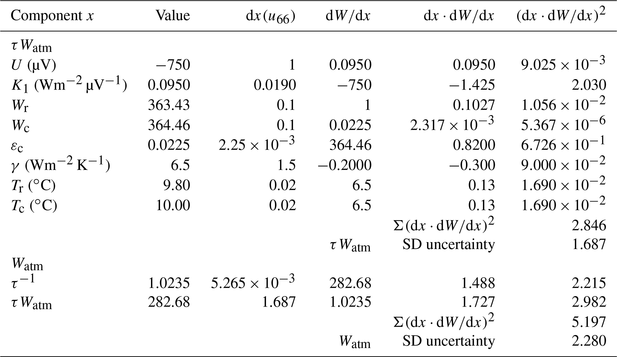
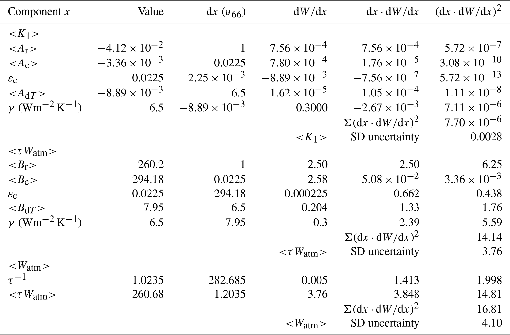
Based on the above assumptions, the components of uncertainty of a single measurement of W_atm using Eq. (18) are provided in Table 1. The dominant uncertainty components are K₁ and ε_c for the calculation of τW_atm, and the standard uncertainties for both τW_atm and τ make similar contributions to the uncertainty of W_atm.

Table 1 The standard uncertainty calculation for W_atm=289.33 Wm⁻² by calculation by Eq. (18). The first 11 component rows provide the calculation of the standard uncertainty for τW_atm, while the remaining rows provide the calculation of the standard uncertainty for W_atm. Apart from irradiance components (W_x) and dimensionless quantities ε_c and τ, the units of the components are provided in the first column.

8 New calibration methods

Four calibration methods will be examined below for ACP96 based at PMOD/WRC in Davos, Switzerland, using either characterisation data or comparison measurements with other reference IRIS pyrgeometers and implementing two versions of linear LSQ.

Based on the likely magnitudes of the uncertainties, assumed values for some parameters are used in all the calibration methods investigated below. The value of the cavity emissivity is fixed at 0.0225 using the NIST-derived value in Reda et al. (2012) for ACP95. The value for the backscatter from the concentrator β will be assumed to be 0.

Using blackbody investigations, two values of the convection coefficient have been estimated, 8.4 and 6.5. The latter value, 6.5, derived from early blackbody investigations and field measurements, produces convection-based irradiances closer to the equivalent “air cavity” irradiance values used by Reda et al. (2012). The logic behind this adjustment is not solely due to the convection coefficient being different, but rather the approximation T_c∼T_air.

This leaves the sensitivity of the thermopile K₁ and the concentrator transmission τ to be either assumed or provided by a characterisation methodology.

For the work reported below, the transmission of the concentrator τ is assumed to be only due to the construction of the concentrator and is independent of K₁. The values of τ for ACP95 derived by the reanalysis of the Zeng et al. (2010) data set but using Eq. (20) will be used when not derived as part of a calibration process.

The fraction of incoming terrestrial irradiance absorbed by the concentrator α_c is not independent of the concentrator ε_c. Concentrator transmission is a function of the cosine response of the concentrator, and ray tracing suggests that for most sky zenith angles there will be multiple reflections on its surface, and then α_c>ε_c. For ε_c=0.0225 derived by NIST as reported by Reda et al. (2012), the implication is that τ<0.9775.

For the results below when the method requires a fixed value of concentrator transmission, τ is set to 0.977 and a fixed estimate of ε_c=0.0225 and two values of the convection coefficient γ (8.4 and 6.5).

8.1 Data sets

During 2020 there were 242 d of ACP96 data collected at PMOD/WRC, and sometimes coincidentally with days, IRIS4 and or IRIS2 data were collected. Night-time data were available from ACP96 and IRIS2 between 7 January 2020 and 10 December 2020 and between 15 March and 10 December for IRIS4. The data consisted of an average value every 60 s for any IRIS irradiance and a 1 s measurement sequence every 10 s for ACP96. Simultaneous measurements were available in 2020, with 41 d of IRIS2 data and 36 d of IRIS4 that could be compared to ACP96.

Figure 1 shows a box–whisker representation of the differences between the simultaneous measurements of atmospheric terrestrial irradiances W_IRIS2 and W_IRIS4. The typical daily range in differences is 1.5 Wm⁻², which is within the individual instrument expanded uncertainty (k=2) of 2 Wm⁻² (Gröbner, 2021). Slightly larger differences, with IRIS2 lower than IRIS4, are observed on two days in August (days of the year 233 and 234), which are still within the combined uncertainties of the two radiometers. There appears to be a trend in the daily mean differences until day 260 and then a restoration of the early 2020 mean daily differences after day 300.

While there appears to be a drift between the two data sets, it was decided to use both data sets as a reference or comparison data set. These IRIS data tested the impact of using different reference irradiances and were used to corroborate the results of the methods described below.

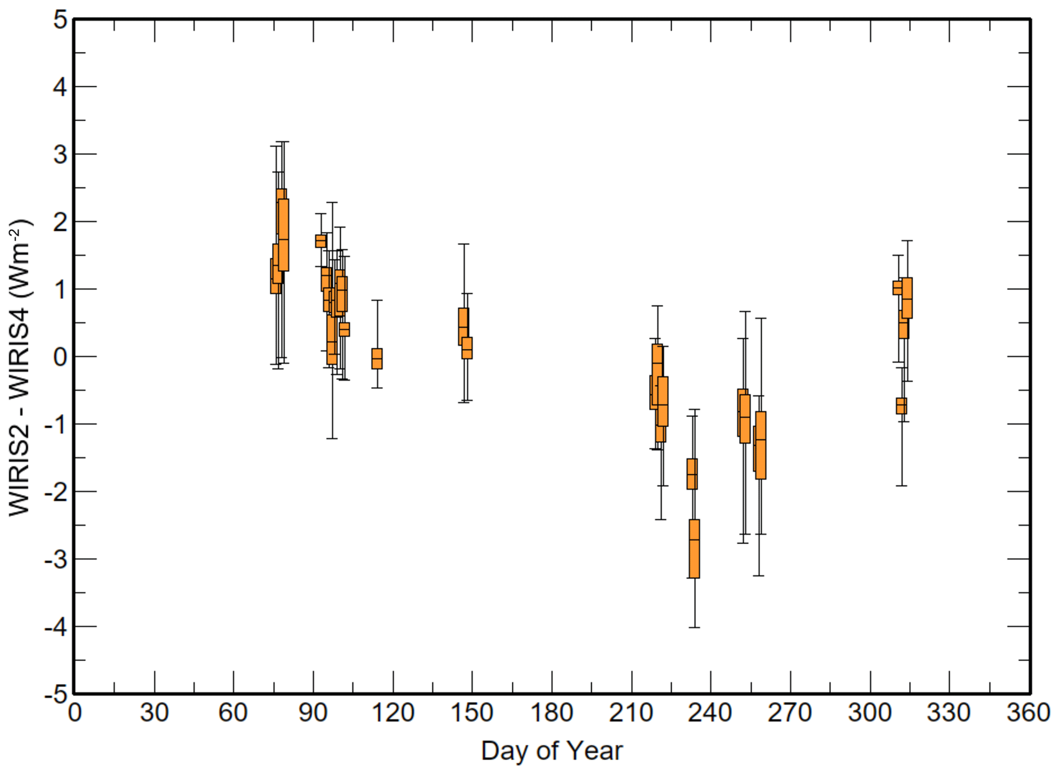
Figure 1 Statistics for the difference between W_IRIS2 and W_IRIS4 for every simultaneous irradiance in 2020 in box–whisker plots.

8.2 Deriving K₁ or C from an estimated solar calibration of the thermopile

For this method, either prior to an ACP being assembled or by removing the ACP's concentrator, the concentrator would be replaced with a pyrheliometer aperture system that conforms to pyrheliometer requirements, with the closest aperture to the receiver surface being identical to the aperture of the concentrator. The ACP would be pointed at the Sun and compared to a well-calibrated WRR (or SI) pyrheliometer to produce an estimate of the thermopile responsivity to solar irradiance. That estimate would then be converted to the infrared responsivity by assuming the emissivity of the receiver surface for both solar (ε_rsolar) and infrared emission (ε_r).

Unfortunately, no solar calibration exists for the thermopile of ACP96, so an estimate had to be made, and we will assume that the ACP thermopile responsivity for solar irradiance, C_solar, would likely be that of a new F3 thermopile and use the calibrations of new PSP pyranometers that were used to estimate a likely solar calibration for an F3 using an ACP. The data from over 82 individual PSP calibrations sourced from Eppley Laboratory and multiple national calibration centres in the USA, Canada and Australia indicated that the mode and mean solar sensitivities of new PSPs manufactured after 2000 were ∼9.3 µV (W⁻¹ m²).

An estimate for C is the effective responsivity of the thermopile receiver – µV (W⁻¹ m²):

$$\begin{array}{}\text{(24)}& C={\displaystyle \frac{{\mathit{\epsilon }}_{\mathrm{r}}{C}_{\mathrm{solar}}}{{\mathit{\tau }}_{\mathrm{dome}}^{\mathrm{2}}{\mathit{\epsilon }}_{\mathrm{rsolar}}}}.\end{array}$$

As Parsons Black is used to coat the receiver surface, with a typical receiver solar emissivity ε_rsolar∼0.98 and for infrared ε_r∼0.92, and a PSP has a double dome with both domes having a nominal transmission at solar wavelengths of τ_dome∼0.91, this then gives an estimate of C∼10.5 µV (W⁻¹ m²).

Using Eq. (18), the atmospheric irradiance W_APC96 was calculated when both IRIS4 and IRIS2 were operating and ACP96 was monitoring in steady-state night-time conditions. This resulted in comparisons over 41 nights (18 802 measurements) with IRIS2 and 33 nights (14 085 measurements) with IRIS4. The results are presented in Table 2 using C=10.5, γ=8.4, τ=0.977 and ε_s=0.0225; the daily mean differences (W_IRIS2−W_ACP96) and (W_IRIS2−W_ACP96) for each of the days are shown in Fig. 2. Similar statistics are presented in Table 2 and Fig. 3 using γ=6.5.

Table 2 The mean differences and the statistics of (W_IRIS2−W_ACP96) and (W_IRIS4−W_ACP96) (Wm⁻²) for data from January to November 2020, using C=10.5, γ=8.4, τ=0.977 and ε_s=0.0225.

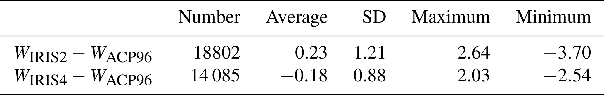
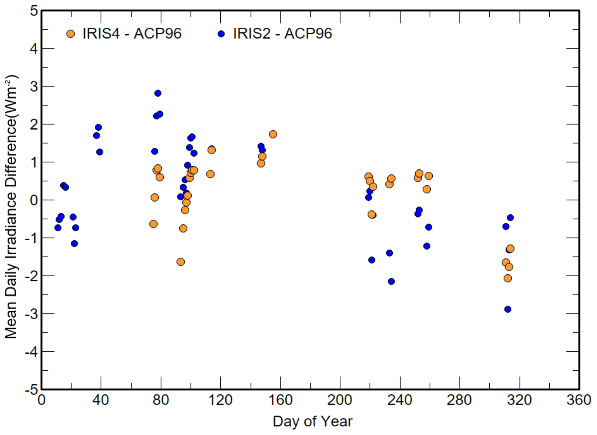
Figure 2 The daily mean differences and the statistics of (W_IRIS2−W_ACP96) and (W_IRIS4−W_ACP96) (Wm⁻²) from January to November 2020, using C=10.5, γ=8.4, τ=0.977 and ε_c=0.0225.

Table 3 The mean differences and the statistics of (W_IRIS2−W_ACP96) and (W_IRIS4−W_ACP96) (Wm⁻²) for data from January to November 2020, using C=10.5, γ=6.5, τ=0.977 and ε_c=0.0225.

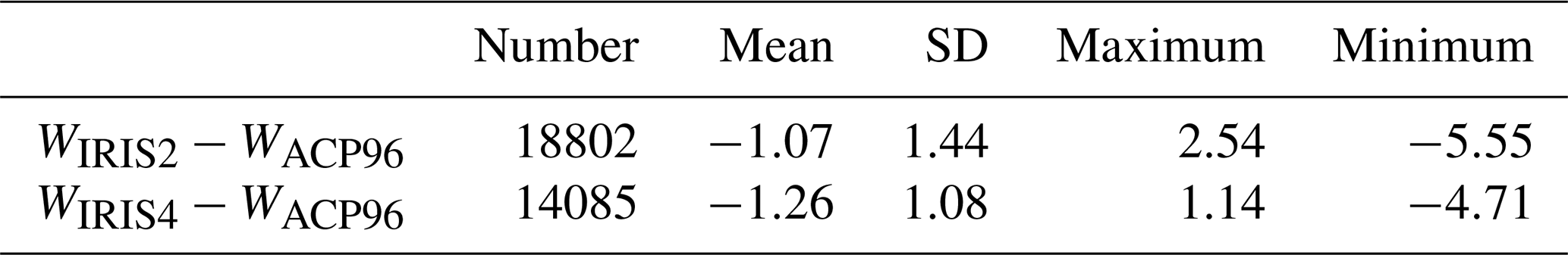
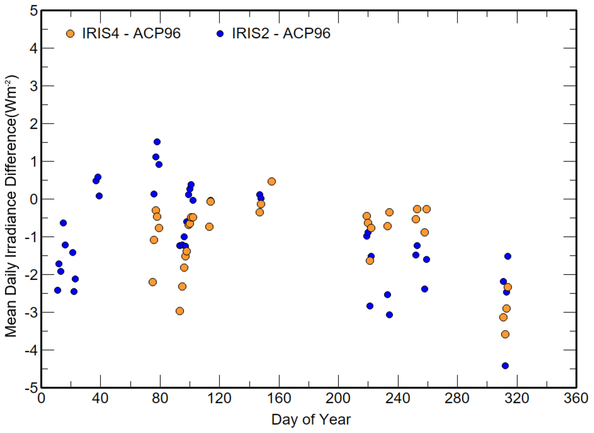
Figure 3 The daily mean differences and the statistics of (W_IRIS2−W_ACP96) and (W_IRIS4−W_ACP96) (Wm⁻²) from January to November 2020, using C=10.5, γ=6.5, τ=0.977 and ε_c=0.0225.

The differences to W_IRIS2 were larger than for W_IRIS4, and there appears to be a similar trend in the relationship between IRIS2 and ACP96, as seen in the comparison between W_IRIS2 and W_IRIS4. The differences between Table 2 and Table 3 show that the impact of a 22 % change in γ for steady-state conditions is a 0.6 Wm⁻² APC96 irradiance difference for Δγ=1. Decreasing γ by −1.9 shifted all the mean values down by ∼1.2 Wm⁻² but increased the range of the W_IRIS2−W_ACP96, while the W_IRIS4−W_ACP96 showed little change.

8.3 Outdoor calibration using a reference irradiance

This method also assumes fixed values for the concentrator emissivity ε_c and convection coefficient γ and finds the minimum difference between the reference irradiance W_IRIS2 or W_IRIS4 and W_ACP96 using paired values of K₁ and concentrator transmission τ. That is, for a set of n observations made up of m nights, ideally with ranges in W_IRIS and W_ACP96, the pair [C, τ] is found that provides a mean difference of (W_IRIS−W_ACP96) of less than 0.1 Wm⁻². Given the low irradiance impact of concentrator emissivity and the convection coefficient in steady-state conditions, the convergence to a solution is straightforward.

In the γ=8.4 set, the (W_IRIS−W_ACP96) statistics for simultaneous measurements with IRIS2 and IRIS4 observations are presented in Table 4. There are differences of 0.4 (or ∼4 %) between the C values and 0.011 (∼1.2 %) between the resultant concentrator transmission values. The table also presents the results of using the average of the two C and transmission values derived from IRIS2 and IRIS4, giving C=10.5 and τ=0.9764 and deriving the difference statistics to both IRIS2 and IRIS4.

Table 4 The statistics of (W_IRIS−W_ACP96) using ε_c=0.0225 and γ=8.4 from March to November 2020, for the pairs of C and τ that minimised the mean difference of W_IRIS−W_ACP96. The difference statistics using the average C and τ of the IRIS2 and IRIS4 results are also given in the last two rows of the table.

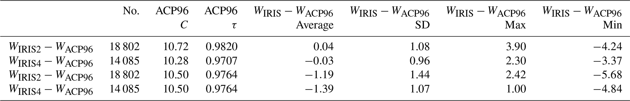
If the three C values in Table 4 are converted to equivalent PSP F3 thermopile solar C_solar values, this results in values centred on 9.35±0.3.

The process was repeated but using a convection coefficient γ of 6.5, with the results presented in Table 5. The standard deviations and range of differences increase slightly when compared to the values derived using 8.4 for the convection coefficient. The resultant C values were reduced by 0.2, while the transmission values are reduced by ∼0.0013.

Table 5 The statistics of (W_IRIS−W_ACP96) using ε_c=0.0225 and γ=6.5 from March to November 2020, for pairs of C and τ that minimised the standard deviation of (W_IRIS−W_ACP96). The difference statistics using the average C and τ of the IRIS2 and IRIS4 results are also given in the last two rows of the table.

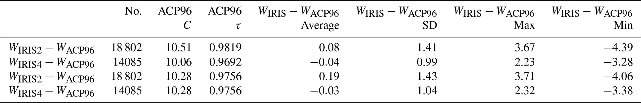
The results in Tables 4 and 5 indicate that a negative 22 % change in the convection coefficient reduces C by 2 % and increases the transmission by 0.1 % to achieve mean irradiance differences of less than 0.1 Wm⁻². These changes are self-consistent given the high correlation between the components of the ACP equations, either of Reda et al. (2012) or the new equation, and show a 2 Wm⁻² impact with a change in the convection component of 1.9. However, for the averaged values of C and transmission, the lower convection coefficient provided the averages closest to 0 for both reference irradiances. The transmissions in Tables 4 and 5 from using the mean of the IRIS2 and IRIS4 results are within 0.002 of the 0.977 value derived for ACP95 using the new equation and NIST laboratory measurements (Zeng et al., 2010).

The small differences (W_IRIS2−W_IRIS4) for 2 d in August and the high correlation between components in the new equation demonstrate that uncertainty in the reference irradiance impacts the minimisation method and shows the benefit of having multiple reference irradiances to assess confidence intervals.

The increase in C with an increase in transmission and the magnitude of these changes is a consequence of the difference in the measured W_IRIS2 and W_IRIS4. The two dominant components of W_atm using the new equation are the thermopile voltage and the thermopile blackbody irradiance W_r; the contributions from W_c and (T_r−T_c) are less than 4 %. The magnitude of the irradiance derived from the thermopile signal is of the order of −80 Wm⁻², while W_r is typically between 300 and 500 Wm⁻². Hence, if the minimisation method is to achieve a balance between K₁ and transmission, for a 1 Wm⁻² change in reference irradiance, then K₁ changes by the higher percentage as the W_r is unchanged. If only K₁ was minimised instead of a (K₁, τ) pair, then a Δ Wm⁻² difference in W_atm would result in K₁ changing by $\mathrm{\Delta }/W_{\mathrm{r}}$. Further complications arise if the relationship between the true W_atm and W_ref changes.

8.4 Adaption of the Reda et al. (2012) linear LSQ calibration method to the new equation

From Eq. (18), and assuming that the fraction of backscatter of incoming irradiance β is 0, we can define the predictand for the linear LSQ analysis as

$$\begin{array}{}\text{(25)}& \begin{array}{rl}& y\left(W_{\mathrm{r}},W_{\mathrm{c}},T_{\mathrm{r}},T_{\mathrm{c}},t\right)=W_{\mathrm{net}}\left(t\right)=W_{\mathrm{r}}\left(t\right)-{\mathit{\epsilon }}_{\mathrm{c}}{W}_{\mathrm{c}}\left(t\right)\\ & +\mathit{\gamma }(T_{\mathrm{r}}\left(t\right)-T_{\mathrm{c}}\left(t\right)),\end{array}\end{array}$$

with the thermopile voltage V the predictor for the linear LSQ analysis, and hence the equation to solve by linear LSQ is

$$\begin{array}{}\text{(26)}& \begin{array}{rl}& y\left(W_{\mathrm{r}},W_{\mathrm{c}},T_{\mathrm{r}},T_{\mathrm{c}},t\right)=W_{\mathrm{net}}\left(t\right)=<\mathit{\tau }{W}_{\mathrm{atm}}>\\ & -<K_{\mathrm{1}}>\mathrm{V}\left(t\right),\end{array}\end{array}$$

which results in $\mathit{<}C\mathit{>}=\mathrm{1}/\mathit{<}{K}_{\mathrm{1}}$ and is independent of concentrator transmission. From <τW_atm>, assuming a value for the concentrator transmission results in values for <W_atm> which could be compared to a reference irradiance. The inverse would be to prescribe a reference irradiance and derive a concentrator transmission.

For the linear LSQ process to be successful, W_atm and γ must be constant during the data collection process and the ACP equation must be valid. In stable W_atm conditions, the process for collecting the required rapid cooling periods results in only small changes in T_c and W_c. As a result, the changes in the concentrator irradiance component ε_cW_c are less than 0.1 Wm⁻² over the entire rapid cooling process and hence have a minimal impact on <K₁>.

Given the properties of linear LSQ, using a single predictor, V(t), if the predictand is made up of multiple linear components, one can solve for each component of the predictands independently. The three predictand components from Eq. (18) are

$$\begin{array}{}\text{(27)}& W_{\mathrm{r}}\left(t\right)=y_{\mathrm{r}}\left(t\right)=<A_{\mathrm{r}}>\mathrm{V}\left(t\right)+<B_{\mathrm{r}}>.\end{array}$$

Similarly,

$$\begin{array}{}\text{(28)}& W_{\mathrm{c}}\left(t\right)=y_{\mathrm{c}}\left(t\right)=<A_{\mathrm{c}}>\mathrm{V}\left(t\right)+<B_{\mathrm{c}}>,\end{array}$$

and lastly,

$$\begin{array}{}\text{(29)}& \begin{array}{rl}\mathrm{d}T\left(t\right)& =\left(T_{\mathrm{r}}\left(t\right)-T_{\mathrm{c}}\left(t\right)\right)=y_{\mathrm{d}T}\left(t\right)=<A_{\mathrm{d}T}>\mathrm{V}\left(t\right)\\ & +<B_{\mathrm{d}T}>.\end{array}\end{array}$$

dT(t) can also be split into three separate components, but that will be left to the discussion section of this paper on the impact of incorrect estimates of the Seebeck coefficient and assuming T_c(t) is equivalent to T_air(t).

Derived <K₁> and <τW_atm> using the new equation are given by

$$\begin{array}{}\text{(30)}& <K_{\mathrm{1}}\mathit{>=}<{\displaystyle \frac{\mathrm{1}}{C}}\mathit{>=}{\mathit{\epsilon }}_{\mathrm{c}}<A_{\mathrm{c}}>-<A_{\mathrm{r}}>-\mathit{\gamma }<A_{\mathrm{d}T}>\end{array}$$

and

$$\begin{array}{}\text{(31)}& \mathit{\tau }<W_{\mathrm{atm}}\mathit{>=}<B_{\mathrm{r}}>-{\mathit{\epsilon }}_{\mathrm{c}}<B_{\mathrm{c}}>+\mathit{\gamma }<B_{\mathrm{d}T}>.\end{array}$$

Given that W_c is almost constant through the ∼7 min cooling of the thermopile and $\left|\mathit{<}{A}_{\mathrm{c}}\mathit{>}\right|\mathit{<}\mathrm{0.005}$, then $\left|{\mathit{\epsilon }}_{\mathrm{c}}\mathit{<}{A}_{\mathrm{c}}\mathit{>}\right|\mathit{<}\mathrm{0.00015}$ and contributes less than 0.1 % to <K₁>, and hence the concentrator emissivity has minimal impact on deriving <K₁> using the new equation. For the intercept terms, ε_c<B_c> typically makes a small negative contribution to <τW_atm> of the order of 2.5 %. W_r and (T_r−T_c) dominate contributions to both <K₁> and <τW_atm>.

The concentrator transmission is irrelevant to deriving <τW_atm> or <K₁> but is essential for estimating <W_atm> from <τW_atm>. If W_atm is known through a reference radiometer (W_ref), then the concentrator transmission can be estimated by

$$\begin{array}{}\text{(32)}& \mathit{\tau }={\displaystyle \frac{<\mathit{\tau }{W}_{\mathrm{atm}}>}{W_{\mathrm{ref}}}}.\end{array}$$

For any linear LSQ process there is a key requirement that the process is linear, and for Eq. (18), τW_atm must be constant. As a result, initial criteria for acceptable conditions were established for a valid linear LSQ analysis period.

When the base of the ACP is cooled rapidly, the thermopile signal must continuously become less negative. As the thermopile voltage was measured every 10 s, a valid time was defined when the following criteria were met. (a) The difference in consecutive thermopile voltages was more than +3.5 µV. (b) The difference in consecutive (T_r(t)−T_c(t)) was less than −0.04 K. (c) The total range of the voltage was greater than 200 µV. (d) ($T_{\mathrm{r}}-T_{\mathrm{c}}\left)\right(t_i)-(T_{\mathrm{r}}-T_{\mathrm{c}}\left)\right(t_{i-\mathrm{1}})\mathit{<}\mathrm{0.02}$. These ensured that the cooling was not nearing the new base temperature or that cooling had stopped.

Out of 266 possible periods during 2020 for ACP96, 244 linear LSQ calibration periods satisfied the criteria. Figures 4 to 5 show the time series of the individual slopes <A_c>, <A_r> and <A_dT> and intercepts (<B_r>, <B_c> and <B_dT>) derived from the valid linear LSQ analyses. <A_c> and <A_r> are stable about a mean value but not the slopes for (T_r−T_c) and <A_dT>; meteorological data for these periods indicate that the dew point temperature was less than 4 K below the ambient temperature and that thermopile surface temperatures during cooling were close to or less than the dew point. While <B_dT> is relatively constant over the year, as expected, <B_r> and <B_c> follow the irradiance of the ambient temperature peaking in summer periods.

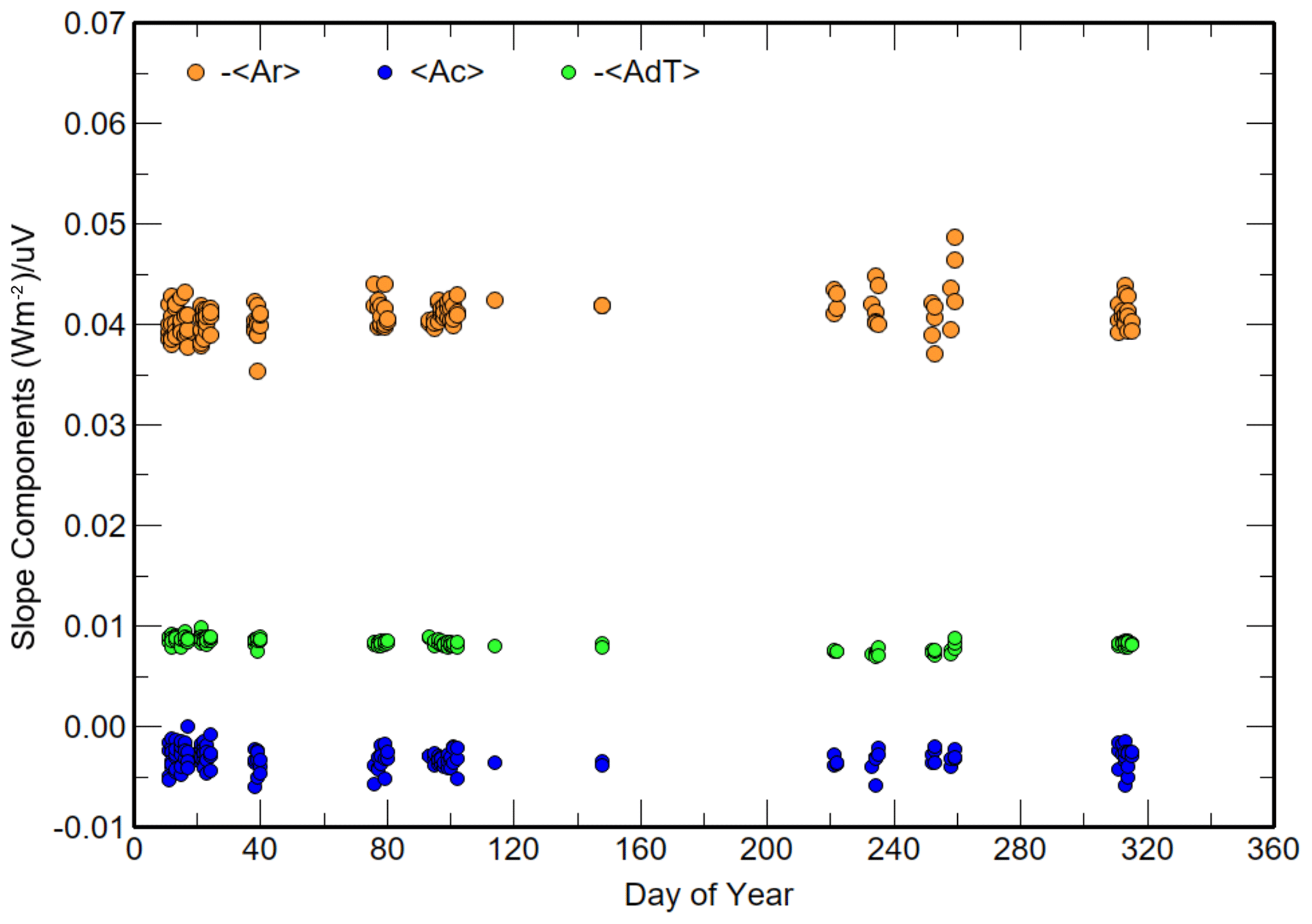
Figure 4 The linear LSQ slope <A_r>, <A_c> and <A_dT> components that generate <K₁> for 244 calibrations in 2020.

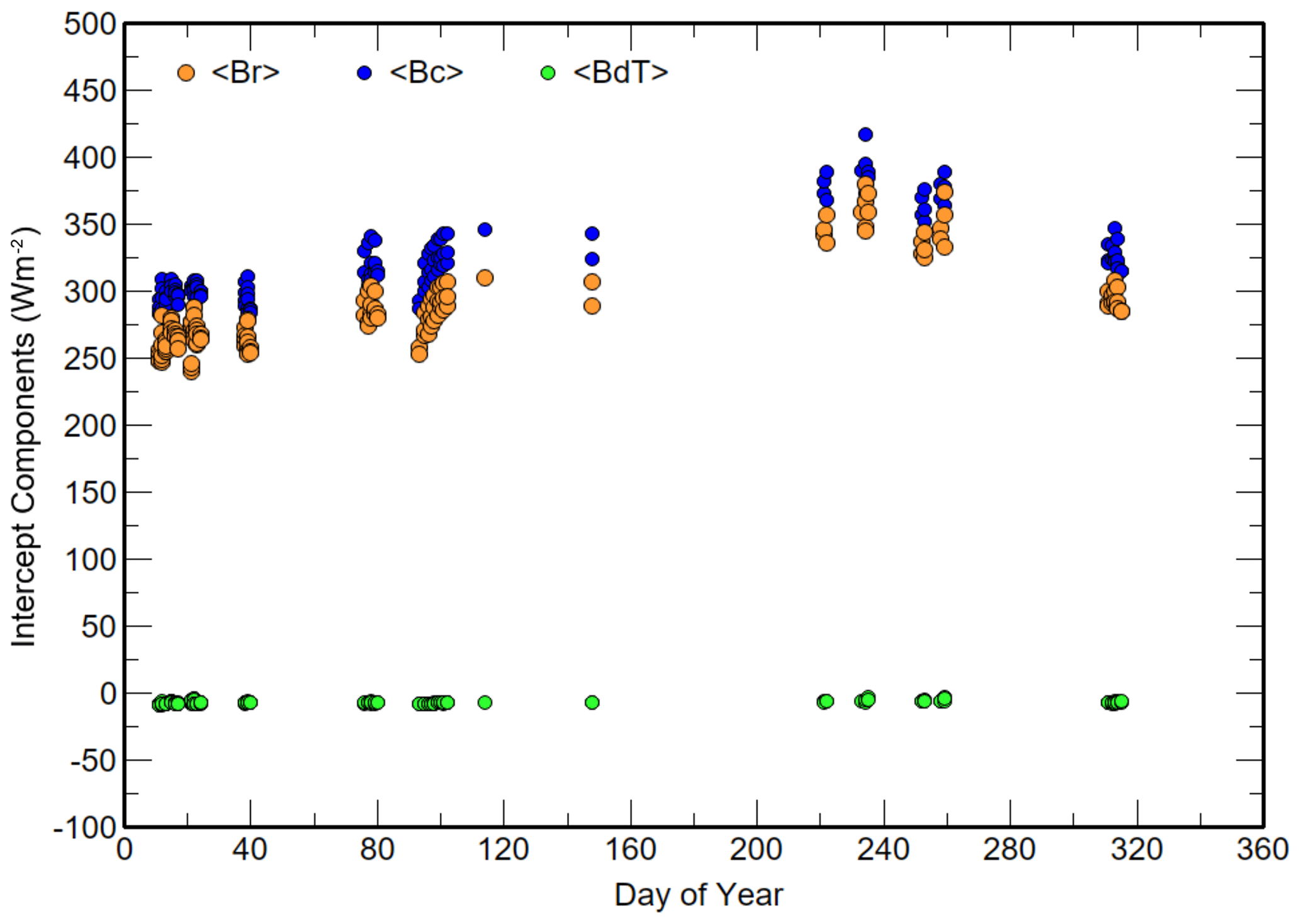
Figure 5 The linear LSQ slope <B_r>, <B_c> and <B_dT> components that generate <τW_atm> for 244 calibrations in 2020.

The thermopile responsivities <C> found for 244 linear LSQ calibration periods are shown in Fig. 6. Between days 210 and 260 there is a significant increase in the range of <C> compared to the rest of the year.

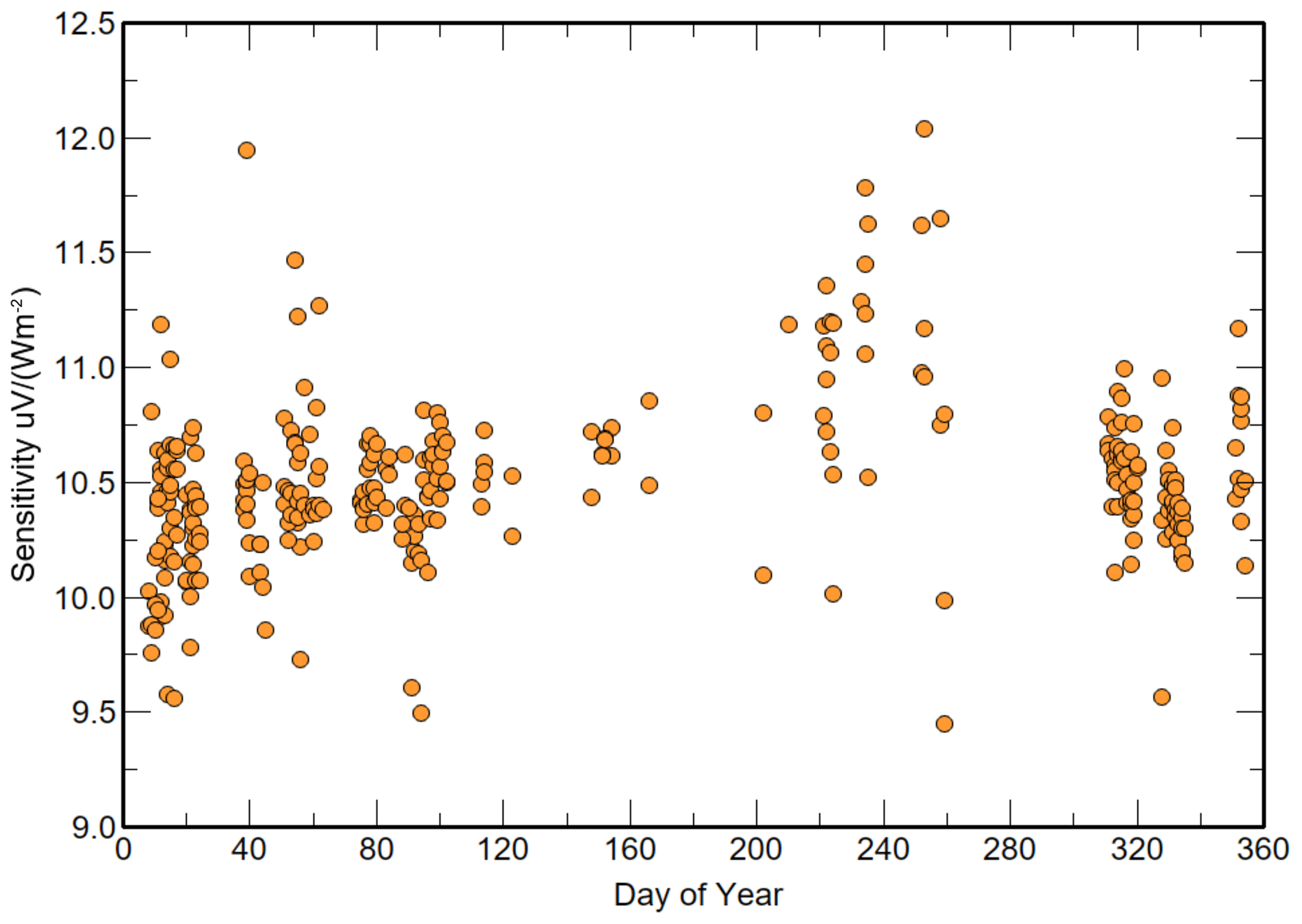
Figure 6 ACP96 < C> values derived using the new equation using the linear LSQ method with ε_c=0.0225 and γ=6.5 for 244 calibration periods in 2020.

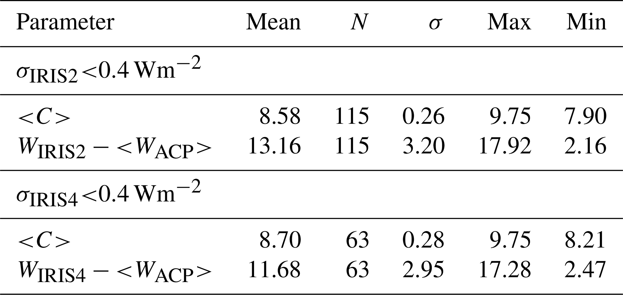
There were 115 periods that were coincident with IRIS2 measurements when the standard deviation of W_IRIS2 in a cooling sequence was less than 0.4 Wm⁻², and 63 were coincident with IRIS4, also with a standard deviation of less than 0.4 Wm⁻². <C> statistics for the 244 linear calibration periods and irradiance differences for the coincident periods with W_IRIS2 or W_IRIS4 are presented in Tables 6 and 7 for γ=6.5 and γ=8.4 respectively.

Table 6 Linear LSQ method results for ACP96 < C> using ε_c=0.0225, γ=6.5 and τ=0.977 and the difference between ACP96 and IRIS irradiances when coincident data were available (W_IRIS−<W_atm>). <C> statistics for all 244 linear LSQ calibrations are presented in the first data row. The second and third data rows concern periods when ACP96 and IRIS2 data were available; the fourth and fifth data rows concern periods when ACP96 and IRIS4 were available. The last data row gives the statistics of the irradiance differences between the two IRIS radiometers for 63 d of coincident data.

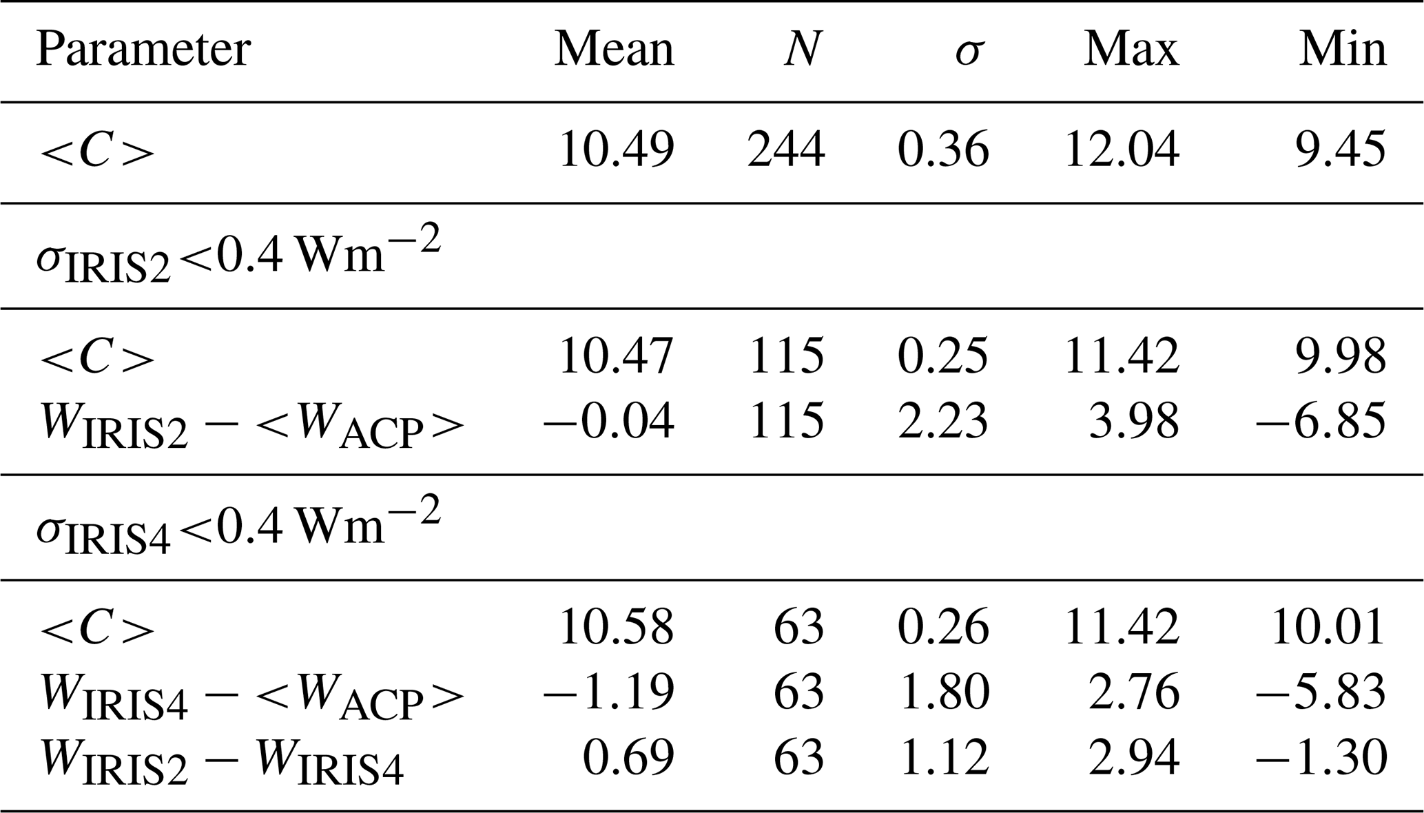
Table 7 Linear LSQ method results for ACP96 < C> using ε_c=0.0225, γ=8.4 and τ=0.977 and the difference between ACP96 and IRIS irradiances when coincident data were available (W_IRIS−<W_atm>). The first and second data rows concern periods when ACP96 and IRIS2 data were available; the third and fourth data rows concern periods when ACP96 and IRIS4 were available.

The differences (W_IRIS2−<W_atm>) and (W_IRIS4−<W_atm>) for coincident measurements using a convection coefficient of 6.5 are shown in Fig. 7. The results between days 200 and 254 for both <C> and <W_atm> appear to be anomalous, with significantly higher values of <C> and underestimates of the irradiance differences; these are during periods when the steady-state base temperature is typically high for the year and within 4 K of the dew point temperature and high relative humidity of 80 %. The means of pre day 200 and post day 300 are separated by about 2.2 Wm⁻². Given that <C> is likely constant over the two periods, possible reasons for the 2.2 Wm⁻² irradiances are that (i) both reference IRIS irradiances' calibrations may have changed by the same amount, (ii) the transmission of the concentrator may have decreased and (iii) the use of a constant convection coefficient over the entire year is inappropriate.

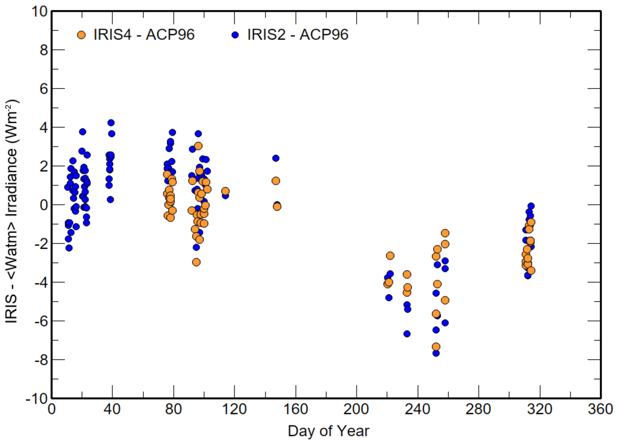
Figure 7 Daily mean irradiance differences (W_IRIS−<W_atm>) between the mean IRIS (W_IRIS) and linear LSQ-interpolated ACP96 (<W_atm>), using the new equation with ε_c=0.0225, γ=6.5 and τ=0.977.

The mean derived <C> value in Table 5 using 6.5 as the convection coefficient is 10.49 µV (W⁻¹ m²), which is within 0.3 µV (W⁻¹ m²) of the solar and minimisation methods. Table 7 using the higher convection coefficient of 8.4 shows a mean C about 18 % lower and irradiance differences greater than 11 Wm⁻² between the ACP96 and IRIS2 and IRIS4.

No attempt was made to adjust the concentrator transmission τ based on the derived <C> (or K₁), as it is a property of the concentrator, not the thermopile. However, it was possible to estimate τ using the derived <τW_atm> from the linear LSQ intercept, which is independent of any assumed value of τ by dividing <τW_atm> by W_IRIS4. Similarly, the derived <τW_atm> from the Reda et al. (2012) equation could also produce an estimate of the concentrator transmission τ. Figure 8 shows the results of dividing the <τW_atm> derived from both LSQ equations by IRIS4 data. Similar results were obtained using W_IRIS2. The results using the new equation suggest a concentrator transmission τ∼0.98, while for the Reda et al. (2012) equation a significant majority of periods gave unphysical values of τ greater than 1.

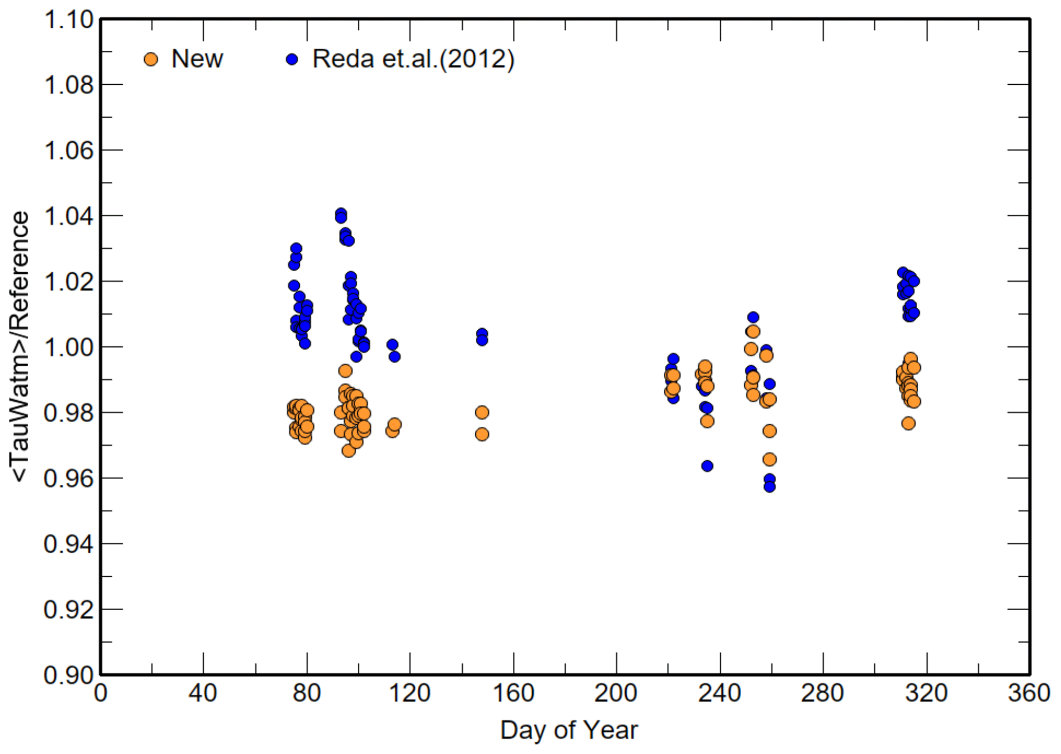
Figure 8 Concentrator transmission estimates derived from dividing the linear LSQ-obtained <τW_atm> by W_IRIS4 for 63 estimates using the new Eq. (18) and the Reda et al. (2012) Eq. (22) estimate of <τW_atm>.

8.5 Ensuring the representativeness of τW_atm during a linear LSQ calibration period

The thermopile voltage measurement is a consequence of net irradiance based on the temperature difference between the base of the thermopile and the top of the thermopile. The blackbody equivalent irradiance of the thermopile receiver is calculated by assuming that the Seebeck coefficient is valid and that the body temperature represents the temperature at the base of the thermopile. Provided the time constants of the thermopile and thermistors are similar and the heating and cooling of the body are not too rapid, C and the convection coefficient should provide τW_atm for all measurements (or K₁ in Eq. 22) and ideally produce a near-constant value during both cooling and heating.

Using the data for ACP96 in 2020 and the calculated mean values of C given in Table 6, τW(t) was generated for each cooling and heating period. τW_atm(t) was found to maintain some repeatable oscillations that could not be minimised by changing either the convection coefficient or C for the new equation. For the Reda et al. (2012) equation, only K₁ could be varied and resulted in decreases in calculated irradiances over the cooling and heating period regardless of the K₁ used, with little if any impact on deviations from a presumably constant τW_atm.

The sinusoid shape of the oscillation in the derived τW_atm using Eq. (18) gave higher values during cooling and lower values during heating, suggesting that there was a phase difference between the thermopile voltage and the body temperature or that some processes were unaccounted for using the new equation. If a phase issue, the thermopile voltage at measurement period p was lagging the changing body temperature, and hence the temperature of the body at time t was not representing the temperature of the thermopile base at t. Such differences would be tiny in steady-state conditions given the slow rate of change in T_b.

Linear interpolation in time was used to find a more representative thermopile voltage that reduced the sinusoidal oscillation in the derived τW_atm and found that for ACP96 a lag time of about 9 s ± 2 s was required to reduce the magnitudes of oscillations about the mean when using the new equation's τW_atm. It also reduced the magnitude of the difference from the constant τW_atm using the Reda et al. (2012) equation, but a distinct sinusoid always remained with peak deviations of 2 Wm⁻² or more but 180^∘ out of phase with the new equation values.

Given that measurements for all quantities were repeated every 10 s, the most representative thermopile voltage for measurement p every 10 s, ${\mathrm{V}}_{p^{\prime }}$, was

$$\begin{array}{}\text{(33)}& {\mathrm{V}}_{p{}^{\prime }}={\mathrm{V}}_p+\mathrm{0.9}({\mathrm{V}}_{p+\mathrm{1}}-{\mathrm{V}}_p).\end{array}$$

Using this interpolated voltage ${\mathrm{V}}_{p^{\prime }}$ to represent the thermopile voltage at p resulted in significantly improved standard errors and confidence intervals for each of the linear LSQ-derived components of <K₁> and <C> by factors of 3 to 10 depending on the linear LSQ component and provided statistics for the variation of τW_atm throughout each cooling and heating period. The improved linear LSQ fits did not impact significantly the derived <K₁> or <C>, only raising <C> by less than 0.02, with no significant difference to the results presented in Sect. 8.4.

Using Eq. (33) to represent the thermopile signal for measurement p and setting a maximum standard deviation limit of τW_atm over the cooling and heating period of 0.6 Wm⁻² as acceptable when using the new equation, the results for <C> derived by linear LSQ in Sect. 8.4 were re-examined. Figure 10 shows the same <C> values as in Fig. 7 and those that satisfy the standard deviation of the τW_atm criterion. Of the 244 original values, only 51 had a larger standard deviation in τW_atm over the cooling period. The main impact of this limit was removal of outliers. It had little impact on the divergence of results between days 200 and 260 in 2020.

The phase shift showed that both the new and Reda et al. (2012) equations could represent τW_atm through the cooling and heating with varying degrees of success. A cumbersome visual method showed that varying the convection coefficient constant for each cooling and heating cycle further reduces the sizes of the deviations from τW_atm and was not independent of the estimate for C, but this is not the subject of the current paper. Most importantly, automation of the visual method may provide a method of judging whether τW_atm was nominally constant during a linear LSQ calibration period and thus remove the requirement of a reference radiometer for that purpose.

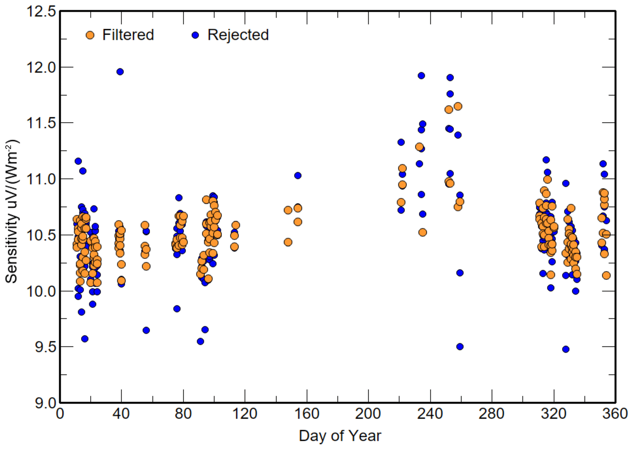
Figure 9 Responsivity <C> values presented in Fig. 6 but filtered for standard deviations of ACP96 τW_atm during the cooling and heating period that are less than 0.6 Wm⁻² are in gold, and those with higher standard deviations are in blue.

9 Discussion

The four different methods using the new ACP irradiance equation to calibrate the ACP96 provided irradiances that compared well with the irradiances from IRIS2 and IRIS4 during 2020. One based on laboratory or blackbody estimates for concentrator emissivity, transmission and the convection coefficient provided an estimate of C based on the modal value of 80 new F3 thermopile solar calibrations. Another used minimisation of the differences between the ACP and IRIS radiometers for pairs of C and concentrator transmission. The third used the new equation with the linear LSQ of Reda et al. (2012) but treated every contributor separately. The fourth used the derived calibrations in the third method to estimate τW_atm from every measurement during a cooling and heating period and thereby filter the results for stable periods without the need for a separate pyrgeometer. All the methods produced mean differences from IRIS2 and IRIS4 of less than 1.2 Wm⁻² and typically ranges of ±3 Wm⁻² from the mean difference for IRIS4. The differences in irradiances between IRIS2 and ACP96 were not symmetric about the mean, suggesting an identical trend in the calibration of either both ACP96 and IRIS4 simultaneously or just IRIS2. As the year progressed, the daily mean differences between IRIS2 and ACP96 became increasingly negative until day 300, when irradiances recovered and equated to IRIS4 as during March and April 2020.

That the pseudo-solar calibration method produced a value very close to the other methods was fortuitous given that it was based on the modal value of initial PSP calibrations based on 82 instruments. The range of potential values matched the derived results and suggests that a solar calibration of the ACP F3 thermopile is both a useful first step in characterising an ACP thermopile as well as estimating the maximum potential ACP C calibration, and the method could be used periodically to check the stability of the thermopile. An extended solar calibration over ambient temperature ranges using the method of Pascoe and Forgan (1980) could also confirm the temperature compensation of the thermopile. However, given the decadal decrease in responsivity of the F3 thermopiles in PSP radiometers, exposure of an ACP thermopile to solar exposure should be kept to a minimum to reduce the impact of solarisation of the Parsons Black paint. Using the solar method as a primary calibration also negates the ACP as an absolute irradiance reference standard and is based on historical estimates of the emissivity of Parsons Black in both the IR and solar wavelengths. However, as most World Meteorological Organization regional instrument centres have ready access to well-maintained reference pyrheliometers but do not have laboratory facilities to characterise the concentrator, solar calibrations could be a useful verification and monitoring tool. At a minimum, the solar calibration will provide a lower limit for K₁ (and hence an upper limit for C). That the theoretical value derived from the nominal solar calibration from an ensemble of new PSP F3 thermopiles gave mean deviations of less than 1.5 Wm⁻² for over 14 000 measurements with a standard deviation of ∼1 Wm⁻² supports this recommendation.

The second method used an IR reference irradiance using IRIS pyrgeometers to solve for both C and concentrator transmission simultaneously. The reference pyrgeometers, both IRIS, are not influenced by calibration coefficients dependent on the spectral transmission and emission of the IR of the domes. However, it was clear from the 2020 comparison data that any reference radiometer must have an up-to-date calibration, with distinct steps and trends in the derived relationship between the ACP and IRIS radiometers in the comparison data. However, irradiance differences are all well within the current WMO traceability requirement for terrestrial irradiances of 5 Wm⁻².

The concentrator transmission derived for ACP95 using the data from Zeng et al. (2010) but the new equation and the NIST value of concentrator emissivity reported by Reda et al. (2012) were applied to ACP96 and produced good agreement with the IRIS2 and IRIS4 measurements regardless of the methods described above. This suggests that these parameters could be used as a first approximation for any ACP. If an ACP is to be used without reference to a black body or a reference radiometer, the concentrator emissivity should be obtained independently in the laboratory using the laboratory techniques reported by Reda et al. (2012), and the impact of a significant error in the emissivity for any irradiance calculation by the new equation would be small. However, as the difference between the true versus assumed concentrator transmissions will have a directly proportional effect on W_atm, an alternative method to obtain the concentrator emissivity would be to repeat the Zeng et al. (2010) methodology for each ACP using the new equation to generate a concentrator transmission and then assume the emissivity is (1−τ).

By deriving τW_atm from each measurement in a cooling and heating calibration period, the phase lag between the cooling of the base and the base of the thermopile became clear. The distance between where the base temperature is measured and the base of the thermopile is about 10 mm, and during the calibration periods the delay in the response of the thermopile base was found to be about ∼9 s for ACP96. Including that phase lag in the linear LSQ methods improved the confidence intervals for each linear LSQ analysis by factors of 3 to over 10 but had little impact on the derived gradients and intercepts. However, it did improve the measurement estimate of τW_atm from individual measurements and provided a method to estimate the variance of τW_atm during a calibration period without the need for a reference radiometer.

The comparisons between the IRIS and ACP irradiances in the results above suggest that the ACP thermopile was stable over the year and produced irradiance ratios to a reference within 2 % over 2020 and with a maximum difference of 5 Wm⁻². Reda et al. (2012) stated that the linear LSQ <K₁> value from a single linear LSQ calibration period be used as the valid sensitivity for the period between the end of the heating period that generated the linear LSQ value until the next LSQ calibration period, usually within 3 h. The results from Reda et al. (2012) and the results presented above for ACP96 suggest that during a single night of linear LSQ calibrations the derived <K₁> can vary by more than ±5 %, yet the typical F3 thermopile is found to be stable well within ±2 % over years for both solar and IR measurements. In other radiometric linear LSQ calibration methods, mean or mode statistics of several linear LSQ calibrations are used to reduce uncertainty in calibrations on the assumption that <C> is a constant. The results above support using a C that represents a mean or mode resulting from more than 20 calibration periods spread over several nights.

9.1 Uncertainty in the Seebeck coefficient using linear LSQ

The equation from Reda et al. (2012) and the new equation are dependent on the estimate of the Seebeck coefficient S in Eq. (7). A fixed value of $\mathrm{7.044}\times {\mathrm{10}}^{-\mathrm{4}}$ was used in the analysis above. In steady-state conditions when measuring the incoming irradiance, the impact of any offset from the true value is likely minor provided the other coefficients in the new equation have low uncertainties.

The Seebeck coefficient has a direct influence on both the W_r term and the (T_r−T_c) term of the new equation. For the (T_r−T_c) term, the impact is straightforward given Eq. (7) in that, if the error in the Seebeck coefficient is ΔS, then the contributory error is Δγ for <K₁> and <τW_atm>. The impact of any error in S is slightly more complicated for W_r, but the ACP96 2020 data suggest similar impacts. This is shown in Fig. 10 plotting the difference in <K₁> when ignoring S in the <A_r> term. The difference was calculated by subtracting the receiver slope assuming S=0, that is, base irradiance slope <A_b>, from the slope derived using S. The difference changes through the year inversely to the magnitude of the base temperature, but on average it is $\sim -\mathrm{0.0033}$ or about −4 % of <K₁>, which implies that a 25 % error in S has an impact of 1 % on <K₁>.

For the Reda et al. (2012) equation, the impact of the Seebeck coefficient is nearly doubled, as the scaling factor is (2−ε_c) instead of 1 for the new equation.

Figure 10 The difference in the receiver irradiance slope <A_r> and the slope by assuming the Seebeck coefficient is 0 <A_b> when deriving <K₁> from the linear LSQ slope.

9.2 Comparing <C> and <τW_atm> using the Reda et al. (2012) equation and the new equation

Isolating the coefficients that impact the derived <K₁> via linear LSQ also allows the calculation of the <K₁> value based on the Reda et al. (2012) equation. Figure 11 shows the two components in Eq. (22) after applying the scaling factors to generate <K₁>; in essence, W_r dominates the calculation, with a small negative contribution from W_c.

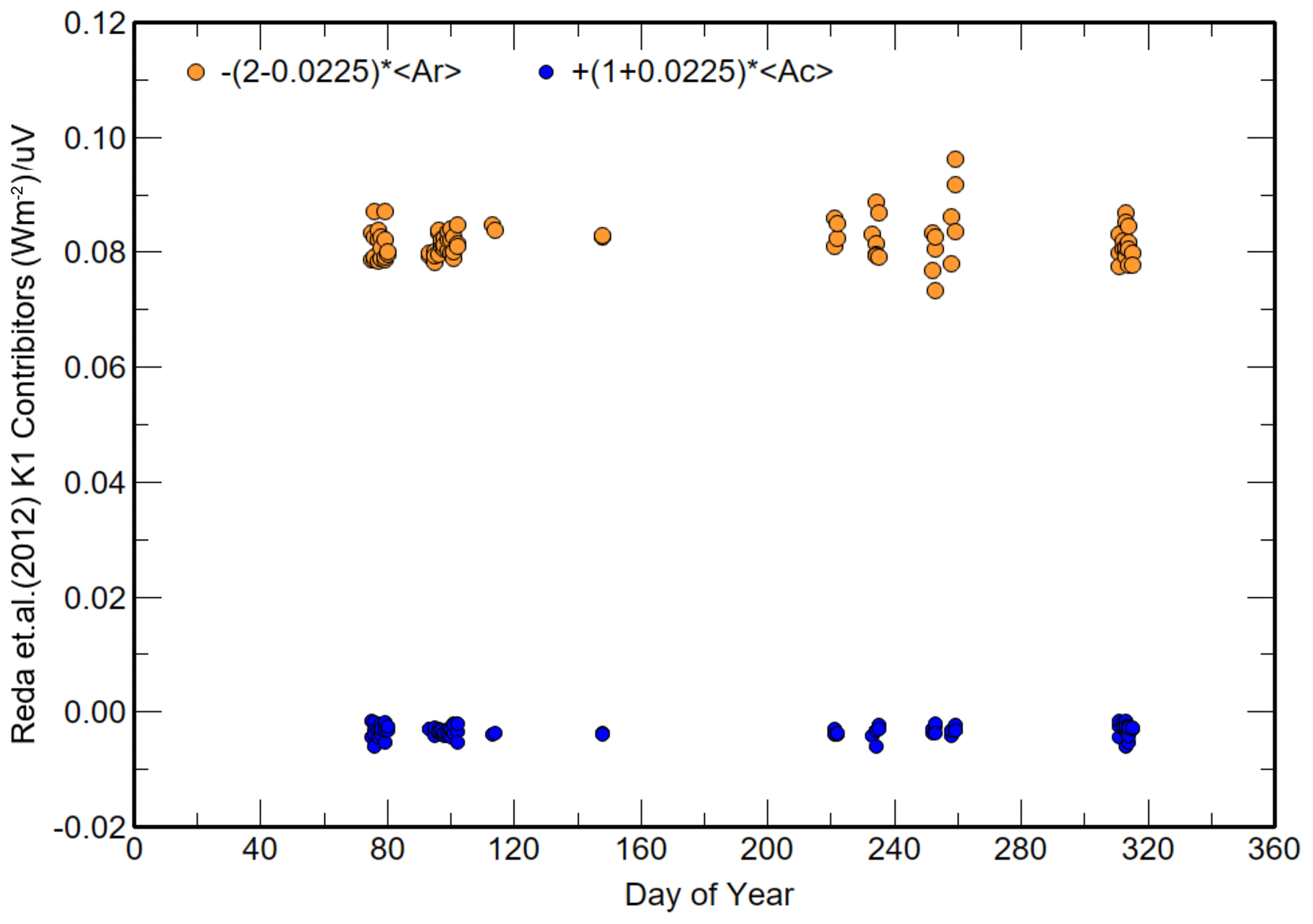
Figure 11 The two slope contributions to <K₁> for the equation developed by Reda et al. (2012).

The differences between the derived <C> for both the new and Reda et al. (2012) equations by linear LSQ are shown in Fig. 12 and for <W_atm> in Fig. 13. The different types of <C> are separated by about 2.5 µV (W⁻¹ m²), with the Reda et al. (2012) values being higher. The <W_atm> differences between IRIS4 and the Reda et al. (2012) equation were between ±12 Wm⁻², while the differences to the new equation are bounded by +4 and −8 Wm⁻², about half the range of the Reda et al. (2012) equation results.

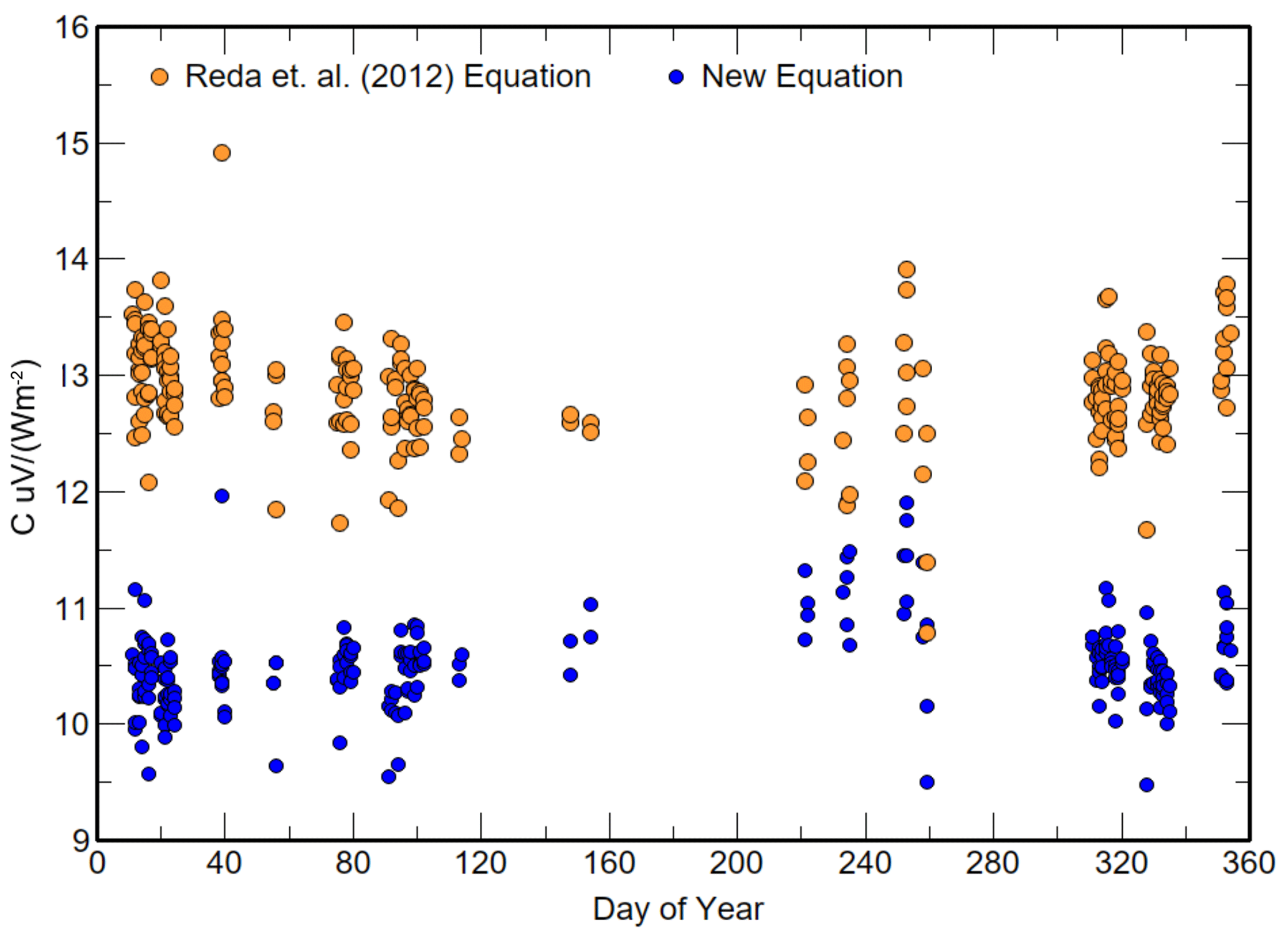
Figure 12 The derived C values derived from 244 linear LSQ calibrations in 2020 for the Reda et al. (2012) and new equations using a concentrator emissivity of 0.0225 for both and a convection coefficient of 6.5 for the new equation.

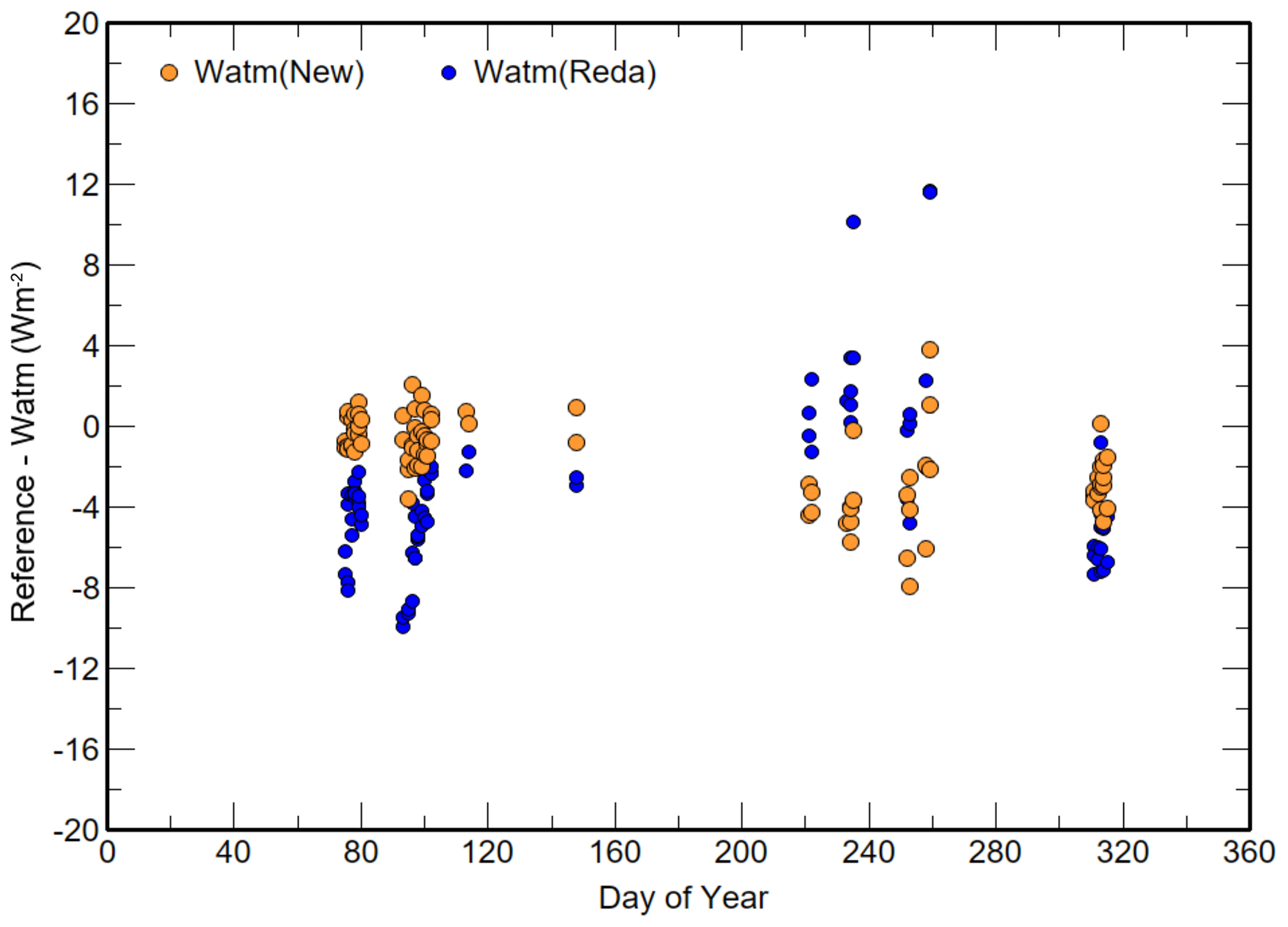
Figure 13 The comparison of <W_atm> derived from the new and Reda et al. (2012) equations to the mean IRIS4 irradiances for each linear LSQ calibration period in 2020.

9.3 Uncertainties in concentrator emissivity and convection coefficient

Three coefficients related to the concentrator are required for Eq. (18) to derive ambient irradiances and use the LSQ method of calibration. Zeng et al. (2010) provided a laboratory method for determining the transmission and an estimate of its uncertainty, but laboratory determinations of the emissivity and convection coefficient have not occurred.

The W_atm uncertainty estimates in Table 1 indicate that the incorrect assignment of the convection coefficient γ has a minor contribution to the calculation of W_atm even if the coefficient's standard uncertainty is 25 % from the true value. However, the emissivity is the second-largest contributor to uncertainty after the thermopile calibration coefficient in the determination of W_atm.

Table 8 provides an assessment of the uncertainty of the derived components of the linear LSQ method for the new equation. For this analysis, the uncertainties of the voltage signals are simply the estimate of the signal resolution, and the derived calibration constant incorporates any proportional uncertainty into the true voltage. The uncertainties of the receiver and concentrator irradiance are incorporated into LSQ slope and intercept statistics, as are the uncertainties of the differences between the receiver and the assumed air temperature.

In Table 1 the uncertainty of the convection coefficient was 1.5, but in Table 8 it is 0.3. Even after reducing the uncertainty component for the convection coefficient by a factor of 5 from that used in Table 1, this coefficient is the dominant contribution to the standard uncertainty of the derived <K₁> and is close to the dominant uncertainty contribution from the receiver irradiance <B_r> for the estimate of <τW_atm>.

The convection coefficient of air is dependent on the design of the air flow path and temperature, with a higher water vapour content also giving a higher coefficient. Empirical models of convection for the ACP are yet to be developed to determine the non-dimensional Nusslet parameter necessary for assigning and estimating the convection coefficient.

The new equation was developed by applying Kirchhoff's law of radiative transfer for radiative transfer in air. For the solar calibration method and the calibration using a reference irradiance, the ACP is essentially in steady state, while in the linear LSQ method the ACP is in a transient mode. Kirchhoff's law only applies in periods of radiative equilibrium, and this must be considered when modifying the cooling and heating cycle for linear LSQ calibrations.

Table 8 The standard uncertainty calculation for <K₁>, <τW_atm> and <W_atm> by linear LSQ regression of Eq. (18). The units of the slope components (<A_x>) are Wm⁻² µV⁻¹, while the intercept components are Wm⁻².

9.4 Future work

While the investigations above demonstrate that the new equation can be used with an ACP for terrestrial irradiance measurements and give good agreement with pyrgeometers with traceability to SI, there are still uncertainties related to the new equation and the characteristics of ACPs to be suitable direct references to SI irradiances. For example, a significant issue is how the Reda et al. (2012) equation and the new Eq. (18) can produce valid terrestrial irradiances but utilise thermopile sensitivities that differ by 25 % or more.

While the uncertainty in the convection coefficient has little impact on calculating outdoor irradiances, it is the dominant uncertainty when using the linear LSQ method for calibration with the new equation. The following are future actions recommended to increase the confidence of ACPs in acting as a primary reference to SI: a method for determining the convection coefficient, determining theoretical approximations of the ACP convection coefficient by developing an appropriate dimensionless Nusslet coefficient for the thermal and air flow characteristics of an ACP, determining whether the ACP can be calibrated in a black body but with a different process to that used with domed pyrgeometers, higher-frequency measurements in cooling and heating cycles to conform to the time offset between the thermopile reacting to a temperature change in the ACP base temperature, investigating whether the heating part of the LSQ data collection process can be used for LSQ analyses, and performing solar calibrations of the thermopile to determine an ACP's maximum possible thermopile responsivity.

10 Conclusions

The new equation for an ACP derived from the application of Kirchhoff's law and inclusion of a convection term provided irradiances that agreed with measurements from two reference IR radiometers over 11 months in 2020 assuming either a solar-derived calibration or a minimisation method.

The linear LSQ method of Reda et al. (2012) was modified for use with a new equation and developed so that the impact of individual contributors to the linear LSQ process could be assessed. As the only LSQ predictor was the thermopile voltage, the method allowed determination of five linear components independently of the Reda et al. (2012) and new equations. This also provided an estimate of the relative contribution of each component to the calibration values and their uncertainty contribution.

The linear LSQ results indicated that the new equation irradiances were for most cases consistent with the two reference radiometer irradiances but that consistency was dependent on the value of the convection coefficient. A method of examining the convection coefficient independently of a reference irradiance was developed by solving for τW_atm during the cooling and heating periods and highlighted the ∼9 s time lag between the representative voltage for the body and concentrator temperature measurements. When the lag was incorporated into the linear LSQ method, the confidence intervals for all slope quantities improved significantly, and systematic variations in the derived irradiance during a heating and cooling period were reduced but not eliminated. However, a process to determine the convection coefficient independently of outdoor or laboratory measurements has yet to be developed.

Via the linear LSQ method, an estimate for the concentrator transmission can also be obtained using a reference terrestrial irradiance. However, the preferred method should be laboratory measurements as performed by Zeng et al. (2010) but using the new equation rather than assuming that the measurements are performed in a vacuum.

A solar calibration of future ACP thermopiles is recommended provided the thermopile has not been subjected to solar irradiance for extended periods over several years. The solar calibration will produce an estimate of the thermopile responsivity that will be close to the maximum possible for the thermopile and thus provide either an independent estimate or a mechanism to assess the long-term stability of the ACP thermopile responsivity.