A modular field system for near-surface, vertical profiling of the atmospheric composition in harsh environments using cavity ring-down spectroscopy

Cavity ring-down spectroscopy (CRDS) has allowed for increasingly widespread, in situ observations of trace gases, including the stable isotopic composition of water vapor. However, gathering observations in harsh environments still poses challenges, particularly in regard to observing the small-scale exchanges taking place between the surface and atmosphere. It is especially important to resolve the vertical structure of these processes. We have designed the ISE-CUBE system as a modular CRDS deployment system for profiling stable water isotopes in the surface layer, specifically the lowermost 2 m above the surface. We tested the system during a 2-week field campaign during February–March 2020 in Ny-Ålesund, Svalbard, Norway, with ambient temperatures down to −30 ^∘C. The system functioned suitably throughout the campaign, with field periods exhibiting only a marginal increase in isotopic measurement uncertainty (30 %) as compared to optimal laboratory operation. Over the 2 m profiling range, we have been able to measure and resolve gradients on the temporal and spatial scales needed in an Arctic environment.

1 Introduction

Understanding exchange processes between the atmosphere and surface is fundamental to constrain fluxes between reservoirs in the Earth system. There exist substantial knowledge gaps on these processes and their representation in models, especially at high latitudes and in other cold environments (Wahl et al., 2021; Ritter et al., 2016). Near-surface (<2 m) gradients of scalars can be strengthened significantly due to the stable stratification that often occurs in these regions (Jocher et al., 2012; Zeeman et al., 2015), which ultimately governs the fluxes of trace gases such as methane, carbon dioxide and water vapor. In cold regions in particular, where ice and snow are prevalent, the quantification of the evaporation and condensation flux of water vapor requires multi-height, in situ measurements. In this regard, the stable isotope composition of the water vapor is a valuable asset, as quantified by the heavy isotopologues, HD¹⁶O (D = deuterium, ²H) and H${}_{\mathrm{2}}^{\mathrm{18}}$O, as well as by the rarer H${}_{\mathrm{2}}^{\mathrm{17}}$O. Hereby, the relative abundances of the stable water isotopes (isotopologues; SWIs) impart information about phase changes and thus the exchange between different reservoirs of the hydrological cycle.

Laser spectroscopy has enabled the continuous, high-resolution observation of the SWI composition in ambient air (Galewsky et al., 2016). In cavity ring-down spectroscopy (CRDS), the sample is guided through a measurement cavity with highly precise pressure and temperature control while the decay of a laser pulse in the infrared is measured (Crosson et al., 2002; Gupta et al., 2009). Since the spectrometers are designed for setup in a laboratory and similarly controlled environments, the in situ measurement often relies on pre-existing infrastructure (Bonne et al., 2014; Galewsky et al., 2011) or tents (Steen-Larsen et al., 2013; Wahl et al., 2021).

At such pre-existing structures, water vapor isotopes are often continuously measured at one or several fixed-height inlets. Fixed-height inlets must balance the number of lines with the robustness of their sampled gradient. Due to variations on many timescales, the inlet may not be at a height of interest for a particular measurement. In addition, over cold regions, turbulence in the surface layer often vanishes for extended periods (Mahrt, 2014), giving diffusional exchange processes a larger role. Due to kinetic fractionation of the SWIs, diffusional processes are particularly relevant for interpreting the measured water isotope signals in terms of surface properties (Thurnherr et al., 2021). While fixed-height manifold systems are only partially able to resolve near-surface gradients, assessing the surface exchanges requires detailed profiling of the structure.

The characteristically dry ambient air in the high latitudes, and thus the low absolute moisture concentration, limits the analytical precision of SWI measurements. Wall effects on the tubing can potentially further degrade measurement quality (Massman and Ibrom, 2008). Therefore, short, heated inlet lines limit potential interactions between water vapor and the inner walls of tubing. The use of short inlet lines also promotes a faster response of the CRDS analyzer, allowing for finer resolution of ambient signal variations in time and space. Munksgaard et al. (2011, 2012) applied a pragmatic approach, whereby the analyzer and accompanying equipment were housed inside a single plastic chest (on the order of 1 m³ in size) to facilitate their shipboard study of seawater along the tropical northeastern Australian coast. Despite the advantage of flexibility and low interference with the environment, a similar approach has not yet been attempted for the measurement of water vapor isotopes in the cold environmental conditions typical for high-latitude winter.

Here, we present a modular, in situ profiling system, termed the ISE-CUBEs, that adequately protects the CRDS analyzer from the harsh Arctic environment during profiling of the near-surface layer. The ISE-CUBE system primarily consists of a stack of weatherproof plastic cases interconnected for ambient air sample transmission. These cases have a footprint of less than 1 m² and a total volume of less than 0.5 m³. Attachment of a profiling sample arm allows for the detailed measurement of surface layer profiles in a 2 m range above the surface. An additional expansion module allows for the collection of water vapor in a cold-trap system for later laboratory analysis, including H${}_{\mathrm{2}}^{\mathrm{17}}$O. After a detailed description of the design principle and construction of the system, we evaluate its performance and the data quality based on measurements from a 2-week field campaign at Ny-Ålesund, Svalbard, where the system encountered severe cold temperatures.

2 Measurement system design

The general aim of the ISE-CUBE system design was to enable ground-based, near-surface profiles of the vapor isotope composition. Installation and operation should be unaffected by weather conditions, particularly with regard to temperature and precipitation. The entire system should also induce minimal disturbance to the flow around the measurement site. Wall effects in the inlet should be minimized with short tubing lengths. Condensation needs to be prevented to avoid measurement artifacts from fractionation and smoothed signals from memory effects. The system should be able to accommodate a cryogenic trapping module to collect discrete vapor samples for subsequent laboratory analysis. Based on these requirements, we designed a modular system that, in its core, was based on waterproof plastic containers, enabling setup by a single operator. We first give an overview of the overall arrangement of the measurement system before describing each module in more detail.

2.1 Overall measurement system setup

The main body of the ISE-CUBE system consists of a stack of the two primary modules (analyzer and pump modules) in addition to the cold-trap expansion module; a list giving specifics of individual components can be found in Table A1 (more details on system composition and construction can be found in Sect. S2 of the Supplement). All three modules use the same plastic container (iM2875 Storm, Pelican Products Inc), allowing for stacking and fastening of the stack, with a footprint of 0.38 m² (see Fig. 1). Each of the three modules is constantly ventilated with a 40 m³ h⁻¹ centrifugal fan. A plastic canvas can be placed over the stack for additional weather protection.

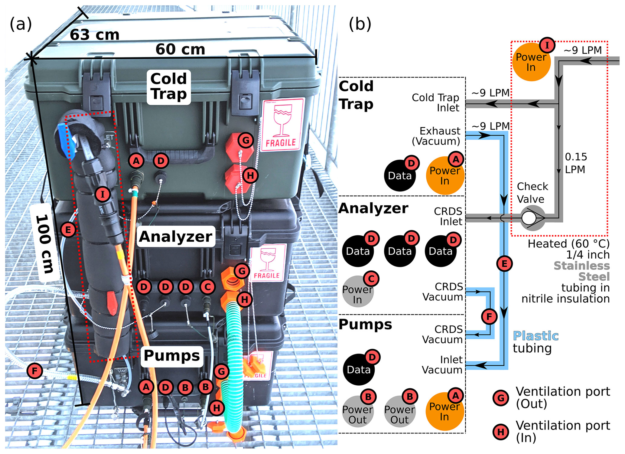
Figure 1 Overview of the ISE-CUBE system. (a) ISE-CUBEs in stacked configuration (from top to bottom): cold-trap expansion module, analyzer module, and pump module. (b) Flow diagram for the entire ISE-CUBE system, including flow rates and connectors. A heated inlet assembly (dotted red area in both) connects the three modules for common gas transmission. See text for details.

Gas transmission within the stack is via an inlet flow assembly (Fig. 1, dotted red area) composed of approximately 70 cm of $\mathrm{1}/\mathrm{4}$ in. stainless steel tubing (Swagelok Inc.), heated to 60 ^∘C with self-regulating heat trace cabling (Thermon Inc.). A main flow of approximately 9 L min⁻¹ (liters per minute) is drawn into the assembly (Fig. 1b), with most going through the cold-trapping module, using a vacuum pump in the pump module (Fig. 1b, “Inlet vacuum”). Analyzer flow is split off prior to entering the cold-trapping module. A one-way check valve (6L-CW4S4, Swagelok Inc.) upstream of the analyzer inlet bulkhead (Fig. 1b, “Check Valve”) prevents reversal of the flow of sample air bound for the analyzer. The external vacuum pump of the CRDS analyzer (N920AP.29.18, KNF DAC GmbH) is also located in the pump module (Fig. 1b, “CRDS vacuum”). The inlet flow assembly also allows for connection to additional lengths of inlet tubing, such as the profiling module, which enables sampling at adjustable heights (see Sect. 2.4). We will now describe all four modules of the measurement system individually, beginning with the analyzer and pump as the core modules.

2.2 Analyzer module

We use a Picarro CRDS water isotope analyzer (L2130-i, Picarro Inc., USA) as the central element of the analyzer module (Fig. 1, middle container). The analyzer module is lined with custom-fit low-density polyethylene (LDPE) foam padding to protect the analyzer. Some padding can be removed to increase ventilation flow for better temperature regulation, depending on ambient conditions during field operations. With a power draw of ∼100 W in steady state, there is substantial heating from the analyzer. Therefore, adequate ventilation is required to keep the analyzer internal temperatures below around 50 ^∘C, as prolonged exposure to higher temperatures (above 70 ^∘C) can permanently damage electrical components.

The analyzer computer can be controlled from an external laptop through an ethernet (RJ45) cable or via USB-connected monitor and keyboard–mouse combination, with the “data” connectors (Fig. 1, D). The particular analyzer used here (ser. no.: HIDS2254) is a custom modification of the standard L2130-i, which enables higher flow rates, similar to the analyzer described in Sodemann et al. (2017). The high flow rate is obtained by replacing the internal, constricting orifice (70 µm) needed for low-flow mode (typical flow rates 0.035 L min⁻¹) with a standard $\mathrm{1}/\mathrm{4}$ in. stainless steel section in addition to using a stronger vacuum pump (N920AP.29.18, KNF DAC GmbH, Germany). High flow rates (about 0.15 L min⁻¹) enable faster analyzer response and 4 Hz sampling, but they also cause more variable pressure inside the measurement cavity. The full impact of this particular configuration will be discussed in more detail below (Sect. 4.1). Sample air is guided from the exterior inlet bulkhead of the module into the analyzer via a 20 cm piece of flexible, $\mathrm{1}/\mathrm{4}$ in. polytetrafluoroethylene (PTFE) tubing. A similar length of $\mathrm{3}/\mathrm{8}$ in., wire-reinforced, PVC tubing (K7160-06, Kuriyama of America Inc.) connects the vacuum port of the analyzer to the exterior bulkhead (Fig. 1b, “CRDS Vacuum”). The vacuum and electrical bulkheads of the analyzer module then connect to the pump module (Fig. 1, F: vacuum, B and C: electrical).

2.3 Pump module

The pump module contains the pumps and additional components necessary for operation of the analyzer (Fig. 1, bottom container). The pump module is connected to the analyzer module with a $\mathrm{3}/\mathrm{8}$ in., wire-reinforced, PVC tube (K7160-06, Kuriyama of America Inc.), providing the vacuum necessary for the analyzer (Fig. 1b, “CRDS Vacuum”). The inlet vacuum pump (N022AN.18, KNF DAC GmbH, Germany) continuously flushes the inlet tubing, providing the main flow for both the analyzer and the cold-trapping module (see Sect. 2.5). Additionally, a small 300 W uninterruptible power supply (UPS; EL500FR, Eaton) inside the module protects the analyzer from possible power fluctuations and short power breaks. This UPS also provides 12 V power (via a 230 V AC-to-DC adaptor) for the profiling module (Fig. 1, B). All components in the pump module are strapped to an aluminum support frame, which itself is firmly wedged between the lid and bottom of the case, when the case is shut. Thereby, we could avoid drilling unnecessary mounting holes in the plastic case. Together, the analyzer module and the pump module are the two essential modules for in situ isotopic measurement of water vapor. We will next describe the profiling module, which enables high-resolution vertical profiling of the lowermost levels of the surface layer.

2.4 Profiling module

The profiling module allows us to measure near-surface gradients of water vapor (atmospheric composition, more generally), as well as to investigate the exchange processes between surface and atmosphere. The profiling module allows for the acquisition of vertical profiles of the ambient air at any height in a 2 m range (Fig. 2). The lean design is expected to cause minimal flow disturbance at the measurement site. The module attaches to the inlet assembly (Fig. 1, dotted red area) and consists of approximately 4 m of $\mathrm{1}/\mathrm{4}$ in. stainless steel tubing (Swagelok Inc.), heated to 60 ^∘C with self-regulating heat trace cable (Thermon Inc.) and surrounded with 2 cm thick foam nitrile insulation. Profiling capabilities are enabled by encasing the final 1.9 m of tubing in an aluminum articulating arm (Fig. 2). The base of this arm is then attached to an aluminum mast and tripod with a custom-made steel mount (see Supplement). The tripod serves as the frame for a winch and pulley system to manually control the sampling height (Fig. 2). Additional environmental parameters are acquired during profiling from a sensor package mounted on the “head” of the arm, near the air inlet. The height of the inlet is monitored by ultrasonic distance sensors (HC-SR04, SparkFun Electronics; Fig. 2, red box). Air temperature at inlet sampling height is measured using a temperature probe (VMA324, Velleman; blue rectangle in Fig. 2b). Both variables are logged onto an SD card via a microcontroller (UNO, Arduino) housed inside a weatherproof container (Fig. 2a, yellow case at lower left).

Figure 2 The profiling module, with articulating arm. (a) Profiling module during field deployment. The inlet “head” can be seen in upper right of photo, with ultrasonic distance sensors encased in red plastic housing. The temperature sensor (not visible) is located on opposite side of the “head”. The black winch in bottom left of the photo controls the inlet height via a pulley system. Also visible in the bottom left is the yellow case containing the power supply and data logger for temperature and distance sensors. Black tubing leading off to the left connects to ISE-CUBE inlet. (b) Dimensional diagram for articulating arm.

An alternate deployment frame was also custom-made for the profiling arm (Fig. S1 in the Supplement). This allowed us to mount the arm on an elevated platform and to reach downwards to the surface of the water (such as at the Fjord deployment site, Sect. 3.1). The arm mounts onto a ladder-like construction with steel U-bolts. Two right-triangular steel supports are mounted on their base legs, perpendicular to the face of the ladder, forming the main structure of the frame. Base and height legs of the triangular supports are approximately 1 m long. A wheel-and-axle crossbeam connects the two supports at the upper point of the height leg; this crossbeam supports the steel cable moving the arm. Any rung of the ladder construction can slide into two steel brackets which are bolted to the platform. While in “normal” orientation, the ladder construction and the head of the inlet arm would be horizontal. However, the entire frame could then tip forwards, pivoting about the secured rung, with the ladder and inlet head both ending up vertical. This allowed us to make measurements 1.0 to 1.5 m further down at the Fjord site, though this did require an additional front-facing ultrasonic sensor. The fine-scale adjustment of the inlet head height was still possible with the winch and cable system and was necessary to account for the tidal height changes of the seawater.

2.5 Cold-trapping expansion module

We included a cold-trap module in the ISE-CUBE system, providing the ability to retrieve sample material from the field for subsequent laboratory analysis. This laboratory analysis could also include δ¹⁷O for calculation of the ¹⁷O-excess. Many commercially available cold-trapping options involve the use of liquid cooling agents, such as ethanol or isopropyl alcohol. Peters and Yakir (2010) demonstrated the feasibility of collecting vapor samples with a Stirling cycle cryocooler as the cryogenic source of a cold trap. Due to the safe transportation and fast installation of such a cold trap, we adopted the basic design of Peters and Yakir (2010) for the ISE-CUBE cold-trap expansion module.

The cryocooler migrates heat away from the tip of a cryogenic “finger” towards the body of the cryocooler, where the heat is radiated away through a radiator fin. By attaching this cryogenic finger to a thermally conducting mass (150 g of brass and aluminum) encircling a glass sampling vial, it directly cools the vial down to −80 ^∘C. Incoming water vapor in sample air (Fig. 3b, “Inlet”) is routed through a combination of $\mathrm{3}/\mathrm{8}$ in. stainless steel tubing and connectors and is then introduced to the cooled glass collection vial connected to the large bore tubing with a custom-made polycarbonate adapter (“PC” in Fig. 3b). Upon entering the vial, the water vapor is rapidly cooled below its frost point, and it collects on the interior walls of the glass vial. The dried air exits the glass vial via a $\mathrm{1}/\mathrm{8}$ in. length of stainless steel tubing, leading out of the end of the $\mathrm{3}/\mathrm{8}$ in. tubing–connector combination. Finally, this $\mathrm{1}/\mathrm{8}$ in. tubing is connected to the inlet vacuum pump (Figs. 1b and 3b, “Exhaust (Vacuum)”), which provides the necessary flow for the cold trap. After the sampling period is complete, the flow is shut off with the needle valve (Fig. 3, D), and the vial is manually removed, sealed and stored until laboratory analysis, which can be done from the same vial. Also, the relatively small size of the setup easily fits within the standard ISE-CUBE container (Fig. 1, top box).

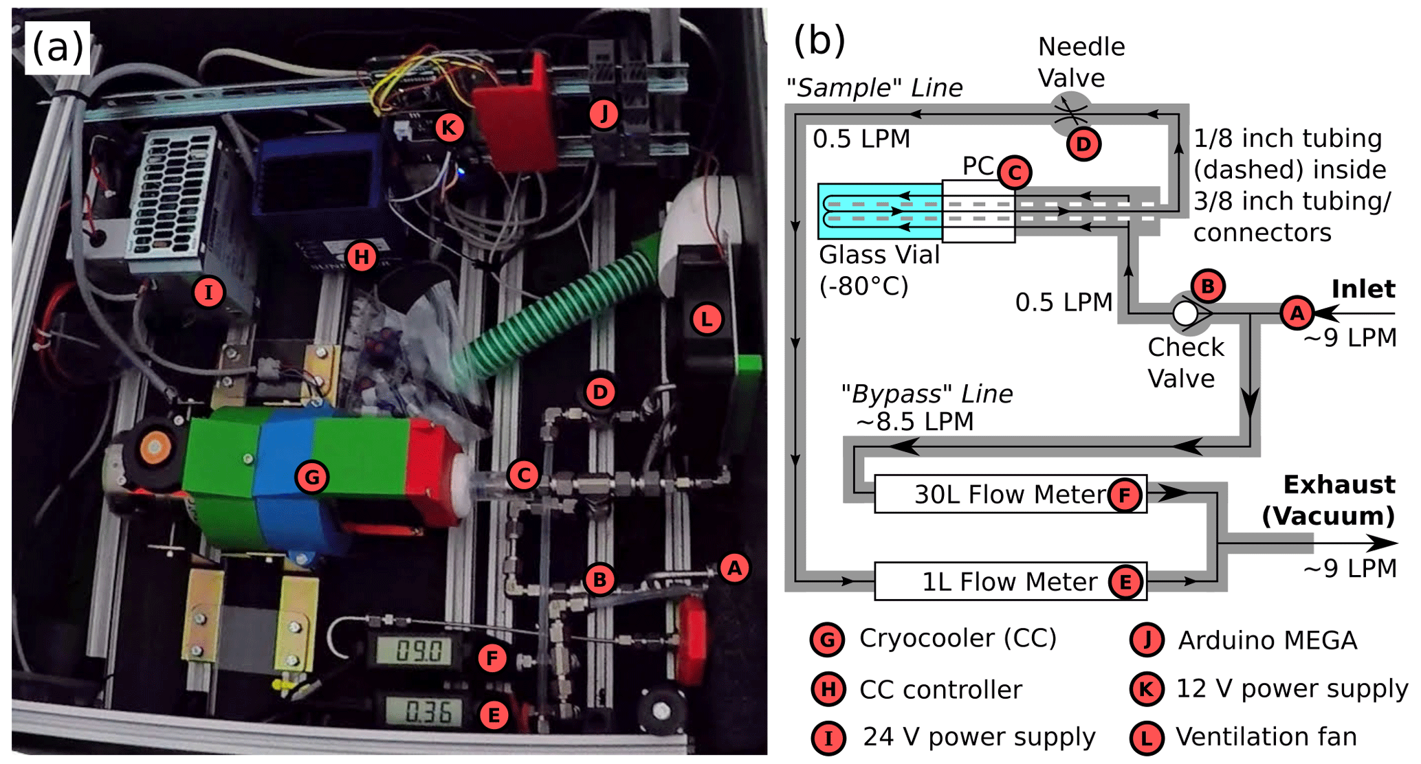
Figure 3 The cold-trapping module. (a) Interior of the module; cryocooler is surrounded by green, blue and red plastic near photo center (“G”). (b) Flow diagram for the module. “PC” indicates placement of polycarbonate vial adapter. See text for details.

We modified the original design of Peters and Yakir (2010) with regard to two aspects, namely the choice of cryocooler and the flow configuration. Firstly, we opted for a more powerful cryocooler (Leon Peters, personal communication, 20 March 2019), enabling faster and more consistent cooling of the sampling vial. Our chosen cryocooler (CryoTel MT, Sunpower Inc.; Fig. 3, G) takes 5 to 6 min to reach −80 ^∘C, at which temperature it has 23 W of cooling power. Secondly, as the system was designed to work in concert with the analyzer and pump modules, we utilized the inlet pump described in Sect. 2.3 to provide flow through the collection vial. Accomplishing this required the splitting of flow inside the cold-trapping module into a “sample” and “bypass” line (Fig. 3b). The sample line allowed incoming, moist air into the glass collection vial, with flow regulation (approximately 0.5 L min⁻¹ or less) via a manual needle valve. The bypass line carried the excess flow (approximately 8.5 L min⁻¹), ensuring that the flushing of the inlet was maintained. Flow rates through the sample and bypass lines were monitored using 1 and 30 L min⁻¹ mass flow meters (TopTrak 822, Sierra Instruments Inc.; Fig. 3, E and F), respectively. These flow meters recorded onto an SD card via microcontroller (Mega, Arduino; Fig. 3, K), which in turn allowed for remote monitoring of the flow rates via the external USB bulkhead (Fig. 1, D). Splitting the lines in such a way allowed the inlet pump to provide flow through both the cold-trap collection vial and the inlet tubing.

3 Performance test datasets

3.1 Campaign site and weather conditions

The performance of the ISE-CUBE system was evaluated based on a field campaign dataset obtained in challenging Arctic measurement conditions at the scientific settlement of Ny-Ålesund, Svalbard (Fig. S2), during the ISLAS2020 campaign. The principal aim of the ISLAS2020 field experiment was to obtain detailed in situ measurements of isotope fractionation in an Arctic environment, characterized by open fjord water and snow surface. Ny-Ålesund, with the adjacent strong air–sea interaction in the Fram Strait, is a well-suited location to make such observations. In particular, during winter and spring, this region is frequently subject to periods of strong marine cold-air outbreaks, associated with intense evaporation (Papritz and Spengler, 2017).

In Ny-Ålesund, we deployed at two measurement sites, the first being approximately 300 m south of Ny-Ålesund, on the tundra (78.92117^∘ N, 11.91361^∘ E). This site was also referred to as the “snow” location and was used from 25–28 February 2020. The second site was located on a concrete pier at the northernmost edge of the settlement (referred to as “Fjord”; 78.92873^∘ N, 11.93552^∘ E) and was used from 7–14 March 2020. The profiling module utilized the tripod frame while at the Snow site, while it used the tipping frame at the Fjord site, to reach further down towards the surface of the water.

General 2 m air temperature and 10 m wind speed and gust information for the Ny-Ålesund weather station (SN99910) were retrieved from the Norsk Klimaservicesenter (https://seklima.met.no/observations, last access: 3 February 2021). From this station dataset, 20-year climatological conditions were established by considering the hourly dataset of the period between 21 February and 14 March, between 2000 and 2019. The time period from 21 February to 14 March in Ny-Ålesund has a climatological median air temperature for 2000–2019 of −12 ^∘C, with 50 % of hourly average temperatures being between −16 and −6 ^∘C (Fig. 4, black). In comparison, the majority of the ISLAS2020 campaign was spent in temperatures spanning −26 to −18 ^∘C, with a median value of −20 ^∘C (Fig. 4, blue). The coldest temperatures experienced during the campaign (−30 ^∘C) were comparable to the minimum temperature in the 2000–2019 climatology, which was −32.5 ^∘C (Fig. 4, dashed black line). Additionally, Dahlke et al. (2022) have identified February and March 2020 as having some of the strongest marine cold-air outbreaks of the last 42 years. Overall, with several episodes of extreme cold, our deployment was a formidable testing ground for the system.

.

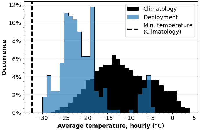
Figure 4 Histogram of hourly average temperatures in Ny-Ålesund for 2000–2019, 21 February to 14 March (“Climatology”, black) alongside the same from during the ISLAS2020 field campaign (“Deployment”, blue). Dashed black line denotes minimum hourly temperature from the 2000–2019 period. Data from Norsk Klimaservicesenter, Ny-Ålesund (SN99910)

3.2 Data processing

The ISE-CUBEs produce two main data streams pertaining to the analyzer and profiling modules, with each module internally recording its own respective stream. The cold-trap expansion module does a similar task for its own data stream. An overview of the information contained in these data streams is given in Table 1. The isotopic data stream generated by the analyzer in the analyzer module is the primary dataset and also has the highest sampling frequency of 4 Hz. The primary environmental parameters observed by the analyzer are humidity (volumetric mixing ratio), δ¹⁸O and δD, alongside a multitude of analyzer diagnostic metrics, including temperature and pressure internal components. Before further use, the isotope dataset was calibrated and corrected as described in Sect. 3.3 below.

Table 1 Parameters logged by the ISE-CUBE system.

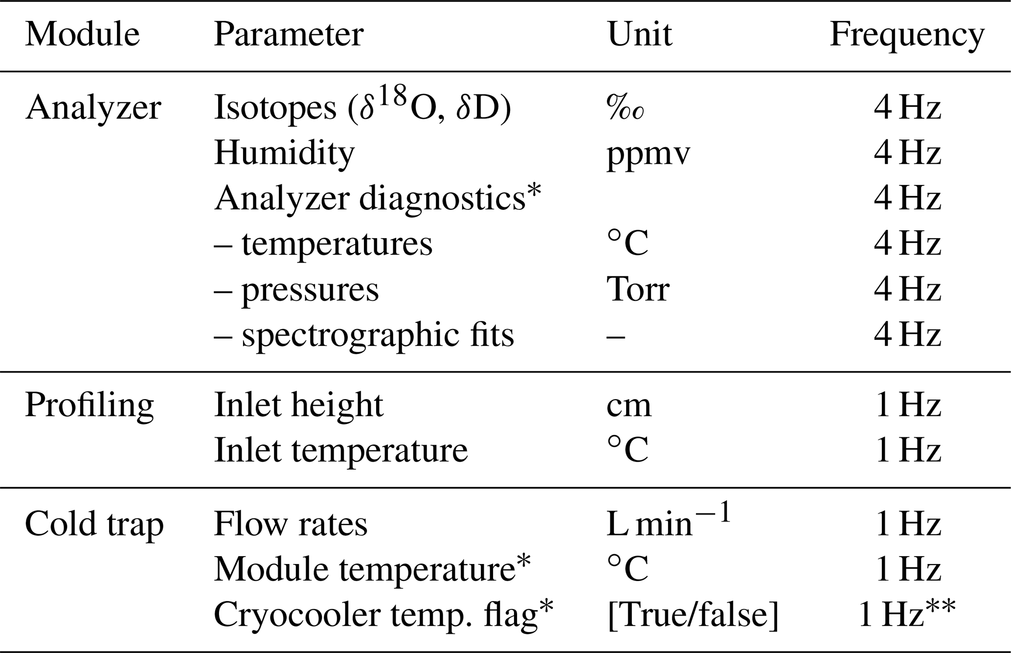
^* indicates parameters classified as metadata, providing information on the quality of the data collected. ${}^{**}$ While flow rates and metadata of the cold-trap module are recorded as 1 Hz, sample collection times varied.

Both the profiling and cold-trap modules measure at 1 Hz via Arduino microprocessors and record parameters to SD cards. The profiling module records the temperature at the inlet head in addition to height distances measured by the ultrasonic sensors. Laboratory calibration of the temperature probe showed a systematic offset of +0.67 K, which is accounted for during post-processing. The cold-trap expansion module monitors and records the flow through the collection vial alongside the remaining flow through the “bypass” line, as well as the temperature inside the module container. The same module also flags whether the cryogenic finger is within 5 K of the target temperature (−80 ^∘C). Throughout the campaign, all module timestamps were compared to universal coordinated time, with offsets accounted for and datasets synchronized during processing.

The analysis of module performance that will follow in Sect. 4 makes use of datasets averaged across multiple time intervals. The technical analysis of analyzer module performance in Sect. 4.1 and 4.2 uses a 1 s averaged dataset, as does the assessment of the profiling-module sensors in Sect. 4.3. However, subsequent evaluation of the profiling module in regards to sample transmission uses the native 4 Hz resolution. Based on our system characterizations evaluated below, our final calibrated isotopic-profiling dataset is averaged over 30 s (Sect. 4.4 and 4.5).

3.3 Isotope calibration and data processing

Requisite calibrations of the analyzer were performed immediately preceding and following deployment at each measurement site, at Kings Bay Marine Laboratory in Ny-Ålesund. Isotopic measurements are calibrated on the VSMOW2-SLAP2 (Vienna Standard Mean Ocean Water 2 – Standard Light Antarctic Precipitation 2) scale, composed of international, primary standards. The use of the scale allows for the relative ratios of heavy to light isotopes (R_sample) measured in CRDS analyzers to be normalized to a standard (R_standard), as described in Eq. (1) (Craig, 1961):

$$\begin{array}{}\text{(1)}& {\mathit{\delta }}^i=\left({\displaystyle \frac{R_{\mathrm{sample}}^i}{R_{\mathrm{standard}}^i}}-\mathrm{1}\right)\cdot \mathrm{1000}\left(\mathrm{‰}\right).\end{array}$$

The value of the resulting δⁱ (with i representing one of the heavy SWIs) is expressed in per mil (per thousand, ‰). For our calibrations, we employed two secondary standards, whose isotopic values on the VSMOW2-SLAP2 scale have been established in the laboratory. The two secondary standards used were DI (δ¹⁸O: $-\mathrm{7.68}\pm \mathrm{0.07}$ ‰ and δD: $-\mathrm{49.7}\pm \mathrm{0.4}$ ‰) and GSM1 (δ¹⁸O: $-\mathrm{32.90}\pm \mathrm{0.05}$ ‰ and δD: $-\mathrm{261.6}\pm \mathrm{0.3}$ ‰). Liquid standards were delivered with the Standards Delivery Module (SDM) device (A0101, Picarro Inc.), utilizing a Drierite-filled moisture trap as a source of dry air. Only sufficiently stable calibration signals lasting longer than 10 min are considered for use in calibrating the dataset. As the specific humidity at the deployment site can be well below 3.5 g kg⁻¹ for the time of year, a correction of the isotope composition was applied during post-processing according to the quantified mixing ratio–isotope ratio dependency by Weng et al. (2020), specific to the analyzer used in the field. Several calibrations made during the ISLAS2020 field deployment were between mixing ratios of 3.5 and 0.5 g kg⁻¹ and confirm overall agreement with the mixing ratio–isotope ratio dependency determined in the laboratory.

Calibrations performed in the Kings Bay Marine Laboratory were considered valid only if they passed automatic quality control thresholds, such as humidity variation below 0.3 g kg⁻¹ (500 ppmv). Across 17 valid calibrations, DI measurements had a standard deviation of 0.15 ‰ for δ¹⁸O and 0.48 ‰ for δD. For both isotope species, this standard deviation is similar to (or smaller than) the standard deviation typical during any individual calibration. Total measurement drift across the campaign duration for DI was found to be smaller than these standard deviations. The GSM1 standard experienced technical issues with the SDM during multiple calibrations. The standard deviation across the 17 valid calibrations for this standard was 0.18 ‰ (δ¹⁸O) and 0.47 ‰ (δD), again of a similar magnitude to the variabilities seen in individual calibrations. As for DI, the total measurement drift across the campaign duration for GSM1 was found to be similar to or smaller than these standard deviations. Overall, these drift values are compatible with the behavior exhibited by the same analyzer during previous use in the lab and field (Weng et al., 2020; Chazette et al., 2021) and exceed the manufacturer's typical performance specifications (Picarro Inc., 2021).

3.4 Analyzer performance benchmark periods

We introduce two reference periods for comparison to our analyzer's behavior in the field. The first represents the optimal operating environment for the analyzer, a well-controlled laboratory setting with ambient room temperatures of approximately 20 ^∘C. This first period runs from June–July 2020 when the same analyzer was used at FARLAB, University of Bergen, Norway. During this time, the analyzer was routinely sampling standard vapor with mixing ratios down to 0.155 g kg⁻¹, comparable to humidity minimums encountered in the field. The second period more closely resembles a typical deployment, with the instrument sampling exterior air through an inlet tube while installed inside a building with a controlled environment, but is less stringently regulated than a university research laboratory. During this short-term deployment, the same analyzer was installed at the Zeppelin mountain observatory (475 m a.s.l.), 2 km SSW of Ny-Ålesund. The installation spanned from 29 February 2020 to 2 March 2020, with the analyzer measuring outside the ISE-CUBE module. Both reference periods sampled at 1 Hz and at a lower flow rate than we used in the field. Across the three environments, we compare the overall analyzer temperature; the cavity temperature and pressure; and the temperature of the “warm box”, an enclosure housing essential analyzer electronics critical for spectroscopic fitting.

3.5 Additional datasets

Since 2010, the Alfred Wegener Institute (AWI) has operated the Ny-Ålesund eddy covariance (EC) site (Jocher et al., 2012; Schulz, 2017), about 300 m south of the settlement and approximately 20 m away from the ISE-CUBE system during the initial deployment phase at Snow. This EC station measures, amongst others, air temperature at 1.0 m, averaged over 30 s. Temperatures are measured by a Thies Clima compact temperature sensor (2.1280.00.160, Adolf Thies GmbH & Co. KG, Germany) inside a ventilated shield (1.1025.55.100, Adolf Thies GmbH & Co. KG, Germany). This temperature was used for field validation of the temperature probe fixed to the head of the profiling module, as described in Appendix C.

4 Results

We now detail how the field conditions influenced analyzer performance and thus data quality, using the laboratory and observatory periods as performance benchmarks. Thereby, we focus first on temperature and pressure conditions of the analyzer (Sect. 4.1) before evaluating the impact of field conditions on the water isotope measurements (Sect. 4.2). Then we detail the performance of the profiling module, especially the capability of the module to deliver samples to the analyzer for the purpose of resolving vertical profiles (Sect. 4.3). Finally, the performance of the cold-trap expansion module is briefly presented (Sect. 4.4).

4.1 CRDS analyzer response to ambient conditions

Using our laboratory and observatory benchmarks, we now detail how the field conditions influenced analyzer performance and thus data quality. We first use the data acquisition system (DAS) temperature (T_DAS) measured inside the analyzer housing as a proxy of the overall temperature and condition of the analyzer (Picarro Inc., 2013). Then, we characterize the measurement cavity through its temperature (T_C) and pressure (p_C). Finally, we study essential analyzer electronics, namely the wavelength monitor (WLM), via the warm-box temperature (T_WB).

4.1.1 Overall analyzer temperature

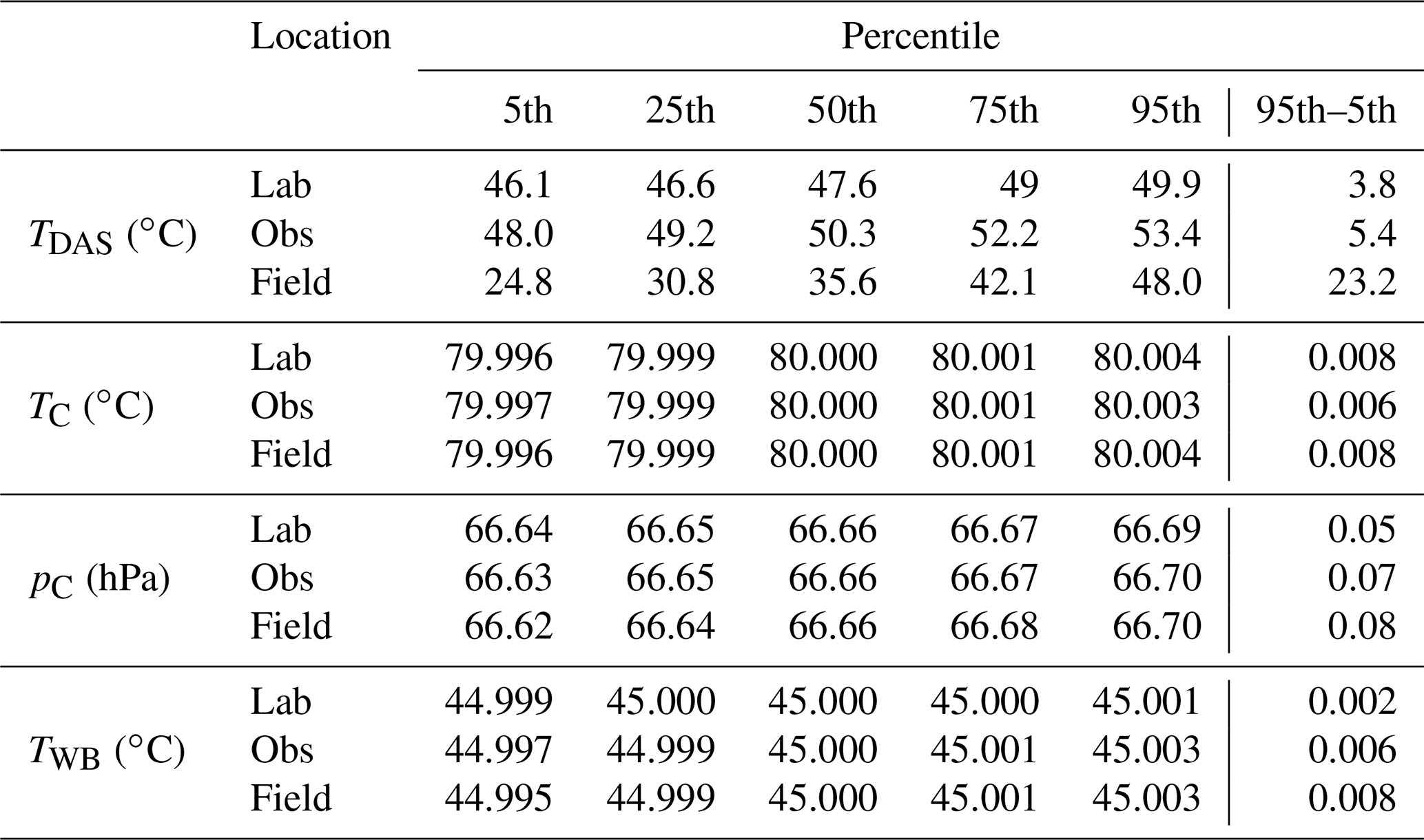
The T_DAS serves as a first-order proxy for the overall measurement environment of the analyzer. As the T_DAS results from a balance between radiant, excess heat from other components (especially from the measurement cavity) and constant ventilation with ambient air, its value can span a wide range. In the laboratory, T_DAS values are typically within a narrow distribution, with 94.3 % of T_DAS falling within 45 to 50 ^∘C (Fig. 5a, black). This narrow distribution is similar for the observatory (91.7 % within 47.5 to 52.5 ^∘C). In contrast, the most frequent T_DAS from the field is within the 30 to 32.5 ^∘C range (17.3 %; Fig. 5a, blue bars). Across all percentiles (Table 2), the T_DAS in the field is lower and more broadly distributed. Thus, the overall temperature of the analyzer was colder and more variable in the field as compared to the lab. However, the T_DAS stayed within its necessary range for operation, with the analyzer remaining functional for the entirety of the two deployments. Therefore, any further impacts from this increased variability require exploration. We now continue our investigation with the conditions in the measurement cavity, the most critical element of the analyzer.

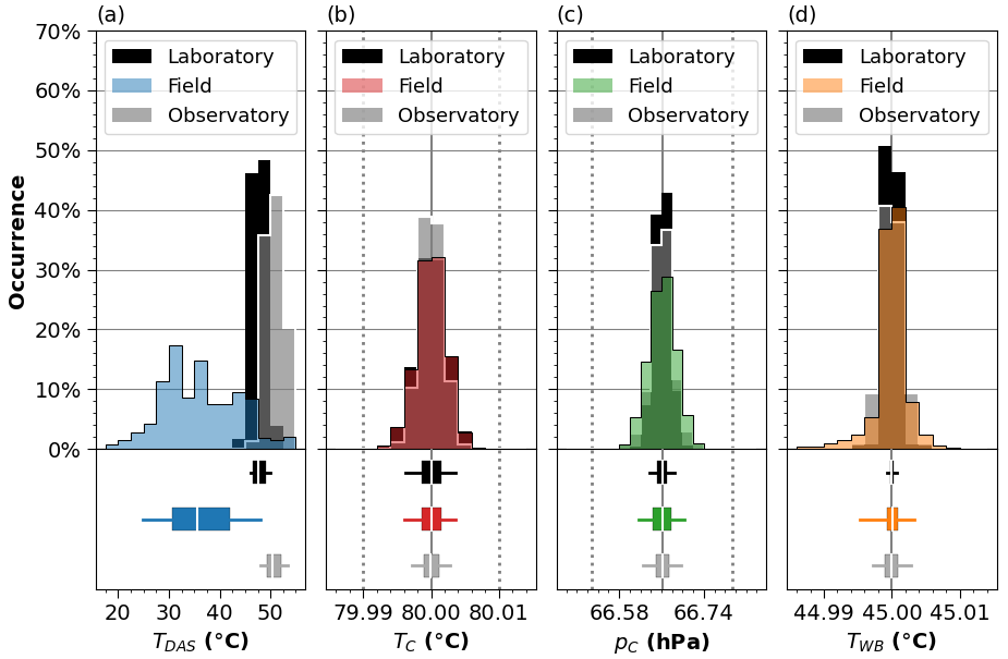
Figure 5 Relative occurrence of (a) DAS temperatures, T_DAS (2.5 ^∘C bins); (b) cavity temperatures, T_C (0.002 ^∘C bins), (c) cavity pressures, p_C (0.02 hPa ins); and (d) warm-box temperatures, T_WB (0.002 ^∘C bins) during CRDS operation, for field deployment periods (colored) as compared to reference periods, laboratory (black) and observatory (gray). Lower panels show total distributions for the three periods in boxplot form, with the median (white line), interquartile range (IQR; box limits), and 95th and 5th percentiles (whiskers). Solid vertical lines for panels (b), (c) and (d) indicate parameter target value. Dotted lines for panels (b) and (c) indicate instrument control precision as per manufacturer. Note that “Field” and “Laboratory” overlap closely in panel (b).

Table 2 Analyzer statistics for the overall analyzer temperature (T_DAS), the cavity temperature and pressure (T_C and p_C), and the warm-box temperature (T_WB). Percentile intervals as indicated from field, laboratory and observatory periods. Corresponding 95th to 5th span provided for the same.

4.1.2 Cavity temperature and pressure

The precision and accuracy of the temperature inside the measurement cavity of the analyzer are of the utmost importance for precise spectroscopic measurements. For this reason, the analyzer regulates the cavity temperature very precisely at about 80.00±0.01 ^∘C (Steig et al., 2014). The median T_C is identical across the field, laboratory and observatory periods, 80.000 ^∘C (Fig. 5b and Table 2). Between the 95th and 5th percentiles, T_C distributions between field and laboratory are indistinguishable from one another. In the field, the cavity temperature stays within this range for 99.99 % of the time, which exceeds the laboratory benchmark (99.97 %). Finally, there exists no correlation between T_C and T_DAS while deployed in the field. Therefore, 99.99 % of field observations are made with cavity temperatures within specified limits and are indistinguishable from the laboratory benchmark.

The pressure inside the cavity must be maintained at 66.66±0.10 hPa (Steig et al., 2014). The ISE-CUBE system does little to modify the native flow pattern of the analyzer; therefore, we expect that the p_C exhibits no dependence on the DAS temperature. Just as with T_C, there is no correlation between p_C and T_DAS while deployed in the field. Overall, the specified range is maintained for 99.95 % of the field deployment, which differs from our laboratory benchmark (99.99 %). Indeed, both the laboratory and observatory reference periods have slightly narrower distributions (Fig. 5c and Table 2). So even though the cavity pressure remained within limits for the vast majority of the time, some aspect of the field deployment had an impact on cavity variability. After further investigation into other potential differences between the laboratory and field setups, we determined that this difference in cavity pressure variability stems from the enhanced sample flow configuration of the analyzer while being used in the field (Sect. 2.2) and is not inherent to a specific aspect of the ISE-CUBE system. The fast-response configuration on this instrument has been used in a previous field deployment (Chazette et al., 2021) and is within the scope of the standard operating procedures.

In summary, the accuracy and precision of cavity pressure and temperature remained within necessary limits and were comparable with our two benchmark periods. In particular, the cavity temperatures were indistinguishable between laboratory and field. We therefore expect the measurement cavity to have been functioning reliably during the field deployment. As a final analyzer parameter, we now investigate the warm-box temperature.

4.1.3 Warm-box temperature

The WLM is part of the analyzer's laser control loop and is continuously used to target the desired wavelengths, reducing instrument drift (Crosson, 2008; Gupta et al., 2009). It is contained within the warm box; the interior temperature of the warm box is regulated by the analyzer to 45 ^∘C. In our laboratory benchmark, 90 % of the variation about this target was within 0.002 ^∘C (Table 2). In comparison, the same range of T_WB in the field has 4 times the variability (Table 2). The field distribution is more similar to our observatory benchmark period (Fig. 5d and Table 2). Even when compared to this benchmark, T_WB from the field has a tendency towards lower temperatures (Fig. 5d). This indicates that the temperature inside the warm box is coupled to the changing (usually cooling) analyzer temperature. Since the analyzer has a gas inlet at the back, leading to the WLM, ambient air temperature could also more directly impact the T_WB than other components. As an example, sudden dips and spikes in T_WB correspond with the onset of drops and rises in T_DAS (Fig. S3). As this range of variations could potentially have an impact on measurement quality, we now assess WLM performance in more detail during lab and benchmark periods.

For the evaluation of the WLM performance, we use three spectroscopy metrics that quantify the difference between an expected model spectrum versus the fitted-absorption spectrum that is actually measured by the analyzer (Johnson and Rella, 2017). The baseline shift (BS) describes the absolute value change of the spectral baseline; the slope shift (SS) indicates the change in the slope of the baseline (Johnson and Rella, 2017; Weng et al., 2020); and the residual (RS) represents the residual errors present in the fit spectrum compared to the expected spectrum. The spectra have a first-order dependency on mixing ratio with resulting baseline differences (Aemisegger et al., 2012; Steen-Larsen et al., 2013, 2014; Bonne et al., 2014; Weng et al., 2020). To account for this dependency on the isotopic concentrations derived from the spectra, data from both field and reference periods have been sorted into 0.075 g kg⁻¹ bins, from 0.150 to 2.400 g kg⁻¹. For field measurements, only instances when the T_WB is above the 95th or below the 5th percentiles are considered. In our laboratory benchmark, only periods using synthetic air (80 % N₂, 20 % O₂) as a carrier gas are considered. Specifically, these periods consist of seven multi-point humidity calibrations (Fig. B1d–j) with a lab standard being of a similar depletion (δ¹⁸O: $-\mathrm{40.02}\pm \mathrm{0.07}$ ‰ and δD: $-\mathrm{307.8}\pm \mathrm{0.8}$ ‰) to the field.

Figure 6 displays a comparison between the three metrics during reference periods and during field operation. Ideal analyzer performance would produce a strong correlation in the three metrics between field and reference data while also aligning closely to a 1-to-1 line. All three metrics have correlations above 0.990 for both laboratory and observatory (Table 3). Additionally, our two reference periods have comparable values at similar specific-humidity concentrations (Fig. 6). The BS and SS also have linear regression line slopes near to 1. The RS error has the linear regression with the largest deviation from 1 (1.35±0.03 and 1.49±0.11 for laboratory and observatory, respectively), with an intercept within 0.02 (Table 3). While analyzer performance to first order appears as desired, this consistently larger RS error of the field indicates that the spectral fit in the field was not as good as in the reference periods. The fits are also similar when all T_WB values are considered and not only above the 95th or below the 5th percentiles. While this indicates that the measurements in the field have the potential for larger uncertainty, obtaining an exact quantification of uncertainty from this difference is non-trivial and requires access to proprietary analyzer details. Therefore, we now proceed with an alternative method to quantify the quality of the water isotope measurements from the ISE-CUBE system.

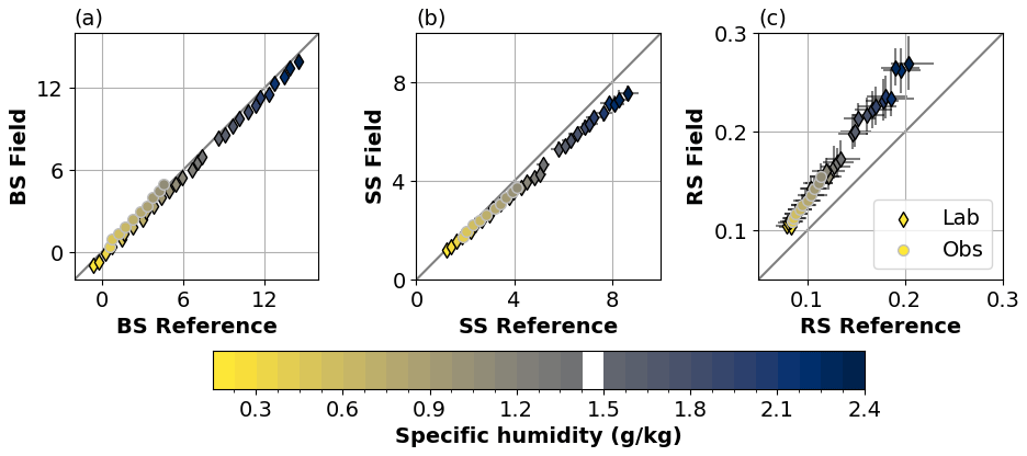
Figure 6 (a) Baseline shift, (b) slope shift, and (c) residuals of the expected model spectrum versus the fitted-absorption spectrum from the analyzer's WLM for field periods where the warm-box temperature is above the 95th or below the 5th percentiles. Light gray line represents 1-to-1 ratio. Data are divided into 0.075 g kg⁻¹ bins, from 0.15 to 2.4 g kg⁻¹ (color bar), with error bars denoting IQR for both field and reference measurements.

Table 3 Correlations and linear regression values (slope and intercept) for WLM metrics (baseline shift, BS; slope shift, SS; and residuals, RS) in field vs. reference period.

4.2 Measurement quality of water vapor isotopes

Based on the assessment of analyzer parameters presented above, measurement conditions within the ISE-CUBE system and in the laboratory differ mostly with respect to the variability of T_WB and T_DAS. To identify a potential impact of this temperature variability on the vapor isotope measurements, we now compare the variability of the isotopic signal between our reference periods and the field. Since mixing ratio (and thus the amount of molecules in the measurement cavity) is a key factor in the precision of the CRDS measurements, we divide the measurement data into 15 bins from 0.150 to 2.400 g kg⁻¹, 0.150 g kg⁻¹ wide, similar to the bins we used before in Sect. 4.1.3, though twice as wide.

For our field period, we first partition our measured humidities by site; in this way, we ensure that measurement conditions at each site are represented. Then, we identify the distribution of measured humidities at each site according to our bins and normalize it to 100 for the Snow site and 200 for the Fjord site. Then, occurrence in each bin is rounded up to the nearest whole number, such that the smallest bin contains at least two points. Finally, for each site and bin, we identify a corresponding number of 5 min windows with the most stable mixing ratios (i.e., lowest standard deviation of humidity), as categorized by the mean across the 5 min. The maximum standard deviation across all 5 min windows in the field was 0.030 g kg⁻¹, with the median being 0.002 g kg⁻¹. A similar procedure was done for the observatory reference period, though standard deviations were lower than in the field. Within the laboratory benchmark, we focus on 10 distinct usage events conducted for instrument characterization purposes (Fig. B1). During these events, the analyzer was subjected to stepwise mixing ratio sequences between 0.20 and 2.25 g kg⁻¹ (Fig. B1). The steps usually lasted 5 to 10 min, and the sequences did not necessarily follow a consistent step magnitude. Similar to the field and observatory setup, the most stable 5 min windows were identified using a cut-off threshold of 0.006 g kg⁻¹. These sequences used a standard of a similar depletion (δ¹⁸O: $-\mathrm{40.02}\pm \mathrm{0.07}$ ‰ and δD: $-\mathrm{307.8}\pm \mathrm{0.8}$ ‰) as our field measurements. For laboratory, observatory and field, the 1σ 5 min standard deviation over each of these windows was then calculated for both δ¹⁸O and δD.

For all three periods and for both δ¹⁸O and δD, the measurement precision decreases with decreasing mixing ratio (Fig. 7a, c). The same is true of the d-excess (Fig. 7e). In the lowermost bin of 0.150 to 0.300 g kg⁻¹, 5 min standard deviations in the field reach up to 1.0 ‰ for δ¹⁸O (Fig. 7a) and 8 ‰ for δD and the d-excess (Fig. 7c, e), whereas the same in the laboratory reference are around 0.7 ‰ (δ¹⁸O) and 5 ‰ (δD and d-excess). Across all humidities, field bin means (thick colored line) are consistently higher than laboratory and observatory bin means (Fig. 7a, c, e; black, gray and white lines, respectively). This difference between field and reference periods (Fig. 7b, d, f) increases at lower humidities, and is consistent between reference periods. A logarithmic fit (Fig. 7b, d, f; thick colored lines) gives the maximum increase in measurement uncertainty (at the minimum humidity value from the field, 0.197 g kg⁻¹) as 0.15 ‰ for δ¹⁸O, 1.35 ‰ for δD and 1.42 ‰ for d-excess. According to this fit, the median humidity value from the field (0.562 g kg⁻¹) would have associated increases of uncertainty in δ¹⁸O, δD and d-excess of 0.10 ‰, 0.89 ‰ and 0.93 ‰, respectively. Averaged across humidity bins, this corresponds to a variability increase of 30 % in the field compared to the laboratory benchmark, though the largest relative increase occurs at the higher humidities.

Figure 7 Standard deviations of δ¹⁸O, δD and d-excess in field and reference periods, alongside differences between periods. Measurements organized across 0.15 g kg⁻¹ bins, from 0.15 to 2.40 g kg⁻¹. (a) Standard deviations of δ¹⁸O over 5 min periods from field (colored “x”), laboratory (black “+”) and observatory (gray “o”); see text for details. Bin means depicted with thick lines. (b) Differences between bins means from field and laboratory (black ticks) and field and observatory (gray circles) periods. Thick colored line indicates the logarithmic fit of field–lab differences. (c, d) Same as panels (a) and (b) but for δD. (e, f) Same as panels (a) and (b) but for d-excess.

In summary, the field deployment exhibits consistently higher variability for isotopic measurements as compared to the optimal measurement conditions in a well-controlled research laboratory. This higher variability in the field is likely a consequence of the more variable T_WB and T_DAS but could also be due to the more variable composition of the ambient air used to quantify stability. Additionally, we have not investigated the contribution that our increased flow configuration (Sect. 2.2) might make to this increase in variability. Therefore, we proceed under the premise that our obtained measurements have an increased uncertainty associated with the conditions and the deployment system, as described by the calculated logarithmic fits. Nonetheless, we will show that, though this decreased precision is inherent to the observations, it does not hinder useful measurements, particularly since the measurement precision is quantified.

4.3 Profiling-module performance

Evaluation of the profiling-module is divided into sensor performance and sample transmission. Sensor performance details of the ultrasonic distance sensor and the temperature probe at the tip of the inlet are found in Appendix C. We now assess the profiling module's ability to transmit samples to the analyzer, including its capacity to resolve isotopic profiles.

The time it takes for the analyzer to react to a step change in humidity at the inlet head is predominantly governed by the length of the inlet tubing and the flow rate through it. With the heated tubing from the inlet tip to the sample port of the analyzer having a diameter of 4.5 mm and a flow rate of about 9 L min⁻¹ in the profiling-module tubing and 0.15 L min⁻¹ in the inlet assembly, the minimum response time would be approximately 6 s. We were unable to conduct any controlled single-step changes during the field deployment, as we lacked a suitable field device to produce a defined vapor isotope stream at sufficiently high flow rates. However, profiling with the articulating arm approximated multiple step changes, albeit without a controlled humidity source. We take the profiling period from the Fjord site on 9 March 2020, which included multiple abrupt humidity changes as we stepped through profiling levels, with some step changes reaching 0.3 g kg⁻¹ (Fig. 8a). Therefore, we followed the approach of Steen-Larsen et al. (2014) and Wahl et al. (2021) and applied a fast Fourier transform analysis to the normalized time derivative of the specific humidity observed during this profiling period (Fig. 8b). We then consider the median across 20 logarithmically spaced bins, between $\mathrm{5.55}\times {\mathrm{10}}^{-\mathrm{3}}$ and 2 Hz, of the resulting power spectra as a signal-to-noise ratio (SNR; Fig. 8b, blue line), with the spectral minimum defining our baseline at approximately 0.4 Hz or 2.5 s. We see that the signal reaches 63 % of its full response after approximately 20 s; however, by 30 s the signal is 80 % of its full response. These statistics are also similar, though less strong, for the low humidities encountered at the Snow site (Fig. S4). Therefore, we conclude that the system is capable of producing a dataset with 30 s resolution, which can be used for analysis purposes.

Figure 8 Inlet response determination for the profiling period on 9 March 2020, from 12:57 to 15:30 UTC. (a) The 4 Hz specific-humidity signal as measured by the analyzer. (b) The fast Fourier transform of the normalized time derivative of the specific humidity (gray), expressed as a signal-to-noise ratio. Black line is the median of the resulting power spectra across 20 logarithmically spaced bins between $\mathrm{5.55}\times {\mathrm{10}}^{-\mathrm{3}}$ and 2 Hz, while colored shading is the IQR of the bin. The minimum of the median (at approximately 0.4 Hz or 2.5 s) serves as noise baseline, whereas the maximum signifies the full response (dashed gray line). Dotted line indicates 63 % of the full response.

Next, we consider the minimum duration required at a particular height to resolve the isotopic profile. We again take our profiling period on 9 March 2020, now examining the isotopic measurements (Fig. 9a, c, e). We apply a fast Fourier transform on the 4 Hz isotopic signal to obtain a power spectrum across a range of frequencies and periodicities (Fig. 9b, d, f). The spectra median (across 20 logarithmically spaced bins between $\mathrm{8.33}\times {\mathrm{10}}^{-\mathrm{4}}$ and 2 Hz; Fig. 8b, d, f; thick black lines) indicates a baseline extending from 2 Hz until approximately 0.1 Hz (10 s). Frequencies higher (periodicities smaller) than this are considered to be indistinguishable from noise. The 25th and especially the 75th percentiles for these frequencies are also mostly constant (Fig. 9b, d, f; colored shading). At periods larger than 20 s, the signal begins to emerge from the noise. The d-excess signal takes the longest to emerge, with the median SNR surpassing the 75th percentile of the noise level (Fig. 9f; dotted line) at 1.5 min. This means that 50 % of the frequencies at this point have a higher SNR than 75 % of the noise. Periodicities smaller than this have less than 2 times as much power as the noise median and cannot be resolved. After 2 min, the median signal reaches 5 dB or approximately 3.16 times the median noise baseline; periodicities larger than this can begin to be resolved. At periodicities of 4 min, medians of all isotopic signals have an SNR larger than or equal to 10 dB. At the less humid Snow site, the median SNR is equal to or above 5 dB after 4 min (Fig. S5). Therefore, across both deployment sites, we determine that maintaining a single height for at least 4 min is necessary to begin to resolve the signal during profiling, though longer durations will yield a higher resolving power.

Figure 9 Resolving isotopic signals during the profiling period on 9 March 2020, from 12:57 to 15:30 UTC. (a) The 4 Hz δ¹⁸O signal (gray), with the 30 s mean (thick black) and standard deviation of the same (colored shading). (b) The fast Fourier transform of δ¹⁸O (gray), expressed as a signal-to-noise ratio. Black line is the median of the resulting power spectra across 20 logarithmically spaced bins between $\mathrm{8.33}\times {\mathrm{10}}^{-\mathrm{4}}$ and 2 Hz, while colored shading is the IQR of the bin. Dotted line is the mean of the 75th percentile for frequencies larger than 0.1 Hz. (c, d) Same as panels (a) and (b) but for δD. (e, f) Same as panels (a) and (b) but for d-excess.

4.4 Cold-trap module performance

The cold-trap expansion module was fully integrated into the sample airflow of the ISE-CUBE system during the field tests. Since the cold-trap box was not thermally regulated, the cryocooler unit was operated well below the manufacturers minimum operating guideline of 5 ^∘C, reaching −5 ^∘C over sustained periods and even down to −20 ^∘C occasionally. Nonetheless, the cryocooler reliably provided temperatures of $-\mathrm{80}\pm \mathrm{5}$ ^∘C at the base of the vial enclosure for 80 % of the deployment. The remaining 20 % mostly occurred during overnight collections, whereby excessive frost buildup on the exterior of the brass vial enclosure would provide additional insulation, and the vial temperature would drop below −85 ^∘C. Vapor collection in a vial lasted between 8 and 16 h during daytime and nighttime, with target flow rates of 0.5 and 0.25 L min⁻¹, respectively. Water vapor was successfully collected during a total of 28 periods, with up to 0.3 mL in a single sample, though some samples collected significantly less.

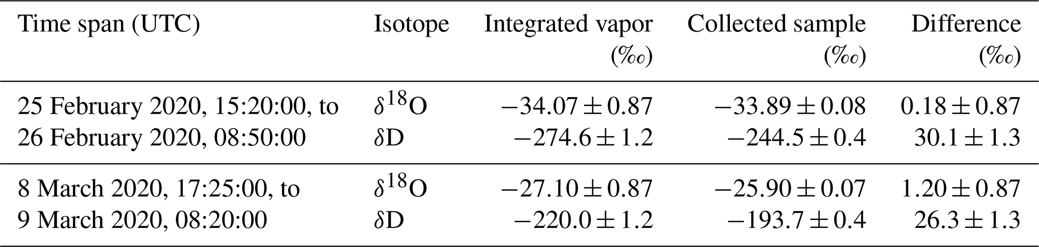
We now present a comparison between two collected samples and the mass-flow-integrated isotope measurements from the analyzer for the same period (Table 4). One sample is from during the Snow deployment, while the other is from the time at the Fjord. While δ¹⁸O values are close to being within measurement error, the δD values are quite different. This is likely due to a combination of deficiencies involving sample collection, inconsistent flow regulation and possibly fractionation effects at the low temperatures in the glass sample vial. These fractionation effects might arise from incomplete freeze-out of the vapor, induced by insufficient thermal stability of the glass collection vial. We additionally observed substantial ice crystal formation in the neck of the collection vials, which inhibited and decreased flow during multiple collection periods. This ice formation also compromised sample recovery during vial exchange, causing frozen samples to fall out of the vial during collection. Therefore, the disagreement between sample and analyzer measurements is not unexpected, especially as the collected samples would no longer correspond with the integrated time period being compared.

Table 4 δ¹⁸O and δD measurements for two time periods, as observed by the CRDS analyzer (integrated vapor) and as collected by the cold trap (collected sample), alongside the differences between.

In summary, we provide here a first proof of concept that a cryocooler-based cold-trap module can be integrated into the ISE-CUBE system. The deficiencies identified could be corrected with a different collection vial and a better flow regulator (i.e., a mass flow controller), although the sample analysis procedure would need to be changed. A more detailed evaluation of the performance of the cold-trap module in terms of sampling efficiency and its suitability for in-field calibration is, however, beyond the scope of this paper and will be detailed in a future publication.

4.5 Example of a profiling operation

We now present an example for a profiling operation at the Fjord site on the afternoon of 9 March 2020, from 12:57 to 15:30 (UTC). Winds during this period were fairly constant around 7 m s⁻¹, occasionally gusting to 9 m s⁻¹. The entire profiling operation consisted of a sequence of 19 steps across three cycles, performed at heights between 1.5 and 3.5 m above the surface of the water (Fig. 10a, black line). Throughout the profiling operation, mean air temperature at the inlet and mean specific humidity were anti-correlated with height (Fig. 10a, cyan and blue lines, respectively). The profiling head was kept at any particular height for 4.5 to 13 min (Fig. 10a, yellow highlights), with the first 30 s at the level disregarded. For these periods, we calculated the corresponding means for the humidity, temperature, δ¹⁸O, δD and d-excess (Fig. 10b–e, colored markers), alongside the standard errors of the means with a 99 % confidence interval (Fig. 10b–e, black error bars). We also calculated the observed variability (standard deviation) of the measured quantities (Fig. 10b–e, gray error bar), including the system uncertainty as calculated in Sect. 4.2 (Fig. 10c–e, gray ticks on error bar). We found the variability to be a similar magnitude for all height levels regardless of sampling duration, with the system uncertainty accounting for approximately half the variability at any particular height.

Across the 2 m profile span, a linear fit through the mean humidities yielded a gradient (with 95 % confidence interval) of $-\mathrm{0.13}\pm \mathrm{0.04}$ $\left(\mathrm{g}{\mathrm{kg}}^{-\mathrm{1}}\right){\mathrm{m}}^{-\mathrm{1}}$ (Fig. 10b, blue). The linear fit for air temperature was $-\mathrm{0.63}\pm \mathrm{0.17}$ K m⁻¹ (Fig. 10b, cyan). This was to be expected, as the surface of the water was a source of both heat and moisture. The isotopic signature of the moisture also exhibited a gradient; δ¹⁸O, δD and the d-excess (Fig. 10c, d, e) all display negative gradients across their linear fits ($-\mathrm{0.86}\pm \mathrm{0.49}$ ‰ m⁻¹, $-\mathrm{13.4}\pm \mathrm{5.3}$ ‰ m⁻¹ and $-\mathrm{6.52}\pm \mathrm{2.17}$ ‰ m⁻¹, respectively). The profiles, especially those for δD and the d-excess, have a strong correlation with height, and the derived linear gradients have a narrow 95 % confidence interval (Fig. 10b–e; black shading).

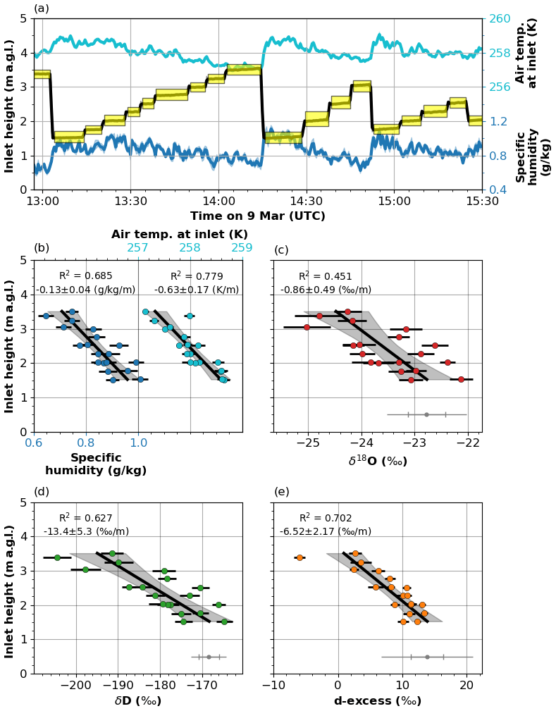
Figure 10 A profiling operation from 12:57 to 15:30 UTC on 9 March 2020. (a) A time series of inlet head height (black lines, left axis), alongside the air temperature at the same (cyan line, upper-right axis) and specific humidity (blue line, lower-right axis). A total of 19 height levels and their durations are denoted with yellow highlighting. (b) Vertical profiles of the air temperature at the inlet head (cyan, upper-right axis) and specific humidity (blue, bottom-left axis). Error bars signify standard errors, with 99 % confidence interval. Thick black line is the linear regression through the data points, with shading showing 95 % confidence interval. (c) Same as panel (b) but for δ¹⁸O. (d) Same as panel (b) but for δD. (e) Same as panel (b) but for d-excess. The lower gray marker and error bar is a variability scale denoting a representative standard deviation for any particular height, with system uncertainty, as calculated in Sect. 4.2, indicated as ticks.

5 Discussion

With the ability to resolve near-surface profiles, the ISE-CUBE system offers a number of advantages over a valve–manifold combination. Fundamentally, the profiling arm allows for increased continuity in the observed profiles as compared to a fixed height tower. The freedom to choose any height in the 2 m range enabled us to produce fine-scale vertical profiles with a resolution of approximately 25 cm. Though this particular interval is arbitrary, being able to select heights of interest while measuring led to a more dynamic sampling strategy that could be adapted on the fly. Duplicating a profile such as that obtained on 9 March would involve an 8-fold increase in the number of inlet lines without any guarantee that an inlet would be at a height of interest. Unlike typical tower measurements, the short inlet lines of the profiling module allow for rapid instrument response and limit potential wall interactions with the tubing during sample transmission. These short inlet lines are only possible due to the relatively small size of the ISE-CUBE stack (as compared to previous, larger enclosures) and the thin silhouette of the profiling frame, which limits flow distortion. In addition, the flexibility of the measurement height with the articulating arm is a clear asset for measurements over water surfaces with strong tidal variation. Finally, it would be quite possible to deploy alongside a tower with fixed height inlets, as these towers have the advantage of automated sampling over much longer time periods. A measurement strategy like this would provide information on the rapidly occurring surface processes alongside the more long-term, continuous context in which they are taking place.

Speculation on such a measurement strategy might imply that the ISE-CUBEs could be deployed for longer periods. However this prototype has a practical time limitation imposed by calibration necessity. Currently, the integrated cold trap is unsuitable to be used for calibrating CRDS measurements. However, if one could integrate a field calibration module into the system, the system could very likely stand on its own for extended periods of time. While the analyzer and pump modules could be used without the profiling module for an extended deployment, at some duration the benefits of a more conventional enclosure would begin to warrant additional effort during installation. A larger enclosure (such as a pre-existing building) offers a level of security that the ISE-CUBEs cannot provide for long-term measurement efforts that are less concerned with small-scale processes which do not necessarily require a long deployment to observe.

Regardless of deployment length, the current ISE-CUBE system is limited by the lack of an active temperature control capability, which presently prevents operation in warmer measurement environments. With the modular approach, the addition of a dedicated ventilation module with larger fans and active cooling–heating unit is straightforward and would enable deployment in warmer and more variable climatic conditions. Preliminary testing with such a module has already yielded promising results in ambient temperatures up to around 20 ^∘C, though shielded from direct sunlight (Sect. S2).

One potential internal change in our measurement setup would involve the high-flow mode described in Sect. 2.2. This mode enabled 4 Hz sampling and enhanced instrument response time. However, it is unexplored regarding whether the measurement precisions found in Sect. 4.2 might be improved if the instrument were to remain in standard low-flow mode. Were this the case, the inlet assembly would need to be modified to even further reduce the amount of tubing subjected to this decreased flow and to maintain fast instrument response.

6 Conclusions and outlook

In this work, we have detailed the design and performance of the new ISE-CUBE system for near-surface profiles of water vapor isotope measurements. The modular design enables rapid installation, while the compact system size provides minimized flow distortion around the measurement site and allows us to measure in stable conditions with shallow boundary layers.

During a 2-week-long field experiment in Ny-Ålesund, Svalbard, Norway, during February–March 2020, the analyzer encountered extreme environmental conditions while deployed in the ISE-CUBEs. Though ambient temperatures reached down to −30 ^∘C, the analyzer remained within its specified range of measurement conditions with regard to T_C, T_WB, T_DAS and p_C. Measurement precisions during the field deployment were, on average, 0.10 ‰ (δ¹⁸O) and 0.93 ‰ (δD) lower than in the reference benchmarks.

The profiling module, a height-adjustable sampling arm with a range of 2 m, enabled profiling of the water isotope composition throughout the shallow surface layer in a stable atmosphere. With a response time of approximately 20 s, the ISE-CUBE system captured profiles and gradients in this layer. Even at the low humidities (down to 0.25 g kg⁻¹) over the tundra, the profiles achieve a high-enough signal-to-noise ratio to resolve the vertical isotopic gradients after approximately 4 min at each height interval. Due to the high vertical resolution in the profiles, the observed gradients are robust.

Integration of the cold-trapping expansion module based on the design of Peters and Yakir (2010) into the ISE-CUBE system enabled quantitative vapor collection. Samples were typically collected over a duration of 8 h or more in low-humidity environments, resulting in a maximum collection of 0.3 mL at a time. Such cold trapping enables subsequent liquid-sample analysis in a laboratory environment for quality control of the calibration and the measurement of H${}_{\mathrm{2}}^{\mathrm{17}}$O for triple-isotope capability. While the cold-trap module is functional, the preliminary results provided here show that design refinements are necessary.

The modular nature of the system invites additional expansion. A top-priority expansion module would focus on an in-field calibration system. In general, there are multiple potential calibration devices using a variety of vapor generation methods (Iannone et al., 2009; Gkinis et al., 2010; Ellehoj et al., 2013); the device just needs to be robust and suitably compact, all while generating a consistent source of known vapor. For example, Leroy-Dos Santos et al. (2021) have put forward an instrument that can generate stable vapor streams down to 0.045 g kg⁻¹ (70 ppmv), one of which has been operating mostly autonomously in Antarctica, with little manual intervention. Further potential expansion modules include a battery power module, which would permit mobile operation. In addition to an enhanced ventilation module, an enhanced, autonomous profiling module would remove the need for nearby operators, removing any chance of human-induced error in the stable water isotope measurements.

Deployments need not be limited to measurements of stable water isotopes. Many laser spectrometers for other atmospheric trace gases, such as methane, carbon dioxide or carbon isotopes, may be integrated into the system and used for purposes beyond meteorology and/or hydrology; those produced by, but not limited to, Picarro would most readily fit the system. With a more robust temperature controller, there is the possibility for deployment in more temperate environments. Such locations may include, but are not limited to, glaciers, sea ice, lakes, coastal areas, caves, forests, grasslands, croplands, deserts and other places where evaporation and condensation interactions with the surface contribute to the vapor isotope composition of the near-surface atmosphere.

The availability of a modular, versatile deployment system such as the ISE-CUBE implies easy access to remote locations and environments while maintaining necessary data quality standards. As we provide the design in a easily reproducible way to the community (see the Supplement), we endeavor to enable further development and widespread acquisition of high-quality datasets from previously inaccessible measurement locations.

Appendix A: ISE-CUBE component list

Table A1 Components used in the ISE-CUBE system. General gas connections (PTFE tubing, unions, reducers, etc.) are made with parts from Swagelok Inc. Files for 3D-printed ventilation mounts were custom-made and are not listed (see the Supplement). Modular abbreviations are as follows: AN = analyzer module; PU = pump module; CT = cold-trap module; PR = profiling module.

Appendix B: Laboratory benchmark sequences

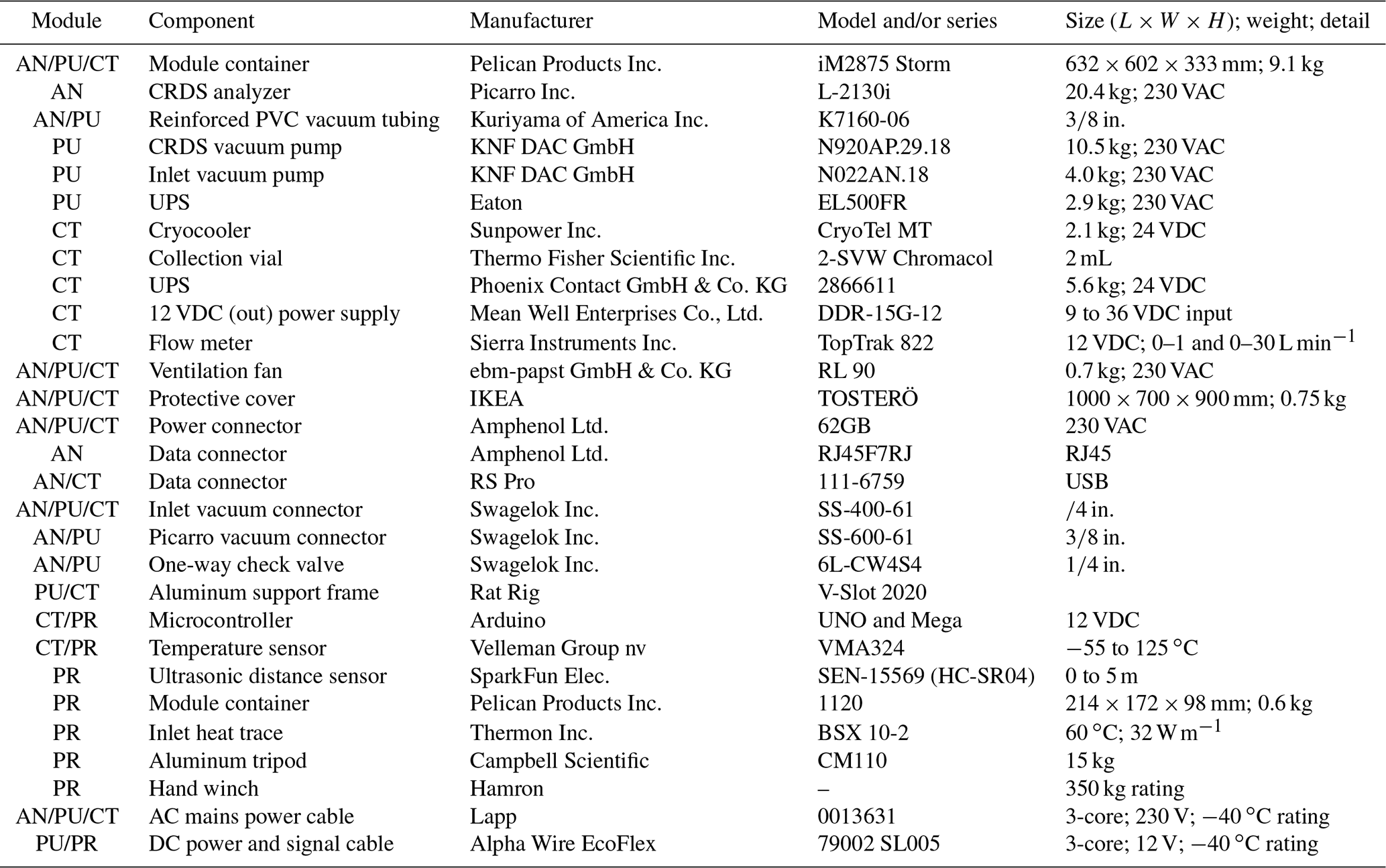
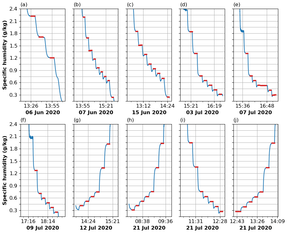
Figure B1 Humidity step sequences from 10 (a–j) distinct usage events from laboratory characterization of the analyzer during the period of June to July 2020. Blue line depicts volumetric mixing ratio, with red highlights showing 5 min periods with a standard deviation less than 0.006 g kg⁻¹. Panels (a)–(c) used 100 % nitrogen as the carrier gas, while panels (d)–(j) used synthetic air (80 % N₂, 20 % O₂). All events used a lab standard of a similar depletion (δ¹⁸O: $-\mathrm{40.02}\pm \mathrm{0.07}$ ‰ and δD: $-\mathrm{307.8}\pm \mathrm{0.8}$ ‰) as measured in the field.

Appendix C: Profiling-module sensor performance

The distance given by the ultrasonic sensor was periodically checked against a manual tape measure throughout the field deployment (accuracy $\pm \sim \mathrm{2}$ cm). The behavior of the ultrasonic sensor did vary between the two measurements sites, likely as a result of underlying surface. While deployed over snow, the sensor functioned with 2 cm accuracy over the range of 50 to 205 cm. When the inlet head was lowered below 50 cm, the sensor gave unreliable and clearly spurious measurements. We speculate that the particular type of ultrasonic sensor used was affected by the acoustic properties of the snowpack below this threshold. In these circumstances, manual distance was taken with a tape measure, with corresponding markings made on the controlling steel cable. No issues with distance sensors were encountered while deployed at the Fjord location with water or sea ice at the surface. At both locations, we observed a low signal-to-noise ratio and a jumpy distance signal during strong winds (>11 m s⁻¹), possibly due to the ultrasonic pulse being advected away before the reflected signal was received.

The temperature sensor above the tip of the inlet of the profiling module was compared against the temperature sensor of an automated weather station (Jocher et al., 2012; Schulz, 2017) (20 m away) at a height of 100 cm for 37 h (during 25 and 26 February). The 1 min averaged temperature records of the two sensors show a high correlation of 0.991, with a linear regression slope of 1.000±0.005 (Fig. C1). The profiling sensor consistently recorded higher temperatures than the automated weather station, having a linear regression offset of 0.6 ^∘C. While the distance between sensors might account for some of this discrepancy, the gradients observed with the profiling module are almost 1 order of magnitude larger, with relative changes well captured due to the high linearity. Overall, the sensors installed on the profiling module functioned adequately.

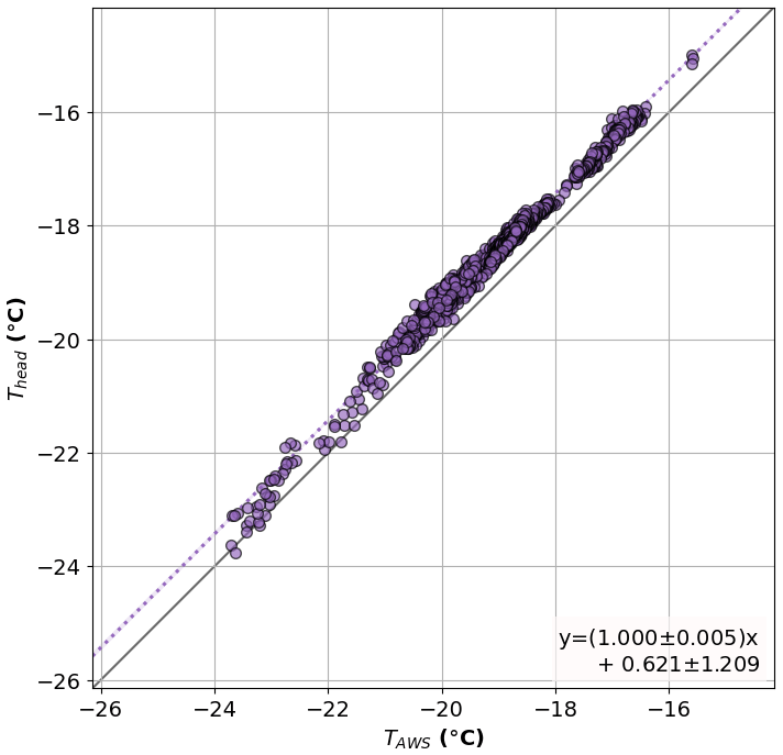
Figure C1 Comparison between the temperature sensor of the automated weather station (T_AWS) and the inlet temperature sensor (T_head). Both were at a height of 100 cm above the surface of the snow for 37 h. Solid gray line represents 1-to-1 ratio. Dotted line indicates linear regressions through the data points, with purple shading (barely visible under dotted line) showing the 95 % confidence interval.