the Creative Commons Attribution 4.0 License.
the Creative Commons Attribution 4.0 License.
 | 16 Feb 2023
High-resolution 3D winds derived from a modified WISSDOM synthesis scheme using multiple Doppler lidars and observations
Chia-Lun Tsai
Kwonil Kim
Yu-Chieng Liou
GyuWon Lee
The WISSDOM (Wind Synthesis System using Doppler Measurements) synthesis scheme was developed to derive high-resolution 3-dimensional (3D) winds under clear-air conditions. From this variational-based scheme, detailed wind information was obtained from scanning Doppler lidars, automatic weather stations (AWSs), sounding observations, and local reanalysis datasets (LDAPS, Local Data Assimilation and Prediction System), which were utilized as constraints to minimize the cost function. The objective of this study is to evaluate the performance and accuracy of derived 3D winds from this modified scheme. A strong wind event was selected to demonstrate its performance over complex terrain in Pyeongchang, South Korea. The size of the test domain is 12×12 km2 extended up to 3 km a.m.s.l. (above mean sea level) height with a remarkably high horizontal and vertical resolution of 50 m. The derived winds reveal that reasonable patterns were explored from a control run, as they have significant similarity with the sounding observations. The results of intercomparisons show that the correlation coefficients between derived horizontal winds and sounding observations are 0.97 and 0.87 for u- and v-component winds, respectively, and the averaged bias (root mean square deviation, RMSD) of horizontal winds is between −0.78 and 0.09 (1.77 and 1.65) m s−1. The correlation coefficients between WISSDOM-derived winds and lidar QVP (quasi-vertical profile) are 0.84 and 0.35 for u- and v-component winds, respectively, and the averaged bias (RMSD) of horizontal winds is between 2.83 and 2.26 (3.69 and 2.92) m s−1. The statistical errors also reveal a satisfying performance of the retrieved 3D winds; the median values of wind directions are −5 to 5 (0 to 2.5)∘, the wind speed is approximately −1 to 3 m s−1 (−1 to 0.5 m s−1), and the vertical velocity is −0.2 to 0.6 m s−1 compared with the lidar QVP (sounding observations). A series of sensitivity tests with different weighting coefficients, radius of influence (RI) in interpolation, and various combination of different datasets were also performed. The results indicate that the present setting of the control run is the optimal reference to WISSDOM synthesis in this event and will help verify the impacts against various scenarios and observational references in this area.
- Article
(10471 KB) - Full-text XML
- BibTeX
- EndNote


In the past few decades, many practical methods have been developed to derive wind information by using meteorological radar data (Mohr and Miller, 1983; Lee et al., 1994; Liou and Chang, 2009; Bell et al., 2012). The derived winds substantially revealed reasonable patterns compared with conventional observations (such as surface stations, soundings, wind profiles, etc.) and models (Liou et al., 2014; North et al., 2017; Chen, 2019; Oue et al., 2019). Most comprehensive applications of the derived winds were adopted to document kinematic and precipitation structures associated with various weather systems or phenomena at different scales from thousands (cold fronts and low-pressure systems, LPSs), to hundreds (tropical cyclones and typhoons), and to a couple of kilometers (convective lines and tropical cyclone rainbands; it naturally depends on the length and width of the rainbands) (Yu and Bond, 2002; Yu and Jou, 2005; Yu and Tsai, 2013, 2017; Tsai et al., 2018; Yu et al., 2020; Cha and Bell, 2021; Tsai et al., 2022). In addition, the accuracy of 3-dimensional (3D) winds could be improved when increasing the number of Doppler radars because relatively fewer assumptions and more information can be included (Yu and Tsai, 2010; Liou and Chang, 2009). Therefore, the retrieved schemes within multiple Doppler radars are a more popular way to obtain high-quality 3D winds and have been extensively applied to meteorological analyses.
The technique of velocity track display (VTD; Lee et al., 1994) and ground-based velocity track display (GBVTD; Lee et al., 1999) can derive the winds from a single Doppler radar under some assumptions, as the wind patterns are generally uniform or axisymmetric rotational (Cha and Bell, 2021). More extended techniques based on VTD and GBVTD have also been applied to increase the quality of derived wind data, and such techniques include extended GBVTD (EGBVTD; Liou et al., 2006) and generalized velocity track display (GVTD; Jou et al., 2008). However, winds usually present nonuniform patterns and fast-evolving characteristics in most mesoscale weather systems and microscale phenomena, and complete and detailed winds are still difficult to resolve by these techniques. Most developed techniques are based on the contexts of weaknesses from the above schemes on wind retrievals. Instead of a single Doppler radar, multiple Doppler radars can retrieve better-quality 3D winds with relativity fewer assumptions because they provide sufficient radial velocity measurements and wind information with wider coverage in the synthesis domain.
Cartesian Space Editing, Synthesis, and Display of Radar Fields under Interactive Control (CEDRIC; Mohr and Miller, 1983) is a traditional package used to retrieve 3D winds by dual-Doppler radar observations. This scheme usually determines the horizontal winds by using two radars, and the vertical velocity can be obtained by variational adjustment with the anelastic continuity equation. Spline Analysis at Mesoscale Utilizing Radar and Aircraft Instrumentation (SAMURAI) software is another way to retrieve 3D winds (Bell et al., 2012); this scheme is a kind of variational data assimilation that adopts multiple radars. Recently, Tsai et al. (2018) utilized the measurements of six Doppler radars to document precipitation and airflow structures over complex terrain on the northeastern coast of South Korea via Wind Synthesis System using Doppler Measurements (WISSDOM; Liou and Chang, 2009). The scientific studies and applications of WISSDOM were well documented in Liou et al. (2012, 2016). In addition, the immersed boundary method (IBM; Tseng and Ferziger, 2003) was applied in WISSDOM. Since one of the advantages of WISSDOM is that it considers the orographic forcing on Cartesian coordinates by applying the IBM, higher-quality 3D winds can be derived well over terrain (Liou et al., 2013, 2014; Lee et al., 2018).
Generally, radial velocity is measured by detecting the movement of precipitation particles relative to the locations of Doppler radars; thus, there are no sufficient radial velocity measurements under clear-air conditions. However, the winds in clear-air conditions usually play an important role in the initiation of various weather systems and phenomena, such as downslope winds, gap winds, and wildfires (Reed, 1931; Colle and Mass, 2000; Mass and Ovens, 2019; Lee et al., 2020). Although surface stations, soundings, and wind profilers can measure winds under clear-air conditions, relatively poor spatial coverage is still a problem for obtaining sufficient wind information in certain local areas. Therefore, scanning Doppler lidars will be one approach to obtain wind information under clear-air conditions. Päschke et al. (2015) assessed the quality of wind derived by Doppler lidar with a wind profiler in a year-long trial, and the results showed good agreement in wind speed (the error ranged between 0.5 and 0.7 m s−1) and wind direction (the error ranged between 5 and 10∘). Bell et al. (2020) combined an intersecting range height indicator (RHI) of six Doppler lidars to build “virtual towers” (such as wind profilers) to investigate the airflow over complex terrain during the Perdigão experiment. These virtual towers can fill the gap in wind measurements above meteorological towers. The uncertainty of wind fields is also reduced by adopting multiple Doppler lidars (Choukulkar et al., 2017), and a high spatiotemporal resolution of derived wind allows small-scale rotors in mountainous areas to be checked (Hill et al., 2010).
The original WISSDOM was designed to retrieve 3D winds based on Doppler radar observations and background inputs combined with conventional observations and modeling. However, the original WISSDOM only provided 3D winds under precipitation conditions. It does not work well under clear-air conditions because Doppler radar cannot easily detect radial velocity without precipitation particles. To obtain high-quality 3D winds under clear-air conditions, the radial velocity observed from the scanning Doppler lidars can be used in the modified WISSDOM. The results will allow us to investigate the initiation of precipitation systems in advance of rainfall and snowfall, which is an essential benefit over Doppler radar data. Furthermore, the conventional observations and modeling datasets were used as isolated constraints in the modified WISSDOM synthesis scheme. One of the benefits of the isolated constraints is that it is easy to synthesize any kind of wind information obtained from available datasets and give suitable weighting coefficients with different constraints when they are processing the minimization in the cost function. Thus, more reliable 3D winds in clear-air conditions were derived well from this modified WISSDOM synthesis scheme.
The objective of this study is to modify the WISSDOM synthesis scheme based on the original version to be a more flexible and useful scheme by adding any number of Doppler lidars and conventional observations, as well as modeling datasets. This modified WISSDOM will allow us to obtain an exceedingly high spatial resolution of 3D winds (50 m was set in this study) under clear-air conditions. A resolution of 50 m was chosen in this study, as the Doppler lidars' respective horizontal resolution averages 40–60 m. A variety of adequate datasets were collected during a strong wind event in the winter season during an intensive field experiment ICE-POP 2018 (International Collaborative Experiments for PyeongChang 2018 Olympic and Paralympic winter games). In summary, the main goal of this study is to use Doppler lidar observations to retrieve high-resolution 3D winds over terrain with clear-air conditions via WISSDOM. In this study, detailed principles of the modified WISSDOM and data implementation are elucidated in the following sections. In addition, the modified WISSDOM was used to retrieve 3D winds over complex terrain under clear-air conditions in a strong wind event. The reliability of the derived 3D winds was also evaluated and discussed with respect to conventional observations.
2.1 Original version of WISSDOM (Wind Synthesis System using Doppler Measurements)
WISSDOM is a mathematically variational-based scheme to minimize the cost function, and various wind-related observations can be used as one of the constraints in the cost function. The 3D winds were derived by variationally adjusted solutions to satisfy the constraints in the cost function; thus, this is a gradient descent technique to converge toward a solution. The original version of WISSDOM utilized five constraints, including radar observations (i.e., reflectivity and radial velocity), background (combined with automatic weather station, sounding, model, or reanalysis data), continuity equation, vorticity equation, and Laplacian smoothing (Liou and Chang, 2009). Liou et al. (2012) applied the IBM in WISSDOM to consider the topographic effect on the non-flat surfaces. One of the advantages of IBM is providing realistic topographic forcing without changing the Cartesian coordinate system into a terrain-following coordinate system. More scientific documentation associated with the interactions between terrain, precipitation, and winds in different areas can be found in Liou et al. (2016) for Taiwan and in Tsai et al. (2018) for South Korea. The cost function can be expressed as
where JM is the different constraints. J1 is the constraint related to the geometric relation between radar radial Doppler velocity observations (Vr) and the derived one from true winds () in Cartesian coordinates (Eq. 2). Note that Vt is first estimated based on the background of the sounding observations used in this study. In the absence of background observations, the first guess of Vt is set to 0.
Since WISSDOM is a scheme that uses the 4DVAR (4D variational method) approach, the variations between different time steps (t) should be considered, and two time steps of radar observations were collected in this constraint and all following constraints. The x, y, z indicates the location of a given grid point in the synthesis domain, and i could be any number (N) of radars (at least 1). The α1 is the weighting coefficient of J1 (α2 is the weighting coefficient of J2 and so on). in Eq. (2) is defined as Eq. (3):
(Vr)i,t is the radial velocity observed by the radar (i) at time step (t), and , , and depict the coordinate of radar i. The ut, vt, and wt (WT,t) denote the 3D winds (terminal velocity of precipitation particles) at given grid points at the time step t; and .
The second constraint is the difference between the background (VB,t) and true (derived) wind field (), which is defined as
There were several options to obtain background in the original version of WISSDOM. The most popular background resource involves using sounding observations; however, it can only provide homogeneous wind information for each level in WISSDOM with relatively coarse temporal resolution (3 to 12 h intervals). The other option is combining sounding observations with AWS (automatic weather station) observations. Although the AWSs provided wind information with better temporal resolution (1 min), the data were only observed at the surface layer with semi-random distributions. The last option is to combine sounding, AWS, modeling, or reanalysis datasets. However, various datasets with different spatiotemporal resolutions are not favorable for the appropriate interpolation of given grid points of WISSDOM synthesis, and the accuracy and reliability of the background may have been significantly affected by such a variety of datasets. Thus, these different observed or modeled data should be treated differently to minimize uncertainties and improve accuracy. Therefore, one of the improvements in the modified WISSDOM is that these inputs were individually separated into independent constraints with flexible interpolation methods. In addition, individual constraints were calculated in two time steps if the temporal resolution of the inputs was high enough. The sounding observations are still a necessary dataset because the air density and temperature profile were used to identify the height of the melting level. In this study, sounding winds were adopted to represent the background for each level and a constraint at the same time; nevertheless, the AWS and reanalysis datasets are independent constraints in the modified WISSDOM (details are provided in the following section).
The third, fourth, and fifth constraints in the cost function are the anelastic continuity equation, vertical vorticity equation, and Laplacian smoothing filter, respectively. Equations (5), (6), and (7) are denoted as follows:
ρ0 in Eq. (5) is the air density, and in Eq. (6). The main advantage is that using vertical vorticity can provide further improvement in winds and thermodynamic retrievals from a method named the terrain-permitting thermodynamic retrieval scheme (TPTRS; Liou et al., 2019).
2.2 The modified WISSDOM
In addition to the five constraints in the original version, the modified WISSDOM synthesis scheme includes three more constraints in the cost function. Thus, the cost function in the modified WISSDOM was written as
J1 to J5 in Eq. (8) are the same constraints corresponding to Eqs. (2)–(7). The main purpose of this study is to retrieve 3D winds under clear-air conditions in which observational data are relatively rare. Instead of the radial velocity observed from Doppler radars in Eq. (3) in the original version of WISSDOM, the radial velocity observed from Doppler lidars was adopted in the modified WISSDOM synthesis. In addition, if there were no precipitation particles under clear-air conditions, the terminal velocity of precipitation particles (WT,t) was set to zero in Eq. (3) in the modified WISSDOM. In this study the time steps in WISSDOM are set to 12 min, corresponding to the temporal resolution of the primary input lidar data. Relatively minor changes in environmental conditions were assumed in WISSDOM due to the limitation on the coarse temporal resolution from specific inputs. For example, the closest time step of a sounding observation or LDAPS (Local Data Assimilation and Prediction System) dataset was chosen regarding the synthesis time, and the time constraint was set to be the same.
The sixth constraint is the difference between the derived wind fields and the sounding observations (VS,t), as defined in Eq. (9):
The sounding data in J6 were interpolated to the given grid points near its tracks bearing on the radius influence (RI) distance (the details are provided in Sect. 3.2.3). The main difference between J6 and J2 is that the sounding data with various wind speeds and directions were used as an observation for given 3D locations in J6 instead of the constraint of homogeneous background winds (i.e., uniform wind speed and direction) for each level in the studied domain in J2. An additional benefit of J6 is that any number of sounding observations can be efficiently adopted in the WISSDOM synthesis domain. The seventh constraint represents the discrepancy between the true (derived) wind fields and AWS data (VA,t), as expressed in Eq. (10):
Finally, the eighth constraint measures the misfit between the derived winds and the local reanalysis dataset (VL,t), as defined in Eq. (11):
In this study, various observations and reanalysis datasets were utilized as constraints in the cost function of WISSDOM. The most important dataset is the radial velocity observed from Doppler lidars, which can measure wind information with high spatial resolution and good coverage from near the surface up to higher layers in the test domain. Sounding and AWSs can provide horizontal winds for background or that should be included in the constraints. The local reanalysis datasets were obtained from the 3DVAR (3D variational) Local Data Assimilation and Prediction System (LDAPS) data assimilation system from the Korea Meteorological Administration (KMA). Since these datasets have different coordinate systems and various spatiotemporal resolutions, additional procedures are required before the synthesis. Detailed descriptions of the procedures are described in the next section.
The high-quality synthesized 3D wind field from radar observations has been applied in several previous studies such as those by Liou and Chang (2009), Liou et al. (2012, 2013, 2014, 2016), and Lee et al. (2017). The advantages and details of WISSDOM can be found in Tsai et al. (2018). Although several studies have used Doppler radar in WISSDOM, this study is the first to apply Doppler lidar data in WISSDOM. This modified WISSDOM synthesis scheme has also been applied in the analysis related to the mechanisms of orographically induced strong wind on the northeastern coast of Korea (Tsai et al., 2022). In contrast to previous studies, this study provides clear context, detailed procedures, reliability, and the limitations of the modified WISSDOM.
3.1 Basic information of WISSDOM synthesis
A small domain near the northeastern coast of South Korea was selected to derive detailed 3D winds over complex terrain (in the black box in the inset map in Fig. 1) because relatively dense and high-quality wind observations were only collected in this region during ICE-POP 2018. The size of the WISSDOM synthesis domain is 12×12 km2 (up to 3 km a.m.s.l.; above mean sea level) in the horizontal (vertical) direction with 50 m grid spacing. Such high-spatial-resolution 3D winds were synthesized every 1 h in this test. The output time steps are adjustable to be finer (recommended limitation is 10 mins), but they are highly related to the temporal resolution of various datasets and computing resources. Two scanning Doppler lidars are located near the center of the domain: one is the equipped “WINDEX-2000” (the model's name from the manufacturer) at the May Hills Supersite (MHS), and the other is the “Stream line-XR” at the Daegwallyeong regional weather office (DGW) site. In addition to the operational AWSs (727 stations), additional surface observations (32 stations) are also involved in ICE-POP 2018 surrounding the MHS and DGW sites and the venues of the winter Olympic Games. The soundings were launched at the DGW site every 3 h during the research period. The LDAPS also provided high spatial resolution of wind information in the test domain. The horizontal distribution of all instruments and datasets used are shown in Fig. 1.
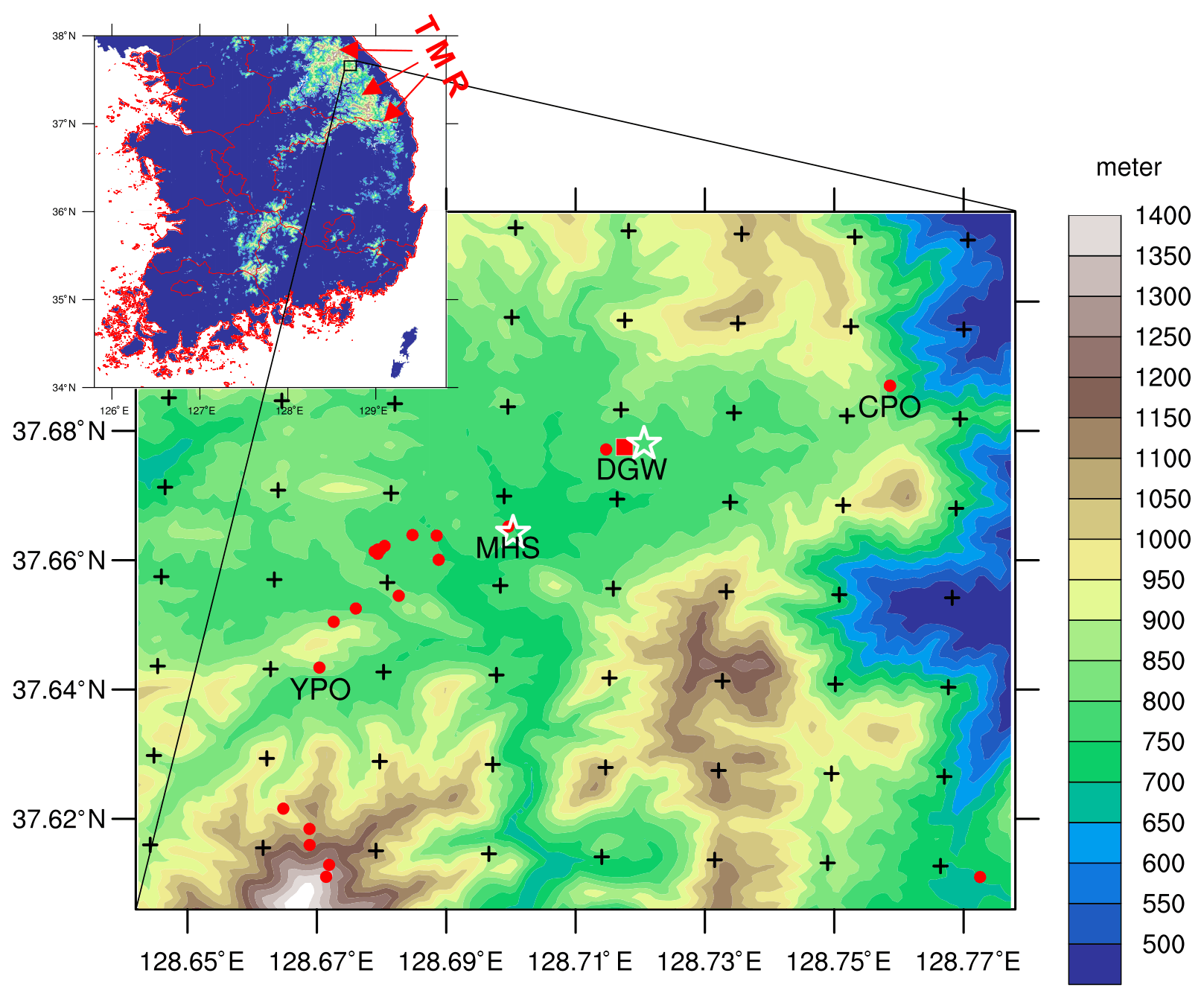
Figure 1Horizontal distribution of instruments and datasets used in this study. A small box in the upper map indicates the WISSDOM synthesis domain. The Doppler lidars are marked by start symbols at the MHS and DGW sites. Solid red circles and the square indicate the automatic weather stations (AWSs) and sounding, respectively. The black cross marks the data points of LDAPS. Topographic features and elevations are shown with the color shading in a color bar in the figure. The location of the Taebaek mountain range (TMR) is also marked.
3.2 Data implemented in WISSDOM synthesis
3.2.1 Scanning Doppler lidars
The radial velocity observed from two scanning Doppler lidars was utilized to retrieve 3D winds via WISSDOM synthesis. The original coordinate system of observed lidar data is not a Cartesian coordinate system but a spherical (or polar) coordinate system as a plan position indicator (PPI) and hemispheric range height indicator (HRHI) or the RHI. Although relatively dense and complete coverage of wind information (i.e., radial velocity of aerosols) was sufficiently recorded by lidar observations, the collected data are usually not located directly on the given grid points in the WISSDOM synthesis (i.e., Cartesian coordinate system). In this study, the lidar data were interpreted simply from the lidar coordinate system to the Cartesian coordinate system via bilinear interpolation.
The scanning strategy of the lidar at the DGW site includes five elevation angles for PPI (7, 15, 30, 45, and 80∘ before 10:00 UTC on 14 February 2018 and 4, 8, 14, 25, and 80∘ after 10:00 UTC) and two HRHIs at azimuth angles of 51 and 330∘. A full volume scan included all PPIs and HRHIs every ∼12 min. The maximum observed radius distance is ∼13 km, and the grid spacing is 40 m for each gate along the lidar beam. The scanning strategy of the lidar at the MHS site involves seven elevation angles for PPI (5, 7, 10, 15, 30, 45, and 80∘) and one HRHI at an azimuth angle of 0∘. A full volume scan included all PPIs and RHIs every ∼12 min. The maximum observed radius distance was ∼8 km, and the grid spacing was 60 m. The vertical distribution of lidar data in the test domain is shown as blue lines in Fig. 2a.
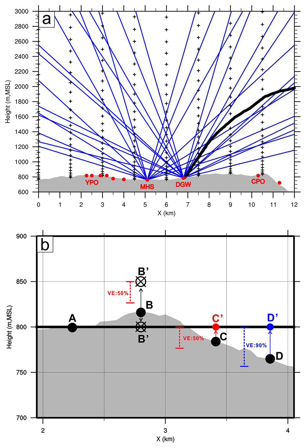
Figure 2(a) Schematic diagram of the vertical distribution of adopted lidar datasets. Blue lines indicate the lidar data observed at the DGW and MHS sites with different elevation angles. The AWSs are located on the ground and are marked by solid red circles. An example of a sounding track launched from the DGW site in one time step (06:00 UTC on 14 February 2018) is plotted as a thick black line. The black cross marks indicate the vertical distribution of the LDAPS dataset. (b) Schematic diagram for data implementation with various locations of the AWSs and different percentages of VE (vertical extension) from given grid points at 800 m a.m.s.l. (thick black line). The gray shading on the bottom represents the topography.
3.2.2 Automatic weather station (AWS)
Most of the AWSs are not exactly located on the given grid points of the Cartesian coordinate system. Objective analysis (Cressman, 1959) is a popular way to correct semi-random and inhomogeneous meteorological fields into regular grid points. This study adopted objective analysis for the AWS observations with adjustable RI distances between 100 and 2000 m. After this first step, the observational data can reasonably interpolate to the given grid points horizontally. Furthermore, an additional step is required to put these interpolated data into the given grid points at different vertical levels because the AWSs are located at different elevations in the test domain. In the traditional way of the original WISSDOM, the interpolated data are moved to the closest level with the shortest distance just above the AWS site. However, the interpolated data are not moved to the closest level if the shortest distances are large, like by more than half (50 %) of the grid spacing. Nevertheless, to include more data from the AWS observations appropriately, adjusted distances between the AWS sites and given grid points at different vertical levels were necessarily considered. These adjusted distances can be named vertical extension (VE) here, and there are two options of 50 % and 90 % in the tests of this study, which correspond to 25 and 45 m extensions between each grid (in the case the grid spacing is 50 m), respectively. An example demonstrated how to implement the interpolated data to the given grid points by adjustable VE after step one (Fig. 2b).
In Fig. 2b, the interpolated data do not need to move to a given grid point (as an example, at the 800 m level here) if the elevation of the AWS is equal to the height of a given grid point, like point A. When the AWS is located higher than a given grid point (like point B in Fig. 2b) and does not reach the lower boundary of VE (50 %) from the upper given grid point (i.e., at the 850 m level), these interpolated data will be removed and wasted. In contrast, when the interpolated data are located just below the given grid point with 50 % VE, it will be achieved in the WISSDOM synthesis at the 800 m level (point C in Fig. 2b). The interpolated data of point D have a similar situation to point B; however, it will be achieved at the 800 m level because a higher VE (90 %) was applied here. Since the locations of the AWSs are semi-random with relatively sparse or concentrated distributions, the optimal RI and adjustable VE make it possible to include more AWS observations in the WISSDOM synthesis.
3.2.3 Sounding
During ICE-POP 2018, the soundings are launched at the DGW site every 3 h (from 00:00 UTC). Vertical profiles of air pressure, temperature, humidity, and wind speed and direction were recorded every second (i.e., ∼3 m vertical spatial resolution) associated with the rising sensor. The sounding sensor drifted when rising, and an example of its track in one time step is shown as a thick black line in Fig. 2a. In this example, the sounding movement was mostly affected by westerly winds, and it measured the meteorological parameters in any location along the track in the test domain. The coordinate system of sounding data is quite similar to the distribution of AWS measurements, and the observations are not located right on the given grid points of the WISSDOM synthesis.
Similar to the AWS data, the sounding data also underwent objective analysis with an adjustable RI distance for the wind measurements in the first step. Then, the interpolated data were switched to given grid points for each vertical level by the different VEs in the WISSDOM synthesis.
3.2.4 Reanalysis dataset: LDAPS
The local reanalysis dataset LDAPS was generated by the KMA. This dataset provides u- and v-component winds every 3 h, and the horizontal spatial resolution is ∼1.5 km with the grid type in Lambert conformal (as black cross marks in Fig. 1). The data revealed denser distributions near the surface and sparse distributions at higher levels (see Fig. 2a). The initiation of wind variables in the LDAPS was assimilated with many observational platforms, including radar, AWS, satellite, and sounding data. Thus, the relatively high reliability of this dataset could be expected. In addition, such datasets have also significantly improved the forecast ability for small-scale weather phenomena over complex terrain in Korea (Kim et al., 2019; Choi et al., 2020; Kim et al., 2020).
The LDAPS data are not located directly on the given grid points of the WISSDOM synthesis system. Unlike the distribution of AWS and sounding observations, LDAPS has dense and good coverage in the test domain. The Cartesian coordinate system is the most efficient method and the best system for partial differential equations (Armijo, 1969), and it is also used in the cost function of WISSDOM (Liou and Chang, 2009). In this study, the horizontal and vertical resolutions of given grid points were primarily determined by the characteristics of lidar data. Therefore, similar to lidar observations, the LDAPS data were also interpolated to the given grid points on the Cartesian coordinate system via the bilinear interpolation method.
3.3 Overview of the selected strong wind event
A strong wind event was selected to evaluate the performance of this modified WISSDOM synthesis scheme. In this strong wind event, the evolution of surface wind patterns on the Korean Peninsula was mainly dominated by a moving LPS, which is one type of strong downslope wind (Park et al., 2022; Tsai et al., 2022). The LPS moved out from China and penetrated the northern part of the Korean Peninsula through the Yellow Sea beginning at approximately 12:00 UTC on 13 February 2018. Consequently, a relatively strong surface wind speed (exceeding ∼17 m s−1) was observed when the LPS was located near the northeastern coast of the Korean Peninsula (40∘ N, ∼130∘ E) at 00:00 UTC on 14 February 2018 (Fig. 3). Then, the surface wind speed became weak when the LPS moved away from South Korea after 00:00 UTC on 15 February 2018 (not shown); the details of the synoptic conditions can be found in Tsai et al. (2022).
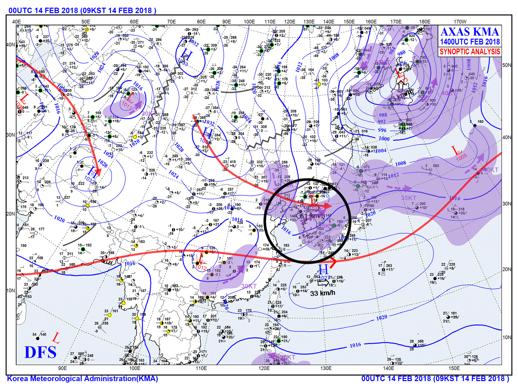
Figure 3Synoptic surface chart from the Korea Meteorological Administration (KMA) at 00:00 UTC on 14 February 2018. The location of the Korean Peninsula and the LPS has been marked by black circle.
This event is one of two strong wind events (i.e., daily maximum wind speeds larger than 10 m s−1 observed at the AWS sites along the northeastern coast of South Korea) in the past decade based on the KMA historic record. Such a strong wind event may help us to examine the potential maximum errors in the retrieved winds. Since persistent, strong westerly winds were observed by the soundings and AWSs from near the surface and upper layers over the Taebaek mountain range (TMR) during the event, the data coverage in the test domain was checked during a chosen time step (06:00 UTC on 14 February 2018). The percentage of data occupations for each dataset (after interpolation) was checked, and the results are shown in Fig. 4. Note that the elevation of the TMR is approximately 700 m a.m.s.l. in the test domain. The lidars provided good coverage of 100 % to 50 % at the lower layers between 700 m and 800 m a.m.s.l. The coverage of lidars was reduced significantly above 900 m a.m.s.l. and remained at ∼5 % due to the scan strategy during the Olympic Games (more dense observations near the surface). The maximum coverage of the AWS observations is ∼40 % at 800 m, and there was less coverage above this layer since relatively few AWSs are located in the higher mountains. Because only one sounding observation was utilized in this domain, relatively little coverage was also depicted. The local reanalysis LDAPS can provide complete coverage above 900 m a.m.s.l. (exceeding 100 %), albeit there was less coverage in the lower layers due to terrain. The lidar, sounding, and AWS observations covered most areas at lower levels but not higher levels; thus, the LDAPS compensated for most of the wind information at the upper layers in the WISSDOM synthesis.
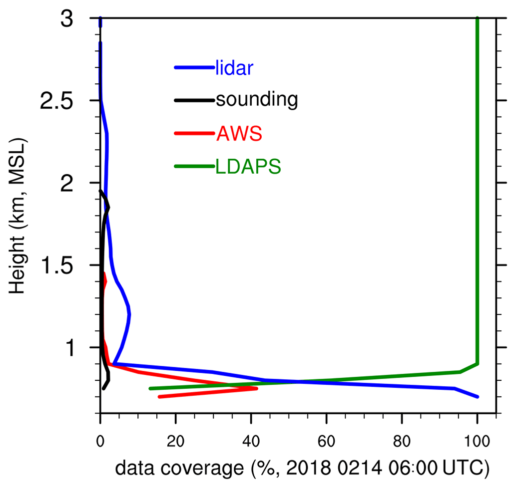
Figure 4Data coverage (percentage, %) of the lidar (blue line), sounding (black line), and AWS (red line) observations, as well as LDAPS (green line), at 06:00 UTC on 14 February 2018.
4.1 Control run
Relatively reliable 3D winds were derived by a control run of the WISSDOM synthesis because all available wind observations and local reanalysis datasets were appropriately acquired. These datasets provided sufficient and complete wind information with a high percentage of coverage in the test domain (see Fig. 4). Therefore, the retrieved winds from the control run can be treated as the optimal results in WISSDOM. The control run was performed carefully with the necessary procedures in data implementation before running the WISSDOM synthesis as follows. The lidar and LDAPS datasets must perform bilinear interpolation to the given grid points in WISSDOM, and the sounding and AWS observations must undergo objective analysis with the appropriate RI distance and VE. The quantities of the weighting coefficients for each input dataset followed the default setting from the original version of WISSDOM. The 3D winds were derived during one time step at 06:00 UTC on 14 February 2018 and compared with conventional observations. The best weighting coefficients have been determined by a series of observation system simulation experiment (OSSE)-type tests from Liou and Chang (2009). They put more weight on observations and less on modeling inputs. Based on the experiences and the default setting of weighting coefficients from their studies, the basic setting of the control run was first decided. Consequently, sensitivity tests were performed to better understand the possible variations associated with different weighting coefficients when the lidar data were implemented. The basic setting of this control run is summarized in Table 1.
Table 1Basic setting of WISSDOM (control run).
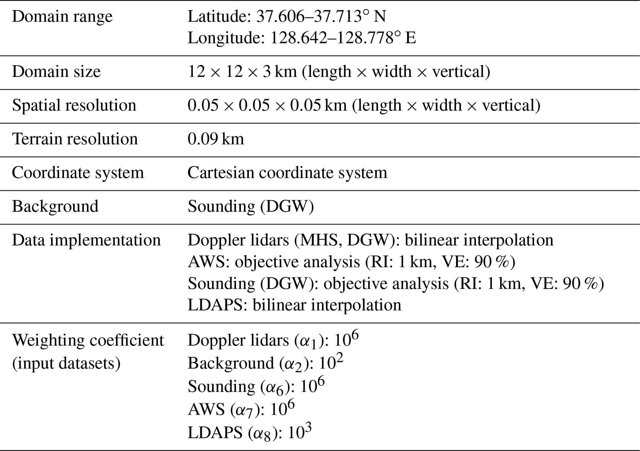
RI: radius influence; VE: vertical extension.
The results of 3D winds at 800 m a.m.s.l. derived from the control run are shown in Fig. 5a, c, and e. Topographic features comprised relatively lower elevations in the center of the test domain, and there were weaker u-component winds (∼7 m s−1) near the AWS and MHS lidar sites between 128.67 and 128.71∘ E (Fig. 5a). In contrast, the u-component winds (∼15 m s−1) were almost doubled near the DGW lidar site (between 128.71 and 128.73∘ E). The vertical structures of the u-component winds across these two lidars (i.e., along the black line in Fig. 5a) are shown in Fig. 5b. The strength of the u-component winds rapidly increased from the surface to the upper layers (from ∼6 to 20 m s−1), and uniform u-component winds with a wavy pattern were depicted above ∼1 km a.m.s.l. except for the stronger winds near the surface surrounding the DGW site. There were relatively weak (strong) u-component winds surrounding the lidar at the MHS (DGW) site near the surface. Relatively weak v-component winds were found (approximately ±4 m s−1) at 800 m a.m.s.l. (Fig. 5c); thus, the horizontal wind directions were mostly westerly winds during this time step. The v-component winds were obviously accelerated in several local areas encompassing the terrain (near 128.71∘ E). The vertical structure of the v-component winds (Fig. 5d) indicates that the v-component winds became stronger in the upper layer. The wind directions were changed from westerly to southwesterly from the near surface up to ∼1.4 km a.m.s.l. height. Updrafts were triggered on windward slopes when westerly winds impinged on the terrain or hills (Fig. 5e and f). Basically, the 3D winds derived from the WISSDOM synthesis reveal reasonable patterns compared to synoptic environmental conditions (see Fig. 3); the moving LPS accompanied stronger westerly winds.
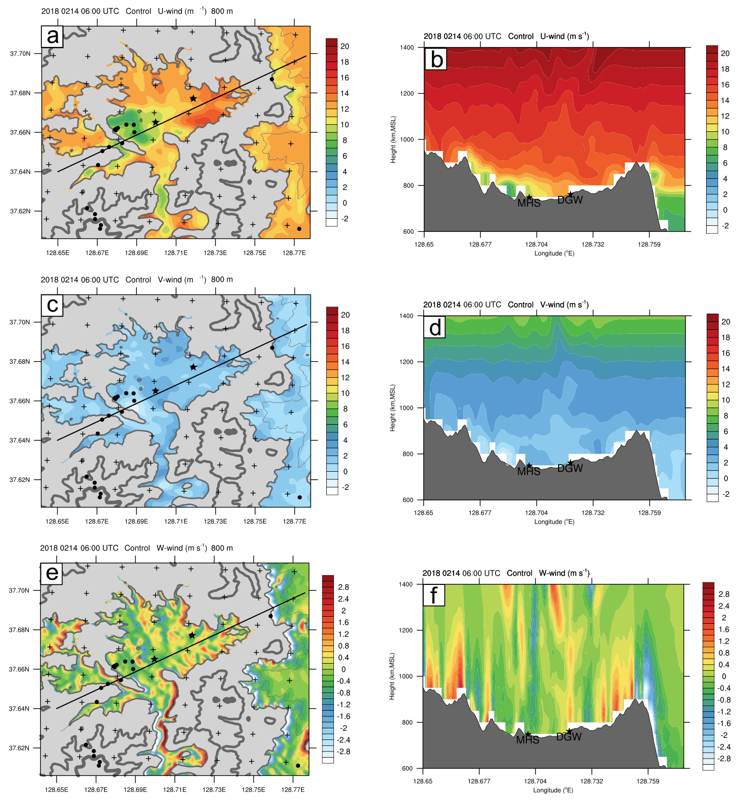
Figure 5The 3D winds were derived from the control run by the WISSDOM synthesis at 06:00 UTC on 14 February 2018. (a) The u-component winds (color, m s−1) at 800 m a.m.s.l.; the gray shading represents the terrain area, and the contours indicate different terrain heights of 600 m, 800 m, and 1000 m a.m.s.l. corresponding to thin to thick contours. The locations of lidars are marked with asterisks. (b) Vertical structures of u-component winds (color, m s−1) along the black line in panel (a). The gray shading in the lower part of the figure indicates the height of the terrain. Panels (c) and (d) are the same as panels (a) and (b) but for the v-component winds. Panels (e) and (f) are the same as panels (a) and (b) but for the w-component winds.
4.2 Intercomparison between derived winds and observations
Detailed analyses were performed in this section to quantitatively evaluate the accuracy of the optimally derived 3D winds from the WISSDOM synthesis. Two kinds of instruments were available in the test domain to detect the relatively realistic winds: sounding and lidar quasi-vertical profiles (QVPs; Ryzhkov et al., 2016). The QVPs of horizontal and vertical winds were retrieved based on the velocity–azimuth display (VAD) technique (Browning and Wexler, 1968; Gao et al., 2004). We regressed the Fourier coefficients of the Doppler velocities of the 80∘ PPI under the linear horizontal wind assumption and obtained the horizontal wind profile. The vertical (i.e., w-component) wind was retrieved under the assumptions of constant vertical wind, zero terminal velocity of aerosol particles, and no horizontal divergence (see Kim et al., 2022, for details on the wind retrieval). The accuracy of the retrieved wind profile is suitable for the WISSDOM wind evaluation, given the low root mean square deviation (RMSD) of <2.5 m s−1 and high correlation coefficient of >0.94 of horizontal wind speed as shown in the comparison against 487 rawinsondes (Kim et al., 2022). The horizontal winds observed from the soundings and the u-, v-, and w-component winds of the lidar QVP at the DGW site were utilized to represent the observations.
A complete analysis of the intercomparison between the WISSDOM synthesis and observations is presented in the following subsections. Because the verification observations are being used in the WISSDOM synthesis, the results of the control run are not verified independently; nevertheless, detailed discussions regarding the results of the sensitivity tests for the observations are presented in Sect. 5.
4.2.1 Sounding
The discrepancies between horizontal winds derived from WISSDOM and the sounding observations for the entire research period (from 12:00 UTC on 13 February to 12:00 UTC on 14 February 2018) were analyzed. Figure 6 shows the scatter plots of the u- and v-component winds on the locations following the tracks of soundings launched from the DGW site. Most of the u-component winds derived from WISSDOM are in good agreement with the sounding observations, and the wind speed is increased with the height from approximately 10 to 40 m s−1. A slight underestimation of retrieved u-component winds can be found at the layers of 1.5 to 2 km a.m.s.l. (Fig. 6a). In contrast, most of the v-component winds were weak (smaller than 15 m s−1) at all layers because the environmental winds were more like westerlies during the research period. There were also slightly overestimated v-component winds derived from WISSDOM at the layers of 1.5 to 2 km a.m.s.l. (Fig. 6b). The possible reason why the overestimated winds occurred above ∼1.5 km a.m.s.l. is that lidar data had relatively less coverage at higher layers (see Fig. 4).
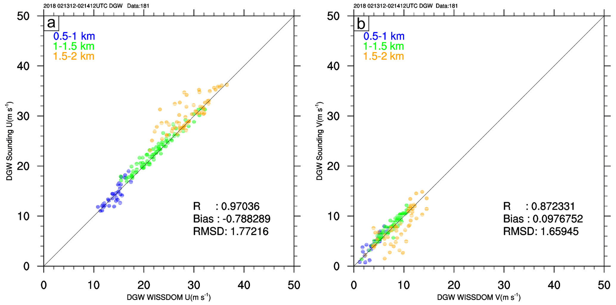
Figure 6Scatter plots of (a) u-component winds between the WISSDOM synthesis (x axis) and sounding observations (y axis) above the DGW site during the research period. The colors indicate different layers, and the numbers of data points, correlation coefficients, average biases, and root mean square deviations are also shown in the figure. (b) The same as panel (a) but for v-component winds.
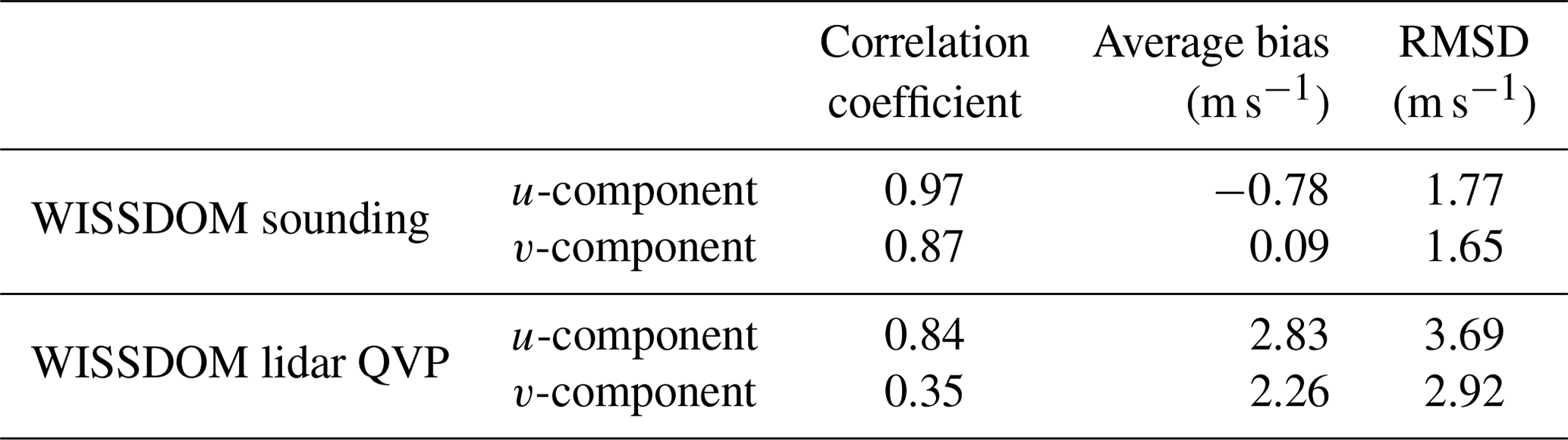
Overall, the u-component winds show a high correlation coefficient (exceeding 0.97), low average bias (−0.78 m s−1), and RMSD of 1.77 m s−1. The correlation coefficient of the v-component is also high (0.87), the average bias is 0.09 m s−1, and the RMSD is 1.65 m s−1.
The vertical profiles of the averaged u- and v-component winds for the period of 12:00 UTC on 13 February to 12:00 UTC on 14 February 2018 are shown in Fig. 7 for the WISSDOM synthesis (red) and sounding observations (black) launched from the DGW site. The average profiles agree well except for the height above 1.5 km a.m.s.l. and slight discrepancies in u- and v-component winds (<1 m s−1). Their statistical errors during the entire research period were quantified by the box plot shown in Fig. 8.

Figure 7Vertical wind profiles of average horizontal winds derived from the WISSDOM synthesis (red lines and vectors) and sounding observations (black lines and vectors) above the DGW site from 12:00 UTC on 13 February to 12:00 UTC on 14 February 2018. Solid lines indicate u-component winds (m s−1), and dashed lines indicate v-component winds (m s−1).
The maximum difference in wind directions between the WISSDOM synthesis and sounding observations is small at all layers. Relatively larger interquartile range (IQR) and median values can only be found at the lowest level. The IQR and median values of the wind direction differences are smaller (between ∼0 and 2.5∘) during the entire research period (Fig. 8a). Basically, the IQR and median values of the wind direction differences are close to 0∘ above 1 km a.m.s.l. Figure 8b shows the difference in wind speed between the WISSDOM synthesis and sounding observations. The differences in wind speed derived from WISSDOM were slightly underestimated in the layers between ∼0.85 and 1.3 km a.m.s.l. The median values of the wind speed differences were between −1 and 0.5 m s−1, and the IQRs of wind speed differences were between −2 and 0.5 m s−1. Above 1.3 km a.m.s.l., the differences in wind speed were small as their median values are close to 0 m s−1.
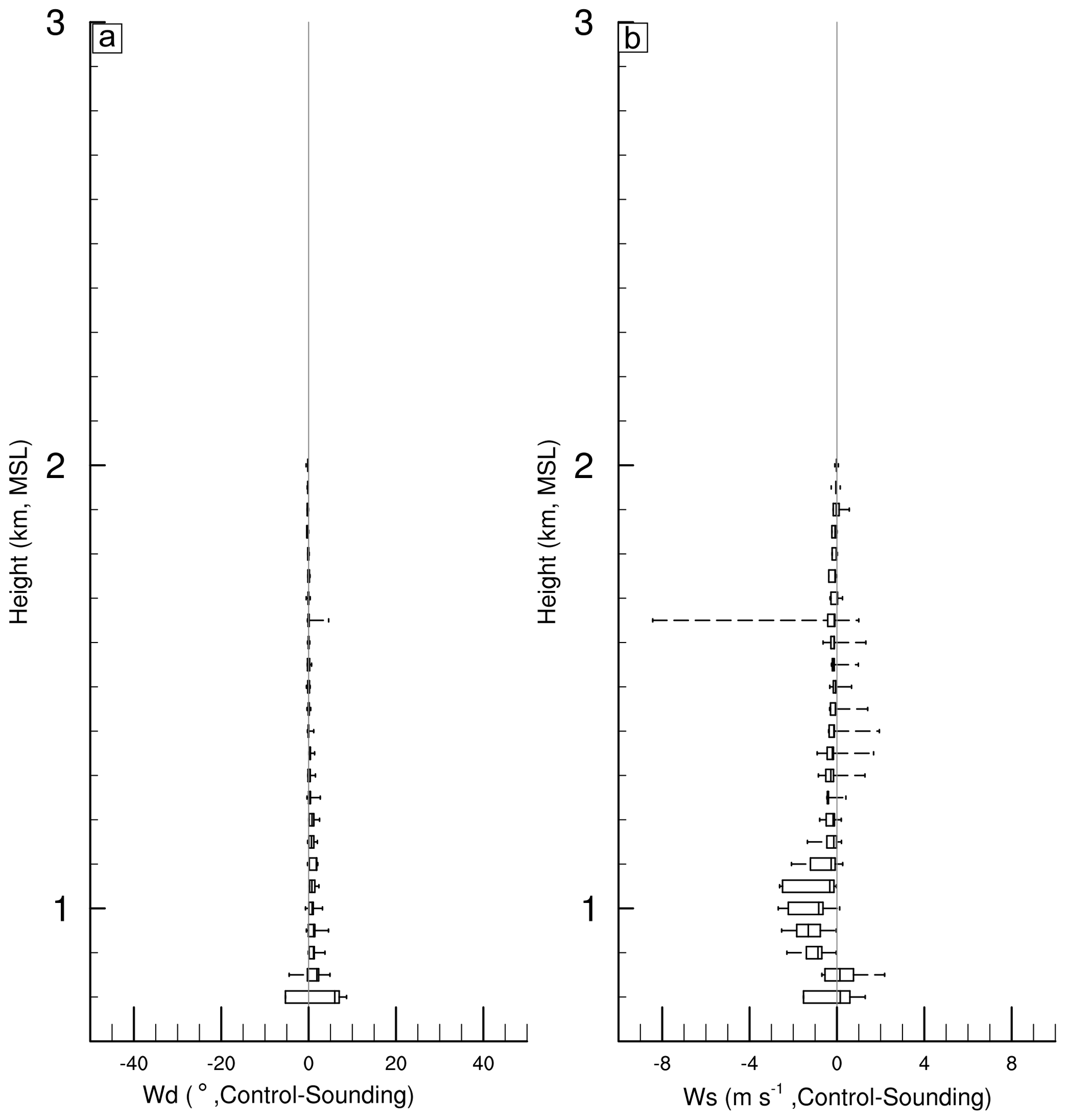
Figure 8The box plot of average (a) wind direction discrepancies between the WISSDOM synthesis and sounding observations above the DGW site during the research period. (b) Same as panel (a) but for the wind speed.
4.2.2 Lidar QVP
The lidar QVP is another observational reference used to evaluate the performance of derived winds from the WISSDOM synthesis. The scatter plots of the horizontal winds derived from WISSDOM and lidar QVP at the DGW site are shown in Fig. 9. The strength of the u-component winds increases with height in the range between approximately 10 and 40 m s−1 from the surface up to ∼2.5 km a.m.s.l. (Fig. 9a). Although the results show a relatively high correlation coefficient (0.84) for the u-component winds from lower to higher layers in the entire research period, the degree of scatter is larger than that in Fig. 6a. The average bias and RMSD of the u-component winds are 2.83 and 3.69 m s−1, respectively. The correlation coefficient of v-component winds is lower (0.35), associated with low wind speed (<15 m s−1) from the surface to 2.5 km a.m.s.l. (Fig. 9b), and it may possibly relate to less coverage from lidar QVP data at higher layers. The average bias and RMSD of the v-component winds are 2.26 and 2.92 m s−1, respectively. The results of these scatter plot analyses are summarized in Table 2. Basically, the u-component winds have high correlations, relatively lower bias, and lower RMSD than the v-component winds because the environmental winds are more westerly.
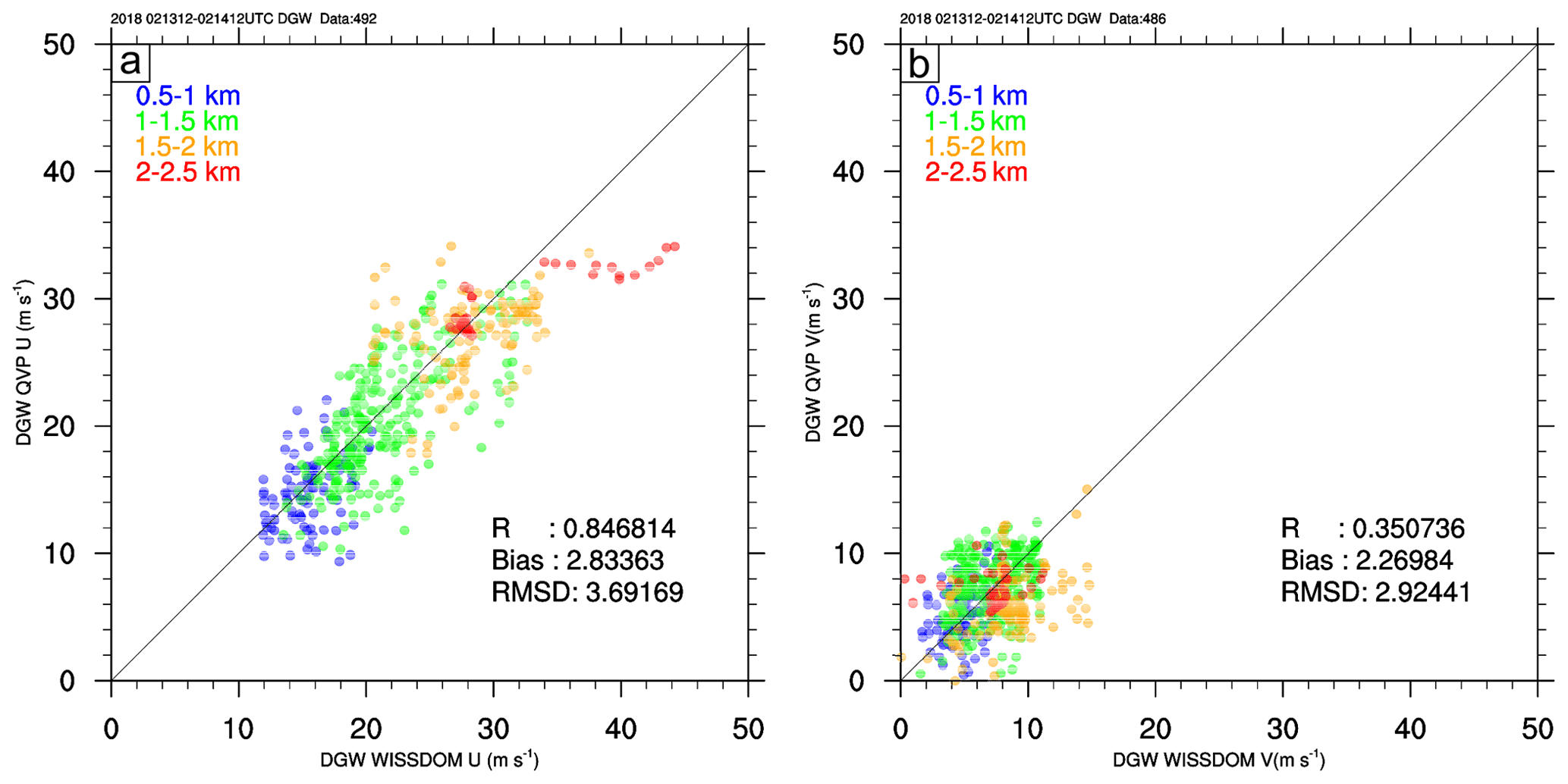
Figure 9The same as Fig. 6 but for (a) u-component winds between the WISSDOM synthesis (x axis) and lidar QVP (y axis). (b) The same as panel (a) but for v-component winds.
Table 2Summary of the intercomparisons between WISSDOM and observations.
Compared to the sounding observations, additional w-component winds are available in lidar QVP, which allows us to check their discrepancies in 3D winds. However, most of the vertical velocity observations were quite weak (approximately ±0.2 m s−1) above the DGW site, and the relatively low reliability of the derived vertical velocity could be expected in this event. Therefore, the average vertical profiles of 3D winds were utilized to qualitatively check the discrepancies between WISSDOM synthesis and lidar QVP during the research period (Fig. 10). The results show that the average u-component winds have relatively smaller discrepancies (approximately <1 m s−1) between the WISSDOM synthesis (marked as WISS-U in Fig. 10) and lidar QVP (marked as QVP-U) below ∼1.3 km a.m.s.l. at the DGW site. In contrast, there were larger discrepancies (approximately >2 m s−1) between 1.3 and 2 km a.m.s.l. The average v-component winds derived from WISSDOM (marked as WISS-V) and lidar QVP (QVP-V) were generally weak, and the ranges of WISS-V and QVP-V were between ∼2 and 8 m s−1. Generally, the vertical profiles of WISS-V were nearly overlain with QVP-V, and their discrepancies existed in the height range 1.6 to 2.0 km a.m.s.l. (maximum ∼4 m s−1). Smaller (larger) discrepancies in w-component winds were significantly below (above) the height at ∼1.3 km a.m.s.l. (maximum discrepancies ∼0.6 m s−1 at 1.7 km a.m.s.l.). Despite the larger discrepancies, the similar patterns of w-component winds can also be shown. In summary, the discrepancies in the 3D winds between the WISSDOM synthesis and lidar QVP were small in the lower layers and large in the higher layers because the observational data from lidars and AWSs provided good-quality and sufficient wind information at the lower layers but not in the higher layers (lower coverage of lidar data above 1.3 km a.m.s.l.; see Fig. 4).
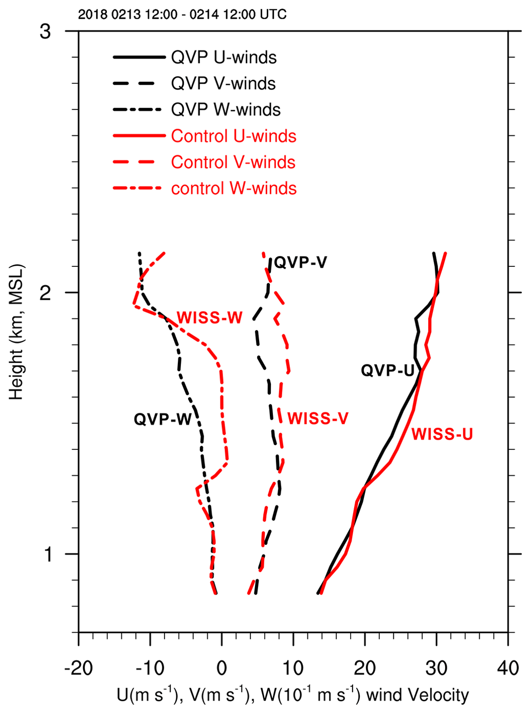
Figure 10Vertical wind profiles of average 3D winds derived from the WISSDOM synthesis (red lines and vectors) and lidar QVP (black lines and vectors) above the DGW site from 12:00 UTC on 13 February to 12:00 UTC on 14 February 2018. Solid lines indicate u-component winds (m s−1), dashed lines indicate v-component winds (m s−1), and dash-dotted lines indicate w-component winds (1×101 m s−1). The u-, v-, and w-component winds derived from the WISSDOM synthesis (lidar QVP) are marked by WISS-U (QVP-U), WISS-V (QVP-V), and WISS-W (QVP-W), respectively.
Figure 11 shows the quantile distribution of statistical errors in wind direction, wind speed, and vertical velocity between the WISSDOM synthesis and lidar QVP during the research period. The IQR of the wind direction is smaller (−5 to 5∘) in the layers from 0.85 to 1.5 km a.m.s.l. and turns to approximately −10 to 0∘ above 1.5 km a.m.s.l. The median values of wind direction are smaller (−5 to 5∘) from near the surface to the upper layers (Fig. 11a). Figure 11b shows that the median values (IQR) of wind speed are approximately −1 to 1 m s−1 (−2 to 2 m s−1) below 1.5 km a.m.s.l., and they all become larger with heights above 1.5 km a.m.s.l. (between −1 and 3 m s−1 for median values and −4 to 4 m s−1 for the IQR). The statistical error in the vertical velocity reveals that the IQR is −0.2 to 0.2 m s−1 (−0.8 to 0.8 m s−1) below (above) 1.3 km a.m.s.l., and the median values are 0–0.2 to −0.2 to 0.6 m s−1) below (above) 1.3 km a.m.s.l. The results of statistical errors are summarized in Table 3.
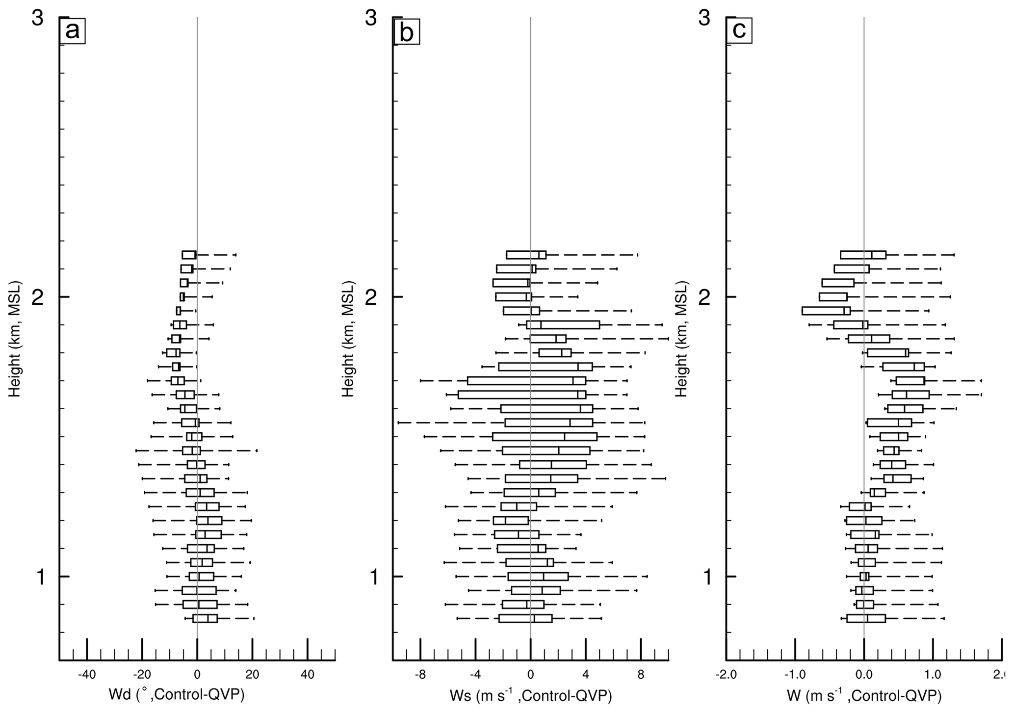
Figure 11The box plot of average (a) wind direction discrepancies between the WISSDOM synthesis and sounding observations above the DGW site during the research period. (b) Same as panel (a) but for the wind speed. (c) Same as panel (a) but for the w-component winds.
Table 3Summary of the statistical errors between WISSDOM and observations.
5.1 Impacts of various datasets (Experiment A)
In this section, the impacts of various datasets on data implemented in the WISSDOM synthesis were evaluated. In particular, the quantitative variances between each design, control run, sounding observations, and the QVP can be estimated. The basic setting of Experiment A took off several inputs from the WISSDOM control run (see Table 1) as four designs in Experiment A. The details of these four designs are summarized in Table 4 as the control run without the lidar observations (A-1), the control run without the AWS observations (A-2), the control run without the sounding observations (A-3), and the control run without the LDAPS data (A-4). The discrepancies in 3D winds were examined between the control run and each design in Experiment A. Since the environmental wind speed is nearly entirely comprised of uniform westerlies in this event, the results only show the difference in u-component winds between the control run and each design (A-1 to A-4) in Fig. 12. An additional test was designed, in which only Doppler lidar data are used without other constraints from J6 to J8 (A-5) to evaluate the performances between the modified and original versions of WISSDOM.
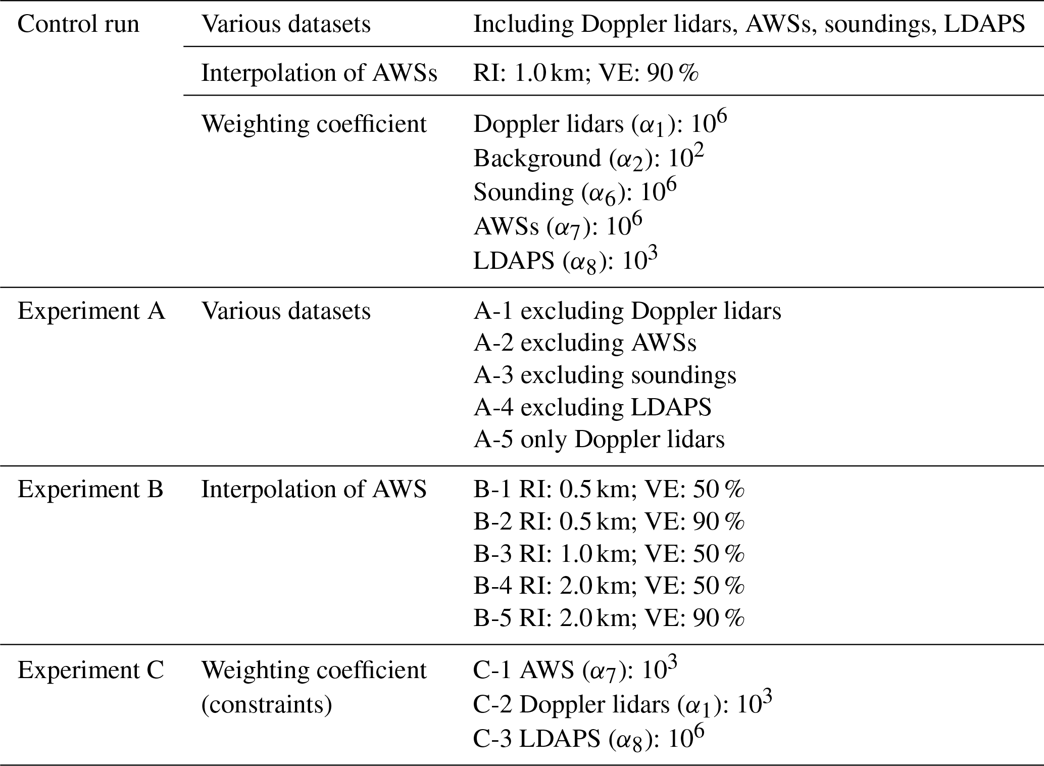
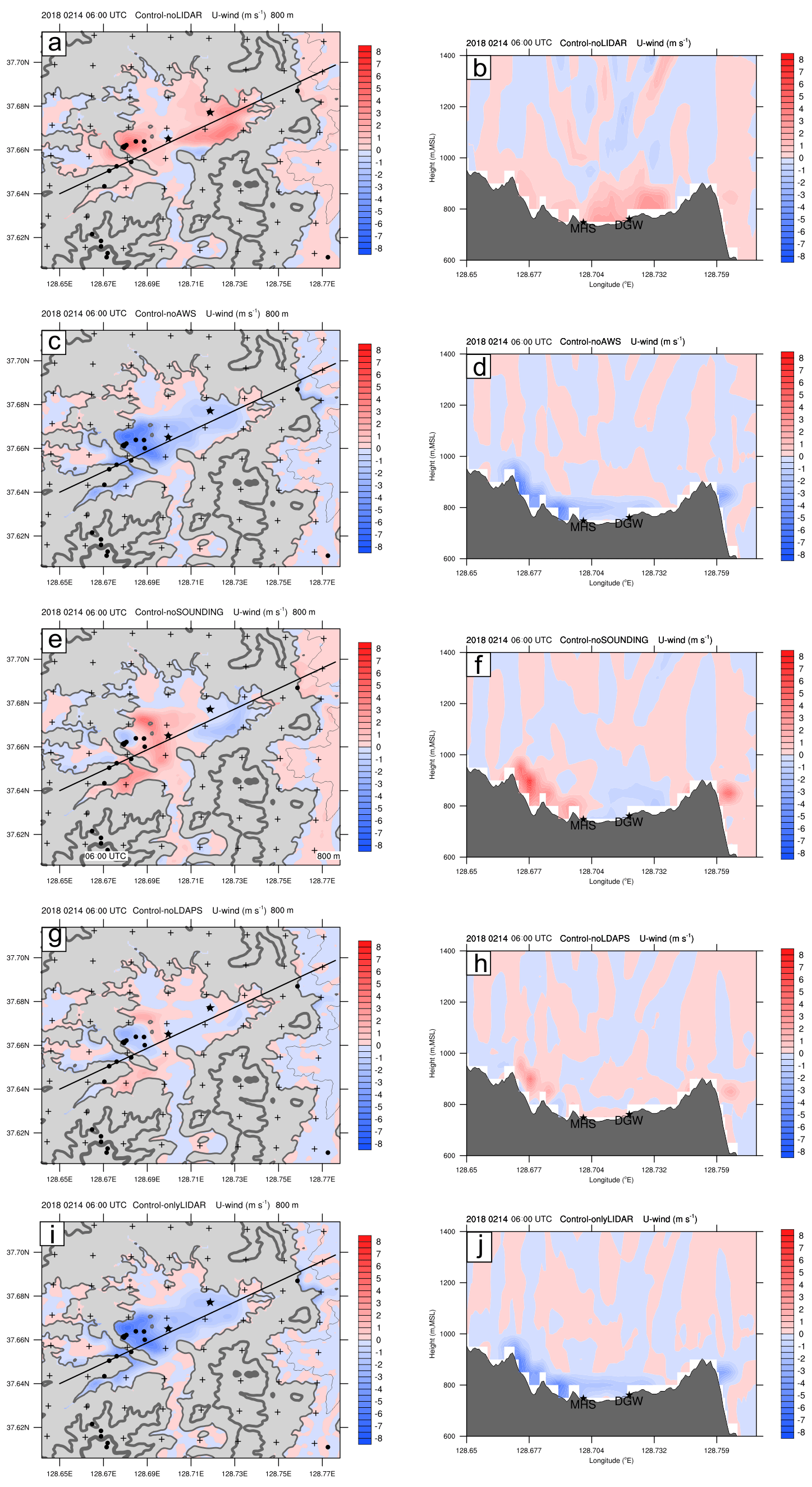
Figure 12(a) The discrepancies in horizontal u-component winds between the control run and A-1 at 800 m a.m.s.l. at 06:00 UTC on 14 February 2018. (b) The same as panel (a) but for the vertical section along the black line in panel (a). Panels (c) and (d) are the same as panels (a) and (b) but for A-2. Panels (e) and (f) are the same as panels (a) and (b) but for A-3. Panels (g) and (h) are the same as panels (a) and (b) but for A-4. Panels (i) and (j) are the same as panels (a) and (b) but for A-5.
Figure 12a reveals the discrepancies in horizontal u-component winds at 800 m a.m.s.l. as the A-1 is subtracted from the control run. This result reflects the impacts of lidar observations on the u-component winds in the WISSDOM synthesis. The most significant contribution from the lidar observations is the high wind speed existing near the DGW site in a relatively narrow valley. The mechanisms of the accelerated wind speed due to the channeling effect in this local area were verified by our previous study (Tsai et al., 2022). The lidar observations also contributed to the high wind speed in another area near the western side of the MHS site (37.66∘ N, 128.68∘ E). Based on the analysis in the vertical cross section of u-component winds in A-1 (Fig. 12b), the lidar observations significantly affected the high wind speed only in the lower levels (below ∼900 m a.m.s.l.) but not in the higher levels. Lidar observations provided sufficient coverage only for lower levels and not higher levels (see Fig. 4).
The impacts of the AWSs cause negative values in the u-component winds in most areas at 800 m a.m.s.l. in A-2 (Fig. 12c), especially in the western areas of the MHS site. Negative contributions of the u-component winds produced by the AWS observations were restricted near the surface, and the low wind speed area was extended to ∼100 m above the surface (Fig. 12d). The contributions of the u-component winds from the sounding observations were weak near the DGW sounding site in A-3 (Fig. 12e and f). The impacts of u-component winds from the LDAPS datasets were rather smaller in most of the analysis area in A-4 (Fig. 12g and h). Relatively weak winds were presented near the surface from the results of A-5 (Fig. 12i and j). These results reflect that the additional constraints play crucial roles, especially at lower layers. Furthermore, it is implied that the winds can be reasonably retrieved when additional constraints are set in the modified version of WISSDOM.
Averaged discrepancies in derived 3D winds for each vertical level in the entire domain are shown in Fig. 13a. These results summarize a series of sensitivity tests if the WISSDOM synthesis lacks certain data inputs (i.e., A-1 to A-5 in Experiment A) for derived u-, v-, and w-component winds in the test domain. Overall, the maximum absolute value of averaged discrepancies in Experiment A are smaller than approximately 0.5 m s−1, which are the discrepancies in the u-component winds for A-1 and A-2 located at 800 m a.m.s.l. Except for these values, the values of the derived u-, v-, and w-component winds for A-1 to A-2 are approximately smaller than 0.2 m s−1 from the surface up to the top in the test domain. Based on the results of A-5, relatively stronger values of derived u-component winds (exceeding −0.4 m s−1 at lower layers) can be obtained using settings like in the old version of WISSDOM. The wind speed can be better modulated in modified version of WISSDOM when the Doppler lidar observations are adopted.
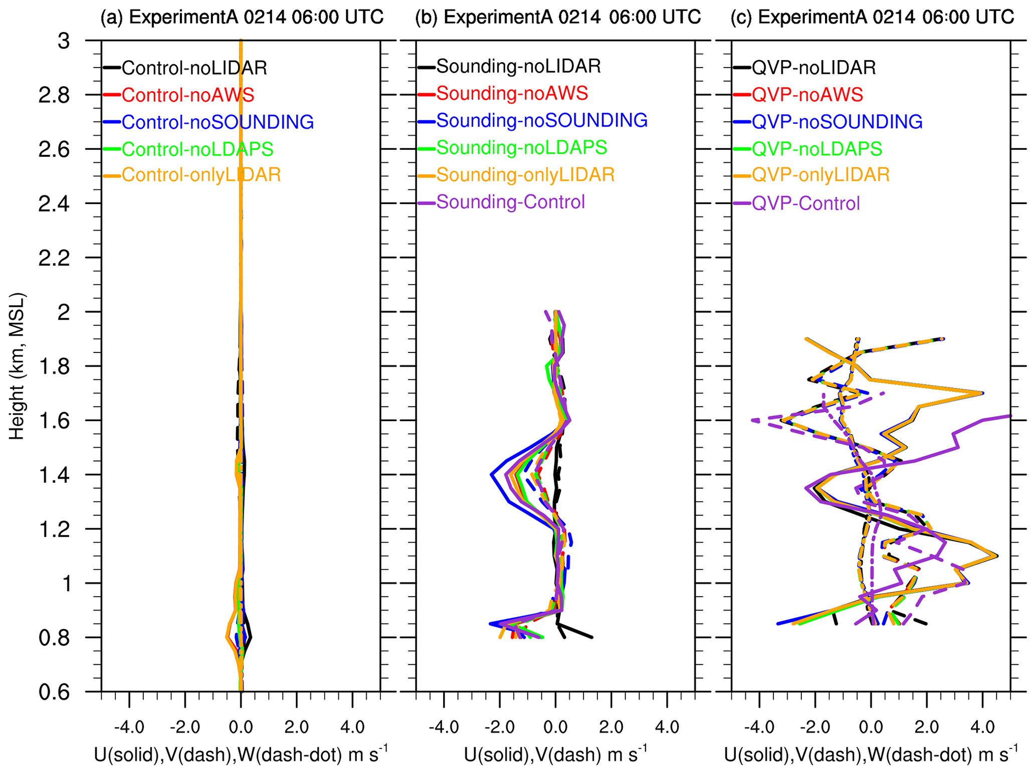
Figure 13(a) Vertical profiles of averaged discrepancies in 3D winds for each design in Experiment A at 06:00 UTC on 14 February 2018. The averaged discrepancies in u-, v-, and w-component winds were plotted by solid, dashed, and dashed-dotted lines, and the black, red, blue, green, and orange lines indicate A-1, A-2, A-3, A-4, and A-5, respectively. (b) The same as panel (a) but for the discrepancies between sounding observations, u- and v-component winds, and control run (purple lines). (c) The same as panel (b) but for the discrepancies between QVP and w-component winds.
In addition, the discrepancies in derived 3D winds between sounding observations and QVP were also examined along the sounding tracks (Fig. 13b) and above the DGW site (Fig. 13c). Sounding observations played an essential role in the derived winds along its tracks. The maximum discrepancies in u-component winds are exceeded by approximately −2 m s−1 and v-component winds by approximately −1 m s−1 if the WISSDOM synthesis lacks sounding observations. However, small discrepancies (nearly 0 m s−1) presented themselves when the sounding data were implemented, and the lidar was not implemented at all levels in A-1. The peaks in the discrepancies manifested the potential impacts from the lidar and AWSs. This may result from lidar and AWSs having higher data coverage at ∼1.4 and 0.8 km a.m.s.l., respectively (see Fig. 4). The discrepancies between sounding observations and the control run in u- and v-component winds reveal relatively smaller values than the A-3 but similar to the other designs (purple lines in Fig. 13b). The maximum discrepancies between the derived winds and the QVP winds are approximately −4 and 4 m s−1 associated with u- and v-component winds, and −1 and 0 to the w-component winds. Generally, the results reveal similar trends in A-1 to A-5, implying that all the inputs in the WISSDOM synthesis are equally significant against the QVP. The QVP winds and control run discrepancies in u- and v-component winds show similar values for all designs, but relatively small values can be obtained in w-component winds (purple lines in Fig. 13c). In summary, the results of this experiment (see Fig. 13) show that the lidar, sounding, and AWS data are more critical inputs than the LDAPS in modified WISSDOM. Therefore, it will be beneficial if various inputs can be included in the synthesis.
5.2 Radius of influence (RI) and vertical extension for the AWSs (Experiment B)
Experiment B was performed to check the discrepancies in 3D winds between the control run and the different settings of RI and VE with the AWS observations. Because the average distance is approximately 0.1 to 2 km between each AWS site, there were five designs (B-1 to B-5) in Experiment B with ranges of RI (VE) between 0.5 km (50 %) and 2 km (90 %). The details are shown in Table 4. The horizontal u-component winds at 800 m a.m.s.l. and the vertical structure of Experiment B at one time step (06:00 UTC on 14 February 2018) are shown in Fig. 14. An unusual circular area with positive discrepancies around the MHS site was depicted in B-1 (Fig. 14a and b), which may have been produced by the insufficient RI distance and VE (the circular artifact is removed when increasing VE to 90 %). Relatively smaller RI and VE values can only include relatively less wind information if the distances are large between each AWS. Enlarging the RI and VE is required to appropriately include more wind information from the AWS observations. Figure 14c and d show the results of B-2 as VE reached 90 %. Although the unusual circle vanished, there were discontinuities with negative values near the northern and southern areas of the MHS site and positive areas surrounding the AWS (37.66∘ N, 128.68∘ E). The setting of B-3 was similar to that of the control run except that the VE was 50 %. The discrepancies were relatively small, albeit dense AWSs contributed even smaller negative values in the western areas of the MHS sites (Fig. 14g and h). Obviously, positive discrepancies appeared near the northern and southern areas of the MHS site in B-4 and B-5 (Fig. 14g–j). The impacts of the AWSs with various settings (B-1 to B-5) on the discrepancies in u-component winds were both restricted near the surface, even with a larger RI and high VE.
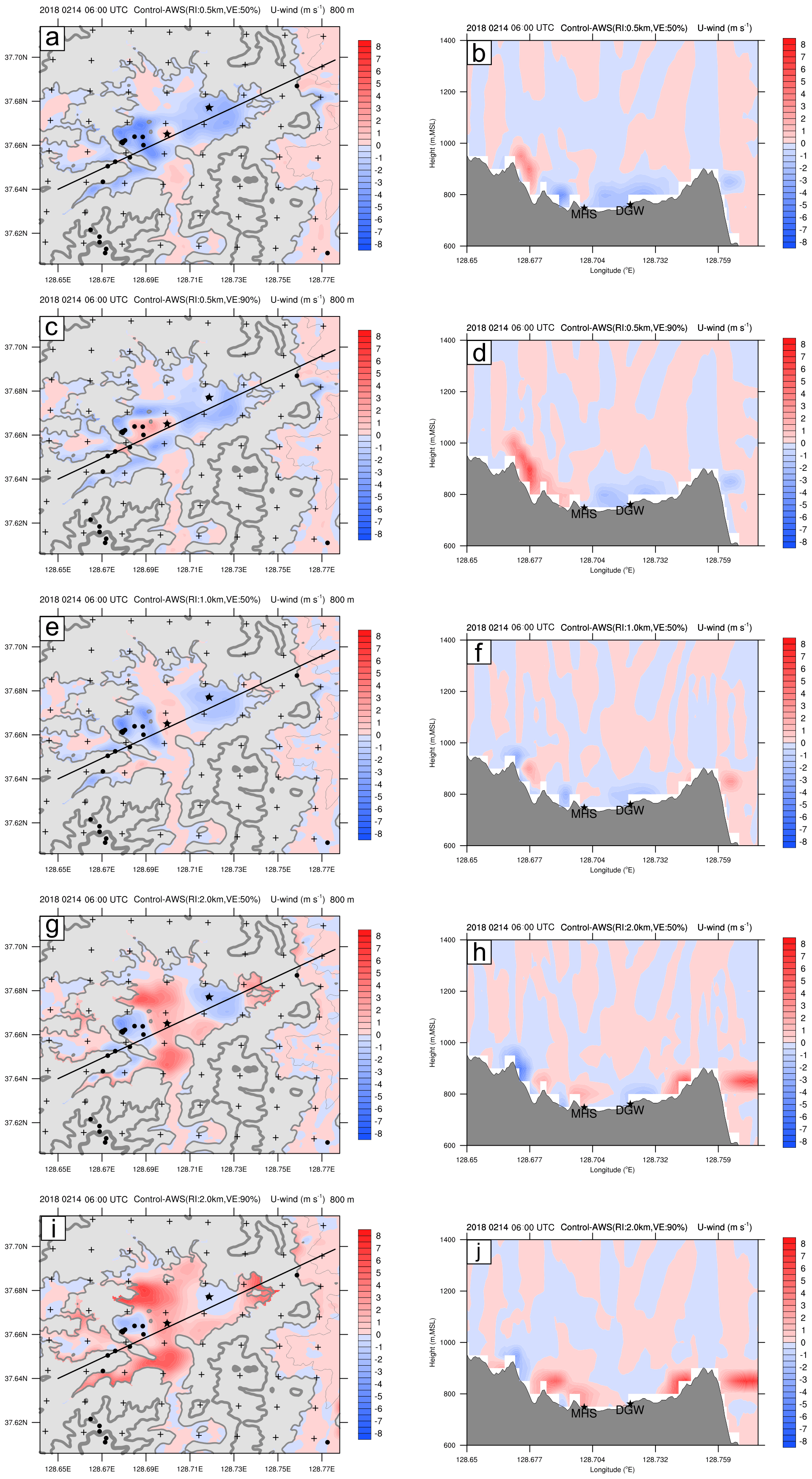
Figure 14The same as Fig. 12 but for B-1 (a, b). Panels (c) and (d) are the same as panels (a) and (b) but for B-2. Panels (e) and (f) are the same as panels (a) and (b) but for B-3. Panels (g) and (h) are the same as panels (a) and (b) but for B-4. Panels (i) and (j) are the same as panels (a) and (b) but for B-5.
Figure 15a shows the vertical profiles of averaged discrepancies in derived 3D winds in Experiment B. This figure summarizes the results of sensitivity testing with different settings of the RI and VE in WISSDOM (i.e., B-1 to B-5 in Experiment B, shown in Table 4) for derived u-, v-, and w-component winds in the test domain. The maximum discrepancies in u-component winds in B-1, B-2, and B-3 were quite small at only 0.4, 0.3, and 0.2 m s−1, respectively. Nevertheless, the maximum discrepancies in u-component winds for B-4 and B-5 were larger than 0.6 m s−1 and even exceeded ∼1 m s−1. Although the discrepancies in the u-component winds in B-1 were small, the discrepancies in the v-component winds in B-1 reveal unusual patterns, with larger positive values at ∼1100 m a.m.s.l. and negative values at ∼1800 m a.m.s.l. (dashed black line in Fig. 15a), the possible reason is that the minimizations of the cost function are not converged well because relatively few and weak v-component winds were included in B-1. Except for this value, the maximum discrepancies in v-component winds were small for B-2 to B-5, and the maximum discrepancies in w-component winds were also small for all of Experiment B. Note that B-3 always has the smallest discrepancies in the derived 3D winds because the setting is quite similar to the control run. Figure 15b and c show the discrepancies in derived 3D winds between the sounding observations, QVP, and control run. Their patterns are similar to A-1 to A-5 (see Fig. 13b and c) except there were relatively larger values of u-component (v-component) winds at lower layers (approximately −3 and 1 m s−1) in B-1 (Fig. 15b). The v-component winds also presented larger values (exceeded ∼3 m s−1) below ∼1.2 km a.m.s.l. compared with the QVP (Fig. 15c). The conclusions indicate that the moderate setting (i.e., RI is 1 km) would be helpful to obtain smaller differences with the control run, sounding observations, and the QVP in this case. On the other hand, the limited setting in experiment B (i.e., B-1) was not suitable. In addition, the wind directions and speed should be dominated by terrain, and the implementation of AWS data is crucial for the modified WISSDOM synthesis, especially in the lower layers.

5.3 Different weighting coefficients for the constraints (Experiment C)
Experiment C was designed to check the discrepancies in the derived u-component winds between the control run and experimental runs with different weighting coefficients for each constraint related to the AWS, lidar, and LDAPS (corresponding to C-1, C-2, and C-3 in Table 4). Originally, the weighting coefficients for the AWS and lidar observations were set to 106, and the value was 103 for the LDAPS dataset (i.e., control run; Table 1). The results of Experiment C show significant negative discrepancies in u-component winds near the surface in C-1, especially in the areas next to the AWS (37.66∘ N, 128.68∘ E). The discrepancies for C-1 (Fig. 16a and b) and C-2 (Fig. 16c and d) are similar to those for A-2 (Fig. 12c and d) and A-1 (Fig. 12a and b), respectively. The inputs of the AWS and lidar both contributed relatively weak impacts to the WISSDOM synthesis when the weighting coefficient was set to 103. Irrational patterns were depicted when the weighting coefficient of LDAPS inputs increased to 106, and larger and positive discrepancies were crowded into most areas in the valley (i.e., C-3; Fig. 16e). Larger and positive discrepancies existed only near the surface, and there were negative discrepancies between approximately 1000 and 1400 m (Fig. 16f). Significant differences often exist between the observations and reanalysis dataset due to the differing spatiotemporal resolutions. The results of scenario C-3 do not converge well because there was a relatively more significant gradient between each input as their weighting coefficients were set to be the same (i.e., 106). In this way, the effects of poor convergences might be amplified with the AWS and lidar observations along the sounding tracks. This may be a possible reason that artificial signals existed over the DGW site in scenario C-3.
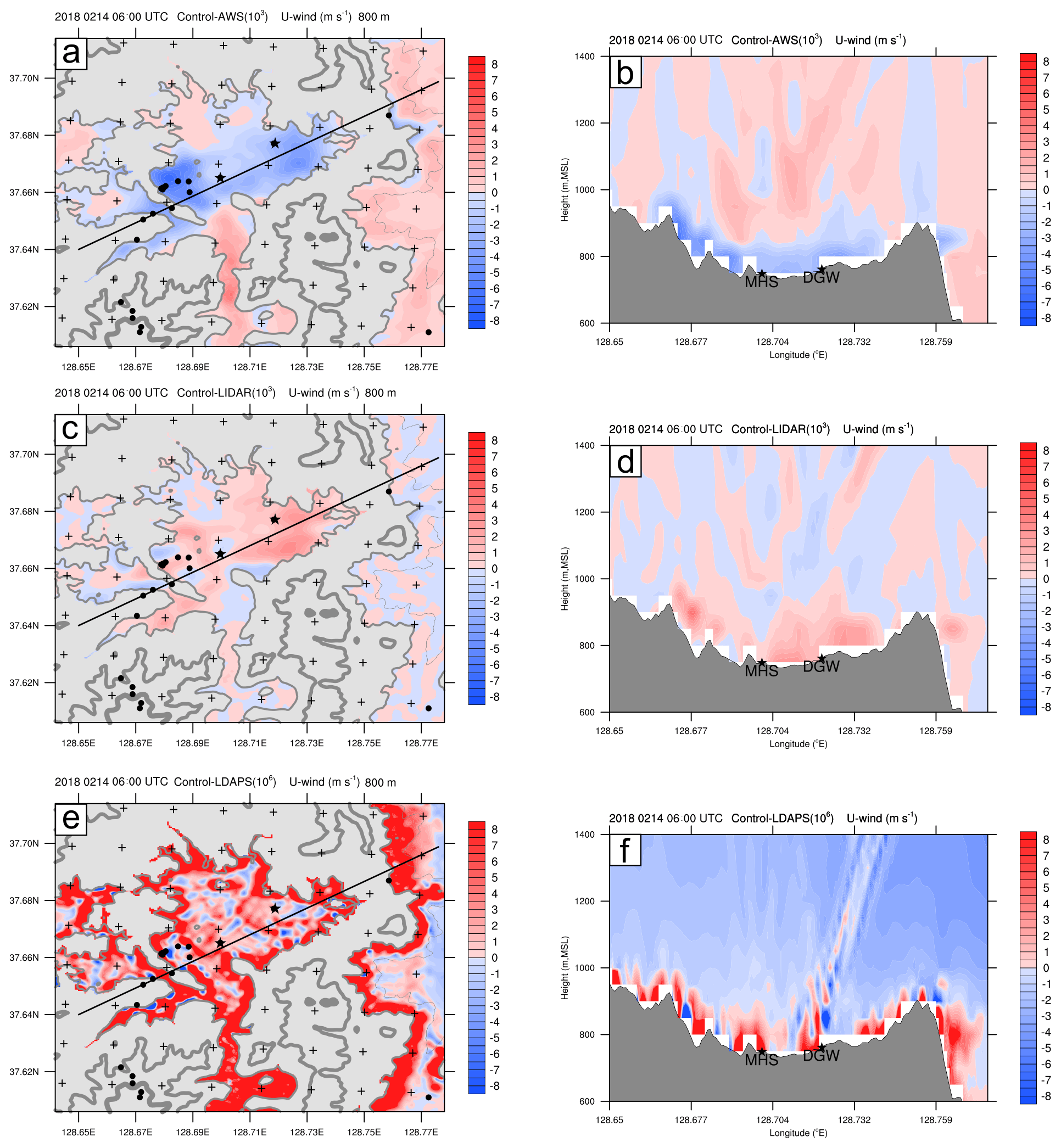
Figure 16The same as Fig. 12 but for C-1 (a, b). Panels (c) and (d) are the same as panels (a) and (b) but for C-2. Panels (e) and (f) are the same as panels (a) and (b) but for C-3.
The vertical profiles of averaged discrepancies in derived 3D winds in Experiment C are shown in Fig. 17a. Absolute values of the discrepancies in the u-, v-, and w-component winds are smaller than 1 m s−1 except for the discrepancies in the v-component winds with low weighting of the AWS observations (i.e., C-1) and the discrepancies in the u- and v-component winds with the high weighted LDAPS (i.e., C-3). The discrepancies in the v-component winds in C-1 exceeded −5 m s−1 at ∼1100 m a.m.s.l. and were larger than −15 m s−1 above 2600 m a.m.s.l. These unreasonable characteristics are also shown as the discrepancies in the v-component winds in B-1 (see Fig. 15a). The discrepancies in the u- and v-component winds in C-3 are 15 and 4 m s−1, respectively, in the layers between 700 and 900 m a.m.s.l. Alternative positive and negative discrepancies in the range of −3 to 3 m s−1 for the u-component winds in C-3 were found above 1000 m a.m.s.l.

The discrepancies between the derived 3D winds in Experiment C and the sounding observations and QVP were also examined. Compared to the sounding observations, more significant discrepancies in the u- and v-component winds (exceeding ∼20 m s−1) can be obtained when reducing the weighting coefficients of the AWS and increasing the weighting coefficients of the LDAPS data (Fig. 17b). However, the impacts of lidar against the QVP are shown; their discrepancies are in the range of −1 to 2 m s−1 for the u-component winds in C-2 (Fig. 17c). The discrepancies between sounding observations, the QVP winds, and the control run were more minor than all designs in Experiment C (purple lines in Fig. 17b and c). The conclusions reveal that the weighting coefficients of the AWS and LDAPS are significantly sensitive to the derived winds, and the lidar is moderately sensitive to the retrieved winds. Therefore, it is better for the weighting coefficients of LDAPS and the AWS to be 103 and 106 in this case.
A modified WISSDOM synthesis scheme was developed to derive high-quality 3D winds under clear-air conditions. The main difference from the original version is that multiple lidar observations were used in the modified version, replacing radar data. High-resolution 3D winds (50 m horizontally and vertically) were first derived in the modified WISSDOM scheme. In addition, the wind information was separated from the background in the modified version. Therefore, all available datasets were included as one of the constraints in the cost function in this study. The data implementation and the detailed principles of the modified WISSDOM were also elaborated. This modified WISSDOM scheme was performed over the TMR to retrieve 3D winds during a strong wind event during ICE-POP 2018. The performance was evaluated via a series of sensitivity tests and compared with conventional observations.
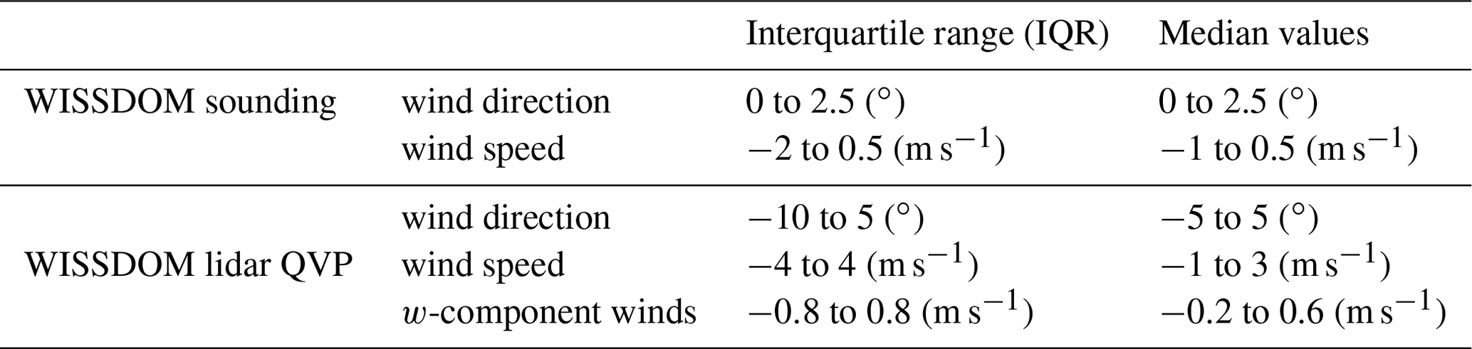
The intercomparisons of horizontal winds during the entire research period reveal a relatively high correlation coefficient between the optimal results of WISSDOM synthesis and sounding's u-component (v-component) winds exceeding 0.97 (0.87) at the DGW site. Furthermore, the average bias is −0.78 m s−1 (0.09 m s−1), and the RMSD is 1.77 m s−1 (1.65 m s−1) for the u-component (v-component) winds. The intercomparisons of 3D winds between the WISSDOM synthesis and lidar QVP also showed a higher correlation coefficient (0.84) for u-component winds, but a relatively smaller correlation coefficient remained at 0.35 for v-component winds in this strong wind event. The average bias (RMSD) of u-component winds is 2.83 m s−1 (3.69 m s−1), and the average bias and RMSD of v-component winds are 2.26 and 2.92 m s−1, respectively (see Table 2). Chen (2019) analyzed the correlations between 3D winds derived from radar and observations in several typhoon cases; the mean correlation coefficient ranged from 0.56 to 0.86, and the RMSD was between 1.13 and 1.74 m s−1. Compared to their results, only u-component winds have relatively higher correlation coefficients, but the RMSD values are slightly higher in this study, which may have been caused by the high variability in westerly winds associated with the moving LPS. The statistical error results of the winds between the optimal results of WISSDOM synthesis and observations show the good performance of the retrieved 3D winds in this strong wind event (Table 3). Generally, the median values of wind directions are within ∼10∘. Compared with lidar QVP (sounding observations) above the DGW site, the median values of the wind speed are approximately −1 to 3 m s−1 (−1 to 0.5 m s−1), and the vertical velocity is within −0.2 to 0.6 m s−1; the IQR of wind directions is −10 to 5∘ (0–2.5∘), the wind speed is approximately −4 to 4 m s−1 (−1 to 3 m s−1), and the vertical velocity is −0.8 to 0.8 m s−1. The summaries of the correlation coefficients, average bias, the RMSD, and the range of statistical errors are shown in the schematic diagrams of Fig. 18a and b.

Figure 18Schematic diagrams for the results of intercomparisons on (a) the correlation coefficients (R, histograms), the average bias (marked as diamonds), and the RMSD (marked as asterisks). (b) The ranges of statistic error for the IQR (red boxes) and median values (blue boxes). The wind directions, wind speed, and w-component winds are denoted as Wd, Ws, and W, respectively.
A control run (see the basic setting in Table 1) was set to explore the importance of acquired observation datasets, various distances of RI, VE from the AWS observations, and the weighting coefficient for each constraint (i.e., Experiments A–C; Table 4). The results of Experiment A show that the lidar and AWSs play critical roles in the derived horizontal winds, and the lidars (AWSs) provided positive (negative) contributions in stronger (weaker) wind speeds near the surface. The sounding and the LDAPS had a relatively more minimal impact on the derived horizontal winds from the WISSDOM synthesis. In Experiment B, minor discrepancies in 3D winds were depicted when the RI (VE) was set to 1 km (50 %), which indicated that the optimal setting of the RI is 1 km. However, there were larger discrepancies in 3D winds (from −0.4 to ∼1 m s−1) when the RI was set at 0.5 and 2 km, and the VE was set between 50 % and 90 % (see Fig. 15). In Experiment C, significant discrepancies in 3D winds appeared by decreasing (rising) the weighting coefficient from the AWS observations (LDAPS datasets). Relatively reasonable winds can be derived with the setting of 1 km in RI and 90 % in VE over complex terrain (i.e., the same setting as the control run). These sensitivity tests will help verify the impacts against various scenarios and observational references in this area.
This study demonstrated that reasonable patterns of 3D winds were derived by the modified WISSDOM synthesis scheme in a strong wind event. Reasonable winds can be retrieved from modified WISSDOM with sufficient coverage from the data, a moderate weighting function, and appropriate implementation from different datasets. In the future, many cases are required to check the performance of this modified WISSDOM scheme with different synoptic weather systems under clear-air conditions in different seasons. In addition, knowing the detailed kinematic fields will help us to identify where the flow accelerates/decelerates over complex terrain. Thus, the possible mechanisms of extremely strong winds in South Korea will be well documented through combinations with derived dynamic fields (Tsai et al., 2018, 2022), thermodynamic fields (Liou et al., 2019), observations, and simulations. The detailed wind structures can be well documented for any meteorological phenomena in clear-air conditions (e.g., land–sea breezes, micro-downbursts, nonprecipitation low-pressure systems) via a modified version of WISSDOM. It also has broad applications in site surveys of wind turbines, wind energy, monitoring wildfires, outdoor sports in mountain ranges, and aviation security.
The scanning Doppler lidar, AWS, and sounding data used in this study are available through Zenodo: https://doi.org/10.5281/zenodo.6537507 (Tsai, 2022). The LDAPS dataset is freely available from the KMA website (https://data.kma.go.kr/cmmn/selectMemberAgree.do, last access: 8 February 2023; KMA, 2023).
This work was made possible by contributions from all authors. CLT and GWL: conceptualization; CLT, YCL, and KK: methodology; CLT, YCL, and KK: software; KK, YCL, and GWL: validation; CLT and KK: formal analysis; CLT and GWL: investigation; CLT: writing – original draft preparation; GWL, YCL, and KK: writing – review and editing; CLT: visualization; GWL: supervision; GWL: funding acquisition. All authors have read and agreed to the published version of the manuscript.
The contact author has declared that none of the authors has any competing interests.
Publisher's note: Copernicus Publications remains neutral with regard to jurisdictional claims in published maps and institutional affiliations.
This article is part of the special issue “Winter weather research in complex terrain during ICE-POP 2018 (International Collaborative Experiments for PyeongChang 2018 Olympic and Paralympic winter games) (ACP/AMT/GMD inter-journal SI)”. It is not associated with a conference.
This work was supported by the National Research Foundation of Korea (NRF) grant funded by the Korea government (MSIT) and the Korea Meteorological Administration Research and Development Program.
This research has been supported by the National Research Foundation of Korea (NRF; grant no. 2021R1A4A1032646) and the Korea Meteorological Administration (grant no. KMI2022-00310).
This paper was edited by Alexis Berne and reviewed by two anonymous referees.
Armijo, L.: A theory for the determination of wind and precipitation velocities with Doppler radars, J. Atmos. Sci., 26, 570–573, 1969.
Bell, M. M., Montgomery, M. T., and Emanuel, K. A.: Air–sea enthalpy and momentum exchange at major hurricane wind speeds observed during CBLAST, J. Atmos. Sci., 69, 3197–3222, https://doi.org/10.1175/JAS-D-11-0276.1, 2012.
Bell, T. M., Klein, P., Wildmann, N., and Menke, R.: Analysis of flow in complex terrain using multi-Doppler lidar retrievals, Atmos. Meas. Tech., 13, 1357–1371, https://doi.org/10.5194/amt-13-1357-2020, 2020.
Browning, K. A. and Wexler, R.: The Determination of Kinematic Properties of a Wind Field Using Doppler Radar, J. Appl. Meteorol., 7, 105–113, https://doi.org/10.1175/1520-0450(1968)007<0105:TDOKPO>2.0.CO;2, 1968.
Cha, T.-Y. and Bell, M. M.: Comparison of single-Doppler and multiple-Doppler wind retrievals in Hurricane Matthew (2016), Atmos. Meas. Tech., 14, 3523–3539, https://doi.org/10.5194/amt-14-3523-2021, 2021.
Chen, Y.-A.: Verification of multiple-Doppler-radar derived vertical velocity using profiler data and high resolution examination over complex terrain, MS thesis, National Central University, 91 pp., 2019.
Choi, D., Hwang, Y., and Lee, Y. H.: Observing Sensitivity Experiment Based on Convective Scale Model for Upper-air Observation Data on GISANG 1 (KMA Research Vessel) in Summer 2018, Atmosphere, 30, 17–30, 2020 (Korean with English abstract).
Choukulkar, A., Brewer, W. A., Sandberg, S. P., Weickmann, A., Bonin, T. A., Hardesty, R. M., Lundquist, J. K., Delgado, R., Iungo, G. V., Ashton, R., Debnath, M., Bianco, L., Wilczak, J. M., Oncley, S., and Wolfe, D.: Evaluation of single and multiple Doppler lidar techniques to measure complex flow during the XPIA field campaign, Atmos. Meas. Tech., 10, 247–264, https://doi.org/10.5194/amt-10-247-2017, 2017.
Colle, B. A. and Mass, C. F.: High-Resolution Observations and Numerical Simulations of Easterly Gap Flow through the Strait of Juan de Fuca on 9–10 December 1995, Mon. Weather Rev., 128, 2398–2422, 2000.
Cressman, G. P.: An operational objective analysis system. Mon. Weather Rev., 87, 367–374, 1959.
Gao, J., Droegemeier, K. K., Gong, J., and Xu, Q.: A method for retrieving mean horizontal wind profiles from single-Doppler radar observations contaminated by aliasing, Mon. Weather Rev., 132, 1399–1409, https://doi.org/10.1175/1520-0493-132.6.1399, 2004.
Hill, M., R. Calhoun, H. J. S. F., Wieser, A., Dornbrack, A., Weissmann, M., Mayr, G., and Newsom, R.: Coplanar Doppler lidar retrieval of rotors from T-REX, J. Atmos. Sci., 67, 713–729, 2010.
Jou, B. J.-D., Lee, W.-C., Liu, S.-P., and Kao, Y.-C.: Generalized VTD retrieval of atmospheric vortex kinematic structure. Part I: Formulation and error analysis, Mon. Weather Rev., 136, 995–1012, https://doi.org/10.1175/2007MWR2116.1, 2008.
Kim, D.-J., Kang, G., Kim, D.-Y., and Kim, J.-J.: Characteristics of LDAPS-Predicted Surface Wind Speed and Temperature at Automated Weather Stations with Different Surrounding Land Cover and Topography in Korea, Atmosphere, 11, 1224, https://doi.org/10.3390/atmos11111224, 2020.
Kim, J., Sharman, R. D., Benjamin, S. G., Brown, J. M., Park, S., and Klemp, J. B.: Improvement of Mountain Wave Turbulence Forecast in the NOAA's Rapid Refresh (RAP) Model with Hybrid Vertical Coordinate System, Weather Forecast., 34, 773–780, https://doi.org/10.1175/WAF-D-18-0187.1, 2019.
Kim, K., Lyu, G., Baek, S., Shin, K., and Lee, G.: Retrieval and Accuracy Evaluation of Horizontal Winds from Doppler Lidars during ICE-POP 2018, Atmos., 32, 163–178, https://doi.org/10.14191/ATMOS.2022.32.2.163, 2022.
KMA (Korea Meteorological Administration): Meteorological Data Open Portal, KMA, https://data.kma.go.kr/cmmn/selectMemberAgree.do, last access: 8 February 2023.
Lee, J., Seo, J., Baik, J., Park, S., and Han, B.: A Numerical Study of Windstorms in the Lee of the Taebaek Mountains, South Korea: Characteristics and Generation Mechanisms, Atmosphere, 11, 431, https://doi.org/10.3390/atmos11040431, 2020.
Lee, J.-T., Ko, K.-Y., Lee, D.-I., You, C.-H., and Liou, Y.-C.: Enhancement of orographic precipitation in Jeju Island during the passage of Typhoon Khanun (2012), Atmos. Res., 201, 1245–1254, https://doi.org/10.1016/j.atmosres.2017.10.013, 2017.
Lee, J.-T., Ko, K.-Y., Lee, D.-I., You, C.-H., and Liou, Y.-C.: Enhancement of orographic precipitation in Jeju Island during the passage of Typhoon Khanun (2012), Atmos. Res., 201, 58–71, https://doi.org/10.1016/j.atmosres.2017.10.013, 2018.
Lee, W.-C., Marks Jr., F. D., and Carbone, R. E.: Velocity track display – A technique to extract real-time tropical cyclone circulations using a single airborne Doppler radar, J. Atmos. Ocean. Tech., 11, 337–356, https://doi.org/10.1175/1520-0426(1994)011<0337:VTDTTE>2.0.CO;2, 1994.
Lee, W.-C., Jou, B. J.-D., Chang, P.-L., and Deng, S.-M.: Tropical cyclone kinematic structure derived from single-Doppler radar observations. Part I: Interpretation of Doppler velocity patterns and the GBVTD technique, Mon. Weather Rev., 127, 2419–2439, https://doi.org/10.1175/1520-0493(1999)127<2419:TCKSRF>2.0.CO;2, 1999.
Liou, Y. and Chang, Y.: A Variational Multiple–Doppler Radar Three-Dimensional Wind Synthesis Method and Its Impacts on Thermodynamic Retrieval, Mon. Weather Rev., 137, 3992–4010, https://doi.org/10.1175/2009MWR2980.1, 2009.
Liou, Y., Chang, S., and Sun, J.: An Application of the Immersed Boundary Method for Recovering the Three-Dimensional Wind Fields over Complex Terrain Using Multiple-Doppler Radar Data, Mon. Weather Rev., 140, 1603–1619, https://doi.org/10.1175/MWR-D-11-00151.1, 2012.
Liou, Y., Chen Wang, T., Tsai, Y., Tang, Y., Lin, P., and Lee, Y.: Structure of precipitating systems over Taiwan's complex terrain during Typhoon Morakot (2009) as revealed by weather radar and rain gauge observations, J. Hydrol., 506, 14–25, https://doi.org/10.1016/j.jhydrol.2012.09.004, 2013.
Liou, Y., Chiou, J., Chen, W., and Yu, H.: Improving the Model Convective Storm Quantitative Precipitation Nowcasting by Assimilating State Variables Retrieved from Multiple-Doppler Radar Observations, Mon. Weather Rev., 142, 4017–4035, https://doi.org/10.1175/MWR-D-13-00315.1, 2014.
Liou, Y., Chen Wang, T., and Huang, P.: The Inland Eyewall Reintensification of Typhoon Fanapi (2010) Documented from an Observational Perspective Using Multiple-Doppler Radar and Surface Measurements, Mon. Weather Rev., 144, 241–261, https://doi.org/10.1175/MWR-D-15-0136.1, 2016.
Liou, Y.-C., Wang, T.-C. C., Lee, W.-C., and Chang, Y.-J.: The retrieval of asymmetric tropical cyclone structures using Doppler radar simulations and observations with the extended GBVTD technique, Mon. Weather Rev., 134, 1140–1160, https://doi.org/10.1175/MWR3107.1, 2006.
Liou, Y. C., Yang, P. C., and Wang, W. Y.: Thermodynamic recovery of the pressure and temperature fields over complex terrain using wind fields derived by multiple-Doppler radar synthesis, Mon. Weather Rev., 147, 3843–3857, https://doi.org/10.1175/MWR-D-19-0059.1, 2019.
Mass, C. F. and Ovens, D.: The Northern California Wildfires of 8–9 October 2017: The Role of a Major Downslope Wind Event, B. Am. Meteorol. Soc., 100, 235–256, https://doi.org/10.1175/BAMS-D-18-0037.1, 2019.
Mohr, C. G. and Miller, L. J.: CEDRIC – A software package for Cartesian Space Editing, Synthesis, and Display of Radar Fields under Interactive Control, Preprints, 21st Conf. on Radar Meteorology, Edmonton, AB, Canada, Amer. Meteor. Soc., 569–574, 1983.
North, K. W., Oue, M., Kollias, P., Giangrande, S. E., Collis, S. M., and Potvin, C. K.: Vertical air motion retrievals in deep convective clouds using the ARM scanning radar network in Oklahoma during MC3E, Atmos. Meas. Tech., 10, 2785–2806, https://doi.org/10.5194/amt-10-2785-2017, 2017.
Oue, M., Kollias, P., Shapiro, A., Tatarevic, A., and Matsui, T.: Investigation of observational error sources in multi-Doppler-radar three-dimensional variational vertical air motion retrievals, Atmos. Meas. Tech., 12, 1999–2018, https://doi.org/10.5194/amt-12-1999-2019, 2019.
Park, J.-R., Kim, J.-H., Shin, Y., Kim, S.-H., Chun, H.-Y., Jang, W., Tsai, C.-L., and Lee, G.: A numerical simulation of a strong windstorm event in the Taebaek Mountain Region in Korea during the ICE-POP 2018, Atmos. Res., 272, 106158, https://doi.org/10.1016/j.atmosres.2022.106158, 2022.
Päschke, E., Leinweber, R., and Lehmann, V.: An assessment of the performance of a 1.5 µm Doppler lidar for operational vertical wind profiling based on a 1-year trial, Atmos. Meas. Tech., 8, 2251–2266, https://doi.org/10.5194/amt-8-2251-2015, 2015.
Reed, T. R.: GAP WINDS OF THE STRAIT OF JUAN DE FUCA, Mon. Weather Rev., 59, 373–376, https://doi.org/10.1175/1520-0493(1931)59<373:GWOTSO>2.0.CO;2, 1931.
Ryzhkov, A., Zhang, P., Reeves, H., Kumjian, M., Tschallener, T., Trömel, S., and Simmer, C.: Quasi-Vertical Profiles–A New Way to Look at Polarimetric Radar Data, J. Atmos. Ocean. Tech., 33, 551–562, https://doi.org/10.1175/JTECH-D-15-0020.1, 2016.
Tsai, C.-L.: Data for WISSDOM Synthesis in A Strong Wind Event 13-14 Feb. 2018, Zenodo [data set], https://doi.org/10.5281/zenodo.6537507, 2022.
Tsai, C.-L., Kim, K., Liou, Y., Lee, G., and Yu, C.: Impacts of Topography on Airflow and Precipitation in the Pyeongchang Area Seen from Multiple-Doppler Radar Observations, Mon. Weather Rev., 146, 3401–3424, https://doi.org/10.1175/MWR-D-17-0394.1, 2018.
Tsai, C.-L., Kim, K., Liou, Y.-C., Kim, J.-H., Lee, Y., and Lee, G.: Orographic-induced strong wind associated with a low-pressure system under clear-air condition during ICE-POP 2018, J. Geophys. Res.-Atmos., 127, e2021JD036418, https://doi.org/10.1029/2021JD036418, 2022.
Tseng, Y. and Ferziger, J.: A ghost-cell immersed boundary method for flow in complex geometry, J. Comput. Phys., 192, 593–623, https://doi.org/10.1016/j.jcp.2003.07.024, 2003.
Yu, C.-K. and Bond, N. A.: Airborne Doppler observations of a cold front in the vicinity of Vancouver Island, Mon. Weather Rev., 130, 2692–2708, https://doi.org/10.1175/1520-0493(2000)128<1577:ADOOAL>2.0.CO;2, 2002.
Yu, C.-K. and Jou, B. J.-D.: Radar observations of diurnally forced, offshore convective lines along the southeastern coast of Taiwan, Mon. Weather Rev., 133, 1613–1636, https://doi.org/10.1175/MWR2937.1, 2005.
Yu, C.-K. and Tsai, C.-L.: Surface Pressure Features of Landfalling Typhoon Rainbands and Their Possible Causes, J. Atmos. Sci., 67, 2893–2911, https://doi.org/10.1175/2010JAS3312.1, 2010.
Yu, C.-K. and Tsai, C.-L.: Structural and surface features of arc-shaped radar echoes along an outer tropical cyclone rainband, J. Atmos. Sci., 70, 56–72, https://doi.org/10.1175/JAS-D-12-090.1, 2013.
Yu, C.-K. and Tsai, C.-L.: Structural changes of an outer tropical cyclone rain band encountering the topography of northern Taiwan, Q. J. Roy. Meteor. Soc., 143, 1107–1122, https://doi.org/10.1002/qj.2994, 2017.
Yu, C.-K., Cheng, L.-W., Wu, C.-C., and Tsai, C.-L.: Outer Tropical Cyclone Rainbands Associated with Typhoon Matmo (2014), Mon. Weather Rev., 148, 2935–2952, https://doi.org/10.1175/MWR-D-20-0054.1, 2020.
- Abstract
- Introduction
- Methodology
- Data processing with a strong wind event
- Control run and the accuracy of WISSDOM
- Sensitivity test with various datasets, data implementation, and weighting coefficients
- Conclusion
- Code and data availability
- Author contributions
- Competing interests
- Disclaimer
- Special issue statement
- Acknowledgements
- Financial support
- Review statement
- References