the Creative Commons Attribution 4.0 License.
the Creative Commons Attribution 4.0 License.
 | 21 Feb 2023
Performance of AIRS ozone retrieval over the central Himalayas: use of ozonesonde and other satellite datasets
Prajjwal Rawat
Evan Fishbein
Pradeep K. Thapliyal
Rajesh Kumar
Piyush Bhardwaj
Aditya Jaiswal
Sugriva N. Tiwari
Sethuraman Venkataramani
Shyam Lal
Data from 242 ozonesondes launched from ARIES, Nainital (29.40∘ N, 79.50∘ E; 1793 m elevation), are used to evaluate the Atmospheric Infrared Sounder (AIRS) version 6 ozone profiles and total column ozone during the period 2011–2017 over the central Himalayas. The AIRS ozone products are analysed in terms of retrieval sensitivity, retrieval biases/errors, and ability to retrieve the natural variability in columnar ozone, which has not been done so far from the Himalayan region, having complex topography. For a direct comparison, averaging kernel information is used to account for the sensitivity difference between the AIRS and ozonesonde data. We show that AIRS has more minor differences from ozonesondes in the lower and middle troposphere and stratosphere with nominal underestimations of less than 20 %. However, in the upper troposphere and lower stratosphere (UTLS), we observe a considerable overestimation of the magnitude, as high as 102 %. The weighted statistical error analysis of AIRS ozone shows a higher positive bias and standard deviation in the upper troposphere of about 65 % and 25 %, respectively. Similarly to AIRS, the Infrared Atmospheric Sounding Interferometer (IASI) and the Cross-track Infrared Sounder (CrIS) are also able to produce ozone peak altitudes and gradients successfully. However, the statistical errors are again higher in the UTLS region, which are likely related to larger variability in ozone, lower ozone partial pressure, and inadequate retrieval information on the surface parameters. Furthermore, AIRS fails to capture the monthly variation in the total column ozone, with a strong bimodal variation, unlike unimodal variation seen in ozonesondes and the Ozone Monitoring Instrument (OMI). In contrast, the UTLS and the tropospheric ozone columns are in reasonable agreement. Increases in the ozone values of 5 %–20 % after biomass burning and during events of downward transport are captured well by AIRS. Ozone radiative forcing (RF) derived from total column ozone using ozonesonde data (4.86 mW m−2) matches well with OMI (4.04 mW m−2), while significant RF underestimation is seen in AIRS (2.96 mW m−2). The fragile and complex landscapes of the Himalayas are more sensitive to global climate change, and establishing such biases and error analysis of space-borne sensors will help us study the long-term trends and estimate accurate radiative budgets.
- Article
(3971 KB) - Full-text XML
-
Supplement
(2070 KB) - BibTeX
- EndNote


Atmospheric ozone is an essential trace gas that plays a crucial role in the atmospheric oxidizing chemistry, air quality, and earth's radiative budget. The stratospheric ozone absorbs harmful solar ultraviolet radiation and protects biological life on earth, whereas tropospheric ozone, being a secondary air pollutant (e.g. Pierce et al., 2009; Monks et al., 2015; Lelieveld et al., 2018) and greenhouse gas, contributes to global warming and can harm human health and crops when present in higher concentrations near the surface (Fishman et al., 1979; Ebi and McGregor, 2008; Lal et al., 2017). Different radiative forcing of ozone from the stratosphere (cooling) to the troposphere (heating) (Lacis et al., 1990; Wang et al., 1993; Forster et al., 2007; Hegglin et al., 2015) demonstrates its potential importance as an atmospheric climate gas (Shindell et al., 2012; Thornhill et al., 2021). Hence, information regarding precise long-term variability in global ozone distribution is vital for better characterizing atmospheric chemistry and global climate changes (Kim and Newchurch, 1996; Myhre et al., 2017).
In recent decades, observations of ozone from space-borne sensors (microwave limb sounding, UV–VIS, and IR) have become an increasingly robust tool for global and higher temporal monitoring (e.g. Bhartia et al., 1996; Foret et al., 2014). This increases our ability to analyse various influences of human activities on the atmospheric chemical composition, including ozone; study their long-term impact on climate (Fishman and Larsen, 1987; Tarasick et al., 2019; Thornhill et al., 2021); and estimate reliable radiative budgets (Hauglustaine and Brasseur, 2001; Gauss et al., 2003; Aghedo et al., 2011). However, the space-based sensors are indirect and measure the atmospheric composition based upon specific algorithms utilizing radiative transfer models and a priori information. Hence, the retrieval outputs need to be evaluated with certain reference instruments for establishing the credibility and better utilization of space-borne data.
The Himalayas, a complex terrain region, has the largest abundance of ice sheets outside polar regions that impact global and regional radiative budgets and climate pervasively (e.g. Lawrence and Lelieveld, 2010; Cristofanelli et al., 2014). Very sparse in situ and ground-based observations in this region, along with inadequate information on the surface parameters, make it difficult to retrieve the atmospheric composition from space-borne instruments. This is because the ozone weighting function, a measure of the retrieval sensitivity and a fundamental retrieval component, depends upon various atmospheric parameters like surface temperature, surface emissivity, and terrain height (Rodgers, 1976, 1990; Bai et al., 2014), which is not uniform over the footprint size of the Atmospheric Infrared Sounder (AIRS; ∼ 13 km × 13 km) in the Himalayas. Usually, the ozone weighting function has a shorter integrating path over the elevated terrain regions, which follows a smaller weighting function and provides less sensitivity and more errors in the final retrievals (Coheur et al., 2005; Bai et al., 2014).
The Atmospheric Infrared Sounder (AIRS) on board the Aqua satellite has been providing reliable vertical profiles of ozone, temperature, water vapour, and other trace gases globally twice a day since 2002. Numerous validation studies of AIRS-retrieved ozone have been carried out for different versions since it started operating (2002). For example, Bian et al. (2007) studied AIRS version 4 over Beijing and discussed the potential agreements (within 10 %) between AIRS and ozonesonde (GPSO3) ozone, particularly in the upper-troposphere and lower-stratosphere (UTLS) region with the capability of AIRS to identify various stratosphere–troposphere exchange (STE) and transient convective events. Similarly, a study over Boulder, USA, and Lauder, New Zealand, by Monahan et al. (2007) using a similar AIRS version showed that, despite the larger biases in the lower and middle tropospheric region, the retrieval algorithm captures the ozone variability very effectively with a positive correlation of more than 70 %. However, that study suggested a need for tropopause-adjusted coordinates in the a priori profiles. Both these studies (Bian et al., 2007; Monahan et al., 2007) show larger biases in AIRS ozone in the lower and middle tropospheric regions; however, shifts in retrieval biases and errors were seen towards the UTLS region in version 5 (Divakarla et al., 2008), apart from significant improvements in the lower troposphere. The retrieval methodology has also changed significantly between V4 and V5. Version 4 or earlier used regression retrieval as the first guess in physical retrieval, while later versions used a climatology-based first guess for the physical retrieval based on other works (McPeters et al., 2007). Also, radiative transfer models, selected channel sets, and clarified quality indicators have been modified and improved in all successive versions.
The AIRS ozone retrieval in V5 has improved significantly with retrieval biases and root mean square error (RMSE) less than 5 % and 20 %, respectively (Divakarla et al., 2008), over the tropical regions. However, there has not been much discussion or many studies of the assessment for AIRS ozone over the Himalayas' complex terrain, where retrieval is expected to be erroneous due to large surface variability within its footprint. Also, most of the previous studies (Bian et al., 2007; Divakarla et al., 2008; Pittman et al., 2009) did not utilize the averaging kernel information of AIRS that is vital for satellite evaluation. Recently, ozonesonde observations have also been utilized to evaluate the total and tropospheric ozone column from various satellite retrievals over the Andes Mountains. This study shows nominal differences between satellite and ozonesonde for the total column ozone, while the tropospheric ozone column shows a difference of up to 32.5 % (Cazorla and Herrera, 2022). Such evaluation studies, along with the present analysis, comprehend the possible differences between satellite and truth observations and advise towards the trustworthiness of satellite data over the complex mountain regions.
Specifically, here, the evaluation of AIRS version 6, which entirely depends upon the infrared (IR) observations after the failure of the advanced microwave sounding unit (AMSU) sensor, is presented in terms of statistical analysis and ability to retrieve the natural variability in ozone at various altitudes over the central Himalayan region using in situ ozonesonde observations convolved with AIRS averaging kernels. Additionally, the present study assessed the AIRS retrieval algorithm using the Infrared Atmospheric Sounding Interferometer (IASI) and the Cross-track Infrared Sounder (CrIS) radiance information for 1 year. AIRS columnar ozone (i.e. total, UTLS, and tropospheric columns) is also assessed with ozonesonde, Ozone Monitoring Instrument (OMI), and Microwave Limb Sounder (MLS) observations. AIRS has a long-term dataset for ozone and meteorological parameters, and establishing such biases and error analysis is essential to make meaningful use of its data to characterize the Himalayan atmosphere, study the trends and radiative budgets, and perform the model evaluation and data assimilation over this region.
2.1 Data description
2.1.1 AIRS
The Atmospheric Infrared Sounder (AIRS) on board the Aqua satellite, in a sun-synchronous polar orbit at 705 km altitude, is a hyperspectral thermal infrared grating spectrometer with equatorial crossings at ∼ 13:30 local time (LT). It is a nadir scanning sensor that was deployed in orbit on 4 May 2002. AIRS, along with its partner microwave instrument, the Advanced Microwave Sounding Unit (AMSU-A), represents the most advanced atmospheric sounding system placed in space using cutting-edge infrared and microwave technologies. These instruments together observe the global energy cycles, water cycles, climate variations, and greenhouse gases; however, after the AMSU failure, the retrieval now mostly depends upon the AIRS IR observations. The AIRS infrared spectrometer acquires 2378 spectral samples at resolutions () ranging from 1086 to 1570 cm−1 in three bands: 3.74 to 4.61, 6.20 to 8.22, and 8.8 to 15.4 µm (Fishbein et al., 2003; Pagano et al., 2003). The independent channels of AIRS permit the retrieval of various atmospheric states and constituents depending upon their corresponding spectral response, even in the presence of a 90 % cloud fraction (Susskind et al., 2003; Maddy and Barnet, 2008). In this study, we have used the Level 2 Support physical products of AIRS (AIRS2SUP). The AIRS2SUP files (∼ 240 granules d−1) possess extra information over the standard AIRS files, e.g. information on averaging kernel and degree of freedom, including vertical profiles at 100 pressure levels against just 28 in the standard product.
The support product profiles contain 100 levels between 1100 and 0.016 mbar. While it has a higher vertical resolution, the vertical information content is no greater than the standard product. The information on averaging kernels and degrees of freedom (DOFs) is utilized to understand the retrieved products more comprehensively. The DOFs of ozone, a measure of significant eigenfunctions used in the AIRS retrieval, have an average value of 1.36 over the tropical latitude band (Maddy and Barnet, 2008) (Table S1 in the Supplement), while over the balloon-collocated region, an average DOF of 1.62 is observed (Fig. S1). In the present study, the AIRS data are flagged as best quality when the cloud fraction is less than 80 % and the DOFs are greater than 0.04. However, analysis of cloud fraction over our collocated region shows (Fig. S2) that only 7 % of observations during 2011–2017 had a cloud fraction of more than 80 %.
2.1.2 IASI (NOAA/CLASS)
The Infrared Atmospheric Sounding Interferometer (IASI) on board MetOp satellites, with a primary focus on meteorology rather than climate and atmospheric chemistry monitoring, is a nadir-viewing Michelson interferometer (Clerbaux et al., 2007). The first MetOp satellite was launched in October 2006 (MetOp-A), and IASI was declared operational in July 2007. MetOp is a polar sun-synchronous satellite having descend and ascend nodes at 09:30 and 21:30 LT, respectively. IASI measures in the IR part of the electromagnetic (EM) spectrum at a horizontal resolution of 12 km at nadir up to 40 km over a swath width of about 2200 km. IASI covers an infrared spectral range between 3.7 and 15.4 µm with a total of 8461 spectral channels, out of which 53 channels around 9.6 µm are utilized for ozone retrieval. IASI level 2 ozone products provided by NOAA National Environmental Satellite, Data, and Information Service (NESDIS) Center for Satellite Applications and Research (STAR) are used in this study. The IASI (NOAA/CLASS: NOAA Comprehensive Large Array-data Stewardship System) ozone product is retrieved based on the AIRS algorithm and has various quality control (QC) flags (Table S2). Only QC = 0 data which represent a successful IR ozone retrieval are used.
2.1.3 CrIS/ATMS (NUCAPS)
The Cross-track Infrared Sounder (CrIS) and Advanced Technology Microwave Sounder (ATMS) on board the Suomi National Polar-orbiting Partnership (NPP) satellite were launched in 2011 to feature the high-spectral-resolution (“hyperspectral”) observations of earth's atmosphere. The CrIS instrument is an advanced Fourier transform spectrometer with an ascending node at 13:30 LT and flies at a mean altitude of 824 km and performs 14 orbits d−1. It measures high-resolution IR spectra in the spectral range 650–2550 cm−1 with a total of 1305 channels. The ATMS is a microwave sounder with a total of 22 channels ranging from 23 to 183 GHz. These two instruments, CrIS and ATMS, operate in an overlapping field-of-view (FOV) formation, with ATMS FOVs re-sampled to match the location and size of the 3 × 3 CrIS FOVs for retrieval under clear to partly cloudy conditions. Here the NOAA Unique Combined Atmospheric Processing System (NUCAPS) algorithm-based ozone product of CrIS is utilized. The NOAA Unique CrIS/ATMS Processing System is a heritage algorithm developed by the STAR team based on the AIRS retrieval algorithm (Susskind et al., 2003, 2006). The NOAA-implemented NUCAPS algorithm is a modular architecture that was specifically designed to be compatible with multiple instruments. The same retrieval algorithms are currently used to process the AIRS/AMSU suite (operations since 2002), the IASI/AMSU/MHS suite (operational since 2008), and now the CrIS/ATMS suite (approved for operations in January 2013). Here again, various quality controls for retrieved data are provided by the NUCAPS science algorithm team, and we used QC = 0 for smaller discrepancies in our evaluation (Table S2). These research products follow a similar retrieval algorithm as developed by the AIRS science team, which gives us further opportunity to assess the AIRS retrieval algorithm for IASI and CrIS radiances.
2.1.4 Ozonesonde
EN-SCI electrochemical concentration cell (ECC) ozonesondes and GPS radiosondes (iMet) have been launched from the Aryabhatta Research Institute of Observational Sciences (ARIES) (29.4∘ N, 79.5∘ E; 1793 m elevation), Nainital (Fig. 1), a high-altitude site in the central Himalayas, since 2011 (Ojha et al., 2014; Rawat et al., 2020), the only facility in the Himalayan region having regular launchings. The ECC ozonesonde relies on the oxidation reaction of ozone with potassium iodide (KI) solution (Komhyr, 1967; Komhyr et al., 1995) to measure ozone partial pressure in the ambient atmosphere. The typical vertical resolution of the ozonesonde is about 100–150 m and has a precision of better than ±3 %–5 % with an accuracy of about ±5 %–10 % up to 30 km altitude under standard operating procedures (Smit et al., 2007, 2021). The ozonesonde is connected to the iMet radiosonde via a V7 electronic interface, in which the radiosonde consists of GPS, PTU (pressure, temperature, and humidity), and a transmitter to transmit signals to the ground.
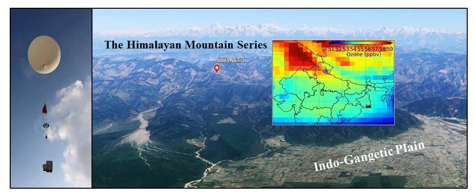
Figure 1Location (red colour circle) of the balloon launching site (© Google Earth, 2021) situated in the Aryabhatta Research Institute of Observational Sciences (ARIES) (29.4∘ N, 79.5∘ E; 1793 m elevation), Nainital, in the central Himalayas. The spatial distribution of ozone (AIRS) at 500 hPa is also shown over northern India, and the location of the site is marked with a blue star. A photo of balloon, together with parachute, unwinder, ozonesonde, and GPS radiosonde, above the observation site is also shown at the left.
The ozonesonde sensor's successful performance is assured before launch (about 3–7 d before launch) as part of advance preparation and during the day of launch by maintaining and reviewing the records for background current, pump flow rate, response time, etc. The ozonesonde data quality is further assured by estimating these ECC ozonesondes' total ozone normalization factor with collocated OMI total ozone (Fig. S3). These factors are well within the Assessment of Standard Operating Procedures for Ozonesondes (ASOPOS) recommendation with an average of 1.0 ± 0.04, which implies the reasonable quality of these ozonesondes (Smit et al., 2021). Additionally, ozonesonde observations from the present site have also been utilized in SusKat (Bhardwaj et al., 2018) and StratoClim (Brunamonti et al., 2018) field campaigns and in other studies (Ojha et al., 2014). Further, owing to higher accuracy and in situ measurement, ozonesondes have been widely used worldwide for satellite and model validation (Monahan et al., 2007; Divakarla et al., 2008; Kumar et al., 2012a, b; Dufour et al., 2012; Verstraeten et al., 2013; Boynard et al., 2016; Rawat et al., 2020). Both the ascending and descending data were recorded by ozonesonde; however, due to time lag in descending records, only ascending data are utilized (Lal et al., 2013, 2014; Ojha et al., 2014). The data are collected at the interval of about 10 m, which is averaged over 100 m interval using a 3σ filter that removes the outlier values (Srivastava et al., 2015; Naja et al., 2016).
2.1.5 Other auxiliary data
Additionally, collocated and concurrent OMI and MLS observations are also used to study the tropospheric ozone, UTLS, and total column ozone due to their reasonable sensitivity and well-validated retrievals (Veefkind et al., 2006; Ziemke et al., 2006; Fadnavis et al., 2014; Wang et al., 2021). The tropospheric ozone column obtained from OMI and MLS is based on the residual method, which depends upon the collocated difference between the MLS stratospheric ozone column and OMI total column ozone and is described in detail by Ziemke et al. (2006). Furthermore, the MLS version 4 data are utilized for the UTLS column above 261 hPa due to their credibility in this range for scientific applications (Livesey et al., 2013; Schwartz et al., 2015). Moreover, for fair statistical analysis between ozonesonde and MLS ozone profiles, Gaussian smoothing is applied to the ozonesonde with full width at half maximum equal to the typical upper-tropospheric vertical resolution (∼ 2–4 km) of MLS (Livesey et al., 2013). The best-quality data of MLS with data flags, i.e. status = even, quality > 0.6, and convergence < 1.18, are utilized (Ziemke et al., 1998; Barré et al., 2012). However, a slightly different collocation criterion of 3∘ × 3∘ grid box and daytime collocation is utilized for MLS in this work due to coarser resolution and to get sufficient matchups.
2.2 Methods of analysis
The balloon launch time is mostly around 12:00 IST (Indian standard time, which is 5.5 h ahead of GMT). The Aqua satellite comes over India around 13:30 and 01:30 IST. Hence for collocation, only noontime (ascending) data (or ±3 h of balloon launch) with 1∘ × 1∘ spatial collocation were chosen in this evaluation. However, for some days, there was no noontime granule in AIRS retrieval (nearly 35 out of a total of 242 soundings), and then we used a loose collocation of ±1 d. However, no significant changes were seen after such flexible collocation. Most of the ozonesondes have burst altitudes near 10 hPa; hence AIRS ozone profiles are evaluated from surface to 10 hPa.
Although suitable collocation criteria have been defined for a fair comparison, the different vertical resolutions of the two datasets (ozonesonde ∼ 100 m and AIRS ∼ 1–5 km) still make the meaningful comparison difficult (Maddy and Barnet, 2008; Verstraeten et al., 2013; Boynard et al., 2016). The difference in vertical resolution and retrieval sensitivity must be accounted for to make a meaningful comparison. Though there is no perfect way to remove the error arising from the different vertical resolutions of the two measurements, still utilizing the averaging kernel smoothing or Gaussian smoothing, the error is minimized. Various groups have used the satellite averaging kernel smoothing to compare satellite and ozonesonde measurements (Zhang et al., 2010; Verstraeten et al., 2013; Boynard et al., 2016, 2018), while Gaussian smoothing (Wang et al., 2020) and broad layer columns (Nalli et al., 2017) are also utilized. In the present analysis, averaging kernel smoothing is utilized (Rodgers and Connor, 2003) and explained with details in Sect. S1.1 in the Supplement. Generally, the contribution of ozone or any other trace gas towards emission/absorption of IR radiation in the radiative transfer equation depends on the exponent of layer-integrated column amounts (Maddy and Barnet, 2008). Hence logarithmic changes in layer column density are more linear than absolute changes. So logarithmic smoothing is utilized in the present study as follows:
where Xest, Xsonde, and X0 are smooth ozonesonde or ozonesonde (AK), true ozonesonde, and first-guess (ML climatology) profiles, respectively. Knowing the nature of convolution from Eq. (1), it can be observed that the ozonesonde (AK) or smooth ozonesonde will have more weights towards a priori profiles when satellite retrieval is poor or AKs approach zero values.
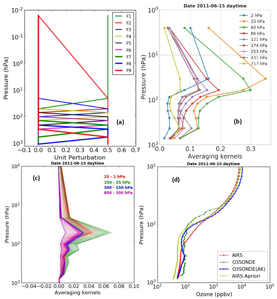
Figure 2(a) Nine trapezoid functions used for ozone retrieval in AIRS-V6. (b) AIRS ozone averaging kernel matrix over Nainital at nine vertical grid levels. (c) Calculated AIRS averaging kernel matrices at 100 RTA grids after applying the trapezoid function. (d) An example of ozone profiles using different datasets for 15 June 2011 over the observation site.
More details on the calculation of averaging kernels, ozone vertices (Table S3), and trapezoid matrix can be found in the AIRS documents (AIRS/AMSU/HSB Version 6 Level 2 Product Levels, Layers and Trapezoids) and in available literature (Maddy and Barnet, 2008; Irion et al., 2018). A typical averaging kernel matrix and other parameters are shown in Fig. 2. Figure 2a shows a typical trapezoid matrix, Fig. 2b shows the averaging kernels at nine pressure levels, Fig. 2c shows constructed averaging kernels at 100 radiative transfer algorithm (RTA) layers, and Fig. 2d shows an example of the different ozone profiles convolved with AKs on 15 June 2011 over the observation site.
Furthermore, the error analysis for AIRS retrieval with interpolated and smoothed ozonesonde is based on Nalli et al. (2013, 2017). Bias, root mean squared error (RMSE), and standard deviation (SD) are studied at various RTA vertical levels from the surface to 10 hPa over the Himalayan region. We have used the W2 weight factor in statistical analysis as suggested by another sounder's science team (Nalli et al., 2013, 2017) and explained in Sect. S1.2.
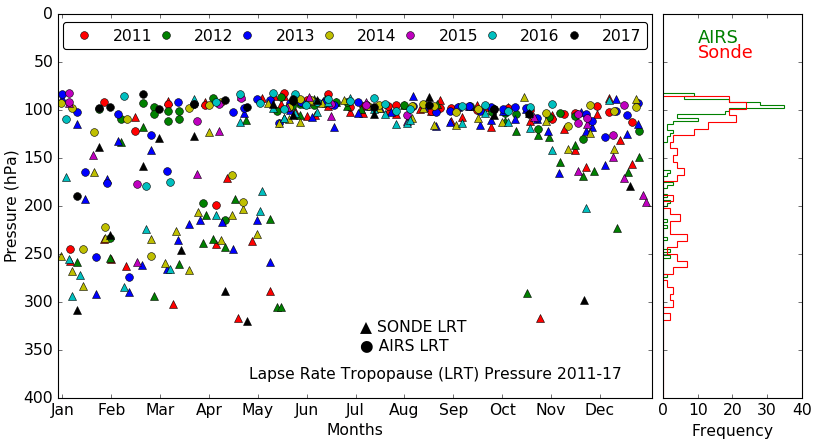
Figure 3Lapse rate tropopause pressure monthly variation from balloon-borne and AIRS observations and respective frequency distributions during 2011–2017.
Additionally, the total column ozone (TCO) from ozonesondes is calculated by integrating the ozone mixing ratio from the surface to burst altitude and then adding residual ozone above burst altitude. Here the residual ozone is obtained from satellite-derived balloon-burst climatology (BBC) (McPeters and Labow, 2012; Stauffer et al., 2022), and the discrete integration is explained in Sect. S1.3. Similarly, the tropospheric column is calculated by integrating ozone from the surface to the lapse rate tropopause (LRT), and the UTLS column is calculated between 400 and 70 hPa (Bian et al., 2007). The tropopause height from balloon-borne observations is estimated using the lapse rate method, and the AIRS-derived tropopause is used and shown in Fig. 3. In addition, the tropospheric ozone column from OMI and MLS observations is also utilized due to its reliable data (Hudson and Thompson, 1998; Ziemke et al., 2006).
3.1 Ozone distribution along balloon trajectory: ozonesonde and AIRS
The distributions of ozone along the balloon tracks obtained using all ozone sounding data during four seasons are shown in Fig. 4. The nearest swath of AIRS ozone observations is interpolated to the balloon locations and altitudes. Altitude variations in the balloon along longitude are shown in Fig. S4. The balloons drift by a very long distance during winter, followed by autumn and spring. During these seasons, balloons often reach Nepal also. The wind reversal took place during the summer monsoon when the balloon drifts towards Indo-Gangetic Plain (IGP) regions (Fig. 4). The distributions of ozone from AIRS are more or less similar to the distributions of those from ozonesondes. Here, the ozone variations are reflecting in terms of spatial and vertical distributions. The bias and coefficient of determination (r2) between ozonesonde and AIRS ozone are studied along the longitude and latitude (Figs. S4 and S5). Lower biases (lower than 10 %) and higher r2 are seen in the lower and middle troposphere. The poor correlation (< 0.4) and larger biases of up to 28 % are seen at certain longitudes that are associated with higher altitudes (> 20 km). Around the balloon launch site (Nainital, 79.45∘ E) the highest r2 score of 0.98 and a low bias of 1.4 % are observed, which remain higher (r2) and lower (bias) up to 80∘ E (Fig. S4).
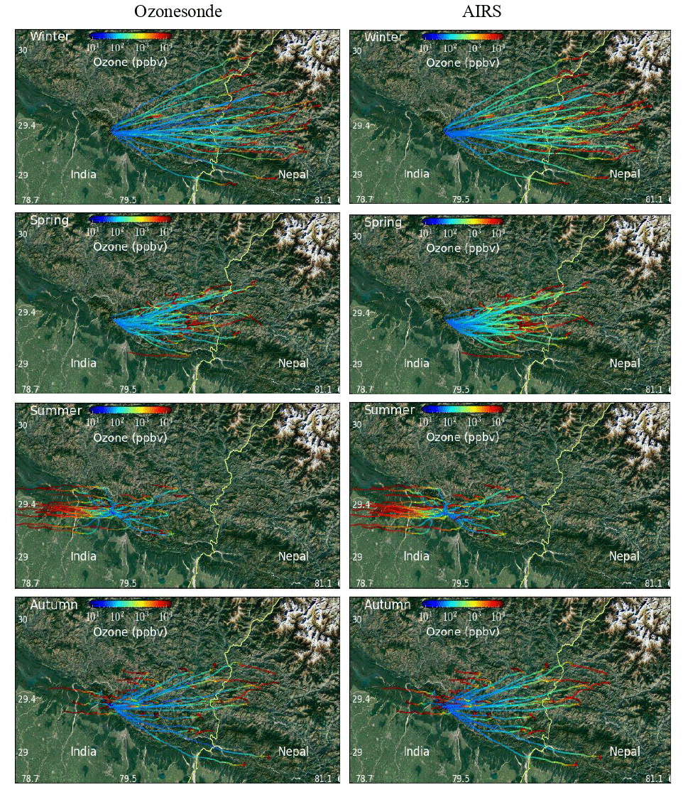
Figure 4Spatial distribution of ozone using all ozone soundings (left) launched from ARIES, Nainital, India (© Google Earth, 2021), along with the balloon trajectories. Ozone spatial distribution from AIRS (right), following the balloon tracks, is also shown. It can be seen that the balloon reaches Nepal many times in the autumn and winter seasons.
3.2 Ozone soundings and AIRS ozone profiles
Figure 5 shows the average monthly ozone profiles for collocated observations of ozonesonde and AIRS during 7-year periods. The ozonesondes convolved with AIRS averaging kernels (ozonesonde – AK) and AIRS a priori profiles are also compared. The value of percentage difference between ozonesonde (AK) and AIRS ozone at 706, 617, 496, 103, 29, and 14 hPa altitudes are shown in Fig. 5, and the zoomed variations in the lower tropospheric ozone (surface to 200 hPa) are also presented in the insets. AIRS slightly (∼ 10 %) underestimates ozone in the lower troposphere during most of the months, except the summer monsoon (June–August), where an overestimation of up to 20 % is observed. In the middle troposphere, around 300 hPa, an underestimation in the range of 1 %–17 % is seen for all months with an approaching tendency of ozonesonde (AK) towards the true ozonesonde profiles. However, near the tropopause region, AIRS retrievals considerably overestimate ozone by up to 102 %. The overestimation was highest for the winter season (82 %–102 %), followed by the spring and autumn, while it was lowest for the summer-monsoon season (10 %–27 %). In the stratosphere, where the sensitivity of AIRS is higher (Fig. 2c), the ozonesonde and AIRS differences were relatively more minor. Additionally, AIRS retrieval shows an underestimation of 5 %–21 % in this altitude region.
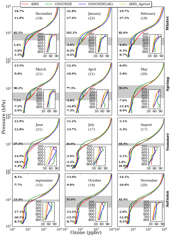
Figure 5Monthly averaged (2011–2017) ozone profiles of ozonesonde, AIRS, ozonesonde (AK), and AIRS a priori profiles over Nainital in the central Himalayas. The percentage differences ((AIRS − ozonesonde (AK)) ozonesonde (AK)) × 100 at 706, 496, 300, 103, 29, and 14.4 hPa are also written at respective altitudes. The standard error corresponding to each profile is also shown with error bars. The number of ozonesondes for different months is written in the brackets, and the grey shaded area shows the tropopause (mean ± σ) from balloon-borne observations.
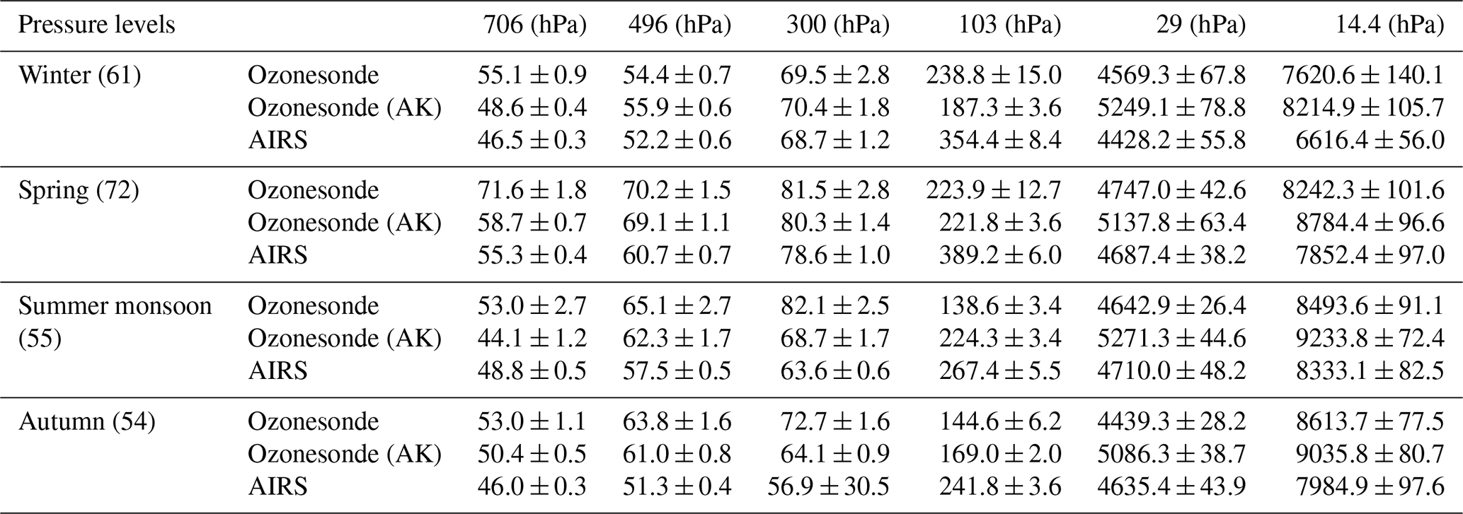
Table 1The mean values and corresponding standard errors in ozone mixing ratio (ppbv) from ozonesonde, ozonesonde (AK), and AIRS over Nainital at six pressure levels and during winter, spring, summer monsoon, and autumn are given. The number of ozonesonde flights during four seasons is mentioned in the brackets.
As expected, the difference between ozonesonde and AIRS is significantly reduced (Table 1) after applying the averaging kernel or accounting for the sensitivity difference. This reduction was more notable for the summer-monsoon period near the tropopause, where the difference reduced from 92 % to 19 %, providing an improvement of 72 %. The improvement was as high as 100 % on a monthly basis. Additionally, relative difference profiles were also analysed for individual soundings, as well for the different seasons (Fig. S6). Greater differences of about 150 % between AIRS and ozonesonde ozone observations were seen in the UTLS region. The greater difference during winter and spring between these observations in the UTLS region could be due to recurring ozone transport via tropopause folding over the observation site. Such events may remain undetected by AIRS due to lower vertical resolution leading to some tropopause folding events being missed at lower altitudes (Fig. 3). However, in the lower troposphere, larger differences between ozonesonde and AIRS during the summer monsoon are seen which are due to low ozone and frequent cloudy conditions leading to poor retrieval. The arrival of cleaner oceanic air during the south-west monsoon (or summer monsoon) brings ozone-poor air and frequent cloudy conditions over northern India that weaken the photochemical ozone production (Naja et al., 2014; Sarangi et al., 2014). Moreover, in the lower troposphere, the limited sensitivity of hyperspectral satellite instruments has a significant contribution from the a priori information, which is also observed for AIRS retrieval (Fig. 5).
Figure 6 shows the yearly time-series analysis of the average ozone mixing ratio at four defined layers, characterizing the middle troposphere (600–300 hPa), the upper troposphere (300–100 hPa), lower stratosphere (100–50 hPa), and middle stratosphere (50–10 hPa). A prominent seasonality was seen in the time series throughout the years, which is quite clear in the upper troposphere (300–100 hPa). The ozone seasonality contrast reflects the influence of the summer-monsoon and winter seasons. The seasonality contrast is similar between AIRS and ozonesonde measurements, while a reversal of ozone seasonality is observed in the middle stratospheric region compared to other layers. The opposite seasonality of the middle stratospheric region is primarily due to dominant circulations, variation in solar radiation, and dynamics. Total column water vapour is also shown in Fig. 6, which shows a tendency of anti-correlation with ozone in the 300–100 hPa region.
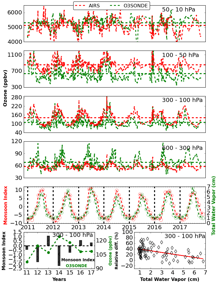
Figure 6Average variations in ozone mixing ratios at four defined layers, characterizing the middle stratosphere (50–10 hPa), the lower stratosphere (100–50 hPa), the upper troposphere (300–100 hPa), and the middle troposphere (600–300 hPa). The dashed horizontal red and green lines show the average ozone mixing ratios in the defined layers from AIRS and ozonesonde, respectively, from 2011 to 2017. The monthly variation in the total column water vapour (cm) along with the monsoon index is also shown. The yearly average ozone from ozonesonde and monsoon index (bar plot) for different years (lowermost left) and the scatter plot of ozone relative difference (%) ((AIRS − O3SONDE) O3SONDE) × 100 with total water vapour (lowermost right) in the upper troposphere (300–100 hPa) are also shown.
We have also estimated the monsoon index by the difference between zonal (U) wind (MERRA-2 reanalysis data) at 850 hPa over the Arabian Sea (5–15∘ N, 40–80∘ E) and over the central Indian landmass (20–30∘ N, 70–90∘ E) as done by Wang et al. (2001).
In general, the positive values of the monsoon index correspond to strong monsoon and negative values to weak monsoon periods (Wang et al., 2001). During the weak monsoon, there is relatively drier air, lower cloud cover, and higher surface temperature compared to the strong monsoon period (Lu et al., 2018). We observed a tendency of lower annual average ozone (from ozonesonde and AIRS measurements) during greater (positive) monsoon index and higher annual average ozone during lower (negative) monsoon index. Lu et al. (2018) have shown an anti-correlation (0.46) of tropospheric ozone with monsoon index over the Indian region. The years 2011, 2012, 2014, and 2015 are classified as weak monsoon years, and relatively higher ozone is seen during these years, whereas for the years 2013, 2016, and 2017, strong monsoon is observed, and average yearly ozone was less during these years (Fig. 6, bottom left). The relative difference in AIRS ozone with ozonesonde in the upper-tropospheric region also shows an anti-correlation (Fig. 6) of 0.17 with total column water vapour. Furthermore, the larger ozone differences between AIRS and ozonesondes are associated with the lower water vapour (Fig. S7), which may be arising due to the influence of ozone-sensitive water vapour (WV) channels in mid-infrared regions. Further, in the middle troposphere (600–300 hPa), a secondary post-monsoon ozone peak is observed, which is suggested to be influenced by the biomass burning (Fig. S8) over northern India that seems to be missing in the AIRS ozone.
In the middle troposphere (600–300 hPa) and lower stratosphere (100–50 hPa), AIRS retrievals show greater differences with respect to ozonesondes, while a nominal difference is observed for the middle troposphere and middle stratosphere (Fig. S7). Furthermore, a systematic increase in standard deviation is also seen with the altitude. The higher standard deviations in the upper-tropospheric and stratospheric regions are mainly due to higher ozone variability associated with stratosphere–troposphere exchange (STE) processes over the Himalayan region (Naja et al., 2016; Bhardwaj et al., 2018).
3.3 Statistical analysis of AIRS ozone profiles
The error analysis of AIRS-retrieved ozone over the Himalayan region is performed with spatio-temporal collocated ozonesonde observations as a reference. The methodology to calculate the root mean square error (RMSE), bias, and standard deviation (SD) is described in Sect. S1.2. W2 weighting statistics are utilized due to abrupt changes in atmospheric ozone with altitude. Here bias and SD between AIRS and ozonesonde are calculated at different RTA layers from surface to 10 hPa. Figure 7 shows the average variation in bias and SD at different RTA layers from surface to 10 hPa over this region. The mean biases between ozonesonde and MLS, a high-vertical-resolution satellite instrument, are also shown in Fig. 7. In general, higher positive biases (∼ 65 %) and SDs (∼ 25 %) in AIRS ozone retrieval are seen in the UTLS region, where MLS agrees well with the ozonesondes. In the lower and middle troposphere, the AIRS ozone retrieval is negatively biased (0 %–25 %), which increases gradually from the surface to higher altitudes (∼ 350 hPa). A negative bias was also seen in the stratosphere of about 15 %. Similarly to the biases, SDs are also smaller in the lower troposphere and stratosphere, with values of nearly 15 %. The higher statistical errors in the upper-tropospheric and the lower-stratospheric region could be due to lower ozone partial pressure and frequent stratospheric to tropospheric transport events over the Himalayas (Rawat et al., 2020; Rawat and Naja, 2021), which introduces errors either after a mismatch of events in AIRS's coarser vertical resolution or due to complex topography. Additionally, the AIRS tropopause frequency distribution shows the limited ability of AIRS to capture deep intrusion events (Fig. 3). Further, AIRS trace-gas retrieval largely depends on successful temperature retrieval and uses temperature retrieval as an input parameter (Maddy and Barnet, 2008). Hence, the temperature retrieval error could also propagate to ozone, and statistical error analysis of AIRS temperature shows relatively higher biases (∼ 2 K) in the upper-tropospheric region (Fig. S9).

Figure 7Statistical error analysis (bias and standard deviation) of AIRS-retrieved ozone with ozonesonde and ozonesonde (AK) for collocated data of 7 years (2011–2017). The bias between collocated data of MLS (261–10 hPa) and ozonesonde over Nainital during 2011–2017 is also shown with the green profile. The grey shaded area shows the tropopause region from balloon-borne radiosonde observations.
The statistical error analysis was more or less similar for both true and smoothed ozonesonde profiles. However, a notable reduction in tropospheric bias and vertical shifts in errors were also observed after applying the averaging kernel matrix to the true ozonesonde throughout the profile. A shift in the error peak is seen from the lower stratosphere to the upper troposphere. This could be due to the higher sensitivity of AIRS retrieval in the lower stratosphere, which would have minimized the error at these particular altitudes. However, in the upper troposphere, the higher contribution of a priori and other factors (i.e. STE) might have resulted in larger biases and errors.
The histogram of differences between AIRS and ozonesonde (AK) is also studied at four defined layers (Fig. S10). AIRS mostly underestimated ozone with a mean bias of 2.4, 9.3, and 39.8 ppbv in 800–600, 600–300, and 100–50 hPa layers, respectively, while in the upper troposphere (300–100 hPa) AIRS overestimated with a mean bias of 43.22 ppbv. Furthermore, distributions of differences are skewed towards the negative values in the lower stratosphere and towards positive values in the upper troposphere. A more symmetric distribution over the negative axis is observed in the middle and lower troposphere. We also studied the correlation profiles for different seasons (Fig. S10, right panel). A strong correlation is seen in the lower and middle troposphere for spring and summer, while there is a poor correlation for winter and autumn. In the lower troposphere, a larger difference between AIRS and ozonesonde (AK) is observed, particularly during summer, with a relatively higher correlation mostly due to the greater concurrence of AIRS a priori profiles with ozonesonde (AK). Whereas in the upper troposphere (300–100 hPa), a larger difference during winter and spring is primarily due to frequent subtropical dynamics, a higher correlation during the winter is mainly contributed from the AIRS retrieval. Furthermore, the analysis of the correlation coefficient between AIRS and ozonesonde over different regions shows a higher correlation in the middle stratosphere (0.95) and lower stratosphere (0.92), followed by the upper troposphere (0.68), lower troposphere (0.62), and middle troposphere (0.47).
3.4 Assessment of AIRS retrieval algorithm with IASI and CrIS radiance
The MetOp IASI and Suomi NPP and CrIS radiance-based ozone products are assessed using ozonesonde data over the central Himalayan region for 1 year (April 2014 to April 2015), utilizing a total of 32 soundings. Here, the IASI- and CrIS-based ozone retrievals are research products provided by NOAA, whose retrieval is based on the AIRS retrieval algorithm and follows a similar averaging kernel matrix (Nalli et al., 2017). For IASI, due to the 09:30 IST ascending nodes (morning overpass in India), a ±6 h loose temporal collocation is used. However, CrIS and AIRS follow the same collocation due to a similar noontime overpass. The IASI, CrIS, and AIRS sensors have 8461, 1305, and 2378 IR channels, respectively. Hence, analysing their satellite ozone products further helps us to assess the AIRS retrieval algorithm for different IR radiances and channel sets.
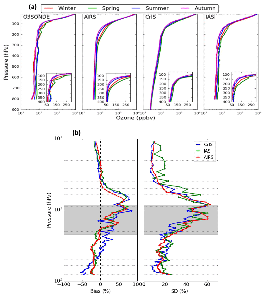
Figure 8(a) Seasonal ozone profiles of three IR satellites (IASI, AIRS, and CrIS) for a smaller sample size (April 2014 to April 2015). The IASI and CrIS products are generated using the AIRS heritage algorithm (NOAA), and only zero quality control flags (QC = 0) of retrievals are used. (b) Statistical error analysis for the ozone retrieved by three IR satellites without applying the averaging kernel information. The grey shaded area shows the tropopause region from balloon-borne observations.
Figure 8a shows the seasonal ozone profiles obtained from three IR satellite sensors along with ozonesondes for a 1-year period. All sensors showed a more or less similar ozone peak altitude and ozone gradient. The estimated ozone peak altitudes for ozonesonde, AIRS, IASI, and CrIS are 11.35, 10, 9.11, and 7.78 hPa, respectively. The estimated average ozone gradients in regions between the tropopause and the gradient peak are 231.5, 199.0, 193.2, and 199.1 ppbv hPa−1 for ozonesonde, AIRS, CrIS, and IASI, respectively.
Moreover, the higher ozone values during spring throughout the troposphere are captured well by all satellite sensors. Higher ozone during spring and winter in the UTLS region is observed well by AIRS and IASI, similarly to ozonesondes, but such features seem to be missing in CrIS ozone retrieval. At the same time, CrIS sensitivity looks relatively low, for which the possible role of the number of channels can be seen. However, IASI and AIRS have effectively captured the ozone seasonal variability.
Figure 8b shows the weighted statistical error analysis of IASI, CrIS, and AIRS ozone retrieval with the true ozonesonde observations. Here, the difference in sensitivity of the two datasets is not accounted for as this section's primary aim is to assess the AIRS-retrieved algorithm using different IR sensor radiances and channel sets. All three space-borne sensors overestimated UTLS ozone by more than 50 %; however, in the stratosphere and lower troposphere, the bias was slightly lower, and it is somewhat underestimated. Similarly to bias, the SDs were also higher in the UTLS region by more than 60 %. A consistent larger difference in the UTLS region for all three IR satellite sensors that share the similar radiative transfer model and retrieval algorithm shows the possible influence of complex topography and the various STE processes in introducing errors in retrieval processes, apart from input a priori data of the retrieval.
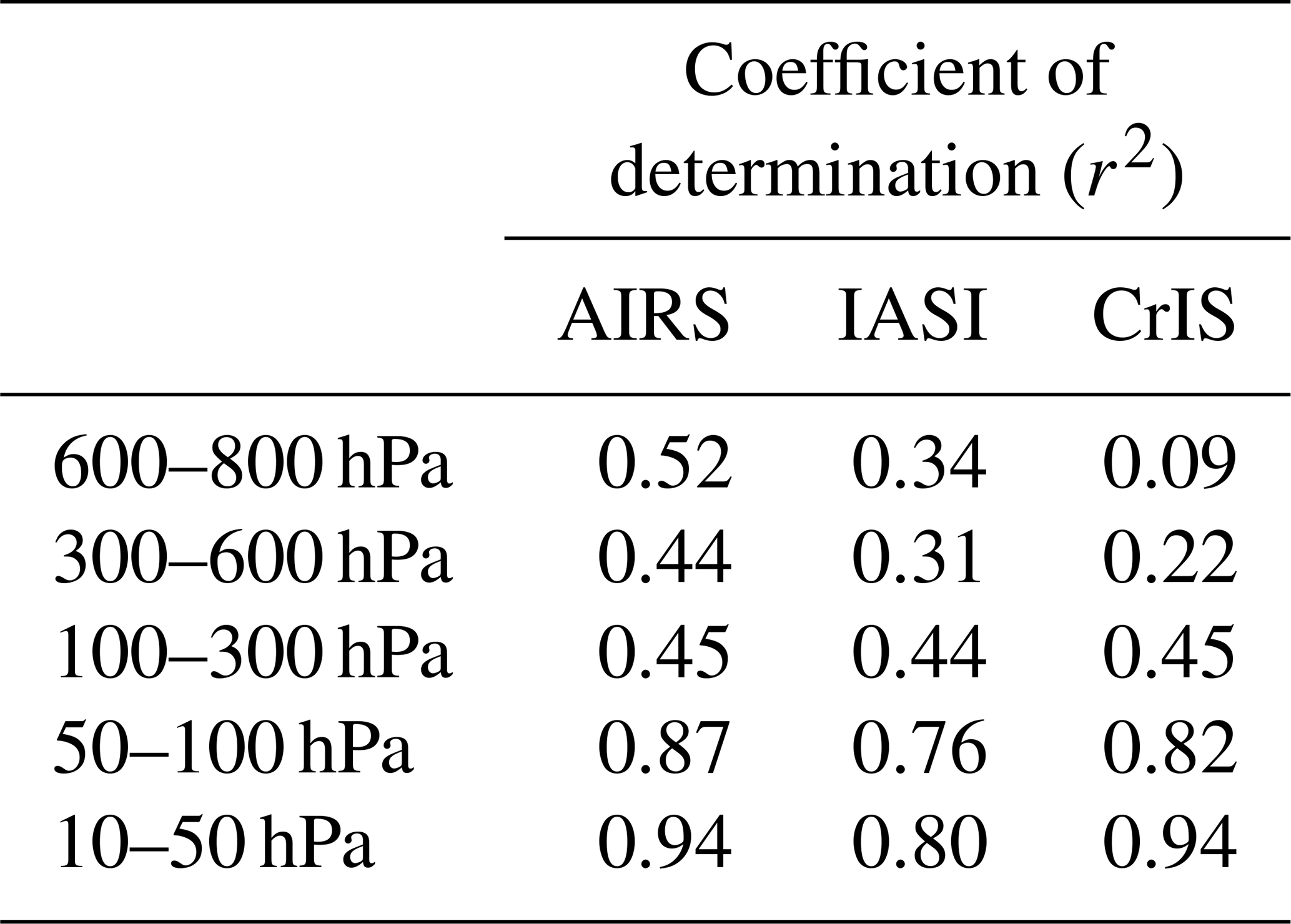
Additionally, Pearson correlations between ozonesondes and IASI, CrIS, and AIRS are also studied at five atmospheric layers (i.e. 600–800, 300–600, 100–300, 50–100, and 10–50 hPa) (Table 2). A relatively stronger positive correlation is found in the middle stratosphere (50–100 hPa) and lower stratosphere (50–100 hPa), which was highest for AIRS, followed by CrIS and IASI, and a relatively low correlation is observed in the middle troposphere (300–600 hPa) for AIRS and IASI (∼ 44 % and 31 %), while CrIS shows the poorest correlation in the lower troposphere of about 9 %. The lower concurrence between ozonesondes and the satellite sensors in the lower troposphere could be due to lower sensitivity and shorter lifetime of near-surface ozone that could increase the a priori contribution and sampling mismatch, respectively.
Table 2Coefficient of determination (r2) of ozone retrievals by three IR satellite sensors (AIRS, IASI, and CrIS) in five broad layers with respect to ozonesonde observations.
3.5 Columnar ozone
3.5.1 Total column ozone (TCO)
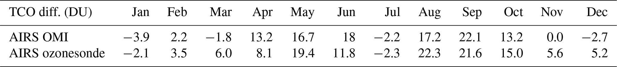
Figure 9a shows variations in monthly average TCO from ozonesondes, AIRS, and OMI during 2011–2017. Here the box plots are also overlaid on the mean column to describe the distribution of monthly column data. In general, the TCO is higher during spring, which subsequently drops in the summer monsoon. AIRS TCO shows a bimodal monthly variation which is not seen in the ozonesonde and OMI observations; otherwise, its monthly variation is in reasonable agreement with the ozonesondes. The OMI TCO has a good match with the ozonesondes with a maximum difference of up to about 5 DU (Dobson units). Table 3 shows the difference in the TCO between AIRS, OMI, and ozonesondes. AIRS shows considerable overestimation in the range of 2.2–22 DU for some months but notable underestimation (1.8–4 DU) for others with respect to both ozonesondes and OMI. The correlation between AIRS TCO and ozonesonde TCO is found to be 0.5 (Table S4). To further understand the cause of bimodal variations in AIRS (higher ozone during August, September, and October), the AIRS ozone profiles were integrated between different stratospheric regions (100–70, 70–50, 50–20, and 20–1 hPa), and we found that the elevated total ozone during the post-monsoon is mainly contributed from the altitude above 50 hPa.
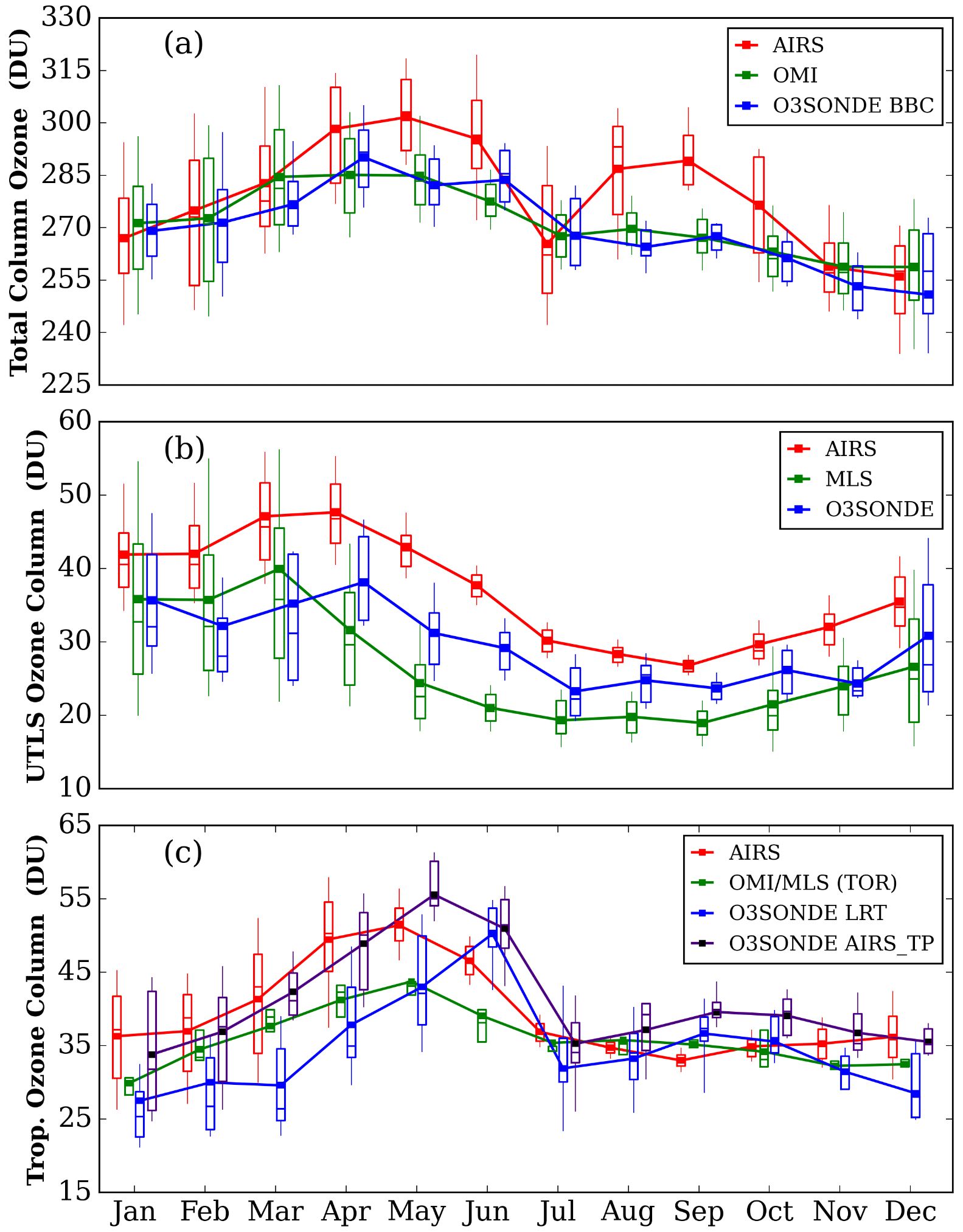
Figure 9(a) Monthly average variations in total column ozone (TCO) for AIRS, OMI, and ozonesonde (balloon-burst climatology) over the central Himalayas for the 2011–2017 period. (b) Monthly average variation in UTLS ozone column for AIRS, MLS, and ozonesondes over the central Himalayas for the 2011–2017 period. (c) Monthly average variations in tropospheric ozone column of AIRS, OMI and MLS (tropospheric ozone residual), and ozonesondes (LRT – sonde lapse rate tropopause) over the central Himalayas for the 2011–2017 period. The ozonesonde tropospheric ozone column is also shown using AIRS tropopause (AIRS_TP). In the box plot, the lower and upper edges of the boxes represent the 25th and 75th percentiles. The whiskers below and above are 10th and 90th percentiles.
Table 3Total column ozone (TCO) differences (in DU) between AIRS, OMI, and ozonesonde during 12 months.
3.5.2 UTLS ozone column
Figure 9b shows the variations in the monthly average UTLS ozone column for collocated and concurrent observations of AIRS, MLS, and ozonesonde during 2011–2017. The UTLS region extends between 400 and 70 hPa (Bian et al., 2007) for ozonesonde and AIRS, while for MLS, the region between 261 and 70 hPa is utilized. The recommended pressure levels for MLS v4 ozone retrieval are above 261 hPa (Livesey et al., 2013; Schwartz et al., 2015). In contrast to TCO, higher ozone in UTLS is seen during the winter and spring (∼ 45 DU) when there are recurring downward transport events, while a clear drop of the column during the summer monsoon shows the convective transport of cleaner oceanic air to the higher altitudes. All the collocated observations are able to capture the monthly variation effectively. However, there is a substantial overestimation by more than 3 DU (Table S5) for all the months in AIRS measurements, and MLS mostly underestimates it except during winter due to smaller integrated columns. Furthermore, the larger whiskers of the box plot during winter and spring show the larger variations in the ozone in the UTLS region. Though there were notable overestimations compared to ozonesondes, UTLS monthly variations are still captured well by AIRS with a correlation of up to 75 % (Table S4). In addition, the correlation of ozonesonde and AIRS ozone at each pressure level in the UTLS region is 0.81, which further increases with ozonesonde (AK) (of about 0.94). The persistent biases in the satellite retrievals arise due to inadequate input parameters that can be improved by using more accurate initial parameters and surface emissivity (Dufour et al., 2012; Boynard et al., 2018).
3.5.3 Tropospheric ozone column
Figure 9c shows the variations in the monthly average tropospheric ozone column utilizing various collocated datasets during 2011–2017. The tropospheric ozone column is calculated by integrating ozone profiles from the surface to the tropopause. The World Meteorological Organization (WMO)-defined lapse rate calculation method is used to calculate tropopause height from balloon-borne and AIRS observations (Fig. 3). Higher tropospheric ozone is observed during the spring and early summer (> 45 DU) when annual crop residue burning events (Fig. S8) occur over northern India, apart from downward transport from the stratosphere. A few cases of downward transport are discussed in the next section. The tropospheric ozone column drops rapidly during the summer monsoon when pristine marine air reaches Nainital. A slight increase in the column is also seen during the autumn, which is again influenced by post-monsoon crop residue burning practices (Fig. S8) over northern India (Bhardwaj et al., 2016). AIRS is able to capture the monthly variations very effectively; however, there are larger biases. The biases with ozonesondes are higher when the tropopause is taken from the balloon-borne observations, while with the AIRS-provided tropopause, the biases are lower than or mostly within the 1σ limit. The correlation between ozonesonde and AIRS, when the AIRS tropopause is used, is very strong (0.72). Like AIRS, the OMI and MLS column is in good agreement and able to produce monthly variations; however, there are larger differences during winter and spring of more than 10 DU. The tropospheric ozone column from ozonesonde is different for balloon-borne LRT and AIRS tropopause, which could be due to the lower vertical resolution of AIRS. AIRS calculates tropopause with an uncertainty of 1–2 km (Divakarla et al., 2006). It can also be seen that on average a lower (about 28 %) tropopause pressure (or higher altitude) is calculated by AIRS compared to ozonesonde measurements (Fig. 3).
3.6 Case studies of biomass burning and downward transport
Over northern India, extensive agriculture practices and forest fires influence ozone at the surface and higher altitudes (Kumar et al., 2011; Cristofanelli et al., 2014; Bhardwaj et al., 2016, 2018). Based on MODIS fire counts, the days in between 1 March and 15 April over northern India are classified as the low fire periods (LFPs) as considered in previous studies over this region. The high fire period (HFP) is classified when the fire counts over the observational site are more than the median fire counts in the biomass burning period, typically from mid-April to May (Bhardwaj et al., 2016). A total of 32 soundings (mid-April to May) are classified as HFPs, and 33 soundings (March to mid-April) are classified as LFPs. Figure 10a shows the average ozone profiles up to 6 km from ozonesonde and AIRS observations during HFPs and LFPs. The ozonesonde data show enhancement in ozone of about 5 to about 11 ppbv during HFPs compared to LFPs, which accounts for a 5 %–20 % increase. It is important to mention that enhancement is greater in higher-altitude regions that drop gradually above 400 hPa. The enhancement is slightly lower (10 %–15 %) in the AIRS profile, where most of it is contributed by the a priori profile (Fig. S11).
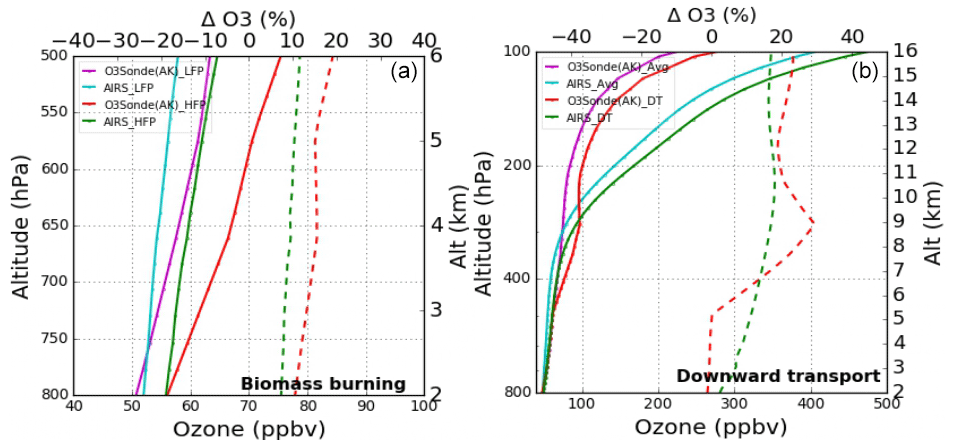
Figure 10(a) Vertical ozone profiles of AIRS ozone and ozonesonde (AK) during low fire period (LFP) and high fire period (HFP). The solid lines correspond to ozone profiles, while the dotted lines show a percentage increase in ozonesonde (red) and AIRS (green) profiles during biomass burning events. (b) Vertical ozone profiles of AIRS ozone and ozonesonde (AK) during events of downward transport. The dotted line shows ozone enhancement during downward transport events.
Deep stratospheric intrusion or the downward transport (DT) of ozone-rich air from the stratosphere to the troposphere significantly influences ozone profiles over the subtropical regions (Zhu et al., 2006; Lal et al., 2014). Over the subtropical Himalayas, such ozone intrusions are observed during the winter and spring seasons (Zhu et al., 2006; Ojha et al., 2014). The DT events are classified based on the higher ozone in the middle–upper troposphere seen from ozonesondes with relatively larger Ertel potential vorticity (EPV) and lower humidity in MERRA-2 reanalysis data. Based on this, 10 soundings (between January and mid-April) are classified as DT events for ozonesondes and AIRS. Figure 10b shows ozone profiles from ozonesonde (AK) and AIRS observations for high-ozone DT events, as well as the average ozone profiles of corresponding months excluding the DT event. Though there are persistent positive biases in the AIRS ozone profile compared to ozonesondes in the middle–upper troposphere, still both the observations have captured the influence of the downward transport on the ozone profile very effectively and show an increase in the ozone of 10 %–20 % in the altitude range of 2–16 km. Ozonesonde-based observations have shown about a 2-fold increase in upper–middle tropospheric ozone due to downward ozone transport over this region (Ojha et al., 2014). Further, the first-guess profile's contribution to AIRS retrieval during DTs is negligible (Fig. S11) and shows the main contribution from the AIRS observations itself. So, despite the persistent biases in the AIRS and ozonesonde observations, AIRS is able to capture the influence of downward transport (DT) on the ozone profile notably well.
3.7 Ozone radiative forcing
Radiative forcing is a valuable metric to estimate the radiative impacts of any anthropogenic or natural activity on the climate system (Ramaswamy, 2001). It measures the net radiation at the surface, tropopause, and the top of the atmosphere due to any atmospheric constituents. Here we discuss the ozone radiative forcing (RF) at the surface in the ultraviolet (UV) spectral range (Antón et al., 2014; Mateos and Antón, 2020) using the ozonesonde, OMI, and AIRS TCO data. The RF is calculated based on Antón et al. (2014), relative to 1979 utilizing total ozone mapping spectrometer (TOMS) TCO data in 1979; monthly averaged solar zenith angles of site; clearness index (Chakraborty et al., 2014, and references therein); and respective monthly average TCO data of AIRS, OMI, and ozonesondes. Rather than quantifying the RF values here, our primary focus is to show how the discrepancies of satellite ozone data (mainly AIRS) can impact the calculation of RF values. Figure 11 shows the seasonal average ozone RF relative to 1979. The annual average ozone RF during 2011–2017 is 4.86, 4.04, and 2.96 mW m−2 for ozonesonde, OMI, and AIRS, respectively. The RF values for ozonesonde and OMI are comparable to Mateos and Antón (2020) (4 mW m−2) for the extratropical region. However, for AIRS, the RF value is lower by 45 %. Further, the seasonal average ozone RF (2011–2017) is consistent between ozonesonde and OMI, while notable differences are seen in AIRS except during the winter season when differences are marginal (Fig. 11). Also, it is noted (Table 3) that the higher total ozone bias during autumn (as high as 22 DU) contributes to higher RF differences in autumn (Fig. 11).
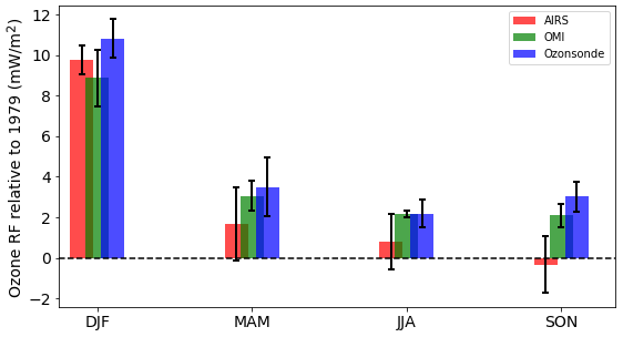
Figure 11Seasonal average ozone UV radiative forcing (RF) relative to 1979 as calculated from ozonesonde, OMI, and AIRS total ozone data for the 2011–2017 period. Spreads correspond to 1 standard deviation.
This study has utilized 242 ECC (EN-SCI) ozone soundings (during 2011–2017) conducted over a Himalayan station (Nainital) to evaluate the AIRS version 6 ozone product and study the performance during biomass burning events, ozone downward transport events, and estimation of ozone radiative forcing. AIRS ozone retrieval is evaluated in terms of retrieval sensitivity, retrieval biases, retrieval errors, and ability to retrieve the natural variability in columnar ozone at different altitude regions. This study is the first of its kind in the Himalayan region and fills the void of proper validation of various satellite ozone retrievals, particularly AIRS, over this complex terrain. The AIRS averaging kernel information is applied to ozonesondes for a like-for-like comparison to overcome their sensitivity differences. The monthly profile evaluation shows ozone peak and ozone altitude dependency is captured well by AIRS retrieval with smaller but notable underestimation (5 %–20 %) in the lower–middle troposphere and stratosphere, while overestimation in the UTLS region is as high as 102 %. We show a relatively higher sensitivity of AIRS ozone for the summer monsoon in the UTLS region, where the biases between AIRS and ozonesonde reduced from 92 % to 19 % after applying AIRS averaging kernel information.
Furthermore, the weighted statistical error analysis of AIRS-retrieved ozone profiles with ozonesonde shows higher positive biases (65 %) and SD (25 %) in the upper troposphere, where a high-resolution satellite MLS agrees well with ozonesonde, while in the lower–middle troposphere and stratosphere, AIRS ozone was negatively biased by less than 20 %. In addition, though the biases and errors are higher in the upper troposphere, there is a larger correlation of about 81 %, demonstrating the reasonable capability of AIRS to retrieve upper-tropospheric ozone variability with certain positive biases. Such biases in satellite retrieval can be eliminated by choosing better emissivity inputs or other retrieval parameters. The histogram of differences between AIRS and ozonesonde (AK) mostly shows an underestimation of AIRS ozone (2.4–39.8 ppbv) except in the upper troposphere, where a notable overestimation with a mean bias of about 43 ppbv is observed. The AIRS ozone retrieval algorithm was further evaluated using the radiance of IASI and CrIS sensors; these sensors provided similar error statistics as seen for AIRS, with higher positive biases in the UTLS region.
The AIRS-derived columnar ozone amounts (i.e. total, UTLS, and tropospheric ozone) are also evaluated to see whether the ozone variability at different altitude regions is being retrieved correctly. The UTLS and tropospheric ozone monthly variations are captured well by AIRS with persistent positive biases. However, the total column ozone shows bimodal monthly variations which were not evident in the ozonesonde and OMI total ozone observations. Further, we found a higher total column ozone in AIRS during autumn, which is mostly coming from the stratospheric region above 50 hPa. Furthermore, the capabilities of AIRS ozone retrieval to capture various biomass burning and downward transport events have also been studied using fire counts and EPV tracers. AIRS captures reasonable enhancements in ozone profiles (5 %–20 %) after such events with notable contributions of the a priori profiles, particularly in biomass burning events.
Unlike the well-mixed greenhouse gases, the ozone RF remains uncertain due to inadequate budget estimates and complex chemical processes. Stevenson et al. (2013) have shown that uncertainties in ozone concentrations of a few percent can produce a spread of ∼ 17 % in ozone RF estimations. The total ozone discrepancies of AIRS lead to lower RF (by about 45 %) compared to ozonesonde and OMI and higher uncertainty in this Himalayan region. Here, the role of in situ observations from ozone soundings is shown to be important in improving the satellite-retrieved ozone over the Himalayan region by assessing and providing insights into its errors and biases. This information over the Himalayan region could be applied to the ozone retrieval from other satellite datasets, having long-term coverage. Such an evaluation study is crucial for reducing biases in satellite retrievals and assessing the credibility of various space-based ozone retrievals over the Himalayan region. It will also help us better understand regional ozone and radiation budgets over this Himalayan region and perceive the possible differences between satellites and truth observations.
AIRS, MLS, and OMI data are available from the open archive of NASA Goddard Space Flight Center Earth Sciences Data and Information Services Center (NASA GES DISC). The data are accessed from the AIRS (https://doi.org/10.5067/Aqua/AIRS/DATA208, AIRS Science Team and Teixeira, 2013, NASA GES DISC), MLS (https://doi.org/10.5067/Aura/MLS/DATA2017, Schwartz, et al., 2015, NASA GES DISC), and OMI (https://doi.org/10.5067/Aura/OMI/DATA2025, Bhartia, 2012, NASA GES DISC) websites. IASI and CrIS data based on NUCAPS retrieval can be accessed through the NOAA CLASS portal (https://www.avl.class.noaa.gov, Susskind, et al., 2003, NOAA CLASS). OMI and MLS tropospheric ozone column data can be obtained from (https://acd-ext.gsfc.nasa.gov/Data_services/cloud_slice/new_data.html, Ziemke et al., 2006, NASA GSFC). Ozonesonde data can be made available upon a reasonable request in writing to the corresponding author.
The supplement related to this article is available online at: https://doi.org/10.5194/amt-16-889-2023-supplement.
PR and MN designed the study and operated the ozonesonde, performed the data analysis, interpreted the results, and wrote the initial draft of the paper. PKT and RK helped to understand the different satellite retrievals and their respective sensitivity. EF helped to understand the averaging kernel matrix of the satellite retrieval. SL, SNT, PB, AJ, and SV provided significant conceptual input to the design of the manuscript and the improvement of the revised manuscript. All authors discussed the results and commented on the paper in various stages.
The contact author has declared that none of the authors has any competing interests.
Publisher’s note: Copernicus Publications remains neutral with regard to jurisdictional claims in published maps and institutional affiliations.
This article is part of the special issue “Atmospheric ozone and related species in the early 2020s: latest results and trends (ACP/AMT inter-journal SI)”. It is a result of the 2021 Quadrennial Ozone Symposium (QOS) held online on 3–9 October 2021.
We are grateful to the director of ARIES and the ISRO ATCTM project for supporting this work. Help from Deeapak Chausali and Nitin Pal in balloon launches and coordination with the air traffic control is highly acknowledged. The National Center for Atmospheric Research is sponsored by the National Science Foundation. Shyam Lal is grateful to INSA, New Delhi, for the position and the director of PRL, Ahmedabad, for the support. We highly acknowledge NOAA and NASA-EARTHDATA online data portals for providing IASI, AIRS, and CrIS level 2 data. We thank the NASA Goddard Space Flight Center Ozone Processing Team for providing the OMI and MLS tropospheric ozone and OMI total column ozone, as well as the Jet Propulsion Laboratory (JPL) for the MLS ozone profile. We would also like to acknowledge the use of the MODIS fire data through FIRMS archive download. The use of maps from Google Earth is also acknowledged. We thank the reviewers for their constructive comments and valuable suggestions.
This research has been supported by the Indian Space Research Organisation (project ATCTM) and ARIES.
This paper was edited by Ja-Ho Koo and reviewed by Pawan K. Bhartia and two anonymous referees.
Aghedo, A. M., Bowman, K. W., Worden, H. M., Kulawik, S. S., Shindell, D. T., Lamarque, J. F., Faluvegi, G., Parrington, M., Jones, D. B. A., and Rast, S.: The vertical distribution of ozone instantaneous radiative forcing from satellite and chemistry climate models, J. Geophys. Res.-Atmos., 116, D01305, https://doi.org/10.1029/2010JD014243, 2011.
AIRS Science Team and Teixeira, J.: AIRS/Aqua L2 Support Retrieval (AIRS-only) V006, Greenbelt, MD, USA, Goddard Earth Sciences Data and Information Services Center (GES DISC) [data set], https://doi.org/10.5067/Aqua/AIRS/DATA208, 2013.
Antón, M., Mateos, D., Román, R., Valenzuela, A., Alados-Arboledas, L., and Olmo, F. J.: A method to determine the ozone radiative forcing in the ultra-violet range from experimental data, J. Geophys. Res.-Atmos., 119, 1860–1873, https://doi.org/10.1002/2013JD020444, 2014.
Bai, W., Wu, C., Li, J., and Wang, W.: Impact of terrain altitude and cloud height on ozone remote sensing from satellite, J. Atmos. Ocean. Tech., 31, 903–912, 2014.
Barré, J., Peuch, V.-H., Attié, J.-L., El Amraoui, L., Lahoz, W. A., Josse, B., Claeyman, M., and Nédélec, P.: Stratosphere-troposphere ozone exchange from high resolution MLS ozone analyses, Atmos. Chem. Phys., 12, 6129–6144, https://doi.org/10.5194/acp-12-6129-2012, 2012.
Bhardwaj, P., Naja, M., Kumar, R., and Chandola, H. C.: Seasonal, interannual, and long-term variabilities in biomass burning activity over South Asia, Environ. Sci. Pollut. R., 23, 4397–4410, 2016.
Bhardwaj, P., Naja, M., Rupakheti, M., Lupascu, A., Mues, A., Panday, A. K., Kumar, R., Mahata, K. S., Lal, S., Chandola, H. C., and Lawrence, M. G.: Variations in surface ozone and carbon monoxide in the Kathmandu Valley and surrounding broader regions during SusKat-ABC field campaign: role of local and regional sources, Atmos. Chem. Phys., 18, 11949–11971, https://doi.org/10.5194/acp-18-11949-2018, 2018.
Bhartia, P. K.: OMI/Aura Ozone (O3) Total Column Daily L2 Global Gridded 0.25 degree × 0.25 degree V3, Goddard Earth Sciences Data and Information Services Center (GES DISC) [data set], https://doi.org/10.5067/Aura/OMI/DATA2025, 2012.
Bhartia, P. K., McPeters, R. D., Mateer, C. L., Flynn, L. E., and Wellemeyer, C.: Algorithm for the estimation of vertical ozone profiles from the backscattered ultraviolet technique, J. Geophys. Res.-Atmos., 101, 18793–18806, 1996.
Bian, J., Gettelman, A., Chen, H., and Pan, L. L.: Validation of satellite ozone profile retrievals using Beijing ozonesonde data, J. Geophys. Res.-Atmos., 112, D06305, https://doi.org/10.1029/2006JD007502, 2007.
Boynard, A., Hurtmans, D., Koukouli, M. E., Goutail, F., Bureau, J., Safieddine, S., Lerot, C., Hadji-Lazaro, J., Wespes, C., Pommereau, J.-P., Pazmino, A., Zyrichidou, I., Balis, D., Barbe, A., Mikhailenko, S. N., Loyola, D., Valks, P., Van Roozendael, M., Coheur, P.-F., and Clerbaux, C.: Seven years of IASI ozone retrievals from FORLI: validation with independent total column and vertical profile measurements, Atmos. Meas. Tech., 9, 4327–4353, https://doi.org/10.5194/amt-9-4327-2016, 2016.
Boynard, A., Hurtmans, D., Garane, K., Goutail, F., Hadji-Lazaro, J., Koukouli, M. E., Wespes, C., Vigouroux, C., Keppens, A., Pommereau, J.-P., Pazmino, A., Balis, D., Loyola, D., Valks, P., Sussmann, R., Smale, D., Coheur, P.-F., and Clerbaux, C.: Validation of the IASI FORLI/EUMETSAT ozone products using satellite (GOME-2), ground-based (Brewer–Dobson, SAOZ, FTIR) and ozonesonde measurements, Atmos. Meas. Tech., 11, 5125–5152, https://doi.org/10.5194/amt-11-5125-2018, 2018.
Brunamonti, S., Jorge, T., Oelsner, P., Hanumanthu, S., Singh, B. B., Kumar, K. R., Sonbawne, S., Meier, S., Singh, D., Wienhold, F. G., Luo, B. P., Boettcher, M., Poltera, Y., Jauhiainen, H., Kayastha, R., Karmacharya, J., Dirksen, R., Naja, M., Rex, M., Fadnavis, S., and Peter, T.: Balloon-borne measurements of temperature, water vapor, ozone and aerosol backscatter on the southern slopes of the Himalayas during StratoClim 2016–2017, Atmos. Chem. Phys., 18, 15937–15957, https://doi.org/10.5194/acp-18-15937-2018, 2018.
Cazorla, M., and Herrera, E.: An ozonesonde evaluation of spaceborne observations in the Andean tropics, Sci. Rep., 12, 1–8, 2022.
Chakraborty, S., Sadhu, P. K., and Nitai, P. A. L.: New location selection criterions for solar PV power plant, International Journal of Renewable Energy Research, 4, 1020–1030, 2014.
Clerbaux, C., Hadji-Lazaro, J., Turquety, S., George, M., Coheur, P. F., Hurtmans, D., Wespes, C., Herbin, H., Blumstein, D., Tourniers, B., and Phulpin, T.: The IASI/MetOp1 Mission: First observations and highlights of its potential contribution to GMES2, Space Research Today, 168, 19–24, 2007.
Coheur, P. F., Barret, B., Turquety, S., Hurtmans, D., Hadji-Lazaro, J., and Clerbaux, C.: Retrieval and characterization of ozone vertical profiles from a thermal infrared nadir sounder, J. Geophys. Res.-Atmos., 110, D24303, https://doi.org/10.1029/2005JD005845, 2005.
Cristofanelli, P., Putero, D., Adhikary, B., Landi, T. C., Marinoni, A., Duchi, R., Calzolari, F., Laj, P., Stocchi, P., Verza, G., and Vuillermoz, E.: Transport of short-lived climate forcers/pollutants (SLCF/P) to the Himalayas during the South Asian summer monsoon onset, Environ. Res. Lett., 9, 084005, https://doi.org/10.1088/1748-9326/9/8/084005, 2014.
Divakarla, M., Barnet, C., Goldberg, M., Maddy, E., Wolf, W., Flynn, L., Xiong, X., Wei, J., Zhou, L., and Liu, X.: Validation of Atmospheric Infrared Sounder (AIRS) temperature, water vapor, and ozone retrievals with matched radiosonde and ozonesonde measurements and forecasts, Proc. SPIE 6405, Multispectral, Hyperspectral, and Ultraspectral Remote Sensing Technology, Techniques, and Applications, 640503, https://doi.org/10.1117/12.694116, 2006.
Divakarla, M., Barnet, C., Goldberg, M., Maddy, E., Irion, F., Newchurch, M., Liu, X., Wolf, W., Flynn, L., Labow, G., and Xiong, X.: Evaluation of Atmospheric Infrared Sounder ozone profiles and total ozone retrievals with matched ozonesonde measurements, ECMWF ozone data, and Ozone Monitoring Instrument retrievals, J. Geophys. Res.-Atmos., 113, D15308, https://doi.org/10.1029/2007JD009317, 2008.
Dufour, G., Eremenko, M., Griesfeller, A., Barret, B., LeFlochmoën, E., Clerbaux, C., Hadji-Lazaro, J., Coheur, P.-F., and Hurtmans, D.: Validation of three different scientific ozone products retrieved from IASI spectra using ozonesondes, Atmos. Meas. Tech., 5, 611–630, https://doi.org/10.5194/amt-5-611-2012, 2012.
Ebi, K. L. and McGregor, G.: Climate change, tropospheric ozone and particulate matter, and health impacts, Environ. Health Persp., 116, 1449–1455, 2008.
Fadnavis, S., Dhomse, S., Ghude, S., Iyer, U., Buchunde, P., Sonbawne, S., and Raj, P. E.: Ozone trends in the vertical structure of Upper Troposphere and Lower stratosphere over the Indian monsoon region, Int. J. Environ. Sci. Te., 11, 529–542, 2014.
Fishbein, E., Farmer, C. B., Granger, S. L., Gregorich, D. T., Gunson, M. R., Hannon, S. E., Hofstadter, M. D., Lee, S. Y., Leroy, S. S., and Strow, L. L.: Formulation and validation of simulated data for the Atmospheric Infrared Sounder (AIRS), IEEE T. Geosci. Remote, 41, 314–329, 2003.
Fishman, J. and Larsen, J. C.: Distribution of total ozone and stratospheric ozone in the tropics: Implications for the distribution of tropospheric ozone, J. Geophys. Res.-Atmos., 92, 6627–6634, 1987.
Fishman, J., Ramanathan, V., Crutzen, P. J., and Liu, S. C.: Tropospheric ozone and climate, Nature, 282, 818–820, 1979.
Foret, G., Eremenko, M., Cuesta, J., Sellitto, P., Barré, J., Gaubert, B., Coman, A., Dufour, G., Liu, X., Joly, M., and Doche, C.: Ozone pollution: What can we see from space? A case study, J. Geophys. Res.-Atmos., 119, 8476–8499, 2014.
Forster, P. M., Bodeker, G., Schofield, R., Solomon, S., and Thompson, D.: Effects of ozone cooling in the tropical lower stratosphere and upper troposphere, Geophys. Res. Lett., 34, L23813, https://doi.org/10.1029/2007GL031994, 2007.
Gauss, M., Myhre, G., Pitari, G., Prather, M. J., Isaksen, I. S. A., Berntsen, T. K., Brasseur, G. P., Dentener, F. J., Derwent, R. G., Hauglustaine, D. A., and Horowitz, L. W.: Radiative forcing in the 21st century due to ozone changes in the troposphere and the lower stratosphere, J. Geophys. Res.-Atmos., 108, 4292, https://doi.org/10.1029/2002JD002624, 2003.
Hauglustaine, D. A. and Brasseur, G. P.: Evolution of tropospheric ozone under anthropogenic activities and associated radiative forcing of climate, J. Geophys. Res.-Atmos., 106, 32337–32360, 2001.
Hegglin, M. I., Fahey, D. W., McFarland, M., Montzka, S. A., and Nash, E. R.: Twenty questions and answers about the ozone layer: 2014 update, Scientific Assessment of Ozone Depletion: 2014, World Meteorological Organization, Geneva, Switzerland, 84 pp., ISBN 978-9966-076-02-1, 2015.
Hudson, R. D. and Thompson, A. M.: Tropical tropospheric ozone from total ozone mapping spectrometer by a modified residual method, J. Geophys. Res.-Atmos., 103, 22129–22145, 1998.
Irion, F. W., Kahn, B. H., Schreier, M. M., Fetzer, E. J., Fishbein, E., Fu, D., Kalmus, P., Wilson, R. C., Wong, S., and Yue, Q.: Single-footprint retrievals of temperature, water vapor and cloud properties from AIRS, Atmos. Meas. Tech., 11, 971–995, https://doi.org/10.5194/amt-11-971-2018, 2018.
Kim, J. H. and Newchurch, M. J.: Climatology and trends of tropospheric ozone over the eastern Pacific Ocean: The influences of biomass burning and tropospheric dynamics, Geophys. Res. Lett., 23, 3723–3726, 1996.
Komhyr, W. D.: Nonreactive gas sampling pump, Rev. Sci. Instrum., 38, 981–983, 1967.
Komhyr, W. D., Barnes, R. A., Brothers, G. B., Lathrop, J. A., and Opperman, D. P.: Electrochemical concentration cell ozonesonde performance evaluation during STOIC 1989, J. Geophys. Res.-Atmos., 100, 9231–9244, 1995.
Kumar, R., Naja, M., Satheesh, S. K., Ojha, N., Joshi, H., Sarangi, T., Pant, P., Dumka, U. C., Hegde, P., and Venkataramani, S.: Influences of the springtime northern Indian biomass burning over the central Himalayas, J. Geophys. Res.-Atmos., 116, D19302, https://doi.org/10.1029/2010JD015509, 2011.
Kumar, R., Naja, M., Pfister, G. G., Barth, M. C., and Brasseur, G. P.: Simulations over South Asia using the Weather Research and Forecasting model with Chemistry (WRF-Chem): set-up and meteorological evaluation, Geosci. Model Dev., 5, 321–343, https://doi.org/10.5194/gmd-5-321-2012, 2012a.
Kumar, R., Naja, M., Pfister, G. G., Barth, M. C., Wiedinmyer, C., and Brasseur, G. P.: Simulations over South Asia using the Weather Research and Forecasting model with Chemistry (WRF-Chem): chemistry evaluation and initial results, Geosci. Model Dev., 5, 619–648, https://doi.org/10.5194/gmd-5-619-2012, 2012b.
Lacis, A. A., Wuebbles, D. J., and Logan, J. A.: Radiative forcing of climate by changes in the vertical distribution of ozone, J. Geophys. Res.-Atmos., 95, 9971–9981, 1990.
Lal, S., Venkataramani, S., Srivastava, S., Gupta, S., Naja, M., Sarangi, T., and Liu, X.: Transport effects on the vertical distribution of tropospheric ozone over the tropical marine regions surrounding India, J. Geophys. Res., 118, 1513–1524, https://doi.org/10.1002/jgrd.50180, 2013.
Lal, S., Venkataramani, S., Chandra, N., Cooper, O. R., Brioude, J., and Naja, M.: Transport effects on the vertical distribution of tropospheric ozone over western India, J. Geophys. Res.-Atmos., 119, 10012–10026, https://doi.org/10.1002/2014JD021854, 2014.
Lal, S., Venkataramani, S., Naja, M., Kuniyal, J. C., Mandal, T. K., Bhuyan, P. K., Kumari, K. M., Tripathi, S. N., Sarkar, U., Das, T., and Swamy, Y. V.: Loss of crop yields in India due to surface ozone: An estimation based on a network of observations, Environ. Sci. Pollut. R., 24, 20972–20981, 2017.
Lawrence, M. G. and Lelieveld, J.: Atmospheric pollutant outflow from southern Asia: a review, Atmos. Chem. Phys., 10, 11017–11096, https://doi.org/10.5194/acp-10-11017-2010, 2010.
Lelieveld, J., Haines, A., and Pozzer, A.: Age-dependent health risk from ambient air pollution: a modelling and data analysis of childhood mortality in middle-income and low-income countries, Lancet Planetary Health, 2, e292–e300, 2018.
Livesey, N. J., Logan, J. A., Santee, M. L., Waters, J. W., Doherty, R. M., Read, W. G., Froidevaux, L., and Jiang, J. H.: Interrelated variations of O3, CO and deep convection in the tropical/subtropical upper troposphere observed by the Aura Microwave Limb Sounder (MLS) during 2004–2011, Atmos. Chem. Phys., 13, 579–598, https://doi.org/10.5194/acp-13-579-2013, 2013.
Lu, X., Zhang, L., Liu, X., Gao, M., Zhao, Y., and Shao, J.: Lower tropospheric ozone over India and its linkage to the South Asian monsoon, Atmos. Chem. Phys., 18, 3101–3118, https://doi.org/10.5194/acp-18-3101-2018, 2018.
Maddy, E. S. and Barnet, C. D.: Vertical resolution estimates in version 5 of AIRS operational retrievals, IEEE T. Geosci. Remote, 46, 2375–2384, 2008.
Mateos, D. and Antón, M.: Worldwide Evaluation of Ozone Radiative Forcing in the UV-B Range between 1979 and 2014, Remote Sens., 12, 436, https://doi.org/10.3390/rs12030436, 2020.
McPeters, R. D. and Labow, G. J.: Climatology 2011: An MLS and sonde derived ozone climatology for satellite retrieval algorithms, J. Geophys. Res.-Atmos., 117, D10303, https://doi.org/10.1029/2011JD017006, 2012.
McPeters, R. D., Labow, G. J., and Logan, J. A.: Ozone climatological profiles for satellite retrieval algorithms, J. Geophys. Res.-Atmos., 112, D05308, https://doi.org/10.1029/2005JD006823, 2007.
Monahan, K. P., Pan, L. L., McDonald, A. J., Bodeker, G. E., Wei, J., George, S. E., Barnet, C. D., and Maddy, E.: Validation of AIRS v4 ozone profiles in the UTLS using ozonesondes from Lauder, NZ and Boulder, USA, J. Geophys. Res.-Atmos., 112, D17304, https://doi.org/10.1029/2006JD008181, 2007.
Monks, P. S., Archibald, A. T., Colette, A., Cooper, O., Coyle, M., Derwent, R., Fowler, D., Granier, C., Law, K. S., Mills, G. E., Stevenson, D. S., Tarasova, O., Thouret, V., von Schneidemesser, E., Sommariva, R., Wild, O., and Williams, M. L.: Tropospheric ozone and its precursors from the urban to the global scale from air quality to short-lived climate forcer, Atmos. Chem. Phys., 15, 8889–8973, https://doi.org/10.5194/acp-15-8889-2015, 2015.
Myhre, G., Aas, W., Cherian, R., Collins, W., Faluvegi, G., Flanner, M., Forster, P., Hodnebrog, Ø., Klimont, Z., Lund, M. T., Mülmenstädt, J., Lund Myhre, C., Olivié, D., Prather, M., Quaas, J., Samset, B. H., Schnell, J. L., Schulz, M., Shindell, D., Skeie, R. B., Takemura, T., and Tsyro, S.: Multi-model simulations of aerosol and ozone radiative forcing due to anthropogenic emission changes during the period 1990–2015, Atmos. Chem. Phys., 17, 2709–2720, https://doi.org/10.5194/acp-17-2709-2017, 2017.
Naja, M., Mallik, C., Sarangi, T., Sheel, V., and Lal, S.: SO2 measurements at a high altitude site in the central Himalayas: Role of regional transport, Atmos. Environ., 99, 392–402, https://doi.org/10.1016/j.atmosenv.2014.08.031, 2014.
Naja, M., Bhardwaj, P., Singh, N., Kumar, P., Kumar, R., Ojha, N., Sagar, R., Satheesh, S. K., Moorthy, K. K., and Kotamarthi, V. R.: High-frequency vertical profiling of meteorological parameters using AMF1 facility during RAWEX–GVAX at ARIES, Nainital, Curr. Sci. India, 111, 132–140, https://doi.org/10.18520/cs/v111/i1/132-140, 2016.
Nalli, N. R., Barnet, C. D., Reale, A., Tobin, D., Gambacorta, A., Maddy, E. S., Joseph, E., Sun, B., Borg, L., Mollner, A. K., and Morris, V. R.: Validation of satellite sounder environmental data records: Application to the Cross-track Infrared Microwave Sounder Suite, J. Geophys. Res.-Atmos., 118, 13–628, 2013.
Nalli, N. R., Gambacorta, A., Liu, Q., Tan, C., Iturbide-Sanchez, F., Barnet, C. D., Joseph, E., Morris, V. R., Oyola, M., and Smith, J. W.: Validation of Atmospheric Profile Retrievals from the SNPP NOAA-Unique Combined Atmospheric Processing System. Part 2: Ozone, IEEE T. Geosci. Remote, 56, 598–607, 2017.
Ojha, N., Naja, M., Sarangi, T., Kumar, R., Bhardwaj, P., Lal, S., Venkataramani, S., Sagar, R., Kumar, A., and Chandola, H. C.: On the processes influencing the vertical distribution of ozone over the central Himalayas: Analysis of yearlong ozonesonde observations, Atmos. Environ., 88, 201–211, 2014.
Pagano, T. S., Aumann, H. H., Hagan, D. E., and Overoye, K.: Prelaunch and in-flight radiometric calibration of the Atmospheric Infrared Sounder (AIRS), IEEE T. Geosci. Remote, 41, 265–273, 2003.
Pierce, R. B., Al-Saadi, J., Kittaka, C., Schaack, T., Lenzen, A., Bowman, K., Szykman, J., Soja, A., Ryerson, T., Thompson, A. M., and Bhartia, P.: Impacts of background ozone production on Houston and Dallas, Texas, air quality during the Second Texas Air Quality Study field mission, J. Geophys. Res.-Atmos., 114, D00F09, https://doi.org/10.1029/2008JD011337, 2009.
Pittman, J. V., Pan, L. L., Wei, J. C., Irion, F. W., Liu, X., Maddy, E. S., Barnet, C. D., Chance, K., and Gao, R. S.: Evaluation of AIRS, IASI, and OMI ozone profile retrievals in the extratropical tropopause region using in situ aircraft measurements, J. Geophys. Res.-Atmos., 114, D24109, https://doi.org/10.1029/2009JD012493, 2009.
Ramaswamy, V.: Radiative forcing of climate change, Climate Change 2001: The Scientific Basis, Contribution of Working Group I to the Third Assessment Report of the Intergovernmental Panel on Climate Change, Cambridge University Press, Cambridge, UK, p. 351, https://www.ipcc.ch/site/assets/uploads/2018/03/WGI_TAR_full_report.pdf (last access: 15 February 2023), 2001.
Rawat, P. and Naja, M.: Remote sensing study of ozone, NO2, and CO: some contrary effects of SARS-CoV-2 lockdown over India, Environ. Sci. Pollut. R., 29, 22515–22530, https://doi.org/10.1007/s11356-021-17441-2, 2021.
Rawat, P., Naja, M., Thapliyal, P. K., Srivastava, S., Bhardwaj, P., Kumar, R., Bhatacharjee, S., Venkatramani, S., Tiwari, S. N., and Lal, S.: Assessment of vertical ozone profiles from INSAT-3D sounder over the Central Himalaya, Curr. Sci. India, 119, 1113, https://doi.org/10.18520/cs/v119/i7/1113-1122, 2020.
Rodgers, C. D.: Retrieval of atmospheric temperature and composition from remote measurements of thermal radiation, Rev. Geophys., 14, 609–624, 1976.
Rodgers, C. D.: Characterization and error analysis of profiles retrieved from remote sounding measurements, J. Geophys. Res.-Atmos., 95, 5587–5595, 1990.
Rodgers, C. D. and Connor, B. J.: Intercomparison of remote sounding instruments, J. Geophys. Res.-Atmos., 108, 4116, https://doi.org/10.1029/2002JD002299, 2003.
Sarangi, T., Naja, M., Ojha, N., Kumar, R., Lal, S., Venkataramani, S., Kumar, A., Saga, R., and Chandola, H. C.: First simultaneous measurements of ozone, CO and NOy at a high altitude regional representative site in the central Himalayas, J. Geophys. Res., 119, 1592–1611, https://doi.org/10.1002/2013JD020631, 2014.
Schwartz, M., Froidevaux, L., Livesey, N., and Read, W.: MLS/Aura Level 2 Ozone (O3) Mixing Ratio V004, Greenbelt, MD, USA, Goddard Earth Sciences Data and Information Services Center (GES DISC), https://doi.org/10.5067/Aura/MLS/DATA2017, 2015.
Shindell, D., Kuylenstierna, J. C., Vignati, E., van Dingenen, R., Amann, M., Klimont, Z., Anenberg, S. C., Muller, N., Janssens-Maenhout, G., Raes, F., and Schwartz, J.: Simultaneously mitigating near-term climate change and improving human health and food security, Science, 335, 183–189, 2012.
Smit, H. G., Straeter, W., Johnson, B. J., Oltmans, S. J., Davies, J., Tarasick, D. W., Hoegger, B., Stubi, R., Schmidlin, F. J., Northam, T., and Thompson, A. M.: Assessment of the performance of ECC-ozonesondes under quasi-flight conditions in the environmental simulation chamber: Insights from the Juelich Ozone Sonde Intercomparison Experiment (JOSIE), J. Geophys. Res.-Atmos., 112, D19306, https://doi.org/10.1029/2006JD007308, 2007.
Smit, H. G. J. and the Panel for the Assessment of Standard Operating Procedures for Ozonesondes (ASOPOS 2.0): Ozonesonde Measurement Principles and Best Operational Practices, World Meteorological Organization, GAW Report, 268, https://library.wmo.int/doc_num.php?explnum_id=10884 (last access: 22 June 2022), 2021.
Srivastava, S., Naja, M., and Thouret, V.: Influences of regional pollution and long range transport over Hyderabad using ozone data from MOZAIC, Atmos. Environ., 117, 135–146, 2015.
Stauffer, R. M., Thompson, A. M., Kollonige, D. E., Tarasick, D. W., Van Malderen, R., Smit, H. G., Vömel, H., Morris, G. A., Johnson, B. J., Cullis, P. D., and Stübi, R.: An examination of the recent stability of ozonesonde global network data, Earth and Space Science, 9, e2022EA002459, https://doi.org/10.1029/2022EA002459, 2022.
Stevenson, D. S., Young, P. J., Naik, V., Lamarque, J.-F., Shindell, D. T., Voulgarakis, A., Skeie, R. B., Dalsoren, S. B., Myhre, G., Berntsen, T. K., Folberth, G. A., Rumbold, S. T., Collins, W. J., MacKenzie, I. A., Doherty, R. M., Zeng, G., van Noije, T. P. C., Strunk, A., Bergmann, D., Cameron-Smith, P., Plummer, D. A., Strode, S. A., Horowitz, L., Lee, Y. H., Szopa, S., Sudo, K., Nagashima, T., Josse, B., Cionni, I., Righi, M., Eyring, V., Conley, A., Bowman, K. W., Wild, O., and Archibald, A.: Tropospheric ozone changes, radiative forcing and attribution to emissions in the Atmospheric Chemistry and Climate Model Intercomparison Project (ACCMIP), Atmos. Chem. Phys., 13, 3063–3085, https://doi.org/10.5194/acp-13-3063-2013, 2013.
Susskind, J., Barnet, C. D., and Blaisdell, J. M.: Retrieval of atmospheric and surface parameters from AIRS/AMSU/HSB data in the presence of clouds, IEEE T. Geosci. Remote, 41, 390–409, 2003 (data available at: https://www.avl.class.noaa.gov, last access: 27 August 2022).
Susskind, J., Barnet, C., Blaisdell, J., Iredell, L., Keita, F., Kouvaris, L., Molnar, G., and Chahine, M.: Accuracy of geophysical parameters derived from Atmospheric Infrared Sounder/Advanced Microwave Sounding Unit as a function of fractional cloud cover, J. Geophys. Res.-Atmos., 111, D09S17, https://doi.org/10.1029/2005JD006272, 2006.
Tarasick, D., Galbally, I. E., Cooper, O. R., Schultz, M. G., Ancellet, G., Leblanc, T., Wallington, T. J., Ziemke, J., Liu, X., Steinbacher, M., and Staehelin, J.: Tropospheric Ozone Assessment Report: Tropospheric ozone from 1877 to 2016, observed levels, trends and uncertainties, Elem. Sci. Anthro., 7, 39, https://doi.org/10.1525/elementa.376, 2019.
Thornhill, G. D., Collins, W. J., Kramer, R. J., Olivié, D., Skeie, R. B., O'Connor, F. M., Abraham, N. L., Checa-Garcia, R., Bauer, S. E., Deushi, M., Emmons, L. K., Forster, P. M., Horowitz, L. W., Johnson, B., Keeble, J., Lamarque, J.-F., Michou, M., Mills, M. J., Mulcahy, J. P., Myhre, G., Nabat, P., Naik, V., Oshima, N., Schulz, M., Smith, C. J., Takemura, T., Tilmes, S., Wu, T., Zeng, G., and Zhang, J.: Effective radiative forcing from emissions of reactive gases and aerosols – a multi-model comparison, Atmos. Chem. Phys., 21, 853–874, https://doi.org/10.5194/acp-21-853-2021, 2021.
Veefkind, J. P., de Haan, J. F., Brinksma, E. J., Kroon, M., and Levelt, P. F.: Total ozone from the Ozone Monitoring Instrument (OMI) using the DOAS technique, IEEE T. Geosci. Remote, 44, 1239–1244, 2006.
Verstraeten, W. W., Boersma, K. F., Zörner, J., Allaart, M. A. F., Bowman, K. W., and Worden, J. R.: Validation of six years of TES tropospheric ozone retrievals with ozonesonde measurements: implications for spatial patterns and temporal stability in the bias, Atmos. Meas. Tech., 6, 1413–1423, https://doi.org/10.5194/amt-6-1413-2013, 2013.
Wang, B., Wu, R., and Lau, K.-M.: Interannual variability of Asian summer monsoon: Contrast between the Indian and western North Pacific-East Asian monsoons, J. Climate, 14, 4073–4090, 2001.
Wang, H. R., Damadeo, R., Flittner, D., Kramarova, N., Taha, G., Davis, S., Thompson, A. M., Strahan, S., Wang, Y., Froidevaux, L., and Degenstein, D.: Validation of SAGE III/ISS Solar Occultation Ozone Products With Correlative Satellite and Ground-Based Measurements, J. Geophys. Res.-Atmos., 125, e2020JD032430, https://doi.org/10.1029/2020JD032430, 2020.
Wang, W., Cheng, T., van der A, R. J., de Laat, J., and Williams, J. E.: Verification of the Atmospheric Infrared Sounder (AIRS) and the Microwave Limb Sounder (MLS) ozone algorithms based on retrieved daytime and night-time ozone, Atmos. Meas. Tech., 14, 1673–1687, https://doi.org/10.5194/amt-14-1673-2021, 2021.
Wang, W. C., Zhuang, Y. C., and Bojkov, R. D.: Climate implications of observed changes in ozone vertical distributions at middle and high latitudes of the Northern Hemisphere, Geophys. Res. Lett., 20, 1567–1570, 1993.
Zhang, L., Jacob, D. J., Liu, X., Logan, J. A., Chance, K., Eldering, A., and Bojkov, B. R.: Intercomparison methods for satellite measurements of atmospheric composition: application to tropospheric ozone from TES and OMI, Atmos. Chem. Phys., 10, 4725–4739, https://doi.org/10.5194/acp-10-4725-2010, 2010.
Zhu, T., Lin, W., Song, Y., Cai, X., Zou, H., Kang, L., Zhou, L., and Akimoto, H.: Downward transport of ozone-rich air near Mt. Everest, Geophys. Res. Lett., 33, L23809, https://doi.org/10.1029/2006GL027726, 2006.
Ziemke, J. R., Chandra, S., and Bhartia, P. K.: Two new methods for deriving tropospheric column ozone from TOMS measurements: Assimilated UARS MLS/HALOE and convective-cloud differential techniques, J. Geophys. Res.-Atmos., 103, 22115–22127, 1998.
Ziemke, J. R., Chandra, S., Duncan, B. N., Froidevaux, L., Bhartia, P. K., Levelt, P. F., and Waters, J. W.: Tropospheric ozone determined from Aura OMI and MLS: Evaluation of measurements and comparison with the Global Modeling Initiative's Chemical Transport Model, J. Geophys. Res.-Atmos., 111, D19303, https://doi.org/10.1029/2006JD007089, 2006 (data available at: https://acd-ext.gsfc.nasa.gov/Data_services/cloud_slice/new_data.html, last access: 27 August 2022).