the Creative Commons Attribution 4.0 License.
the Creative Commons Attribution 4.0 License.
 | 14 Feb 2024
Airborne lidar measurements of atmospheric CO2 column concentrations to cloud tops made during the 2017 ASCENDS/ABoVE campaign
James B. Abshire
S. Randy Kawa
Xiaoli Sun
Haris Riris
We measured the column-averaged atmospheric CO2 mixing ratio (XCO2) to a variety of cloud tops with an airborne pulsed multi-wavelength integrated path differential absorption (IPDA) lidar during NASA's 2017 ASCENDS/ABoVE airborne campaign. Measurements of height-resolved atmospheric backscatter profiles allow this lidar to retrieve XCO2 to cloud tops, as well as to the ground, with accurate knowledge of the photon path length. We validated these measurements with those from an onboard in situ CO2 sensor during spiral-down maneuvers. These lidar measurements were 2–3 times better than those from previous airborne campaigns due to our using a wavelength step-locked laser transmitter and a high-efficiency detector for this campaign. Precisions of 0.6 parts per million (ppm) were achieved for 10 s average measurements to mid-level clouds and 0.9 ppm to low-level clouds at the top of the planetary boundary layer. This study demonstrates the lidar's capability to fill in XCO2 measurement gaps in cloudy regions and to help resolve the vertical and horizontal distributions of atmospheric CO2. Future airborne campaigns and spaceborne missions with this capability can be used to improve atmospheric transport modeling, flux estimation and carbon data assimilation.
- Article
(3346 KB) - Full-text XML
- BibTeX
- EndNote


Atmospheric carbon dioxide (CO2) is a long-lived greenhouse gas that is widely transported. Globally distributed atmospheric CO2 concentration measurements with high precision, low bias, and full seasonal sampling are essential to advance carbon cycle sciences and to assess carbon-climate changes (Schimel et al., 2016). However, about two-thirds of the Earth's surface is usually covered by clouds. High-quality retrievals of column-averaged atmospheric CO2 mixing ratio (XCO2) can only be attained from passive remote sensing measurements of CO2 from space for clear-sky scenes without significant aerosol loading, where the path length of the Earth's surface reflected sunlight is accurately known. Hence passive measurements of XCO2 are significantly limited in terms of spatial coverage and seasonal sampling, which may cause large uncertainty in regional and hemispheric carbon flux estimates (Chevallier et al. 2014; Reuter et al., 2014; Feng et al., 2009, 2016, 2017). New observations to fill these gaps can be used to improve carbon balance estimates (Palmer et al., 2019; Vekuri et al., 2023).
The NASA Goddard Space Flight Center developed the CO2 Sounder, an airborne pulsed, integrated-path differential absorption (IPDA) lidar to measure XCO2, as a candidate for NASA's planned Active Sensing of CO2 Emissions over Nights, Days, and Seasons (ASCENDS) orbital mission (Abshire et al., 2010; Kawa et al., 2010, 2018). Concurrent measurements of height-resolved atmospheric backscatter profiles allow this lidar technique to estimate XCO2 and range to cloud tops in addition to those to the ground, with precise knowledge of the photon path length even in dense, broken and sometimes multi-layered atmospheric clouds (Ramanathan et al., 2015; Mao et al., 2018, 2021a). This is a major advantage of this lidar approach over passive ones for measuring greenhouse gases when the elevation of the reflecting surface is uncertain (e.g., due to rough terrain or tall trees) and when the atmosphere has significant optical scattering (Mao and Kawa, 2004; Aben et al., 2007).
The airborne version of our IPDA lidar has been flown on the NASA DC-8 aircraft five times since 2011 over a variety of sites in the US and Canada to demonstrate instrument measurement capabilities and for regional science campaigns (Abshire et al., 2013, 2014 and 2018). We previously demonstrated its capability to measure XCO2 to cloud tops and the partial column XCO2 between the ground and cloud tops by using a cloud-slicing approach with data from the 2011, 2013 and 2014 airborne campaigns over the western and Midwest regions of the US (Ramanathan et al., 2015; Mao et al., 2018). In 2014, we replaced the lidar's wavelength-swept seed laser source with a rapidly tunable step-locked seed laser (Numata et al., 2012). In 2016, we replaced the photomultiplier-based photon-counting receiver with a much more sensitive HgCdTe avalanche photodiode (APD)-based receiver (Sun et al., 2017). These updates substantially improved the lidar's dynamic range, stability and signal-to-noise ratio, reduced the measurement bias and increased precision (Abshire et al., 2018). This paper describes the lidar XCO2 measurements made to cloud tops during the summer 2017 ASCENDS/ABoVE (Arctic Boreal Vulnerability Experiment) campaign using the most recent instrument configuration (Mao et al., 2019, 2021b). Most flights were based at Fairbanks, Alaska. The lidar's XCO2 measurements are validated against those from onboard in situ sensors during spiral-down maneuvers that were made nearby.
The airborne CO2 Sounder lidar deployed in the 2017 airborne campaign used a tunable narrow-line-width laser to measure CO2 absorption at 30 wavelengths distributed across the vibration–rotation line of CO2 centered at 1572.335 nm. The parameters of the airborne CO2 lidar for the 2017 flights are the same as those for the 2016 flights and have been summarized in previous publications (Abshire et al., 2018; Sun et al., 2021). Briefly, the laser emits 1 µs wide rectangular pulses at a rate of 10 kHz. The laser scans across the CO2 line with 30 wavelengths at a 300 Hz rate. The laser wavelengths were offset-locked to the center of this CO2 absorption line by using a reference gas cell at a pressure of 40 hPa and a temperature of 296 K (Numata et al., 2011 and 2012). The laser wavelength step size varied from 250 MHz near the line center to 2.75 GHz on the wing, which allowed for well-distributed samples across the line. The laser line width is approximately 30 MHz or 0.001 cm−1. The laser's spectral resolution is considerably higher than that of passive measurements, for example, GOSAT/GOSAT-2 (∼ 0.2 cm−1; Kuze et al., 2009), OCO-2/OCO-3 (∼ 0.3 cm−1; Crisp et al., 2004) and the ground-based Fourier transform spectrometers of the Total Carbon Column Observing Network (∼ 0.02 cm−1; Wunch et al., 2011). The narrow laser line width allows the measured CO2 line shape to be fully resolved, including the line width and the center wavelength (Ramanathan et al., 2013). The lidar's XCO2 retrievals have sub-ppm sensitivity to CO2 change in the measurement column and are independent of a priori CO2 information, e.g., vertical distribution of CO2 (Ramanathan et al., 2018).
The laser photons backscattered from the atmosphere and ground are collected by a 20 cm receiver telescope, pass through a narrow (∼ 1 nm) band-pass filter, and then are focused onto the lidar's HgCdTe detector. The electrical bandwidth of the receiver is 8 MHz, and the receiver digitizer has a sampling period of 10 ns, providing accurate measurements of photon path lengths. Previous campaigns showed range measurements to better than 0.25 m to flat surfaces over a horizontal path from the laboratory and to better than 3 m to water surfaces on a near-nadir path from the aircraft (Amediek et al., 2013). To reduce the data volume, the backscatter profile data are re-sampled with 100 ns (15 m) bin width. The range-resolved backscatter profiles are computed from off-line laser wavelengths after averaging data over 1 s to improve the signal-to-noise ratio (SNR).
The lidar retrieval algorithm to estimate XCO2 uses a weighted least-squares fit of the calculated CO2 absorption line shape to the 30 wavelengths of the lidar measurement (Ramanathan et al., 2018; Sun et al., 2021). The fitting approach also allows the retrieval to simultaneously solve for Doppler frequency shift, surface reflectance at the off-line wavelengths and the non-uniformity in the lidar's spectral response, which minimizes potential biases. The high spectral resolution and high measurement sensitivity of this approach allow XCO2 retrievals to be insensitive to a priori CO2 information, e.g., vertical profile of CO2, and inversion constraints.
In the retrieval's forward calculations, the HITRAN 2008 spectroscopy database (Rothman et al., 2009) and the line-by-line radiative transfer model (Clough et al., 1992; Clough and Iacono, 1995) V12.1 were used to calculate CO2 optical depth for a prior with a vertically uniform CO2 concentration of 400 ppm. The retrieval algorithm calculates the best-fit XCO2 by comparing the calculated absorption line shapes to the lidar sampled line shapes and by uniformly scaling the calculated line shape to minimize the fit error. Note that the averaging kernel in our retrieval is based on that defined in Borsdorff et al. (2014) for profile scaling-based retrieval, giving a measure of the sensitivity of the column scale factor to the XCO2 in each layer. We used the averaging kernel for a uniform a priori CO2 profile to compute the in situ XCO2 with the in situ vertical profile of CO2 to validate the lidar XCO2 retrievals during spiral-down maneuvers.
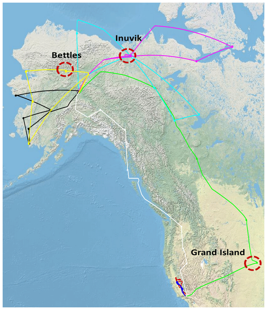
Figure 1Map of flight ground tracks for the 2017 ASCENDS/ABoVE airborne science campaign with NASA DC-8 aircraft (© Google Maps 2019). The colors of the track indicate a total of eight flights from 20 July to 8 August. The three spiral maneuvers are marked with red circles for the three cases described in this study over Grand Island, Nebraska, on 27 July; Inuvik, Northwest Territories of Canada, on 3 August; and Bettles, Alaska, on 6 August.
For this campaign where the measurements were near a spiral-down location, the retrievals used the DC-8 aircraft housekeeping data for the vertical profiles of atmospheric pressure and temperature and water vapor profiles from an onboard engineering test version of the diode laser hygrometer (DLH; Diskin et al., 2002). When co-located radiosonde measurements were available within ± 3 h flight time, the radiosonde data of vertical profiles of atmospheric temperature, pressure and water vapor were used for forward calculations since a radiosonde provides the most accurate data about the vertical structure of the atmospheric state.
There is a weak isotopic water vapor (HDO) line centered at 1572.253 nm on the shoulder of the 1572.335 nm CO2 line. Depending on atmospheric water vapor content, this can distort the CO2 line shape and could significantly impact the value of the XCO2 retrieval. Therefore, the real-time water vapor absorption was calculated and added to CO2 absorption for the best absorption line shape fitting in the retrieval. The XCO2 retrievals were primarily processed based on 1 s averaged lidar data. Since the DC-8 aircraft traveled horizontally at an average speed of 240 m s−1, this resulted in a horizontal resolution of 240 m along the ground track. When the DC-8 aircraft was in a spiral-down maneuver, it descended at 7–8 m s−1.
During July and August 2017, NASA conducted the ASCENDS/ABoVE airborne campaign using the NASA DC-8 aircraft. The flights occurred between 20 July and 8 August 2017 over the ground tracks shown in Fig. 1. In all, eight flights were conducted over the Central Valley of California and over the US Midwest then moved to Fairbanks, AK, and over the Northwest Territories in Canada and over south and central Alaska (Mao et al., 2019, 2021b) before returning to California. This was the first time that airborne XCO2 lidar measurements had been made over the Arctic region.
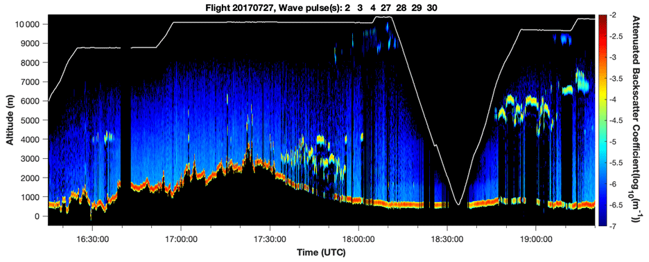
Figure 2Time series of the range-corrected attenuated backscatter profiles measured for the flight over the Rocky Mountains and spiral down over Grand Island, NE, on 27 July 2017. The measurements have 1 s time resolution and a vertical resolution of 15 m. The GPS flight altitudes are marked in a white line, and the ground elevation is shown in the red and yellow band. The lidar returns are averaged for off-line wavelengths or wave pulses nos. 2, 3, 4, 27, 28, 29 and 30 on the wings of the CO2 absorption line. The strong returns from the ground and clouds are colored in yellow and red, while the lidar returns from aerosols and cirrus clouds are weaker and plotted in light blue.
Compared to previous airborne campaigns, the 2017 airborne campaign was conducted in much more dynamic atmosphere conditions over the Northwest Territories of Canada and over Alaska, and it overflew more clouds at multiple levels, as well as smoke plumes from wildfires. The CO2 Sounder lidar continuously measured column absorption of CO2 from the aircraft altitude to the ground and to cloud tops, along with height-resolved backscatter profiles (Sun et al., 2021).
During the campaign, a total of 47 vertical spiral-down maneuvers were conducted over a variety of atmospheres and surface types like desert, vegetation, permafrost, and the Arctic and Pacific Oceans. The purpose of these vertical spiral maneuvers was to compare the lidar XCO2 retrievals with those computed from the onboard in situ CO2 sensors.
The XCO2 retrievals from the lidar measurements were validated against those computed from CO2 vertical profiles measured in situ by the AVOCET sensor (Vay et al., 2011) during the spiral down maneuvers. AVOCET has a stated precision of ± 0.1 ppm (1σ) and an accuracy of ± 0.25 ppm (Halliday et al., 2019). The DC-8 aircraft housekeeping data provided temperature, pressure, geolocation, and positioning such as altitude and pitch or roll angles at flight altitude. The aircraft radar altimeter also provided an independent range measurement to ground under all conditions since the radar measurement penetrates clouds and dense smoke plumes. Using the radar altimeter data with aircraft housekeeping data allows us to calculate the radar-measured surface elevation. This allows distinguishing of the cloud tops from ground or ocean surface in the processing and analysis of the lidar measurements.
Three case studies with spiral-down maneuvers near cloudy regions were selected and analyzed for this study. These are the flight segments over Grand Island, Nebraska, on 27 July; Inuvik, Northwest Territories of Canada, on 3 August; and over Bettles, Alaska, on 6 August.
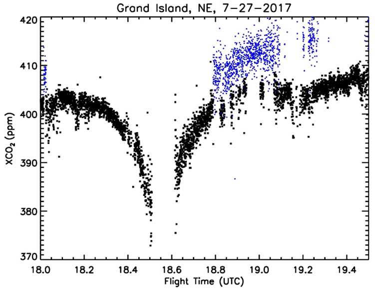
Figure 3Time series of XCO2 retrievals from lidar measurements made surrounding the spiral at Grand Island, NE, on 27 July 2017 using 1 s averaging. The black dots are the retrievals from the lidar measurements to the ground, and the blue dots are those made to the tops of altocumulus clouds.
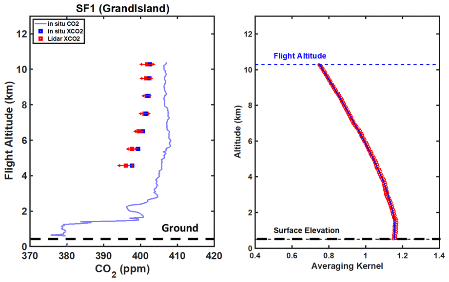
Figure 4Comparison of cloud-free lidar XCO2 retrievals to the ground with those from in situ measurements made during the spiral maneuver at Grand Island, NE, on 27 July 2017. These are computed as a function of flight altitude for averages in every 1 km vertical layer of atmosphere above 4 km. The XCO2 computed from in situ values are marked with blue squares, and the values of the lidar XCO2 retrievals are marked with red squares. The red error bars for the lidar XCO2 retrievals are ± 1 standard deviation. One of the normalized vertical averaging kernels for the lidar XCO2 retrievals for this profile segment is shown on the right. The ground is marked with a thick dashed black line at the bottom, and the flight altitude is marked with a dotted blue line at the top.
4.1 Resolving vertical gradient of atmospheric CO2
We conducted a 9.4 h long south-to-north flight on 27 July 2017, transiting from Palmdale, CA, to Fairbanks, AK. We conducted spiral-down maneuvers at four local airports during the flight. The first spiral-down maneuver had a duration of about 20 min and was conducted over Grand Island, NE, at 18:12 UTC or 1:12 PM local time from a flight altitude of 10 km to near ground. The backscatter profile for this segment of the flights is shown in Fig. 2 and a subsection of the XCO2 in Fig. 3. A very significant drawdown of CO2 (∼ 30 ppm) was observed near the surface at this site; the CO2 mixing ratio at the surface was as low as 376 ppm, while the average CO2 mixing ratio in the free troposphere was 406 ppm (Fig. 4). Some cirrocumulus clouds were near the aircraft altitude prior to the spiral maneuver, while, during the spiral down, the sky was clear. During the flight out from Grand Island, the aircraft flew over altocumulus clouds for about 30 min (18:48–19:18 UTC or 1:48–2:18 PM local time). The cloud top heights of these mid-level clouds ranged from 5 to 7 km, as seen in Fig. 2.
4.1.1 XCO2 measurements to the ground
Figure 4 shows the comparison of lidar XCO2 retrievals to the ground with those from the AVOCET in situ sensor during this spiral-down maneuver. The AVOCET instrument sampled the CO2 mixing ratio outside the aircraft every second. The lidar XCO2 retrievals were based on 1 s averaged lidar data. The in situ XCO2 was computed from the integral of the AVOCET CO2 vertical profile using the vertical averaging kernel of the lidar XCO2 retrieval made from the same altitude. The comparisons were made for averages in every 1 km vertical layer of atmosphere with more than 100 samples as DC-8 aircraft spiraled downward at about 7–8 m s−1.
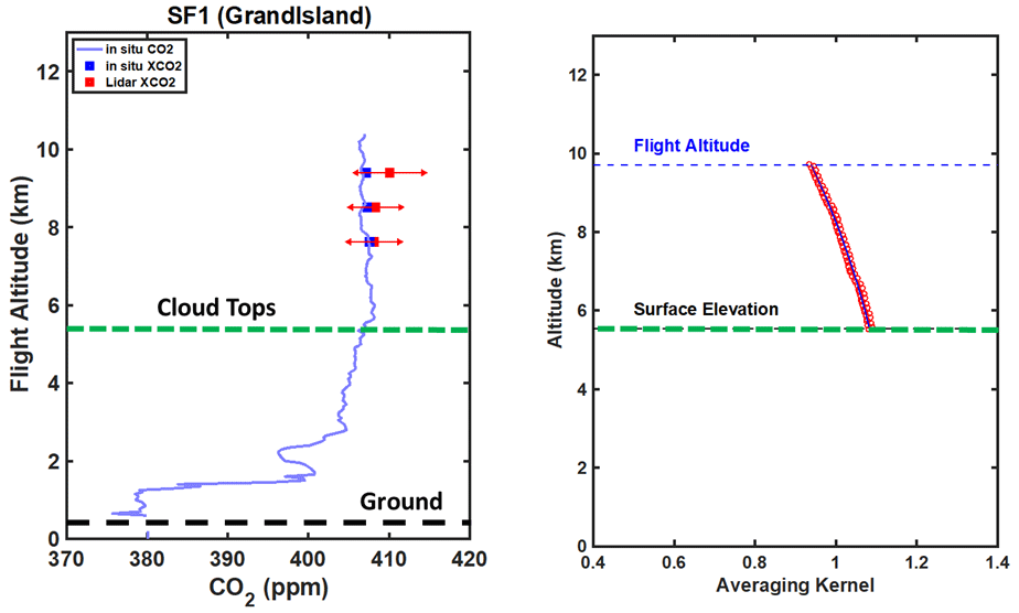
Figure 5Same as Fig. 4 but for the comparison of the lidar XCO2 retrievals to cloud tops with those from in situ measurements during the flight ascent from Grand Island, NE. The ground is marked in a thick dashed black line at the bottom, and the average cloud top height is marked in a thick dashed green line.
As the figure shows, the lidar's averaging kernel peaks in the planetary boundary layer, which means the lidar XCO2 retrievals have the most weighting for CO2 at the bottom atmospheric layers, allowing good sensitivity to surface fluxes. As shown in Fig. 3, there was a significant difference between the lidar XCO2 retrievals made to the ground and those to cloud tops. Both in situ and lidar XCO2 showed a strong vertical gradient, caused by a significant surface drawdown in this area that was covered with growing corn and soybeans crops. When DC-8 aircraft flew away from this area, the lidar-measured XCO2 increased steadily.
The retrievals with the highest precision (lowest standard deviation from the least-squares fit) were from flight altitudes of 7–9 km, indicating the lidar's optimal operating altitude. This optimum is a result of the combined effect of CO2 differential absorption and the number of returned laser photons. At higher flight altitudes, there is more CO2 absorption, but there are fewer received laser photons. This causes a lower signal-to-noise ratio and noisier XCO2 retrievals that have larger standard deviations. At lower flight altitudes the received laser return is greater, but the photon path lengths are shorter, and the CO2 absorption is much weaker, also causing the XCO2 retrievals to have larger standard deviations. The 7–9 km altitude range is where there is the best balance between the line absorption and the number of received signal photons for this instrument.
Compared to the in situ XCO2 from AVOCET, the lidar XCO2 had an average bias of 0.1 ppm for flight altitudes above 5 km. These results are based on 1 s averaged lidar data which typically have a standard deviation of 1.2 ppm. When the lidar data averaging time is increased to 10 s, the standard deviation of lidar XCO2 retrievals to the ground was 0.7 ppm. For 10 s flight time, the length of the aircraft's ground track was typically 2.4 km. The longer averaging time improves the signal-to-noise ratio of the lidar data; however, it also increases the lidar range variation for non-flat surfaces, e.g., vegetation cover and cloud tops, which makes XCO2 retrievals have larger standard deviations (Mao et al., 2018). The overall benefit of a longer data averaging time is to improve the precision of lidar XCO2 retrievals, especially over flat surfaces like deserts and oceans. Longer averaging times also benefit lidar XCO2 retrievals to cloud tops, as shown in the next section.
4.1.2 XCO2 measurements to cloud tops
During the flight out from the Grand Island spiral, the DC-8 flew for about 30 min over extended altocumulus clouds, with cloud top heights between 5 to 7 km. As shown in Fig. 3, the difference between the lidar XCO2 retrievals to the ground and those to cloud tops was significant due to the surface drawdown in this area. As the DC-8 aircraft flew away from this area, the lidar XCO2 increased steadily. Figure 5 shows the comparison of lidar XCO2 retrievals to these mid-level cloud tops during the flight out with those from the in situ vertical profiles of CO2 measured during the spiral-down segment for the flight altitudes above 7 km. The lidar range to cloud tops was between 2 to 4 km. This was shorter than the optimum range for this lidar. From the flight altitudes of 7–9 km, the lidar XCO2 retrievals to cloud tops had an average difference of +0.8 ppm compared to those measured by the in situ sensor during the spiral.
When DC-8 aircraft flew further away from Grand Island, this difference increased to +2.9 ppm. These larger differences are thought to result from significant horizontal differences in the atmosphere (temperature, pressure, water vapor and CO2 profiles) between the region of the spiral-down maneuver and that for the flight-out segment. Note that the optical depth look-up tables of CO2 and H2O used for retrievals were based on the vertical profiles of atmosphere measured during the spiral down. Retrievals of XCO2 to cloud tops during the flight out were made using the same look-up tables for the spiral down. However, the actual conditions are expected to be somewhat different because the atmospheric conditions and CO2 concentrations during summer are expected to have significant gradients in this area.
The retrievals of XCO2 to these cloud tops had a standard deviation of 3–4 ppm for 1 s averaged data, which was about 3 times larger than that for the retrievals to the ground. One reason for this is that the cloud reflectance at the lidar wavelength was typically about 5 %, a factor of 4–5 times lower than that from vegetated surfaces (Mao et al., 2018). Calculations from the lidar data showed that median reflectance of these mid-level clouds at Grand Island was only 2.7 %, while the median value of ground reflectance at Grand Island was 27 %. Additionally, there was less CO2 absorption in the shorter range, and the effects together caused these lidar retrievals to be noisier. In addition, the variability in the elevation of the cloud tops reduces the precision of the XCO2 retrievals. The cloud top altitude used to calculate the photon path length in the retrieval is taken as the centroid of the cloud top altitudes calculated from time-averaged lidar range measurements. These range measurements are averaged over a longer time (1 s or 10 s); the difference in range results in an additional error in the XCO2 retrievals (Mao et al., 2018).
When the data were averaged over 10 s, the standard deviation of XCO2 retrievals to these altocumulus cloud tops at Grand Island improved to 1.3 ppm. This measurement precision for partial column XCO2 to cloud tops is at least 2 times better than those from the 2011, 2013 and 2014 airborne campaigns (Abshire et al., 2014; Mao et al., 2018). This improvement was caused by the utilization of the step-locked seeder laser diode source in the transmitter and the high-sensitivity detector for this campaign (Abshire et al., 2018).
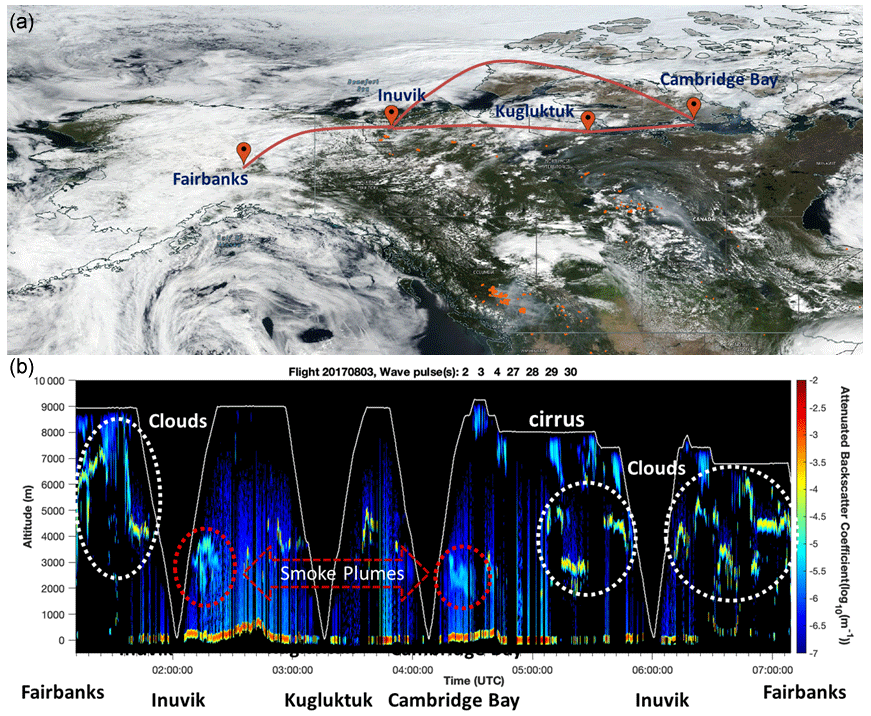
Figure 6True-color image from Aqua/MODIS (a; NASA Worldview) and time series of the lidar's attenuated backscatter profiles (b) for the flight over the Northwest Territories, Canada, on 3 August 2017. Clouds are white, and wildfires are marked with red dots in the MODIS color image. Clouds, including cirrus, and wildfire smoke plumes are circled and labeled in the lidar profiles. The flight ground track is marked in a red line in the top image, and the aircraft GPS flight altitude is marked in a white line in the bottom plot. The locations of spiral maneuvers are labeled. The lidar range-corrected attenuated backscatter profiles were sampled at a vertical resolution of 15 m and averaged over 1 s. Several occurrences of cirrus clouds are clearly seen as light-blue regions just below the aircraft altitude.
4.2 Validation of lidar XCO2 measurements to the tops of mid-level clouds
After the flight from Palmdale, CA, to Fairbanks, AK, we conducted two flights based out of Fairbanks to the Northwest Territories of Canada (NWT). Both flights targeted a northern loop of the area, including the Arctic Ocean. Figure 6 shows the ground track, satellite image and lidar backscatter profiles for the second flight in NWT on 3 August, UTC time. This flight started late on 2 August and went from Fairbanks to Inuvik, then east, then back north along the Arctic Ocean back to Inuvik, then back to Fairbanks. We again used spiral-down maneuvers for comparing the lidar measurements of XCO2 against those from the in situ CO2 profiles above the airports at Inuvik, Kugluktuk, Cambridge Bay, Inuvik again and then Fairbanks.
As shown in Fig. 6, the atmospheric conditions from Fairbanks to Inuvik varied from mostly cloudy to broken clouds at multiple levels on the return leg. These cloud layers provided opportunities for lidar cloud slicing (Ramanathan et al., 2015). There were several occurrences of thick cirrus clouds below the DC-8 aircraft that attenuated the lidar signal and caused some data outages. The path over the Arctic Ocean was also very cloudy, and the vertical structure of the clouds in this path was complex.
Also shown in Fig. 6 are dense smoke plumes from wildfires in the south seen after the spiral-down maneuvers at Inuvik and Cambridge Bay. The atmospheric scattering and attenuation caused by the smoke would significantly degrade or completely screen out any retrievals from passive spectrometers on satellites (Mao and Kawa, 2004; Aben et al., 2007; Butz et al., 2009; Uchino et al., 2012; Guerlet et al., 2013). In contrast, the lidar can accurately measure CO2 enhancements from wildfires through dense smoke plumes, as demonstrated earlier for the large wildfires in the Canadian Rockies during this airborne campaign (Mao et al., 2021a). Measurements of height-resolved atmospheric backscatter profiles allow this lidar approach to accurately estimate XCO2 and range to terrain and water surfaces, even in the presence of wildfire smoke.
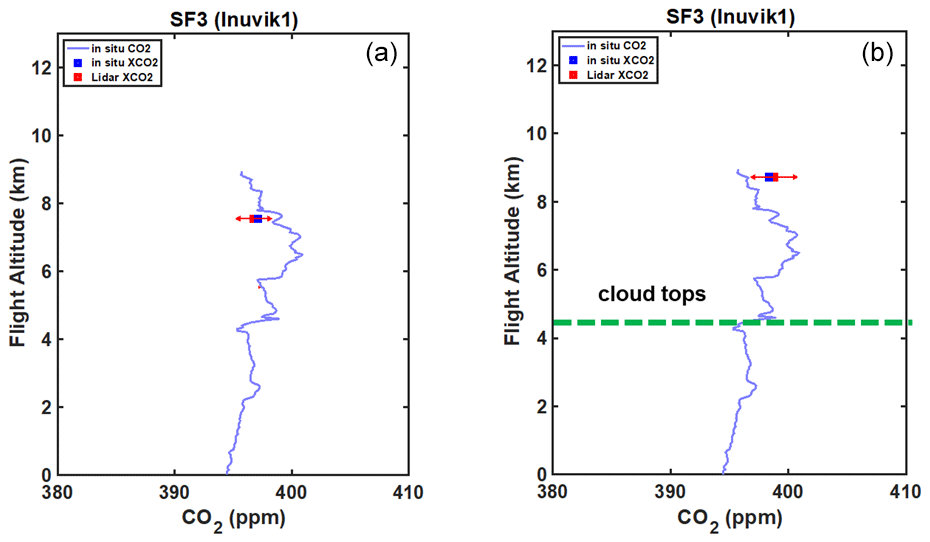
Figure 7Comparison of XCO2 retrievals from lidar measurements made to the ground (a) and to cloud tops (b) during the first spiral-down maneuver at Inuvik, NT, on 3 August 2017. The CO2 profile measured with the in situ sensor is plotted with the blue line. The lidar measurements used a 1 s average. The in situ XCO2 values are marked with blue squares, and the lidar XCO2 retrieval values are marked with red squares. XCO2 values were binned into the top 1 km vertical layer of atmosphere. The red error bars for the lidar XCO2 retrievals are ± 1 standard deviation. In the plot on the right, the average cloud top height is marked as a dashed green line.
During the first spiral-down maneuver of the flight at Inuvik, NT, we overflew some altocumulus clouds with cloud tops around 4.5 (Fig. 6). Figure 7 shows the comparison of both XCO2 retrievals to the ground and to these mid-level cloud tops against those from the in situ CO2 profiles. The measurement local time was around 20:00, and evidence of a small surface sink was noticeable. The differences between the lidar XCO2 retrievals to the ground and to the altocumulus cloud tops were −0.1 and +0.4 ppm, respectively, compared to those from the in situ CO2 profile. The standard deviation of the lidar XCO2 retrievals to the ground from flight altitudes of 7–8 km was 1.3 ppm, while the standard deviation of XCO2 retrievals to cloud tops from flight altitudes of 8–9 km was 1.7 ppm. On average, the lidar range to cloud tops was 4 km for this segment. The lidar measurements showed that the ground reflectance at Inuvik airport was 30 % at the lidar wavelength and that to the tops of the altocumulus clouds was 5.6 %, more than twice that of clouds over Grand Island. This higher reflectance improved the precision of the lidar measurements of XCO2 to these clouds.
These retrieval results were based on 1 s averaged lidar data. When the lidar data averaging time was increased to 10 s, the standard deviation for both retrievals to the ground and to cloud tops decreased to 0.6 ppm. The lidar's measurement precision to cloud tops indicates the benefit of these measurements over persistent cloud cover, which occurs, for example, over the west coasts of continents with marine layered clouds and over the Southern Ocean. These results show that averaging lidar measurements to cloud tops for a longer distance in these regions can fill these significant gaps with high-precision measurements.
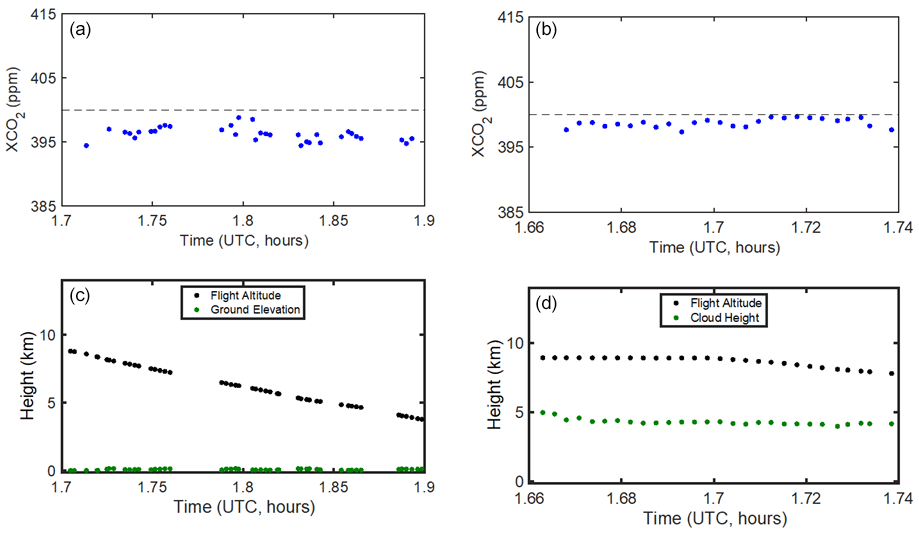
Figure 8XCO2 retrievals from lidar measurements during the spiral-down maneuver at Inuvik, NT, on 3 August 2017, using 10 s averaging. (a) The time series of the XCO2 retrievals made to the ground (blue dots). (c) DC-8 aircraft altitudes and ground elevation for the same segment. Panels (b) and (d) are the same as the left plots but for the lidar XCO2 retrievals made to cloud tops (blue dots). In the lower figures the flight altitudes are plotted with black dots, and the elevation of the ground and cloud tops used for the lidar XCO2 retrievals are plotted with green dots.
Figure 8 shows the time series of the lidar XCO2 retrievals made to the ground and to the altocumulus cloud tops during this spiral down using 10 s data averaging. While the XCO2 measurements to cloud tops were steady during this segment, the measurements to the ground exhibited lower values of XCO2. This small 1.3 ppm difference between these two sets of measurements indicates slightly lower atmospheric carbon below clouds.
4.3 Validation of lidar XCO2 measurements to low-level clouds
Measurements of XCO2 to the ground and to the tops of nearby clouds at the top of the planetary boundary layer provide information to help separate the carbon processes at the Earth's surface from the carbon transport in the free troposphere (Mao et al., 2018; Shi et al., 2021). In earlier airborne campaigns we made measurements to broken cumulus clouds and demonstrated a lidar cloud-slicing approach to estimate partial column XCO2 in the planetary boundary layer (Ramanathan et al., 2015). However, the results from the earlier version of this airborne lidar had larger biases and larger standard deviations even though the lidar data were aggregated over 10 or even 100 s (Abshire et al., 2014; Ramanathan et al., 2015; Mao et al., 2018). The lidar used in the 2017 campaign had several instrument improvements that resulted in improved measurement performance.
After the two flights in the Northwest Territories of Canada, we conducted two flights in southern and central Alaska. On 6 August the flight track went in a counterclockwise direction from Fairbanks westward to Kotzebue, then almost due south and on a diagonal path back toward Fairbanks (Fig. 1). We again used spiral-down maneuvers above the airports at Bettles, Kotzebue, Unalakleet, Platinum, McGrath, Fort Yukon and Fairbanks to validate the lidar XCO2 measurements.
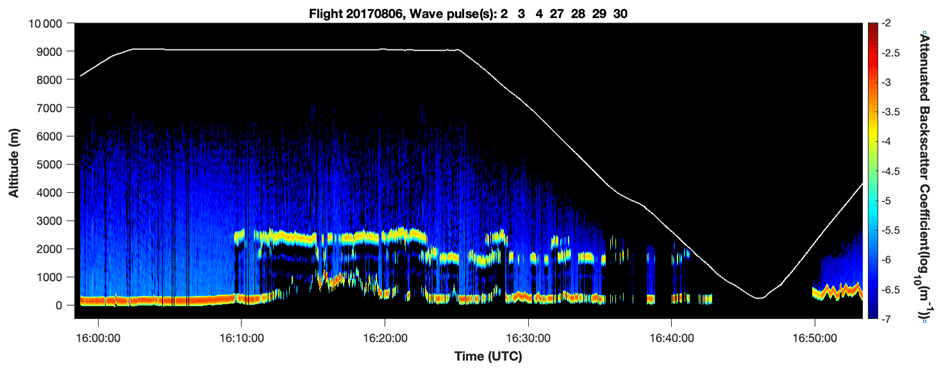
Figure 9Time series of the lidar's range-corrected attenuated backscatter profiles measured for the flight segment over Bettles, AK, on 6 August 2017. The lidar measurements are averaged over 1 s and have a vertical resolution of 15 m. The lidar returns from cloud tops are comparable to those from the ground, as indicated by their red and yellow color scale of the attenuated backscatter coefficients. The aircraft's flight altitude is marked as a white line.
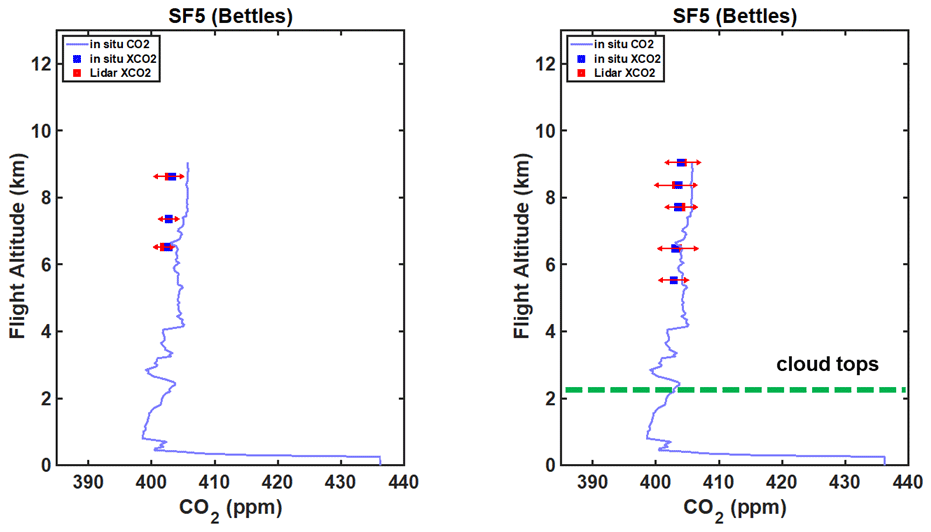
Figure 10XCO2 retrievals from lidar measurements near the spiral down over Bettles, AK, on 6 August 2017. The XCO2 retrieved from 1 s averaged lidar measurements to the ground is on the left, and the lidar XCO2 retrievals to cloud tops are on the right. The CO2 profile measured from the in situ sensor during the spiral-down maneuver is plotted with the blue line. The XCO2 values computed from the in situ measurements are marked with blue squares, and the lidar's XCO2 retrieval values are marked with red squares. XCO2 values were binned into every 1 km vertical layer of atmosphere above 5 km. The red error bars for the lidar retrievals are ± 1 standard deviation. In the plot on the right, the average cloud top height is marked as a dashed green line.
The takeoff time of the 6 August flight was 07:45 local time, and the spiral down at Bettles, AK, started around 08:45 local time or at 16:54 UTC. As shown in Fig. 9, the DC-8 aircraft flew over broken cumulus clouds for about 35 min prior to and during the Bettles spiral down. The heights of cumulus cloud tops ranged from 2 to 2.5 at the top of the planetary boundary layer. As shown in Fig. 10, the in situ sensor showed that the CO2 concentration near the surface was as high as 436 ppm in the morning, which was confined within the lowest 100 m layer. Above that layer the CO2 concentration increased with altitude in the bottom 4 km and remained almost uniform in the upper layers. The XCO2 values measured to the ground and to the tops of cumulus cloud for flight altitudes above 5 km were about the same.
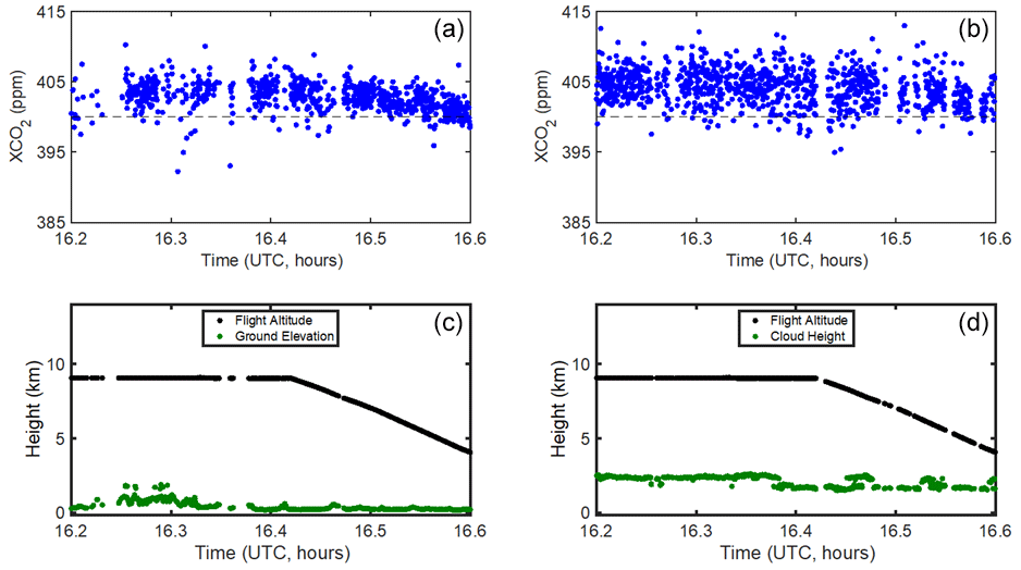
Figure 11Time series of the lidar XCO2 retrievals during the spiral-down maneuver over Bettles, AK, on 6 August 2017. (a) The blue dots are the XCO2 retrievals to the ground for 1 s averaged lidar data. (c) The DC-8 aircraft altitudes and ground elevation. Panels (b) and (d) are the same as the left plots but for the XCO2 retrievals to cloud tops (blue dots). In the lower figures the flight altitudes are plotted with black dots, and the ground elevations and cloud top heights are plotted with green dots.
Figure 10 shows the profile comparison with the in situ measurements. The XCO2 retrievals from lidar measurements to the ground and to the tops of cumulus clouds showed an average bias of +0.2 and −0.4 ppm, respectively, for flight altitudes above 5 km compared to the in situ measurements. The standard deviations of XCO2 measurements to the ground and to cloud tops were 1.5 and 2.5 ppm, respectively, for 1 s average lidar data. In this case, the lidar reflectance of cumulus clouds was 6 %, while the ground reflectance near the Bettles airport was 25 %.
Figure 11 shows the time series of lidar measurements. It shows that the lidar XCO2 retrievals to cloud tops were more scattered than those to the ground, which is mainly caused by the lower reflectance of clouds at the lidar measurement wavelength. Compared to the XCO2 measurements to the mid-level altocumulus cloud tops, the XCO2 measurements to the boundary layer cumulus cloud tops were significantly noisier due to the puffy cumulus cloud tops and the longer range from aircraft to cloud tops (Mao et al., 2018).
When the lidar data are averaged over 10 s, the standard deviation of XCO2 measurements to the ground is 0.8 ppm, and the standard deviation for XCO2 to the cumulus cloud tops is reduced to 0.9 ppm. These lidar XCO2 measurements to the tops of the low-level clouds from the 2017 airborne campaign are 2–3 times better than those from our previous airborne campaigns using the earlier version of the lidar (Mao et al., 2018).
The 2017 ASCENDS/ABoVE airborne campaign was the first time that lidar measurements of XCO2 had been extended to the Arctic region. The summertime Arctic atmosphere contained a variety of cloud types whose tops were at different elevations. These conditions allowed the opportunity to perform lidar XCO2 retrievals to cloud tops and to validate these measurements with those from the onboard in situ sensor during spiral-down maneuvers.
The results showed that the standard deviation of the lidar XCO2 retrievals to cloud tops for 1 s average data from this campaign was equivalent to that for 10 s average data from previous campaigns in 2011, 2013 and 2014. The improvement in data precision for this campaign enabled the utilization of a step-locked seeder laser diode source and the higher-sensitivity lidar detector.
When the data averaging time was increased to 10 s, the standard deviations of the lidar retrievals improved to 0.6 ppm for the mid-level clouds and 0.9 ppm for the low-level clouds at the top of the planetary boundary layer. The precision of XCO2 measurements to cloud tops was typically 2–3 times lower than those to the ground due to the lower reflectance of clouds at the 1572 nm lidar wavelength. During the 2017 airborne campaign, most flight altitudes were below 10 km, and so the lidar ranges to cloud tops were relatively short. There were many occurrences of cirrus clouds during the flights; however, the ranges from the aircraft to the tops of these cirrus clouds were short, resulting in weak CO2 absorption and poor retrievals. For future space-based lidar measurements, the longer atmospheric path length to cirrus clouds should allow useful XCO2 measurements to cirrus clouds as well.
These results indicate the significant benefit of the lidar's measurements to cloud tops, particularly those made over persistent cloud cover, e.g., the Intertropical Convergence Zone, the western coasts of continents with marine layered clouds, the Southern Ocean with low-level clouds and the Arctic. These are important areas with active carbon cycling but where measurements from passive satellite-based spectrometers are sparse or unavailable.
This study demonstrated that this lidar's XCO2 measurements to cloud tops, along with those to the ground, can be used to help resolve vertical and horizontal gradients of CO2. This lidar capability can be used to fill significant measurement gaps left by passive spectrometer missions and to help resolve the vertical distribution of atmospheric CO2. Future airborne campaigns and spaceborne missions with this lidar's measurement capability, like NASA's planned ASCENDS mission (Kawa et al., 2018), would improve carbon data assimilation, atmospheric transport modeling and flux estimation and would advance carbon cycle science.
The lidar XCO2 retrievals for the clear sky from the 2017 airborne campaign are available from the NASA Airborne Science Data for Atmospheric Composition website, https://www-air.larc.nasa.gov/cgi-bin/ArcView/ascends.2017#ABSHIRE.JAMES/ (NASA Langley Research Center, 2020). The lidar XCO2 retrievals to cloud tops used in this work are available from the primary authors.
JM led the paper writing and the airborne campaign data processing and analysis. JBA was the principal investigator of the CO2 Sounder lidar development, led the 2017 ASCENDS/ABoVE airborne campaign, and contributed to the analysis and paper. SRK contributed to the 2017 airborne campaign, the campaign data processing and analysis, and the paper editing. XS contributed to the CO2 Sounder lidar development, the lidar data analysis and the paper editing. HR contributed to the CO2 Sounder lidar development, the 2017 airborne campaign, and the campaign data processing and analysis.
The contact author has declared that none of the authors has any competing interests.
Publisher's note: Copernicus Publications remains neutral with regard to jurisdictional claims made in the text, published maps, institutional affiliations, or any other geographical representation in this paper. While Copernicus Publications makes every effort to include appropriate place names, the final responsibility lies with the authors.
We appreciate the work of Graham Allan, Kenji Numata and Jeffrey Chen from NASA Goddard Space Flight Center in supporting the CO2 Sounder lidar, as well as Joshua P. DiGangi, Glenn Diskin and Yonghoon Choi from NASA Langley Research Center for participating in the airborne campaign and for providing the in situ CO2 and H2O data. We gratefully acknowledge the work of the DC-8 aircraft team at NASA's Armstrong Flight Center in helping to plan and conduct the flight campaign. We thank Paul T. Kolbeck from the University of Maryland at College Park for the lidar backscatter data processing. We acknowledge the use of imagery from the NASA Worldview application (https://worldview.earthdata.nasa.gov/, last access: 25 April 2023), part of the NASA Earth Observing System Data and Information System (EOSDIS). We also would like to thank two anonymous reviewers for their helpful reviews and recommendations.
This research was supported by the NASA ABoVE project, the NASA ASCENDS mission pre-formulation activity, the NASA Earth Sciences Technology Office and NASA's Airborne Science Program.
This paper was edited by Christoph Kiemle and reviewed by two anonymous referees.
Aben, I., Hasekamp, O., and Hartmann, W.: Uncertainties in the space-based measurements of CO2 columns due to scattering in the Earth's atmosphere, J. Quant. Spectrosc. Ra., 104, 450–459, 2007.
Abshire, J. B., Riris, H., Allan, G. R., Weaver, C. J., Mao, J., Sun, X., Hasselbrack, W. E., Kawa, S. R., and Biraud, S.: Pulsed airborne lidar measurements of atmospheric CO2 column absorption, Tellus, 62, 770–783, 2010.
Abshire, J. B., Riris, H., Weaver, C. W., Mao, J., Allan, G. R., Hasselbrack, W. E., Weaver, C. J., and Browell, E. W.: Airborne measurements of CO2 column absorption and range using a pulsed direct-detection integrated path differential absorption lidar, Appl. Optics, 52, 4446–4461, 2013.
Abshire, J. B., Ramanathan, A., Riris, H., Mao, J., Allan, G. R., Hasselbrack, W. E., Weaver, C. J., and Browell, E. W.: Airborne Measurements of CO2 Column Concentration and Range using a Pulsed Direct-Detection IPDA Lidar, Remote Sens., 6, 443–469; https://doi.org/10.3390/rs6010443, 2014.
Abshire, J. B., Ramanathan, A. K., Riris, H., Allan, G. R., Sun, X., Hasselbrack, W. E., Mao, J., Wu, S., Chen, J., Numata, K., Kawa, S. R., Yang, M. Y. M., and DiGangi, J.: Airborne measurements of CO2 column concentrations made with a pulsed IPDA lidar using a multiple-wavelength-locked laser and HgCdTe APD detector, Atmos. Meas. Tech., 11, 2001–2025, https://doi.org/10.5194/amt-11-2001-2018, 2018.
Amediek, A., Sun, X., and Abshire, J. B.: Analysis of range measurements from a pulsed airborne CO2 integrated path differential absorption lidar, IEEE T. Geosci. Remote, 51, 2498–2504, 2013.
Borsdorff, T., Hasekamp, O. P., Wassmann, A., and Landgraf, J.: Insights into Tikhonov regularization: application to trace gas column retrieval and the efficient calculation of total column averaging kernels, Atmos. Meas. Tech., 7, 523–535, https://doi.org/10.5194/amt-7-523-2014, 2014.
Butz, A., Hasekamp, O. P., Frankenberg, C., and Aben, I.: Retrievals of atmospheric CO2 from simulated space-borne measurements of backscattered near-infrared sunlight: accounting for aerosol effects, Appl. Optics, 48, 3322–3336, 2009.
Chevallier, F., Palmer, P. I., Feng, L., Boesch, H., O'Dell, C. W., and Bousquet, P.: Toward robust and consistent regional CO2 flux estimates from in situ and spaceborne measurements of atmospheric CO2, Geophys. Res. Lett., 41, 1065–1070, https://doi.org/10.1002/2013GL058772, 2014.
Clough, S. A. and Iacono, M. J.: Line-by-line calculation of atmospheric fluxes and cooling rates 2. Application to carbon dioxide, methane, nitrous oxide, and halocarbons. J. Geophys. Res.-Atmos. 100, 16519–16535, 1995.
Clough, S. A., Iacono, M. J., and Moncet, J.: Line-by-line calculations of atmospheric fluxes and cooling rates: Application to water vapor, J. Geophys. Res.-Atmos., 97, 15761–15785, 1992.
Crisp, D., Atlas, R. M., Breon, F.-M., Brown, L. R., Burrows, J. P., Ciais, P., Connor, B. J., Doney, S. C., Fung, I. Y., Jacob, D. J., Miller, C. E., O'Brien, D., Pawson, S., Randerson, J. T., Rayner, P., Salawitch, R. J., Sander, S. P., Sen, B., Stephens, G. L., Tans, P. P., Toon, G. C., Wennberg, P. O., Wofsy, S. C., Yung, Y. L., Kuang, Z., Chudasama, B., Sprague, G., Weiss, B., Pollock, R., Kenyon, D., and Schroll, S.: The Orbiting Carbon Observatory (OCO) Mission, Adv. Space Res., 34, 700–709, 2004.
Diskin, G. S., Podolske, J. R., Sachse, G. W., and Slate, T. A.: Open-path airborne tunable diode laser hygrometer, in: Proc. SPIE 4817, Diode Lasers and Applications in Atmospheric Sensing, Seattle, WA, USA, 23 September 2002, https://doi.org/10.1117/12.453736, 2002.
Feng, L., Palmer, P. I., Bösch, H., and Dance, S.: Estimating surface CO2 fluxes from space-borne CO2 dry air mole fraction observations using an ensemble Kalman Filter, Atmos. Chem. Phys., 9, 2619–2633, https://doi.org/10.5194/acp-9-2619-2009, 2009.
Feng, L., Palmer, P. I., Parker, R. J., Deutscher, N. M., Feist, D. G., Kivi, R., Morino, I., and Sussmann, R.: Estimates of European uptake of CO2 inferred from GOSAT retrievals: sensitivity to measurement bias inside and outside Europe, Atmos. Chem. Phys., 16, 1289–1302, https://doi.org/10.5194/acp-16-1289-2016, 2016.
Feng, L., Palmer, P. I., Bösch, H., Parker, R. J., Webb, A. J., Correia, C. S. C., Deutscher, N. M., Domingues, L. G., Feist, D. G., Gatti, L. V., Gloor, E., Hase, F., Kivi, R., Liu, Y., Miller, J. B., Morino, I., Sussmann, R., Strong, K., Uchino, O., Wang, J., and Zahn, A.: Consistent regional fluxes of CH4 and CO2 inferred from GOSAT proxy XCH4:XCO2 retrievals, 2010–2014, Atmos. Chem. Phys., 17, 4781–4797, https://doi.org/10.5194/acp-17-4781-2017, 2017.
Guerlet, S., Butz, A., Schepers, D., Basu, S., Hasekamp, O. P., Kuze, A., Yokota, T., Blavier, J.-F., Deutscher, N. M., Griffith, D. W. T., Hase, F., Kyro, E., Morino, I., Sherlock, V., Sussmann, R., Galli, A., and Aben, I.: Impact of aerosol and thin cirrus on retrieving and validating XCO2 from GOSAT shortwave infrared measurements, J. Geophys. Res., 118, 4887–4905, https://doi.org/10.1002/jgrd.50332, 2013.
Halliday, H. S., DiGangi, J. P., Choi, Y., Diskin, G. S., Pusede, S. E., Rana, M., Nowak, J. B., Knote, C., Ren, X., He, H., Dickerson, R. R., and Li, Z.: Using short-term ratios to assess air mass differences over the Korean Peninsula during KORUS-AQ, J. Geophys. Res.-Atmos., 124, 10951–10972, https://doi.org/10.1029/2018JD029697, 2019.
Kawa, S. R., Mao, J., Abshire, J. B., Collatz, G. J., Sun, X., and Weaver, C. J.: Simulation studies for a space-based CO2 lidar mission, Tellus B, 62, 770–783, https://doi.org/10.1111/j.1600-0889.2010.00486.x, 2010.
Kawa, S. R., Abshire, J. B., Baker, D. F., Browell, E. V., Crisp, D., Crowell, S. M. R., Hyon, J. J., Jacob, J. C., Jucks, K. W., Lin, B., Menzies, R. T., Ott, L. E., and Zaccheo, T. S.: Active Sensing of CO2 Emissions over Nights, Days, and Seasons (ASCENDS): Final Report of the ASCENDS, Ad Hoc Science Definition Team, Document ID: 20190000855, NASA/TP–2018-219034, GSFC-E-DAA-TN64573, https://www-air.larc.nasa.gov/missions/ascends/docs/NASA_TP_2018-219034_ASCENDS_ID1.pdf (last access: 14 May 2021), 2018.
Kuze, A., Suto, H., Nakajima, M., and Hamazaki, T.: Thermal and near infrared sensor for carbon observation Fourier-transform spectrometer on the greenhouse gases observing satellite for greenhouse gases monitoring, Appl. Optics, 48, 6716–6733, 2009.
Mao, J. and Kawa, S. R.: Sensitivity studies for space-based measurement of atmospheric total column carbon dioxide by reflected sunlight, Appl. Optics, 43, 914–927, 2004.
Mao, J., Ramanathan, A., Abshire, J. B., Kawa, S. R., Riris, H., Allan, G. R., Rodriguez, M., Hasselbrack, W. E., Sun, X., Numata, K., Chen, J., Choi, Y., and Yang, M. Y. M.: Measurement of atmospheric CO2 column concentrations to cloud tops with a pulsed multi-wavelength airborne lidar, Atmos. Meas. Tech., 11, 127–140, https://doi.org/10.5194/amt-11-127-2018, 2018.
Mao, J., Abshire, J. B., Kawa, S. R., Riris, H., Allan, G. R., Hasselbrack, W. E., Sun, X., Chen, J., Numata, K., Sun, X., Nicely, J. M., GiGang, J. P., and Choi, Y.: CO2 Laser Sounder Lidar: Toward Atmospheric CO2 Measurements with High-precision, Low-bias and Global coverage, A43D-01 presented at the Fall Meeting, AGU, San Francisco, CA, 9–13 December 2019, https://agu.confex.com/agu/fm19/meetingapp.cgi/Paper/540584 (last access: 24 January 2024), 2019.
Mao, J., Abshire, J. B., Kawa, S. R., Riris, H., Sun, X., Andela, N., and Kolbeck, P. T.: Measuring Atmospheric CO2 Enhancements from the 2017 British Columbia using a Lidar, Geophys. Res. Lett., 48, e2021GL093805. https://doi.org/10.1029/2021GL093805, 2021a.
Mao, J., Abshire, J. B., Kawa, S. R., Riris, H., Sun, X., Nicely , J. M., and Kolbeck, P. T.: The NASA Goddard CO2 Sounder Lidar: 2017 Airborne Campaign as a Demonstration toward a Future Space Mission, 2021 IEEE International Geoscience and Remote Sensing Symposium IGARSS, Brussels, Belgium, 11–16 July 2021, https://doi.org/10.1109/IGARSS47720.2021.9554611, pp. 1673–1676, 2021b.
NASA Langley Research Center: Airborne Science Data for Atmospheric Composition, DC-8 Aircraft Data, https://www-air.larc.nasa.gov/cgi-bin/ArcView/ascends.2017#ABSHIRE.JAMES/ (last access: 16 May 2021), 2020.
Numata, K., Chen, J. R., Wu, S. T., Abshire, J. B., and Krainak, M. A.: Frequency stabilization of distributed-feedback laser diodes at 1572 nm for lidar measurements of atmospheric carbon dioxide, Appl. Optics, 50, 1047–1056, 2011.
Numata, K., Chen, J. R., and Wu, S. T.: Precision and fast wavelength tuning of a dynamically phase-locked widely-tunable laser, Opt. Express, 20, 14234–14243, https://doi.org/10.1364/OE.20.014234, 2012.
Palmer, P. I., Wilson, E. L., L. Villanueva, G., Liuzzi, G., Feng, L., DiGregorio, A. J., Mao, J., Ott, L., and Duncan, B.: Potential improvements in global carbon flux estimates from a network of laser heterodyne radiometer measurements of column carbon dioxide, Atmos. Meas. Tech., 12, 2579–2594, https://doi.org/10.5194/amt-12-2579-2019, 2019.
Ramanathan, A., Mao, J., Allan, G. R., Riris, H., Weaver, C. J., Hasselbrack, W. E., Browell, E. V., and Abshire, J. B.: Spectroscopic measurements of a CO2 absorption line in an open vertical path using an airborne lidar, Appl. Phys. Lett., 103, 214102, https://doi.org/10.1063/1.4832616, 2013.
Ramanathan, A., Mao, J., Abshire, J. B., and Allan, G. R.: Remote sensing measurements of the CO2 mixing ratio in the Planetary Boundary Layer using Cloud Slicing with Airborne Lidar, Geophys. Res. Lett., 42, 2055–2062, https://doi.org/10.1002/2014GL062749, 2015.
Ramanathan, A. K., Nguyen, H. M., Sun, X., Mao, J., Abshire, J. B., Hobbs, J. M., and Braverman, A. J.: A singular value decomposition framework for retrievals with vertical distribution information from greenhouse gas column absorption spectroscopy measurements, Atmos. Meas. Tech., 11, 4909–4928, https://doi.org/10.5194/amt-11-4909-2018, 2018.
Reuter, M., Buchwitz, M., Hilker, M., Heymann, J., Schneising, O., Pillai, D., Bovensmann, H., Burrows, J. P., Bösch, H., Parker, R., Butz, A., Hasekamp, O., O'Dell, C. W., Yoshida, Y., Gerbig, C., Nehrkorn, T., Deutscher, N. M., Warneke, T., Notholt, J., Hase, F., Kivi, R., Sussmann, R., Machida, T., Matsueda, H., and Sawa, Y.: Satellite-inferred European carbon sink larger than expected, Atmos. Chem. Phys., 14, 13739–13753, https://doi.org/10.5194/acp-14-13739-2014, 2014.
Rothman, L. S., Gordon, I. E., Barbe, A., Chris Benner, D., Bernath, P. F., Birk, M., Boudon, V., Brown, L. R., Campargue, A., Champion, J.-P., Chance, K., Coudert, L. H., Dana, V., Devi, V. M., Fally, S., Flaud, J.-M., Gamache, R. R., Goldman, A., Jacquemart, D., Kleiner, I., Lacome, N., Lafferty, W. J., Mandin, J.-Y., Massie, S. T., Mikhailenko, S. N., Miller, C. E., Moazzen-Ahmadi, N., Naumenko, O. V., Nikitin, A. V., Orphal, J., Perevalov, V. I., Perrin, A., Predoi-Cross, A., Rinsland, C. P., Rotger, M., Šimeková, M., Smith, M. A. H., Sung, K., Tashkun, S. A., Tennyson, J., Toth, R. A., Vandaele, A. C., and Vander Auwera, J.: The HITRAN 2008 molecular spectroscopic database, J. Quant. Spectrosc. Ra., 110, 533–572, 2009.
Schimel, D., Sellers, P., Moore III, B., Chatterjee, A., Baker, D., Berry, J., Bowman, K., Ciais, P., Crisp, D., Crowell, S., Denning, S., Duren, R., Friedlingstein, P., Gierach, M., Gurney, K., Hibbard, K., Houghton, R. A., Huntzinger, D., Hurtt, G., Jucks, K., Kawa, R., Koster, R., Koven, C., Luo, Y., Masek, J., McKinley, G., Miller, C., Miller, J., Moorcroft, P., Nassar, R., O’Dell, C., Ott, L., Pawson, S., Puma, M., Quaife, T., Riris, H., Romanou, A., Rousseaux, C., Schuh, A., Shevliakova, E., Tucker, C., Wang, Y. P., Williams, C., Xiao, X., and Yokota, T.: Observing the carbon-climate system, arXiv [physics.ao-ph], arXiv:1604.02106v1, 2016.
Shi, T., Han, G., Ma, X., Gong, W., Chen, W., Liu, J., Zhang, X., Pei, Z., Gou, H., and Bu, L.: Quantifying CO2 uptakes over oceans using LIDAR: A tentative experiment in Bohai Bay, Geophys. Res. Lett., 48, e2020GL091160, https://doi.org/10.1029/2020GL091160, 2021.
Sun, X., Abshire, J. B., Beck, J. D., Mitra, P., Reiff, K., and Yang, G.: HgCdTe avalanche photodiode detectors for airborne and spaceborne lidar at infrared wavelengths, Opt. Express, 25, 16589–16602, https://doi.org/10.1364/OE.25.016589, 2017.
Sun, X., Abshire, J. B., Ramanathan, A., Kawa, S. R., and Mao, J.: Retrieval algorithm for the column CO2 mixing ratio from pulsed multi-wavelength lidar measurements, Atmos. Meas. Tech., 14, 3909–3922, https://doi.org/10.5194/amt-14-3909-2021, 2021.
Sun, X., Kolbeck, P. T., Abshire, J. B., Kawa, S. R., and Mao, J.: Attenuated atmospheric backscatter profiles measured by the CO2 Sounder lidar in the 2017 ASCENDS/ABoVE airborne campaign, Earth Syst. Sci. Data, 14, 3821–3833, https://doi.org/10.5194/essd-14-3821-2022, 2022.
Uchino, O., Kikuchi, N., Sakai, T., Morino, I., Yoshida, Y., Nagai, T., Shimizu, A., Shibata, T., Yamazaki, A., Uchiyama, A., Kikuchi, N., Oshchepkov, S., Bril, A., and Yokota, T.: Influence of aerosols and thin cirrus clouds on the GOSAT-observed CO2: a case study over Tsukuba, Atmos. Chem. Phys., 12, 3393–3404, https://doi.org/10.5194/acp-12-3393-2012, 2012.
Vay, S. A., Choi, Y., Vadrevu, K. P., Blake, D. R., Tyler, S. C., Wisthaler, A., Hecobian, A., Kondo, Y., Diskin, G. S., Sachse, G. W., Woo, J. H., Weinheimer, A. J., Burkhart, J. F., Stohl, A., and Wennberg, P. O.: Patterns of CO2 and radiocarbon across high northern latitudes during International Polar Year 2008, J. Geophys. Res.-Atmos., 116, D14301, https://doi.org/10.1029/2011JD015643, 2011.
Vekuri, H., Tuovinen, J. P., Kulmala, L. Papale, D., Kolari, P., Aurela, M., Laurila, T., Liski, J., and Lohila, A.: A widely used eddy covariance gap-filling method creates systematic bias in carbon balance estimates, Sci. Rep.-UK, 13, 1720, https://doi.org/10.1038/s41598-023-28827-2, 2023.
Wunch, D., Toon, G. C., Blavier, J.-F. L., Washenfelder, R. A., Notholt, J., Connor, B. J., Griffith, D. W. T., Sherlock, V., and Wennberg, P. O.: The total carbon column observing network, Philos. T. R. Soc. A, 369, 2087–2112, https://doi.org/10.1098/rsta.2010.0240, 2011.