Profiling the molecular destruction rates of temperature and humidity as well as the turbulent kinetic energy dissipation in the convective boundary layer

A simultaneous deployment of Doppler, temperature, and water-vapor lidars is able to provide profiles of molecular destruction rates and turbulent kinetic energy (TKE) dissipation in the convective boundary layer (CBL). Horizontal wind profiles and profiles of vertical wind, temperature, and moisture fluctuations are combined, and transversal temporal autocovariance functions (ACFs) are determined for deriving the dissipation and molecular destruction rates. These are fundamental loss terms in the TKE as well as the potential temperature and mixing ratio variance equations. These ACFs are fitted to their theoretical shapes and coefficients in the inertial subrange. Error bars are estimated by a propagation of noise errors. Sophisticated analyses of the ACFs are performed in order to choose the correct range of lags of the fits for fitting their theoretical shapes in the inertial subrange as well as for minimizing systematic errors due to temporal and spatial averaging and micro- and mesoscale circulations. We demonstrate that we achieve very consistent results of the derived profiles of turbulent variables regardless of whether 1 or 10 s time resolutions are used. We also show that the temporal and spatial length scales of the fluctuations in vertical wind, moisture, and potential temperature are similar with a spatial integral scale of ≈160 m at least in the mixed layer (ML). The profiles of the molecular destruction rates show a maximum in the interfacial layer (IL) and reach values of ${\mathit{ϵ}}_m\simeq \mathrm{7}\times {\mathrm{10}}^{-\mathrm{4}}$ g² kg⁻² s⁻¹ for mixing ratio and ${\mathit{ϵ}}_{\mathit{\theta }}\simeq \mathrm{1.6}\times {\mathrm{10}}^{-\mathrm{3}}$ K² s⁻¹ for potential temperature. In contrast, the maximum of the TKE dissipation is reached in the ML and amounts to $\simeq {\mathrm{10}}^{-\mathrm{2}}$ m² s⁻³. We also demonstrate that the vertical wind ACF coefficient $k_w\propto \stackrel{\mathrm{‾}}{{w^{\prime }}^{\mathrm{2}}}$ and the TKE dissipation $\mathit{ϵ}\propto {\left(\stackrel{\mathrm{‾}}{{w^{\prime }}^{\mathrm{2}}}\right)}^{\mathrm{3}/\mathrm{2}}$. For the molecular destruction rates, we show that ${\mathit{ϵ}}_m\propto \stackrel{\mathrm{‾}}{{m^{\prime }}^{\mathrm{2}}}{\left(\stackrel{\mathrm{‾}}{{w^{\prime }}^{\mathrm{2}}}\right)}^{\mathrm{1}/\mathrm{2}}$ and ${\mathit{ϵ}}_{\mathit{\theta }}\propto \stackrel{\mathrm{‾}}{{{\mathit{\theta }}^{\prime }}^{\mathrm{2}}}{\left(\stackrel{\mathrm{‾}}{{w^{\prime }}^{\mathrm{2}}}\right)}^{\mathrm{1}/\mathrm{2}}$. These equations can be used for parameterizations of ϵ, ϵ_m, and ϵ_θ. All noise error bars are derived by error propagation and are small enough to compare the results with previous observations and large-eddy simulations. The results agree well with previous observations but show more detailed structures in the IL. Consequently, the synergy resulting from this new combination of active remote sensors enables the profiling of turbulent variables such as integral scales, variances, TKE dissipation, and the molecular destruction rates as well as deriving relationships between them. The results can be used for the parameterization of turbulent variables, TKE budget analyses, and the verification of large-eddy simulations.

1 Introduction

Improved understanding and modeling of turbulent transport processes in the convective boundary layer (CBL) require in-depth studies of the budgets of second- and other higher-order moments of atmospheric variables. Key variables include turbulent kinetic energy (TKE) and water-vapor and temperature variances; the latter is in terms of absolute humidity, mixing ratio, or specific humidity variances as well as temperature or potential temperature variances. The analysis of TKE and variance budgets and their components is important for the verification of weather forecast, climate, and Earth system models. Furthermore, the representation of budgets of second-order moments of atmospheric variables is essential for the parameterization of turbulent transport processes in mesoscale models, in which the turbulence is not explicitly resolved, or for the parameterization of subgrid-scale cloud processes.

In a turbulent flow, eddy diameters span a range of length scales (Tennekes and Lumley, 1972). For a turbulent boundary layer, the largest eddies, which have the largest velocity fluctuations and thus the largest contributions to the velocity variances and the TKE, generally scale with the depth of that layer. These large eddies break down into smaller and smaller eddies. Although the resulting small eddies contribute less to the variances and have much less energy, they are important because when they get small enough, the fluctuations are damped by molecular viscosity in such a way that they become the major sink for TKE in the budget equation. We refer to this sink as the molecular destruction of variances or dissipation of TKE. The sources of turbulence thus occur at the largest turbulent scales, but the sink of the turbulence is at the smallest scales. Whether TKE increases or decreases depends on the balance between the sources and the sink, so establishing the magnitude of the sink is key to proper modeling of turbulent mixing effects. A common approach to turbulence parameterization (TP) in mesoscale numerical weather prediction (NWP) models is to solve budget equations for TKE and other scalar variances, presented later in this paper. This procedure requires predictive equations for those variances, including temperature (or potential temperature) and water-vapor specific humidity or mixing ratio. As is the case for TKE, the generation of scalar variance occurs at larger turbulence scales, but the major sink is due to molecular damping or “destruction” at the smallest scales. These rates must be parameterized in mesoscale NWP models.

Large-eddy and direct numerical simulation (LES and DNS) models predict turbulence fields by explicitly resolving turbulent processes into the inertial subrange. Resolving these processes avoids the need for TPs at their spatial grid increments (​​​​​​​⪅​​​​​​​ 100 m), but it is still necessary to parameterize the remaining subgrid-scale processes, such as the TKE dissipation and molecular destruction rates. Therefore, from the mesoscale to the turbulent scale, vertical profiling of TKE dissipation and destruction rates of molecular variances are very useful. On the mesoscale, these measurements can be used for the verification of TPs. On the smaller scales, these observations are very important for the verification of the performance of LES and DNS.

This verification should be performed under a range of different meteorological conditions, from the surface layer (SL), through the mixed layer (ML) and the interfacial layer (IL) at the CBL top to the lower troposphere. Previous studies, as early as the 1970s, mainly used in situ measurements (Caughey and Palmer, 1979; Lenschow et al., 1980). These sensors were operated on research aircraft; in the future, it should also be possible to perform these measurements on unoccupied aerial vehicles (UAVs). However, turbulence measurements from aircraft and UAVs are limited with respect to duration and vertical range, and there can be questions as to where the observations are located relative to the CBL top (Turner et al., 2014a). Furthermore, it is difficult to measure instantaneous vertical profiles of mean and turbulent variables, thereby limiting their applications for process studies and model verification.

A powerful alternative is the operation and application of ground-based active remote systems, which are considered in this work. In the SL, scanning lidar systems were successfully combined to derive high-resolution profiles for studying Monin–Obukhov similarity theory (Späth et al., 2022), but close to the surface, the temporal–spatial resolutions of the lidar systems are not sufficient to resolve the major part of the turbulent fluctuations. Due to recent technological advances, Doppler lidar (DL) systems are now available for $\mathrm{24}/\mathrm{7}$ measurements of horizontal and vertical wind profiles in the CBL. The range and time resolutions of line-of-sight (LOS) velocity measurements with DLs are high enough to resolve turbulent processes above the SL from the ML to the IL. Recently, it has been demonstrated that conically scanning DLs are capable of measuring horizontal wind profiles with high vertical and temporal resolutions as well as accuracy (Berg et al., 2017). Six-beam staring modes of DLs have been developed with even greater information content, as TKE, momentum flux, and horizontal wind profiles can be determined simultaneously (Bonin et al., 2017). Furthermore, vertically staring DLs have been extensively used for the measurement of vertical wind (w) statistics (Lenschow et al., 2000; Wulfmeyer and Janjić, 2005; Hogan et al., 2009; Lothon et al., 2009; Tucker et al., 2009; Ansmann et al., 2010; Lenschow et al., 2012) and TKE dissipation profiles (Frehlich and Cornman, 2002; O'Connor et al., 2010; Banakh et al., 2017; Bodini et al., 2018; Wildmann et al., 2019).

For the measurement of scalar variances and their destruction rates, high-resolution vertical profiling of temperature and moisture is also possible with active remote sensing. Sufficient spatial–temporal resolutions can be reached with water-vapor differential absorption lidar (WVDIAL) and water-vapor Raman lidar (WVRL). For WVDIAL, this was demonstrated in Wulfmeyer (1999), Lenschow et al. (2000), Späth et al. (2016), Muppa et al. (2016), and Wulfmeyer et al. (2016). For WVRL, this performance was confirmed in Wulfmeyer et al. (2010), Turner et al. (2014a, b), Wulfmeyer et al. (2018), and Osman et al. (2019).

With respect to temperature measurements, a breakthrough has recently been achieved using the temperature rotational Raman lidar (TRRL) technique. The first demonstration of high-resolution temperature profiling during daytime in the CBL, from which higher-order moments could be derived, was presented in Hammann et al. (2015) and Behrendt et al. (2015). Similarly to this work, these publications were based on High Definition Clouds and Precipitation (HD(CP)²) Observational Prototype Experiment (HOPE) (Macke et al., 2017) data. The first combined measurements of sensible and latent heat flux profiles can be found in Behrendt et al. (2020). Furthermore, Lange et al. (2019) showed that by using a compact design, even quasi-operational measurements down to a vertical resolution of 7.5 m and a temporal resolution of 10 s are possible so that it is straightforward to analyze temperature variance profiles in the daytime CBL. Therefore, the combination of DL, WVRL or WVDIAL, and TRRL can be used for extensive turbulence studies based on their single profiles or a combination of these. Further details about the combined WV and T Raman lidar methodology are found in Wulfmeyer and Behrendt (2021).

DL measurements are available from observatories such as the Atmospheric Radiation Measurement (ARM) program's Southern Great Plains (SGP) site (Sisterson et al., 2016), where DLs have been operated for several years in an alternating conically scanning and vertically pointing mode (Berg et al., 2017); the Land–Atmosphere Feedback Observatory (LAFO; see https://lafo.uni-hohenheim.de/en, last access: 10 February 2024; Späth et al., 2023); and other observatories. However, combined measurements with coincident WVDIAL, WVRL, and TRRL are sparse. Currently, to our knowledge, the longest operational data set that has simultaneous high-resolution DL and WVRL observations was collected at the SGP site. Further dedicated data sets were collected during various field campaigns such as HOPE and the Land–Atmosphere Feedback Experiment (LAFE) (Wulfmeyer et al., 2018).

In this work, we present the derivation of TKE dissipation and molecular destruction rate profiles from the HOPE campaign. This study is organized as follows: in Sect. 2, we present the field campaign and the data set used in this study. We revisit the TKE, water-vapor, and temperature budget equations and discuss the terms containing the dissipation rates in Sect. 3. Some examples of their parameterizations are presented. In Sect. 4, we show how we derived and evaluated the transverse temporal autocovariance functions (ACFs) and the power spectra of the lidar time series in order to derive profiles of variances, the ACF coefficients, and the integral timescales dependent on temporal and spatial resolutions. Examples of the profiles of TKE dissipation and molecular destruction rates using our method for a case during HOPE are presented in Sect. 5. These results contain detailed error analyses. In Sect. 6, the results are discussed and compared with previous methods and corresponding results. A summary and an outlook are given in Sect. 7.

2 HOPE campaign: description of the case and the data sets

We present analyses of turbulence profiles from intensive observation period (IOP) 5 of HOPE, which was performed in spring 2013, close to the city of Jülich in Germany. IOP5 was executed on 20 April 2013. The data set was collected with the WVDIAL and TRRL of the Institute of Physics and Meteorology (IPM) at the University of Hohenheim (UHOH) and with a DL operated by the Karlsruhe Institute of Technology (KIT) between 11:30–12:30 UTC. The lidar systems were located at a site close to the village of Hambach near the Jülich Research Centre at 50^∘53^′50.56^′′ N and 6^∘27^′50.39^′′ E, 110 m above sea level. During this time period, the atmosphere was cloud-free and contained only a few aerosol layers in the free troposphere. Around local noon, the surface sensible heat flux was ≈250 W m⁻², which corresponds to a kinematic heat flux of 0.2 K m s⁻¹, whereas the latent heat flux was ≈90 W m⁻². The Obukhov length was $L_{\mathrm{0}}=-\mathrm{126}$ m and the convective velocity scale $w_{\ast }\simeq \mathrm{0.7}$ m s⁻¹, leading to a quasi-steady CBL depth of z_i≈1280 m. Consequently, according to Lothon et al. (2006), we were dealing with a weak convective case as $\mathit{\zeta }=-z_i/L_{\mathrm{0}}\simeq \mathrm{10}$ was small. Further details of the data sets and the meteorological conditions are presented in Wulfmeyer et al. (2016) and Muppa et al. (2016).

The UHOH WVDIAL is based on a Ti:sapphire laser transmitter tuned to ≈820 nm, which can be operated up to an average power of 10 W, in combination with a very efficient receiver. The transmitter fulfills all requirements for very accurate absolute humidity measurements due to its excellent stability and the narrow bandwidth of the laser spectrum (Wagner et al., 2013). The receiver consists of an 80 cm 3D scanning telescope; a high-transmission, narrow-band interference filter; and an avalanche photodiode. This system permits the measurement of water-vapor profiles with a temporal resolution of 1–10 s and a spatial resolution of 15–150 m in the lower troposphere. Further details are found in Späth et al. (2016).

The UHOH TRRL is a combined water-vapor and temperature rotational Raman lidar. The laser transmitter is a frequency-tripled, injection-seeded Nd:YAG laser, which delivers up to 15 W average power at 355 nm. The heart of this system is a very efficient high-transmission series of interference filters in front of four sensitive photomultipliers, which collect four signals: the elastic backscatter, two channels sensitive to the rotational Raman scattering by nitrogen and oxygen, and the vibrational–rotational Raman channel of water vapor. In this work, we focus on the temperature profiles measured with the TRRL. Hammann et al. (2015) and Behrendt et al. (2015, 2020) showed that this system is capable of daytime temperature profiling with a temporal resolution of 10 s and a spatial resolution of 30–150 m in the lower troposphere.

At the Hambach site, KIT operated a coherent DL based on an Er:YAG 1.6 µm laser transmitter (WindTracer WTX from Lockheed Martin Coherent Technologies, Inc.). This DL measured the line-of-sight wind velocity with a temporal resolution of 1–10 s and an effective range resolution of ≈60 m (Träumner et al., 2011). The DL measurements covered the CBL up to the top of the boundary layer and partly above, depending on the aerosol particle concentration. Mean horizontal wind and vertical wind profiles were determined by alternating between scanning modes and a vertically staring mode (Maurer et al., 2016). The DL ran in the vertical mode for 56 min and then switched to a scanning mode with conical scans at elevation angles of 5 and 75^∘ with a rotation speed of 6^∘ per second followed by three slice scans at azimuth positions shifted by about 120^∘. Thus, an averaging time of ≈240 s was used for deriving a horizontal wind profile. Centered in the time period used for the turbulence profiling, this scan was performed between 12:00:10–12:04:30 UTC. Due to the high signal-to-noise ratio (SNR) of the KIT DL in the CBL, vertical wind profiles can be determined with resolutions of 1 s and 50 m.

The WVDIAL, TRRL, and DL data were processed consistently with temporal resolutions of either 1 s or 10 s from 11:30–12:30 UTC. All measurements started at 350 m above ground level (a.g.l.). We maintained a vertical resolution of 50 m in the DL vertical wind profiles, as the resulting SNR was good enough for accurate measurements up to the IL. The WVDIAL and TRRL data were processed with vertical resolutions of 70 and 100 m, respectively, in order to maintain an acceptable SNR up to the IL. For the WVDIAL, we evaluated data with 1 and 10 s resolutions to study changes in the ACFs and the power spectra, whereas the TRRL data could only be evaluated with 10 s due to the lower SNR. The TRRL data were overlap corrected up to 800 m (Hammann et al., 2015) and the WVDIAL data up to 300 m with constant correction functions. Afterwards, the WVDIAL absolute humidity measurements and the TRRL temperature measurements were transformed into specific humidity s or mixing ratio m and potential temperature θ using a hydrostatic pressure profile. The analysis could be performed using either s or m; however, as the absolute humidity was only a few g m⁻³, the relative difference between m and s was in the sub-percentage region. We preferred to derive and analyze profiles of m and θ for the comparison with previous measurements as well as with LES and mesoscale model output, as these are the typical prognostic variables. Finally, all data were gridded to a vertical range grid of 15 m from 350 to 1600 m a.g.l. Also, radiosonde profiles at 11:00 and 13:00 UTC were included in the horizontal wind analyses in order to close measurement gaps of the DL in the IL.

3 Vertical profiles of TKE dissipation and molecular destruction rates

3.1 Governing equations and parameterizations

The TKE dissipation and the molecular destruction rates are the sink or loss terms in the TKE and mixing ratio and potential temperature variance budget equations. TKE is defined as $e=({u^{\prime }}^{\mathrm{2}}+{v^{\prime }}^{\mathrm{2}}+{w^{\prime }}^{\mathrm{2}})/\mathrm{2}$, where u^′, v^′, and w^′ are the fluctuations of the three wind components. Under horizontally homogeneous conditions, the TKE prognostic equation reads

$$\begin{array}{}\text{(1)}& \begin{array}{rl}{\displaystyle \frac{\partial e}{\partial t}}\simeq & -{\displaystyle \frac{\partial }{\partial z}}\left[\stackrel{\mathrm{‾}}{w^{\prime }\left(e+{\displaystyle \frac{p^{\prime }}{{\mathit{\rho }}_{\mathrm{0}}}}\right)}\right]-\stackrel{\mathrm{‾}}{u^{\prime }{w}^{\prime }}{\displaystyle \frac{\partial u}{\partial z}}-\stackrel{\mathrm{‾}}{v^{\prime }{w}^{\prime }}{\displaystyle \frac{\partial v}{\partial z}}\\ & +{\displaystyle \frac{g}{{\mathit{\theta }}_{\mathrm{0}}}}\stackrel{\mathrm{‾}}{w^{\prime }{\mathit{\theta }}_v^{\prime }}-\mathit{ϵ},\end{array}\end{array}$$

where ϵ is the TKE dissipation, p^′ is the atmospheric pressure fluctuation, ρ₀ is air density, $\stackrel{\mathrm{‾}}{u^{\prime }{w}^{\prime }}$ and $\stackrel{\mathrm{‾}}{v^{\prime }{w}^{\prime }}$ are the momentum fluxes, g is the acceleration due to gravity, θ₀ is the potential temperature, and $\stackrel{\mathrm{‾}}{w^{\prime }{\mathit{\theta }}_v^{\prime }}$ represents the buoyancy flux. In this version of Eq. (1), the horizontal gradients of fluxes are neglected.

The TKE dissipation can be parameterized in multiple ways; see, e.g., Deardorff (1973) and Mellor and Yamada (1974). For instance, Nakanishi and Niino (2009) represent it as

$$\begin{array}{}\text{(2)}& \mathit{ϵ}\approx {\displaystyle \frac{e^{\mathrm{3}/\mathrm{2}}}{B_{\mathrm{1}}l}},\end{array}$$

where B₁ is a closure coefficient and l is the mixing length or grid scale. Of course, this is only one example; there are many other parameterizations available. In any case, if ϵ and TKE can be measured simultaneously, it is possible to evaluate this parameterization.

The budgets for the water-vapor mixing ratio variance $\stackrel{\mathrm{‾}}{{m^{\prime }}^{\mathrm{2}}}$ and the potential temperature variance $\stackrel{\mathrm{‾}}{{{\mathit{\theta }}^{\prime }}^{\mathrm{2}}}$, respectively, are given by

$$\begin{array}{}\text{(3)}& {\displaystyle \frac{\partial \stackrel{\mathrm{‾}}{{m^{\prime }}^{\mathrm{2}}}}{\partial t}}\simeq -\mathrm{2}\stackrel{\mathrm{‾}}{w^{\prime }{m}^{\prime }}{\displaystyle \frac{\partial m}{\partial z}}-{\displaystyle \frac{\partial }{\partial z}}\stackrel{\mathrm{‾}}{w^{\prime }{m^{\prime }}^{\mathrm{2}}}-\mathrm{2}{\mathit{ϵ}}_m,\text{(4)}& {\displaystyle \frac{\partial \stackrel{\mathrm{‾}}{{{\mathit{\theta }}^{\prime }}^{\mathrm{2}}}}{\partial t}}\simeq -\mathrm{2}\stackrel{\mathrm{‾}}{w^{\prime }{\mathit{\theta }}^{\prime }}{\displaystyle \frac{\partial \mathit{\theta }}{\partial z}}-{\displaystyle \frac{\partial }{\partial z}}\stackrel{\mathrm{‾}}{w^{\prime }{{\mathit{\theta }}^{\prime }}^{\mathrm{2}}}-\mathrm{2}{\mathit{ϵ}}_{\mathit{\theta }}\end{array}$$

under horizontally homogeneous conditions as well. Here, ϵ_m and ϵ_θ are the molecular destruction rates of $\stackrel{\mathrm{‾}}{{m^{\prime }}^{\mathrm{2}}}$ and $\stackrel{\mathrm{‾}}{{{\mathit{\theta }}^{\prime }}^{\mathrm{2}}}$, respectively. Our objective here is to directly measure profiles of ϵ_m and ϵ_θ. Their quantification becomes more interesting as higher-order turbulence closure schemes are under development where the temperature and mixing ratio variance budgets have to be studied in great detail, including all loss terms. Examples are the Mellor–Yamada–Nakanishi–Niino (MYNN) eddy diffusivity mass flux (EDMF) scheme (Nakanishi and Niino, 2009; Olson et al., 2019) and the Cloud Layers Unified By Binormals (CLUBB) scheme (Golaz et al., 2002; Huang et al., 2022). Furthermore, the study of variance budgets is required for the parameterization of subgrid clouds in mesoscale models (Van Weverberg et al., 2016). In LES and DNS, the molecular destruction rates are not parameterized, but it is assumed that these are resolved or negligible. Thus, a comparison of their simulations and our measurements can be used to study the subgrid-scale closure of these models.

3.2 Derivation of dissipation and destruction rate profiles

Wulfmeyer et al. (2016) introduced a method to measure vertical profiles of ϵ, ϵ_m, and ϵ_θ. For the sake of completeness, we summarize the most important steps here. We start with the derivation of the structure function D(r) and its transformation in the temporal domain using Taylor's hypothesis (see also Tatarski, 1961, and Monin and Yaglom, 1975). The relation between the structure function and the ACF is presented and discussed in more detail in Wulfmeyer et al. (2016).

If the turbulence is stationary and isotropic and the temporal and vertical resolutions of the lidar observations are high enough to resolve the inertial subrange, then the resulting transversal temporal ACF A_i(τ) with lag τ of the fluctuations in vertical wind w^′, mixing ratio m^′, and potential temperature θ^′ at each height range z shows a dependence of ${\mathit{\tau }}^{\mathrm{2}/\mathrm{3}}$ and can be written as follows:

$$\begin{array}{}\text{(5)}& {\displaystyle }{A}_{w^{\prime }}\left(\mathit{\tau }\right)=\stackrel{\mathrm{‾}}{{w^{\prime }}^{\mathrm{2}}}-k_w{\mathit{\tau }}^{\mathrm{2}/\mathrm{3}}=\stackrel{\mathrm{‾}}{{w^{\prime }}^{\mathrm{2}}}-{\mathit{ϵ}}^{\mathrm{2}/\mathrm{3}}{V}^{\mathrm{2}/\mathrm{3}}{\mathit{\tau }}^{\mathrm{2}/\mathrm{3}},\text{(6)}& {\displaystyle }\begin{array}{rl}{A}_{m^{\prime }}\left(\mathit{\tau }\right)& =\stackrel{\mathrm{‾}}{{m^{\prime }}^{\mathrm{2}}}-k_m{\mathit{\tau }}^{\mathrm{2}/\mathrm{3}}\\ & =\stackrel{\mathrm{‾}}{{m^{\prime }}^{\mathrm{2}}}-\mathrm{0.5}{a}_m^{\mathrm{2}}{\displaystyle \frac{{\mathit{ϵ}}_m}{{\mathit{ϵ}}^{\mathrm{1}/\mathrm{3}}}}{V}^{\mathrm{2}/\mathrm{3}}{\mathit{\tau }}^{\mathrm{2}/\mathrm{3}},\end{array}\text{(7)}& {\displaystyle }{A}_{{\mathit{\theta }}^{\prime }}\left(\mathit{\tau }\right)=\stackrel{\mathrm{‾}}{{{\mathit{\theta }}^{\prime }}^{\mathrm{2}}}-k_{\mathit{\theta }}{\mathit{\tau }}^{\mathrm{2}/\mathrm{3}}=\stackrel{\mathrm{‾}}{{{\mathit{\theta }}^{\prime }}^{\mathrm{2}}}-\mathrm{0.5}{a}_{\mathit{\theta }}^{\mathrm{2}}{\displaystyle \frac{{\mathit{ϵ}}_{\mathit{\theta }}}{{\mathit{ϵ}}^{\mathrm{1}/\mathrm{3}}}}{V}^{\mathrm{2}/\mathrm{3}}{\mathit{\tau }}^{\mathrm{2}/\mathrm{3}},\end{array}$$

where the constants $a_m^{\mathrm{2}}$ and $a_{\mathit{\theta }}^{\mathrm{2}}$ are expected to be in the range of 2.8–3.2 (Stull, 1988). The determination of the variances and the ACF coefficient k_i can be achieved by the procedures introduced in Lenschow et al. (2000) and Wulfmeyer et al. (2016). As the lidar measurements are performed in the temporal domain, the horizontal wind profile V must also be determined to derive the dissipation and the molecular destruction rates.

Generally, lidar-based measurements of the ACFs are influenced by system noise and spatial and temporal filtering effects. Therefore, it is reasonable to study the ACFs using the following transformations:

$$\begin{array}{}\text{(8)}& {\displaystyle }\ln \left(\stackrel{\mathrm{‾}}{{w^{\prime }}^{\mathrm{2}}}-A_{w^{\prime }}\left(\mathit{\tau }\right)\right)={\displaystyle \frac{\mathrm{2}}{\mathrm{3}}}\ln \left(\mathit{\tau }\right)+\ln \left(k_w\right),\text{(9)}& {\displaystyle }\ln \left(\stackrel{\mathrm{‾}}{{m^{\prime }}^{\mathrm{2}}}-A_{m^{\prime }}\left(\mathit{\tau }\right)\right)={\displaystyle \frac{\mathrm{2}}{\mathrm{3}}}\ln \left(\mathit{\tau }\right)+\ln \left(k_m\right),\text{(10)}& {\displaystyle }\ln \left(\stackrel{\mathrm{‾}}{{{\mathit{\theta }}^{\prime }}^{\mathrm{2}}}-A_{{\mathit{\theta }}^{\prime }}\left(\mathit{\tau }\right)\right)={\displaystyle \frac{\mathrm{2}}{\mathrm{3}}}\ln \left(\mathit{\tau }\right)+\ln \left(k_{\mathit{\theta }}\right).\end{array}$$

Alternatively, the transformations

$$\begin{array}{}\text{(11)}& {\displaystyle }{k}_w={\displaystyle \frac{\stackrel{\mathrm{‾}}{{w^{\prime }}^{\mathrm{2}}}-A_{w^{\prime }}\left(\mathit{\tau }\right)}{{\mathit{\tau }}^{\mathrm{2}/\mathrm{3}}}},\text{(12)}& {\displaystyle }{k}_m={\displaystyle \frac{\stackrel{\mathrm{‾}}{{m^{\prime }}^{\mathrm{2}}}-A_{m^{\prime }}\left(\mathit{\tau }\right)}{{\mathit{\tau }}^{\mathrm{2}/\mathrm{3}}}},\text{(13)}& {\displaystyle }{k}_{\mathit{\theta }}={\displaystyle \frac{\stackrel{\mathrm{‾}}{{{\mathit{\theta }}^{\prime }}^{\mathrm{2}}}-A_{{\mathit{\theta }}^{\prime }}\left(\mathit{\tau }\right)}{{\mathit{\tau }}^{\mathrm{2}/\mathrm{3}}}}\end{array}$$

can be used to identify the most reasonable range of the number of lags to derive the fit (we refer to this number as the “fit lags”) because in this region the ACF coefficients should be constant. Consequently, Eqs. (8)–(10) and (11)–(13) can be applied for lags ≥1 to investigate whether the lidar measurements agree with the theoretical shape of the ACFs and in what range of lags the ACF coefficients should be derived dependent on the time resolution (see Sect. 4).

The ACFs should also be studied with respect to their temporal and spatial integral scales 𝒯_w and ℛ_w for w^′, 𝒯_m and ℛ_m for m^′, and 𝒯_θ and ℛ_θ for θ^′. This can be accomplished using the following relationships:

$$\begin{array}{}\text{(14)}& {\displaystyle }{\mathcal{T}}_w={\displaystyle \frac{\mathrm{2}}{\mathrm{5}}}{\left(\sqrt{\stackrel{\mathrm{‾}}{{w^{\prime }}^{\mathrm{2}}}}\right)}^{\mathrm{3}}{\displaystyle \frac{\mathrm{1}}{\mathit{ϵ}V}},{\mathcal{R}}_w={\displaystyle \frac{\mathrm{2}}{\mathrm{5}}}{\left(\sqrt{\stackrel{\mathrm{‾}}{{w^{\prime }}^{\mathrm{2}}}}\right)}^{\mathrm{3}}{\displaystyle \frac{\mathrm{1}}{\mathit{ϵ}}}\text{(15)}& {\displaystyle }\begin{array}{rl}& {\mathcal{T}}_m={\displaystyle \frac{\mathrm{2}\sqrt{\mathrm{8}}}{\mathrm{5}{a}_m^{\mathrm{3}}}}{\left(\sqrt{\stackrel{\mathrm{‾}}{{m^{\prime }}^{\mathrm{2}}}}\right)}^{\mathrm{3}}\sqrt{{\displaystyle \frac{\mathit{ϵ}}{{\mathit{ϵ}}_m^{\mathrm{3}}}}}{\displaystyle \frac{\mathrm{1}}{V}},\\ & {\mathcal{R}}_m={\displaystyle \frac{\mathrm{2}\sqrt{\mathrm{8}}}{\mathrm{5}{a}_m^{\mathrm{3}}}}{\left(\sqrt{\stackrel{\mathrm{‾}}{{m^{\prime }}^{\mathrm{2}}}}\right)}^{\mathrm{3}}\sqrt{{\displaystyle \frac{\mathit{ϵ}}{{\mathit{ϵ}}_m^{\mathrm{3}}}}}\end{array}\text{(16)}& {\displaystyle }\begin{array}{rl}& {\mathcal{T}}_{\mathit{\theta }}={\displaystyle \frac{\mathrm{2}\sqrt{\mathrm{8}}}{\mathrm{5}{a}_{\mathit{\theta }}^{\mathrm{3}}}}{\left(\sqrt{\stackrel{\mathrm{‾}}{{{\mathit{\theta }}^{\prime }}^{\mathrm{2}}}}\right)}^{\mathrm{3}}\sqrt{{\displaystyle \frac{\mathit{ϵ}}{{\mathit{ϵ}}_{\mathit{\theta }}^{\mathrm{3}}}}}{\displaystyle \frac{\mathrm{1}}{V}},\\ & {\mathcal{R}}_{\mathit{\theta }}={\displaystyle \frac{\mathrm{2}\sqrt{\mathrm{8}}}{\mathrm{5}{a}_{\mathit{\theta }}^{\mathrm{3}}}}{\left(\sqrt{\stackrel{\mathrm{‾}}{{{\mathit{\theta }}^{\prime }}^{\mathrm{2}}}}\right)}^{\mathrm{3}}\sqrt{{\displaystyle \frac{\mathit{ϵ}}{{\mathit{ϵ}}_{\mathit{\theta }}^{\mathrm{3}}}}}.\end{array}\end{array}$$

Note that the integral timescales can be directly derived from the ACFs using the following equation (Wulfmeyer et al., 2016):

$$\begin{array}{}\text{(17)}& {\mathcal{T}}_i={\displaystyle \frac{\mathrm{2}}{\mathrm{5}}}{\left({\displaystyle \frac{{\mathrm{var}}_{\mathrm{atm},i}}{k_i}}\right)}^{\mathrm{3}/\mathrm{2}},\end{array}$$

where 𝒯_i is the integral timescale of the atmospheric variable of interest i, var_atm,i is its atmospheric variance, and k_i is the corresponding ACF coefficient (see Eqs. 5–7). This equation turned out to be the most robust (i.e., the least sensitive) to system noise. The variances can be measured with DL, WVDIAL, WVRL, and TRRL, and the horizontal wind profiles can be measured with conically scanning DL or six-beam staring DL. Obviously, this combination of instruments and measurement configurations is necessary but also comprehensive for deriving the TKE dissipation and molecular destruction rates.

Solving Eqs. (5)–(7) or (14)–(16) for these variables yields

$$\begin{array}{}\text{(18)}& \mathit{ϵ}={\displaystyle \frac{k_w^{\mathrm{3}/\mathrm{2}}}{V}}\end{array}$$

or

$$\begin{array}{}\text{(19)}& \mathit{ϵ}={\displaystyle \frac{\mathrm{2}}{\mathrm{5}}}{\displaystyle \frac{{\left(\sqrt{\stackrel{\mathrm{‾}}{{w^{\prime }}^{\mathrm{2}}}}\right)}^{\mathrm{3}}}{V{\mathcal{T}}_w}}={\displaystyle \frac{\mathrm{2}}{\mathrm{5}}}{\displaystyle \frac{{\left(\sqrt{\stackrel{\mathrm{‾}}{{w^{\prime }}^{\mathrm{2}}}}\right)}^{\mathrm{3}}}{{\mathcal{R}}_w}}\end{array}$$

for ϵ,

$$\begin{array}{}\text{(20)}& {\mathit{ϵ}}_m={\displaystyle \frac{\mathrm{2}{k}_m\sqrt{k_w}}{a_m^{\mathrm{2}}}}{\displaystyle \frac{\mathrm{1}}{V}}\end{array}$$

or

$$\begin{array}{}\text{(21)}& {\mathit{ϵ}}_m={\displaystyle \frac{\mathrm{4}}{\mathrm{5}}}{\displaystyle \frac{\stackrel{\mathrm{‾}}{{m^{\prime }}^{\mathrm{2}}}\sqrt{\stackrel{\mathrm{‾}}{{w^{\prime }}^{\mathrm{2}}}}}{a_m^{\mathrm{2}}{\mathcal{T}}_m^{\mathrm{2}/\mathrm{3}}{\mathcal{T}}_w^{\mathrm{1}/\mathrm{3}}V}}={\displaystyle \frac{\mathrm{4}}{\mathrm{5}}}{\displaystyle \frac{\stackrel{\mathrm{‾}}{{m^{\prime }}^{\mathrm{2}}}\sqrt{\stackrel{\mathrm{‾}}{{w^{\prime }}^{\mathrm{2}}}}}{a_m^{\mathrm{2}}{\mathcal{R}}_m^{\mathrm{2}/\mathrm{3}}{\mathcal{R}}_w^{\mathrm{1}/\mathrm{3}}}}\end{array}$$

for ϵ_m, and finally

$$\begin{array}{}\text{(22)}& {\mathit{ϵ}}_{\mathit{\theta }}={\displaystyle \frac{\mathrm{2}{k}_{\mathit{\theta }}\sqrt{k_w}}{a_{\mathit{\theta }}^{\mathrm{2}}}}{\displaystyle \frac{\mathrm{1}}{V}}\end{array}$$

or

$$\begin{array}{}\text{(23)}& {\mathit{ϵ}}_{\mathit{\theta }}={\displaystyle \frac{\mathrm{4}}{\mathrm{5}}}{\displaystyle \frac{\stackrel{\mathrm{‾}}{{{\mathit{\theta }}^{\prime }}^{\mathrm{2}}}\sqrt{\stackrel{\mathrm{‾}}{{w^{\prime }}^{\mathrm{2}}}}}{a_{\mathit{\theta }}^{\mathrm{2}}{\mathcal{T}}_{\mathit{\theta }}^{\mathrm{2}/\mathrm{3}}{\mathcal{T}}_w^{\mathrm{1}/\mathrm{3}}V}}={\displaystyle \frac{\mathrm{4}}{\mathrm{5}}}{\displaystyle \frac{\stackrel{\mathrm{‾}}{{{\mathit{\theta }}^{\prime }}^{\mathrm{2}}}\sqrt{\stackrel{\mathrm{‾}}{{w^{\prime }}^{\mathrm{2}}}}}{a_{\mathit{\theta }}^{\mathrm{2}}{\mathcal{R}}_{\mathit{\theta }}^{\mathrm{2}/\mathrm{3}}{\mathcal{R}}_w^{\mathrm{1}/\mathrm{3}}}}\end{array}$$

for ϵ_θ. Using Eqs. (20) and (22) we also achieve

$$\begin{array}{}\text{(24)}& {\displaystyle \frac{k_m}{k_{\mathit{\theta }}}}\simeq {\displaystyle \frac{{\mathit{ϵ}}_m}{{\mathit{ϵ}}_{\mathit{\theta }}}}.\end{array}$$

In this work, we apply Eqs. (18), (20), and (22) for the derivation of the dissipation and the molecular destruction rates, as it is the most direct way to derive and to combine the required structure coefficients.

4 Derivation of profiles of TKE dissipation and molecular destruction rates of water-vapor and temperature variances

4.1 Horizontal wind profile

As demonstrated in Eqs. (18)–(23), analyzing the turbulence profiles using the transversal ACFs or the power spectra requires that the horizontal wind profile be measured simultaneously. We applied and merged two data sources to get the horizontal wind profile, namely the horizontal wind profiles derived from conical scans of the KIT DL and radiosonde wind observations. We used the 3-hourly conical scans performed by the KIT DL between 11:00 and 13:00 UTC and the radiosounding at 13:00 UTC to derive a best estimate of the horizontal wind profile during the period of interest.

The results are presented in Fig. 1. The boundary layer depth z_i≃1280 m was determined using the WVDIAL backscatter profile statistics and is indicated by the dashed grey line. The 5 min DL-derived wind profiles at 11:00, 12:00, and 13:00 UTC are shown in green, blue, and pink, with error bars derived from DL radial velocity statistics. The sounding from 13:00 UTC is shown in black. For this profile, an error of 1 m s⁻¹ at each height level was assumed. As the SNR of the wind measurements was not good enough to retrieve the wind profile in the IL above 1300 m, the information of the sounding was taken in this region. A best estimate of the horizontal wind profile during the turbulence measurement period was derived by using a noise error weighted average of the DL and the radiosonde profiles. The resulting wind profile and its error estimates are presented by the red bullets and error bars. This wind profile and its error bars, gridded to 15 m in the vertical, were used for deriving the dissipation and molecular destruction profiles, as well as the uncertainties in these profiles using standard error propagation (see also Wulfmeyer et al., 2016, Appendix b.4). The largest deviation between the wind profiles occurs in the ML. However, the resulting weighted mean shows reasonable, nearly constant wind speed in the CBL and a wind-shear-driven increase in wind speed in the IL.

Figure 1 Horizontal wind profiles determined from a radiosonde launch at 13:00 UTC and three conical DL scans. For the soundings (black bullets), an error of 1 m s⁻¹ was assumed. The errors in the DL profiles were derived by error propagation of the uncertainty in radial velocities. The red bullets show the weighted average of these profiles, which was used for the derivation of turbulence profiles. The dashed grey line indicates z_i.

4.2 Methodologies and procedures for the determination of variances and the ACF coefficients

The determination of the ACF and its coefficients with respect to its theoretical shape in the inertial subrange is more demanding than the estimation of variances for two reasons. (1) The difference in the total and the atmospheric variances around lag 0 has to be determined with high accuracy. (2) A suitable range of lags for the ACF must be evaluated for deriving its coefficient by a fit to the data. The determination of this coefficient is influenced by system noise, filter effects of temporal and vertical averaging, and atmospheric effects, e.g., the influence of regional meso- or microscale circulations that may influence the fluctuations on the corresponding temporal and spectral scales.

For the derivation of turbulence profiles we applied Taylor's hypothesis of frozen turbulence. We assumed that this was valid, as z_i was quasi-steady over our analysis period, the CBL was nearly well mixed, the temporal and vertical variabilities in the horizontal wind profile V(z) were rather small, and the mean horizontal wind speed in the CBL was high with U≈8 m s⁻¹.

As described above, the basic data sets were time–height cross sections of w, m, and θ. The following systematic steps were performed for the data analyses:

• gridding of all data to vertical resolutions of 15 m and temporal resolutions of 1 or 10 s;

• despiking, detrending, and high-pass filtering of the data at each height z;

• derivation of the ACFs $A_{w^{\prime }}(\mathit{\tau },z)$, $A_{m^{\prime }}(\mathit{\tau },z)$, and $A_{{\mathit{\theta }}^{\prime }}(\mathit{\tau },z)$;

• application of the functions defined in Eqs. (8)–(10) and (11)–(13) for lags ≥1 to identify the inertial subranges and to investigate over what range of time lags the ACFs should be fitted;

• fit of the ACFs over this range of lags to determine atmospheric variances, the ACF coefficients, and their errors as a function of height;

• characterization of vertical and temporal filter effects and its influence on the shape of the ACFs;

• determination of the profiles of the integral timescales;

• corresponding derivation and evaluation of the power spectra and detection of the inertial subranges for consistency with respect to filter effects and system noise in the frequency domain;

• combination of the profiles of the ACF coefficients and the horizontal wind profile for deriving profiles of TKE dissipation and molecular destruction rates including error propagation.

The time gridding of the data at each height for the chosen averaging time (1 or 10 s) was performed by block averaging all data points that fell into the corresponding time grid window. Then, the time-gridded data were vertically interpolated to 15 m. Note that this does not change the real vertical resolution of the data, which was 60 m for w^′ (Träumner et al., 2011) and 100 m for θ^′ (Hammann et al., 2015). For the m^′ of the WVDIAL, we applied a Savitzky–Golay filter width of 135 m (Späth et al., 2016). We estimated the full width at half maximum (FWHM) of an impulse response at the effective filter resolution, which is about 70 % of the filter width or ≈95 m in this case. For the WVDIAL and the TRRL, the vertical resolutions were limited by system noise. At each height, despiking of the hour-long time series was performed by identifying as outliers all data points that fell outside of a ±5 standard deviation window around the time series median. Only for the w data did we keep the outlier threshold fixed above 1200 m at ±5 standard deviations of the 1190 m data. Otherwise, because of the large noise of w in the entrainment zone, the outlier threshold would have gotten so large that many noise peaks would not have been filtered out. This procedure was repeated iteratively for the remaining data points until no more outliers were found. The outliers were set to not a number (NaN). Due to the high quality of the lidar data analyzed here, despiking mainly became necessary in regions with low SNR, for instance for the WVDIAL and TRRL data in the region of the IL and above. The remaining time series were detrended (subtraction of the time series mean for the w^′ data and subtraction of a linear fit from the time series for the m^′ and θ^′ data) and then high-pass filtered using a 30 min cutoff.

Figure 2 presents the resulting time–height cross section of w^′ and m^′ with 1 s resolutions and θ^′ with 10 s resolution. The gap in the w^′ data around 12:00 UTC is due to the switch to the conical scan mode for horizontal wind profiling. The data confirm the general challenge of coherent DL vertical wind measurements in the IL and above because the SNR of this type of DL depends strongly on the presence of aerosol particles. Moreover, the upper panel demonstrates the high resolution and SNR of vertical wind measurements in the CBL. The structures of the turbulent updrafts and downdrafts in the CBL are resolved with great detail. These coherent structures are also clearly visible in the time–height cross sections for m^′ and θ^′, although with higher noise levels. The increase in ${\stackrel{\mathrm{‾}}{m^{\prime }}}^{\mathrm{2}}$ and ${\stackrel{\mathrm{‾}}{{\mathit{\theta }}^{\prime }}}^{\mathrm{2}}$ from the ML to the IL with a maximum in the latter is already visible. ${\stackrel{\mathrm{‾}}{m^{\prime }}}^{\mathrm{2}}$ is smaller than ${\stackrel{\mathrm{‾}}{{\mathit{\theta }}^{\prime }}}^{\mathrm{2}}$ in the ML. The expected high vertical correlation of the data and the correlation between the data can be recognized, particularly for the large updrafts.

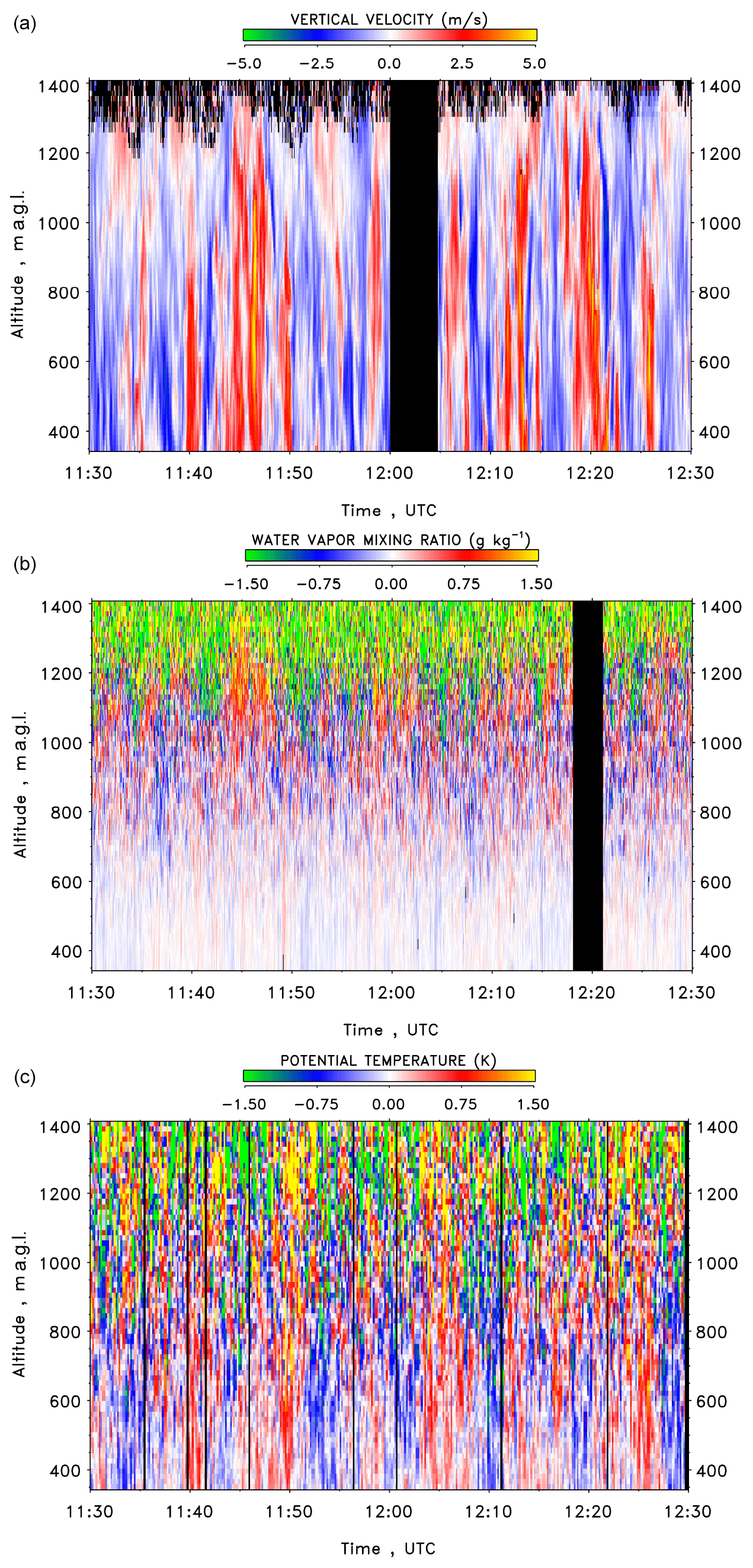
Figure 2 Time–height cross section of w^′ (a, 1 s resolution), m^′ (b, 1 s resolution), and θ^′ (c, 10 s resolution). The black areas indicate measurement gaps or data identified as outliers.

4.3 Transverse temporal autocovariance functions and spectra for vertical wind

After the determination of the ACFs of the time series, we studied their shapes for all three variables of interest.

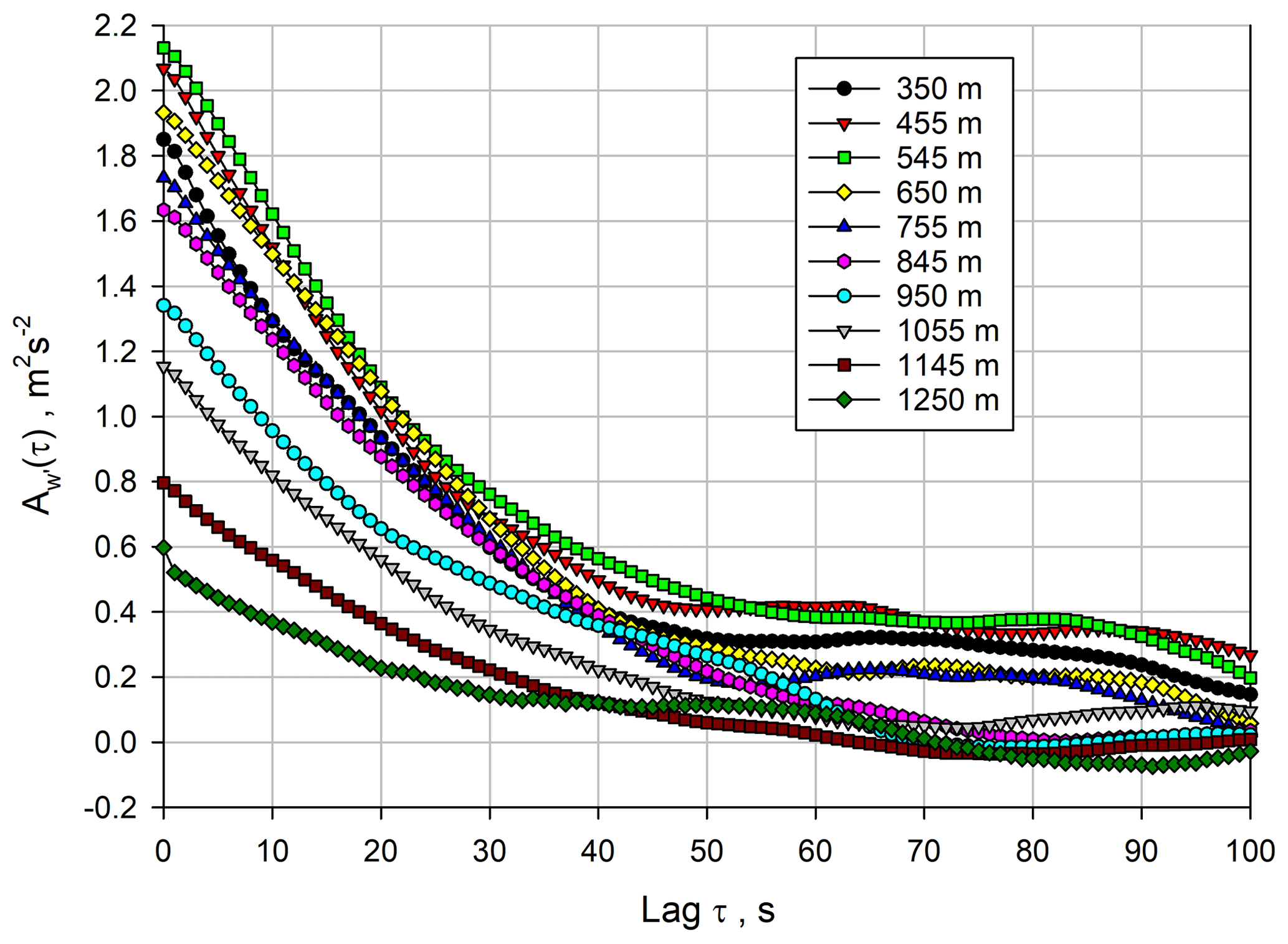
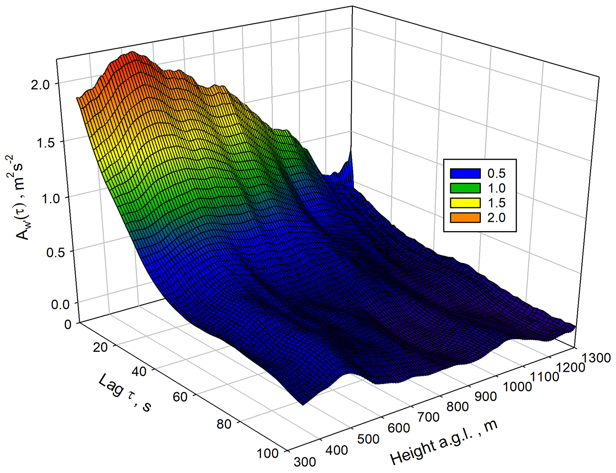
We started with the examination of $A_{w^{\prime }}\left(\mathit{\tau }\right)$ because the w^′ data provided the best resolution and SNR in the ML. The results are presented in Fig. 3 between 350 and 1250 m. The small deviations between lags 0 and 1 confirm the low noise level of the w^′ measurements. Atmospheric variance associated with mesoscale features affects the ACFs beginning at about lag 25 and beyond. This is also visible in the 3D representation of the ACFs, which is presented in Fig. 4. This figure highlights one of the advantages of the range-resolved lidar measurements because mesoscale influences on the ACFs can be studied as a function of height. It seems that there is more micro- to mesoscale influence at heights between 400–600 m, which may be related to wind shear in the horizontal wind profile at the same height range. However, as these features do not influence the ACFs at small lags, a suitable range of lags can be chosen for the fit of the ACF coefficients in the inertial subrange.

Figure 3 $A_{w^{\prime }}\left(\mathit{\tau }\right)$ for a variety of heights using the 1 s data and applying Eq. (5).

Figure 4 3D plot of $A_{w^{\prime }}(\mathit{\tau },z)$ based on the 1 s data.

The suitable ranges for the fits of the ACFs can be evaluated in more detail using Eqs. (8)–(10) or (11)–(13). The latter is visualized in Fig. 5 for a height of 545 m. For $\stackrel{\mathrm{‾}}{{w^{\prime }}^{\mathrm{2}}}$ around 2.6 m² s⁻², the result for k_w is approximately constant for a range between 7 to 25 lags. This result did not change considerably for other heights (not shown) but even extended to lag 30 at 845 m. We assume that the deviation of the ACF at small lags is due to the spatial filtering of turbulent fluctuations in each range gate of 60 m, as has already been studied by Frehlich and Cornman (2002). A minimum fit lag of 7 corresponds well with the approach of Bonin et al. (2017), who used the along-beam averaging length (60 m in our case) divided by the mean horizontal wind speed (8–9 m s⁻¹ here) as a timescale beyond which volume-averaging effects can be neglected. Up to about lag 25, no height dependence of the onset of the mesoscale variability was found so that we identified for this measurement situation an outer timescale of turbulence I_out≈25 s, limiting the inertial subrange. Therefore, a range of 7 to 25 lags was chosen for the fits of the ACFs for the 1 s data.

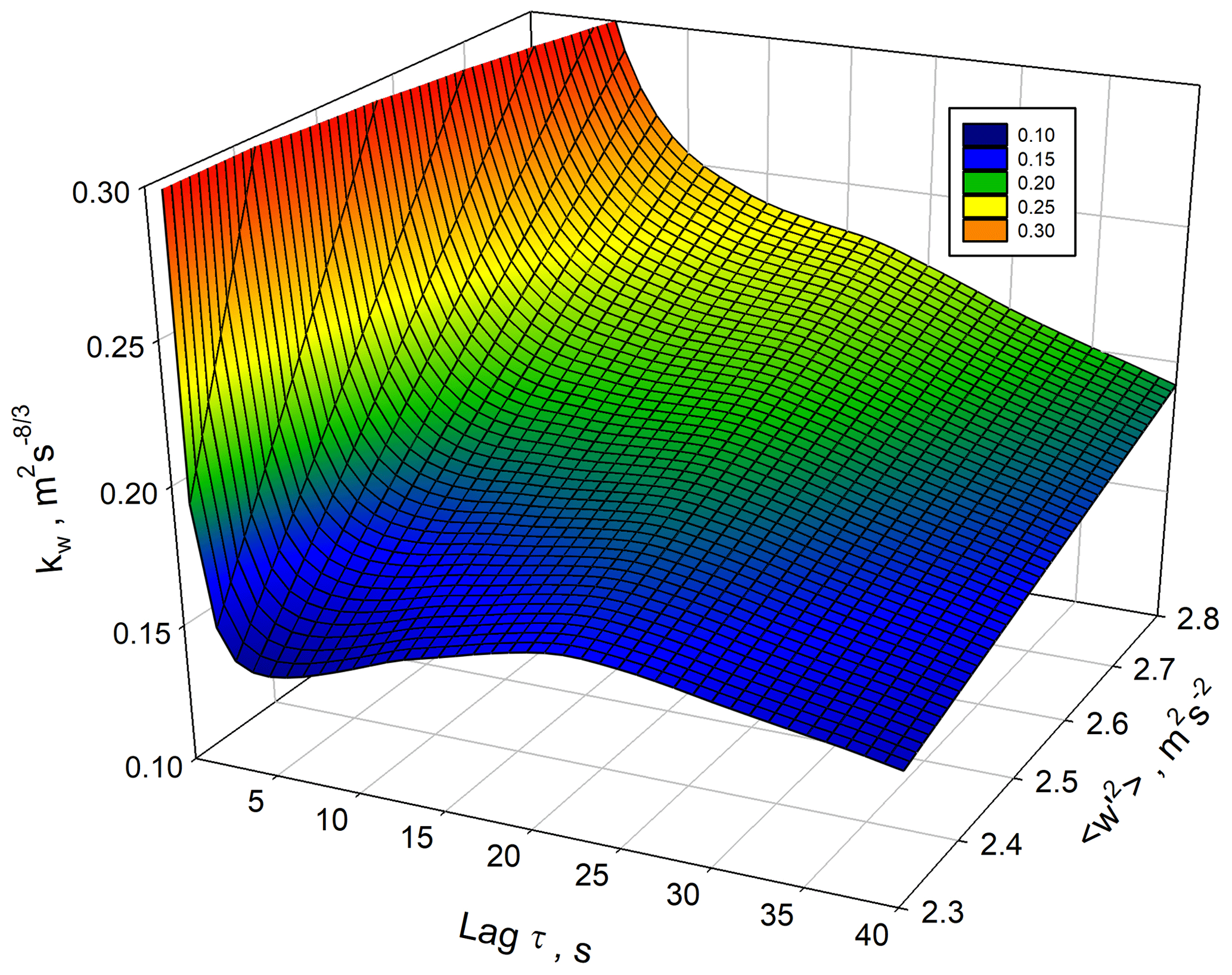
Figure 5 Example of the evaluation of the range of suitable lags according to Eq. (11) at a height of 545 m.

Figure 6 shows the corresponding series of power spectra $S_{w^{\prime }}\left(\mathit{\nu }\right)$. There is a nearly height-independent spectral maximum around 0.003 Hz and another one at 0.01 Hz. For higher frequencies, the shape of the spectra corresponds very well with the inertial subrange up to a frequency of ν_I≈0.1 Hz. This behavior is nearly height independent. Beyond this frequency, the roll off of the spectra with a steeper slope is very likely attributable to the spatial filter effects due to the single-shot pulse length. Because of the high SNR of the vertical wind data, it is very useful to perform the vertical wind analyses with a time resolution of 1 s in order to study the ACFs at small lags, which translates to the shape of the power spectra close to the Nyquist frequency of ν_N=0.5 Hz. This allows for estimating the loss of $\stackrel{\mathrm{‾}}{{w^{\prime }}^{\mathrm{2}}}$ due to the spatial filtering, which is approximately 1 % here. All these effects are consistent with and can also be detected in the temporal domain using the ACFs, as discussed above. Therefore, we recommend performing all turbulence analyses in the temporal domain (i.e., using autovariances) because the Fourier transformation does hardly provide additional information and introduces additional noise due to the transformation process.

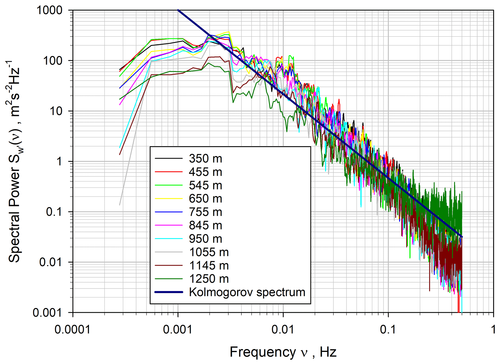
Figure 6 Power spectrum $S_{w^{\prime }}\left(\mathit{\nu }\right)$ of the vertical wind fluctuations on double-logarithmic scales for a variety of heights. The theoretical $-\mathrm{5}/\mathrm{3}$ slope of the inertial subrange is shown as a solid dark blue line.

It is essential to investigate the sensitivity of the ACFs for both 1 s and 10 s resolutions in order to find out whether the coarser time resolutions can be used as well.

Figure 7 demonstrates that the ACFs agree very well and that it is possible to use either 1 s or 10 s resolution; however, the number of lags for the fit of the ACFs has to be adapted. Except for situations where a nonlinear dependency of noise errors is reached, 1 s data analyses are preferred because in this case the resulting noise errors of the turbulence data are independent of the time resolution, but the inertial subrange is better resolved. As mentioned above, a range of 7–25 lags was used for the 1 s resolution data, corresponding to about 1–3 lags for 10 s data. The total measured variance at lag 0 was smaller for 10 s data because the atmospheric variance at scales between 1 and 10 s is not captured, and the noise variance was slightly lower because of the additional time averaging. Figure 7 also shows that the fits of the ACFs using the chosen lags of 7–25 for the 1 s data (colored solid lines) resulted in very good agreement with the measured ACFs. For instance, at 845 m, the fit provided an estimated atmospheric variance of 1.83 m² s⁻¹ and k_w≃0.11 m² s${}^{-\mathrm{8}/\mathrm{3}}$.

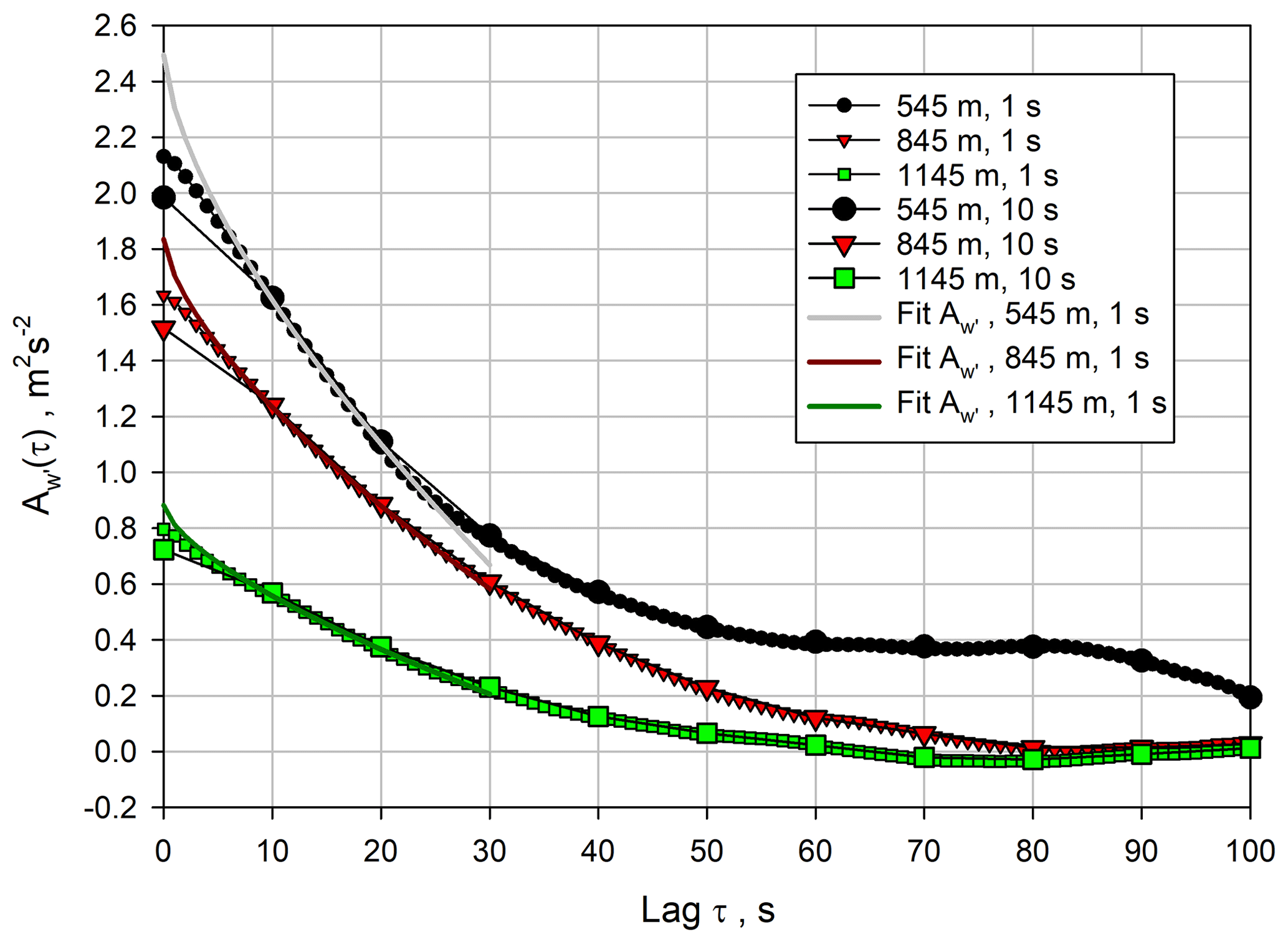
Figure 7 Comparison of $A_{w^{\prime }}$ using 1 or 10 s resolutions of the vertical wind speed data. Large symbols: 10 s resolution, smaller symbols: 1 s resolution. Colored solid lines: fits of the theoretical shapes of the ACFs using the 1 s data.

Using these lag ranges for fitting the ACFs, we determined the profiles of the integral timescale 𝒯_w and the variance of the vertical wind fluctuations for both the 1 s and the 10 s data. The results are presented in Fig. 8. The 𝒯_w profiles were derived with Eq. (17), which turned out to be most robust, and agree very well in the ML within a few seconds and amount here to 𝒯_w≃20 s. There seems to be a reduction in 𝒯_w in the IL, which is particularly strong for the 10 s results for 𝒯_w. However, it is very likely that this was due to systematic effects by the reduction in data points after quality control. The reduction was less for the 1 s 𝒯_w data where more data points were available in the IL and resulted in an estimate of 𝒯_w≃16 s in this region. These considerations show that for this type of Doppler lidar and its measurement performance, the 1 s data should be used for turbulence analyses.

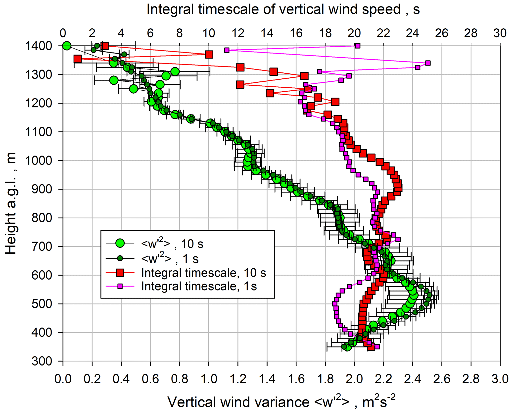
Figure 8 Small dark green and large green circles: profiles of the variance of the vertical velocity fluctuations for 1 and 10 s data, respectively, including noise error bars. Small pink and large red squares: the corresponding results for the integral timescale 𝒯_w.

A similar conclusion can be derived for the profiles of the vertical wind variance $\stackrel{\mathrm{‾}}{{w^{\prime }}^{\mathrm{2}}}$. The error bars for the variance were derived according to Wulfmeyer et al. (2016), Appendix b.4. The variance profiles agree very well, except in the lower ML where the 1 s data derive a slightly higher variance. In the IL, the 10 s data are noisier than for 𝒯_w, which we attribute again to fewer data points and resulting poorer sampling statistics. In this region, we derived a decay of the vertical wind variance, resulting in values of $\stackrel{\mathrm{‾}}{{w^{\prime }}^{\mathrm{2}}}\simeq \mathrm{0.4}$–0.6 m² s⁻². The maximum of the variance profile is located at 530 m, which corresponds to 0.4 $z/z_i$. The variance maximum is approximately 2.5 m² s⁻². This is in good agreement with previous results (Lenschow et al., 2000; Lothon et al., 2006, 2009). These results confirm that the 1 s data should be preferred for vertical wind turbulence analyses, and, therefore, we proceeded with these data for the derivation of turbulence profiles.

4.4 Transverse temporal autocovariance functions and spectra for water-vapor mixing ratio

For the mixing ratio fluctuations, we are challenged by the trade-off between the accuracy and resolution of the WVDIAL measurements. The nonlinear reduction in system noise as a function of the spatial resolutions is explained in Wulfmeyer et al. (2015, Eq. 28), whereas the reduction in noise due to temporal averaging behaves the same as for the DL for high SNR and also becomes nonlinear at low SNR, for example due to background signal subtraction. To our knowledge, the UHOH WVDIAL is currently the active remote sensing system that measures water-vapor profiles and their fluctuations with the highest resolution and accuracy (Späth et al., 2016; Behrendt et al., 2020). However, it is still necessary to find the best compromise with respect to spatial and temporal resolutions to measure the mixing ratio fluctuations. Therefore, we investigated the measurements using 1 and 10 s resolutions. However, we kept a vertical resolution of 100 m (see Sect. 4.2). At higher vertical resolution, the data became too noisy, and we wanted to avoid stronger spatial filtering effects at coarser resolution.

The ACFs are presented in Fig. 9. This figure confirms that at 1 s resolution, the measurements in the near range are not strongly influenced by noise, but the variance in the WVMR is also very small. In the ML, the mixing ratio variance increases and reaches a maximum in the IL (in contrast to the vertical wind variance), but this is also true for the system noise. Fortunately, the combination of 1 or 10 s temporal and 70 m spatial resolutions provides a compromise so that the atmospheric variance can still be recovered throughout the CBL. This is reflected in Fig. 9. Although the total variances of the time series and the contribution of the noise variances are visible in the marked increase at lag 0, it is still possible to separate noise and atmospheric variance by the extrapolation of the ACFs to lag 0.

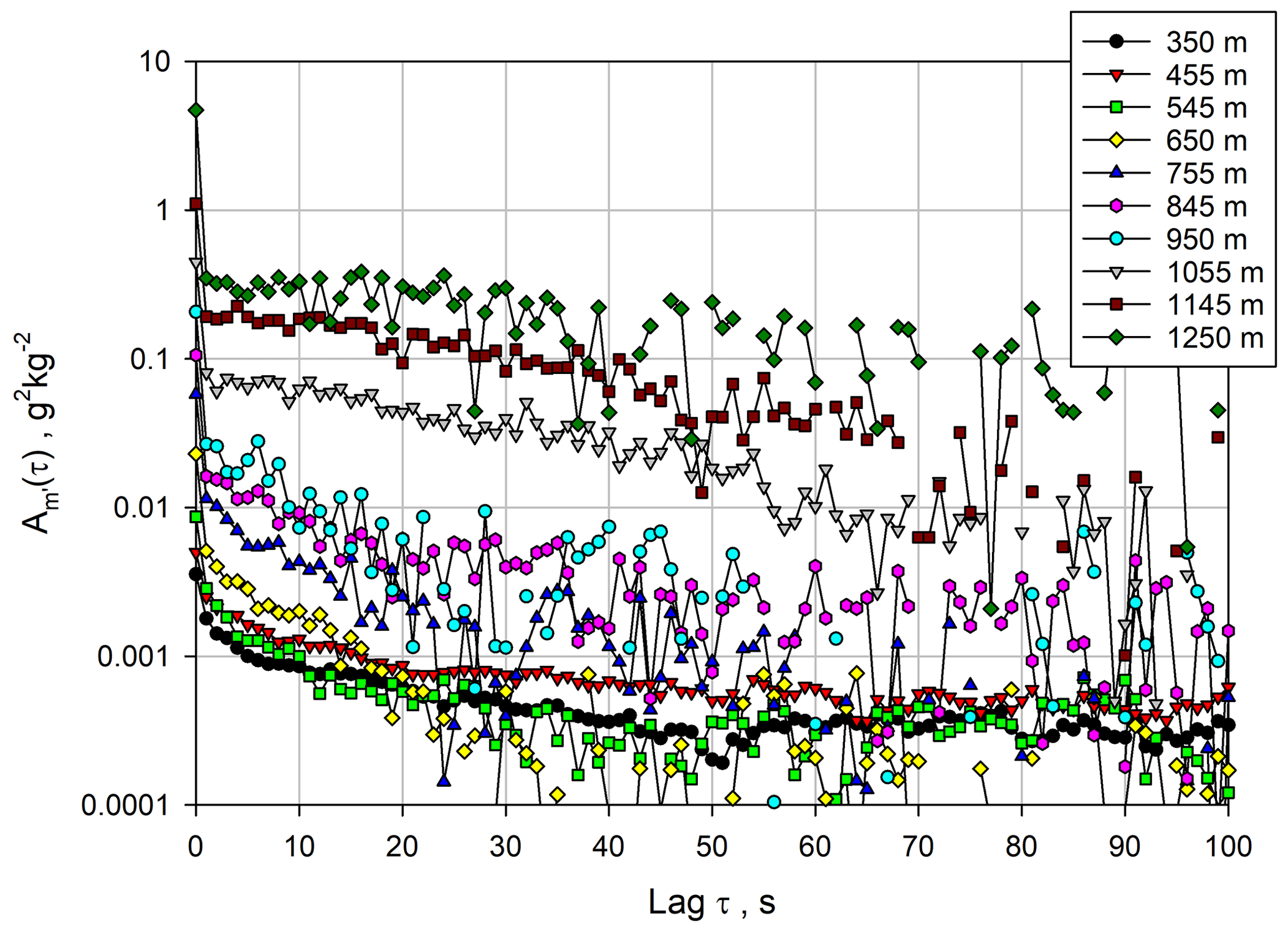
Figure 9 $A_{m^{\prime }}\left(\mathit{\tau }\right)$ for a variety of heights using Eq. (6). Note that the ACFs are shown on a logarithmic scale in order to capture the large dynamic range of the WVMR variances dependent on height.

The comparison between the ACFs computed using the 1 and 10 s resolutions is presented in Fig. 10. As for the vertical wind data, a range of 7–25 lags for the 1 s data and 1–3 lags for the 10 s data turned out to be optimal for the fit of the ACFs. The fits using the 1 s data are also shown in this plot up to lag 30 and agree well with the theoretical shapes of the ACFs. The power spectra for the 1 s data are shown in Fig. 11. There is an apparent deviation from the expected slope in the inertial subrange at high frequencies. However, these deviations are almost entirely due to the high noise levels, which led to a deviation from the $-\mathrm{5}/\mathrm{3}$-slope on the logarithmic scale. This is substantiated by the fits (solid green, dark red, and grey lines) of the spectra to the Kolmogorov function ${\mathit{\nu }}^{-\mathrm{5}/\mathrm{3}}$ (solid blue line) in the inertial subrange plus the noise floor. These fits show that the WVDIAL still resolves atmospheric fluctuations over the 0.005–0.05 Hz range, but these are masked by the larger noise floor. Therefore, in all cases, the inertial subrange is resolved but this is less obvious due to the higher noise level. This is particularly important for the critical measurements in the IL (i.e., the data in green at 1145 m) where the molecular destruction rate reaches a maximum, which at least should be quantified by this measurement method.

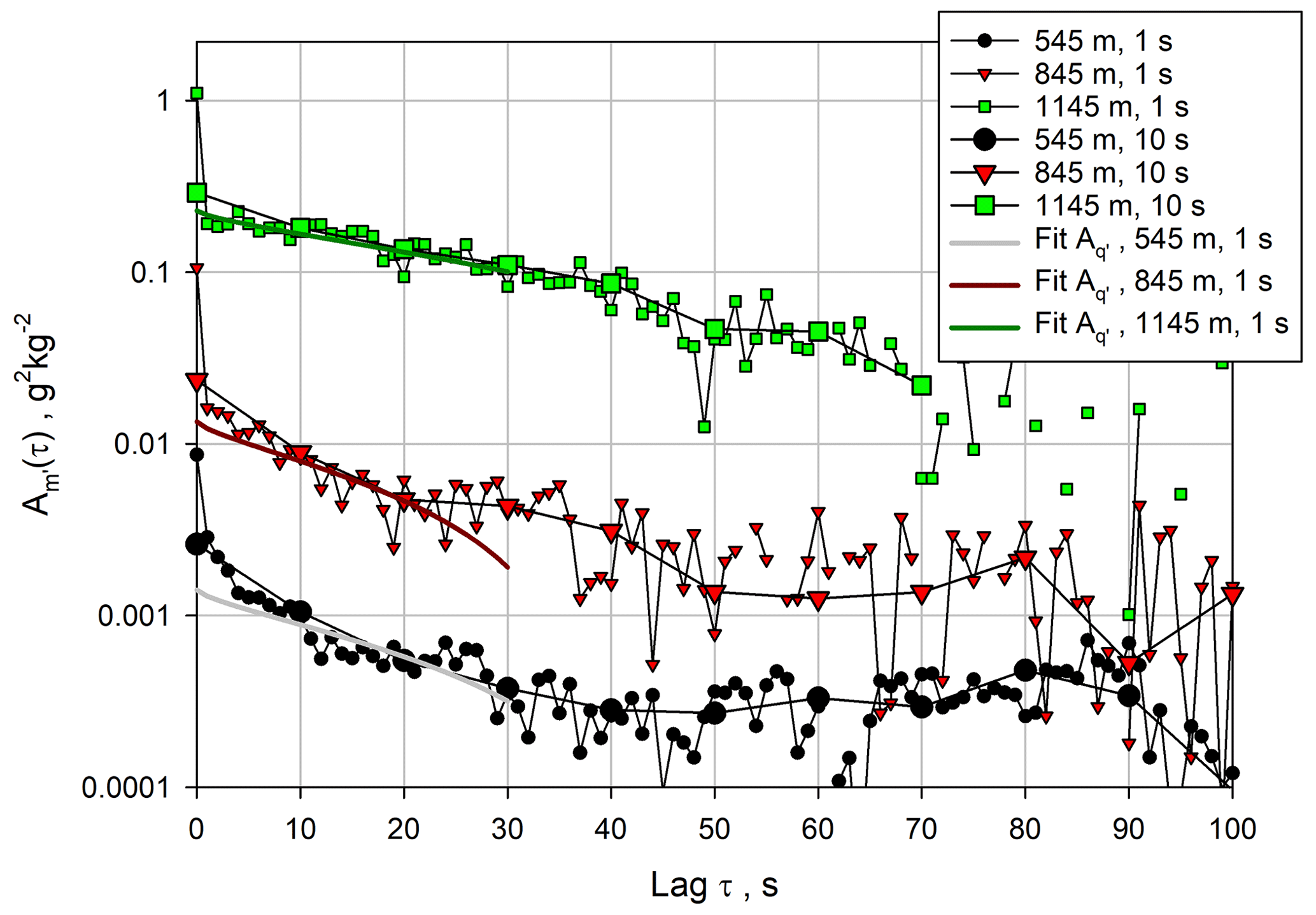
Figure 10 Comparison of $A_{m^{\prime }}\left(\mathit{\tau }\right)$ for three heights using either 1 s or 10 s data. Solid lines: fits of the theoretical shapes of the ACFs.

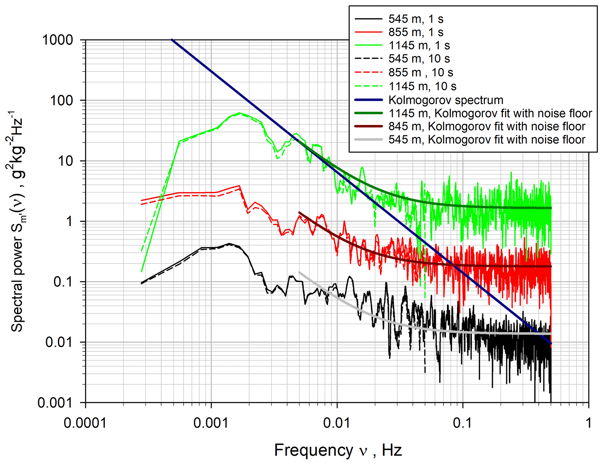
Figure 11 Power spectra of the WVMR fluctuations using 1 s data. The 10 s spectra are very consistent (not shown). The fits of the Kolmogorov spectrum with the noise floor are also shown.

Using these lag ranges for fitting the ACFs, we determined the profiles of the integral timescale 𝒯_m and the variance of the WVMR fluctuation $\stackrel{\mathrm{‾}}{{m^{\prime }}^{\mathrm{2}}}$ for both the 1 s and the 10 s data. Again, the error bars for the variance were derived according to Wulfmeyer et al. (2016, Appendix b.4). The results are presented in Fig. 12. Both data sets are plotted on a log scale to visualize the strong nonlinear increase in $\stackrel{\mathrm{‾}}{{m^{\prime }}^{\mathrm{2}}}$ in the ML and the capability of the WVDIAL to recover this large dynamic range of atmospheric variances. In the ML, the determination of 𝒯_m is strongly influenced by system noise at low variance values because in this case k_m is also small, resulting in a large uncertainty in 𝒯_m (see Eq. 17). Nevertheless, the 1 and 10 s are consistent within a few seconds. On average in the ML is 𝒯_m≃20 s similar to the 𝒯_w of the vertical wind. However, in the IL, the 10 s 𝒯_m increases significantly to around 50 s, whereas the 1 s 𝒯_m also shows strong fluctuations to very small values. Here, we consider the 10 s data to be more realistic because the noise level of the 1 s data increases in a nonlinear manner above the CBL so that it is better to use longer time averages.

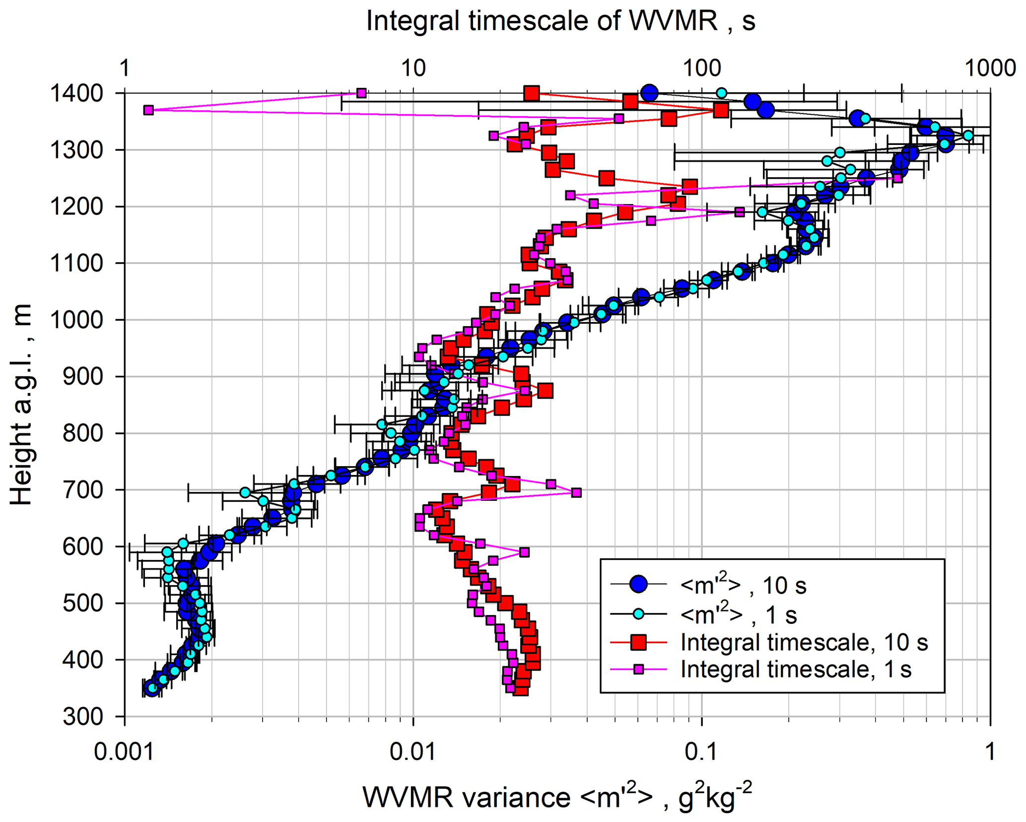
Figure 12 Small cyan and large blue circles: profiles of the variance of the WVMR fluctuations for 1 and 10 s data, respectively. Small pink and large red squares: the corresponding results for the integral timescale 𝒯_m. The vertical variability in 𝒯_m is likely due to the division by small and noisy values of k_m (see Eq. 17).

The profiles of $\stackrel{\mathrm{‾}}{{m^{\prime }}^{\mathrm{2}}}$ using 1 or 10 s data are very consistent in the entire CBL, confirming our methodological approach to determine $\stackrel{\mathrm{‾}}{{m^{\prime }}^{\mathrm{2}}}$ using different time resolutions. Using the extrapolation of the ACF to lag 0, reasonable estimates of $\stackrel{\mathrm{‾}}{{m^{\prime }}^{\mathrm{2}}}$ are derived even if the inertial subranges are not fully resolved. Also, over the entire CBL, there is almost no evidence of loss of variance due to temporal filtering effects. With the WVDIAL, it is possible to derive $\stackrel{\mathrm{‾}}{{m^{\prime }}^{\mathrm{2}}}$ and its nonlinear increase over nearly 3 orders of magnitude in the ML. In the IL, $\stackrel{\mathrm{‾}}{{m^{\prime }}^{\mathrm{2}}}$ reached a maximum very close to z_i. Interestingly, we found two maxima in the $\stackrel{\mathrm{‾}}{{m^{\prime }}^{\mathrm{2}}}$ profile, one at 1150  with a value of $\stackrel{\mathrm{‾}}{{m^{\prime }}^{\mathrm{2}}}\simeq \mathrm{0.25}$ g² kg⁻² and the other one at z_i with a value of $\stackrel{\mathrm{‾}}{{m^{\prime }}^{\mathrm{2}}}\simeq \mathrm{0.75}$ g² kg⁻². In the following, we used the 1 and 10 s k_w profiles in combination with the 10 s k_m profiles because the latter provided more robust results in the IL.

4.5 Transverse temporal autocovariance functions and spectra for potential temperature

For the potential temperature fluctuations, it is particularly difficult to derive structures in the ACF and the power spectra due to the large noise level in the TRRL observations. Although the improvement of TRRL towards the resolution of temperature fluctuations was substantial in recent years (see, e.g., Lange et al., 2019), it is still only possible to study the data with 10 s resolution. Nevertheless, the WVDIAL data analyses demonstrated that based on a careful choice of range bins for the fits, it did not make a large difference to use either 1 or 10 s for the determination of variance and temporal integral scale profiles. Therefore, we also applied this technique to the 10 s TRRL data to provide realistic profiles of 𝒯_θ, $\stackrel{\mathrm{‾}}{{{\mathit{\theta }}^{\prime }}^{\mathrm{2}}}$, and k_θ.

The corresponding ACFs are presented in Fig. 13, and the fits to the theoretical shapes of the ACFs for three heights are shown in Fig. 14. Over all ranges, the derivation of the atmospheric temperature variance and the slope of the ACFs are at the detection limits. This is also visible in the power spectrum in Fig. 15. A range that corresponds to the inertial subrange is barely visible. However, this is also not necessary, as long as the 10 s data contain the major contributions of $\stackrel{\mathrm{‾}}{{{\mathit{\theta }}^{\prime }}^{\mathrm{2}}}$, as shown for the WVDIAL data.

Figure 13 $A_{{\mathit{\theta }}^{\prime }}\left(\mathit{\tau }\right)$ for a variety of heights using Eq. (7) at a resolution of 10 s.

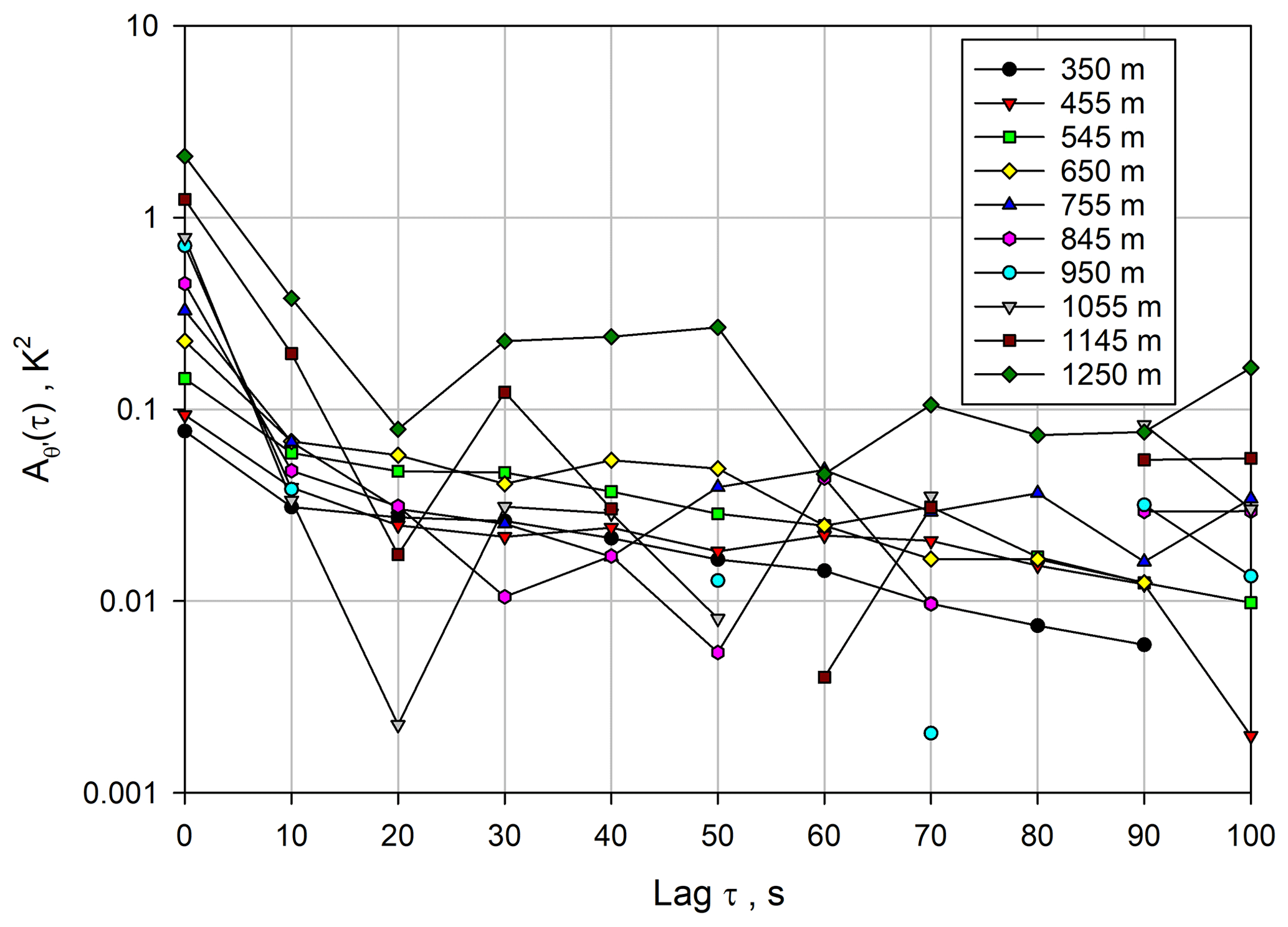
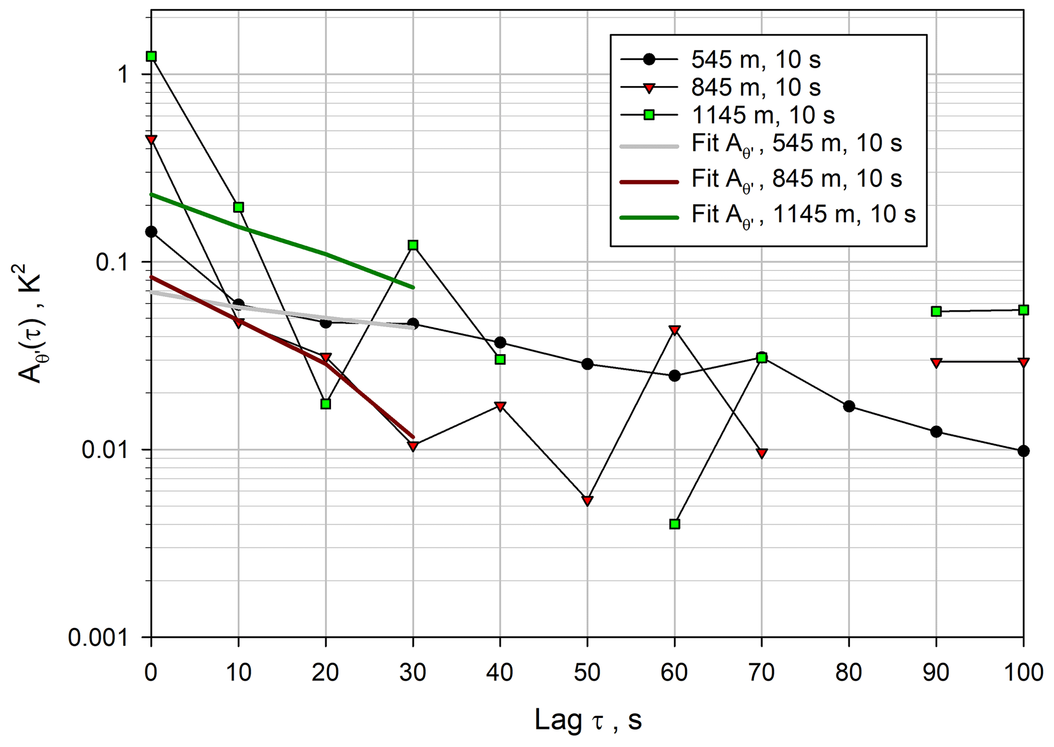
Figure 14 $A_{{\mathit{\theta }}^{\prime }}\left(\mathit{\tau }\right)$ for 10 s at three heights with the corresponding fits of the theoretical shape of the ACFs.

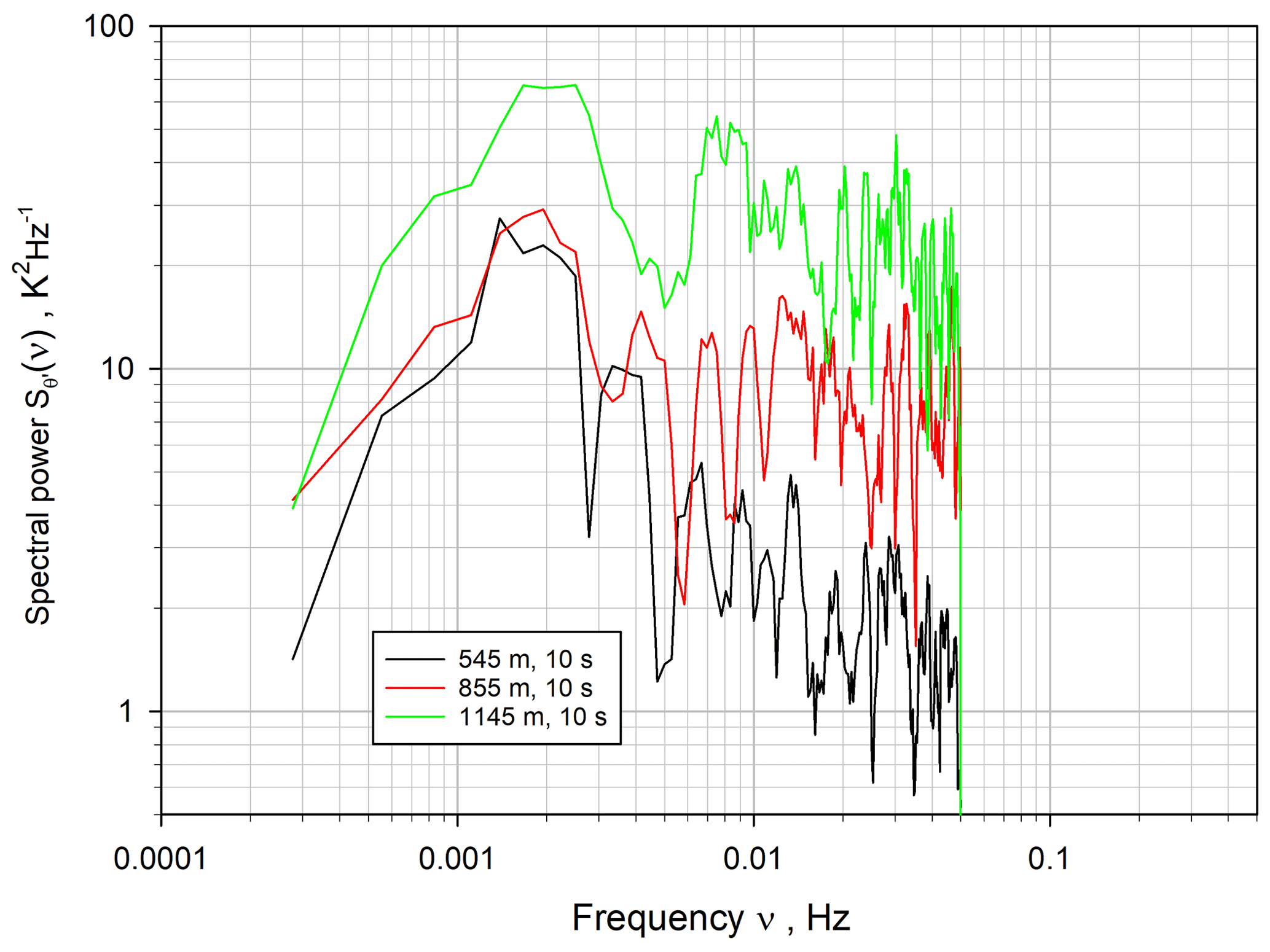
Figure 15 Power spectrum $S_{{\mathit{\theta }}^{\prime }}\left(\mathit{\nu }\right)$ of the potential temperature fluctuations on double-logarithmic scales for a variety of heights. The theoretical $-\mathrm{5}/\mathrm{3}$ slope of the spectra is hardly visible due to the high noise level of the data and the need to use 10 s data. However, a large part of the atmospheric variances is still recovered over this spectral range.

Using lags 1–3 for fitting the ACFs, we determined the profiles of the integral timescale 𝒯_θ and the variance of the potential temperature fluctuations. As above, the error bars for the variance were derived according to Wulfmeyer et al. (2016, Appendix b.4). The results are presented in Fig. 16. For the same reasons as for 𝒯_m, 𝒯_θ is strongly affected by system noise at low variance values. In spite of the large fluctuations, 𝒯_θ seems to be larger than 𝒯_w and 𝒯_m in the lower ML. Our estimate of 𝒯_θ ranges between ≃30 s in the ML and ≃14 s in the IL. In contrast to 𝒯_m, there seems to be a reduction in 𝒯_θ from the ML towards the IL. In the majority of the ML, all 𝒯 values for w^′, m^′, and θ^′ are similar for the 1 and 10 s data and range between ≃20–30 s.

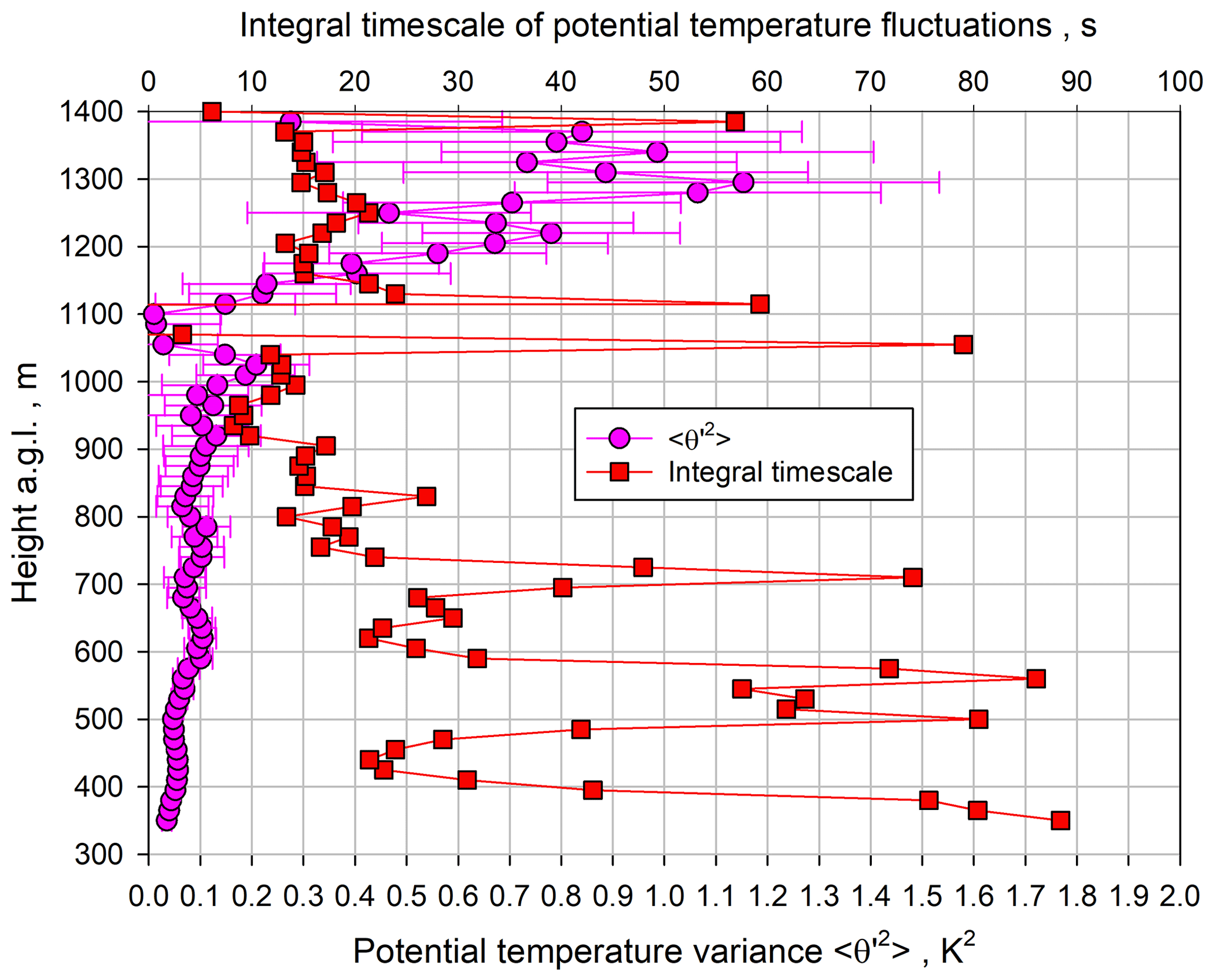
Figure 16 Pink circles: profiles of the variance of the potential temperature fluctuations for 10 s data. Red squares: the corresponding results for the integral timescale.

Using the fits of the ACFs, we are able to detect the expected small $\stackrel{\mathrm{‾}}{{{\mathit{\theta }}^{\prime }}^{\mathrm{2}}}$ in the ML and its increase to a maximum in the IL, reaching a statistically significant $\stackrel{\mathrm{‾}}{{{\mathit{\theta }}^{\prime }}^{\mathrm{2}}}\simeq \mathrm{1.1}$ K² very close to z_i. In contrast to $\stackrel{\mathrm{‾}}{{m^{\prime }}^{\mathrm{2}}}$, we did not find a strong nonlinear increase in $\stackrel{\mathrm{‾}}{{{\mathit{\theta }}^{\prime }}^{\mathrm{2}}}$ in the ML, but it remained around ≃0.1 K² over almost the entire part of the ML. As for the $\stackrel{\mathrm{‾}}{{m^{\prime }}^{\mathrm{2}}}$ profile, there seems to be another slight peak in the variance at 1020 m, which corresponds to approximately 0.8 $z/z_i$ with a value of $\stackrel{\mathrm{‾}}{{{\mathit{\theta }}^{\prime }}^{\mathrm{2}}}\simeq \mathrm{0.2}$ K².

A comparison of the integral length scales is presented in Fig. 17. There are strong deviations in the lower ML and the IL; however, in the center of the ML, the integral length scales are similar and amount to ≃160 m. As for m^′, we applied the 1 and 10 s k_w profiles in combination with the 10 s k_θ profiles because only the latter provided robust results in the CBL.

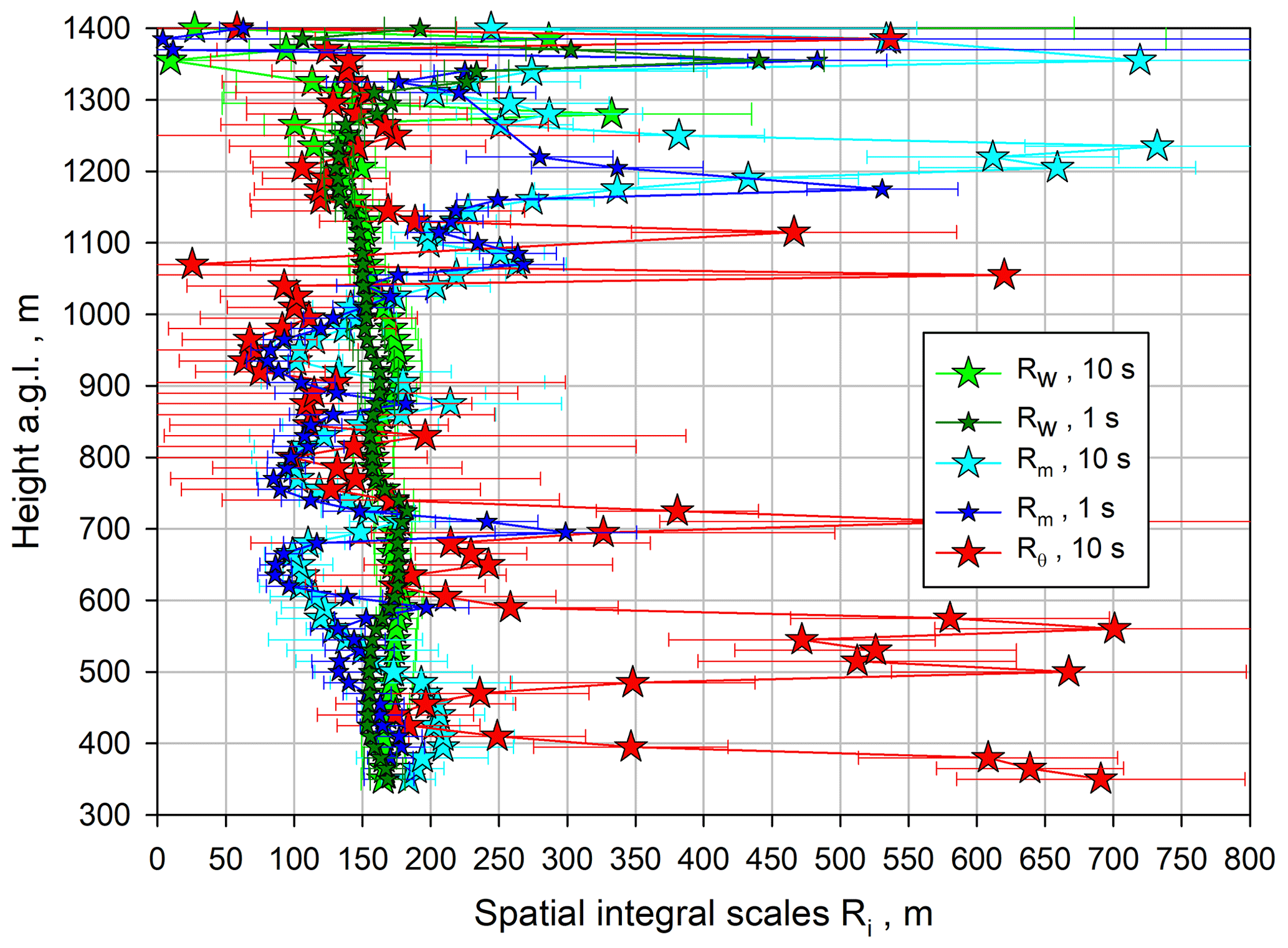
Figure 17 Comparison of the integral length scales ℛ_w (small dark green and large green stars), ℛ_m (small blue and large cyan stars), and ℛ_θ (red stars), including error bars due to noise error propagation according to Wulfmeyer et al. (2016, Appendix b.4), adapted to ℛ_i.

5 Profiles of TKE dissipation and molecular destruction rates

5.1 TKE dissipation

The derivation of the profiles of the ACF coefficient k_w and the TKE dissipation ϵ (see Eq. 18) using the 1 and 10 s data is presented in Fig. 18. The error bars are based on Wulfmeyer et al. (2016, Appendix b.4). Similar to $\stackrel{\mathrm{‾}}{{w^{\prime }}^{\mathrm{2}}}$, both k_w and ϵ reach a maximum near 530 m, which corresponds to approximately 0.4 $z/z_i$. Up to this height, likely due to filter and noise effects, the difference between the 1 and 10 s data is the largest, whereas the results are very similar in the rest of the ML. At the maximum, $\mathit{ϵ}\simeq \mathrm{1}\times {\mathrm{10}}^{-\mathrm{2}}$ m² s⁻³ for the 1 s data and $\mathit{ϵ}\simeq \mathrm{8.5}\times {\mathrm{10}}^{-\mathrm{3}}$ m² s⁻³ for the 10 s data. At this height, k_w≃0.19 m² s${}^{-\mathrm{8}/\mathrm{3}}$ for the 1 s data and k_w≃0.17 m² s${}^{-\mathrm{8}/\mathrm{3}}$ for the 10 s data. Both ϵ and k_w decrease towards the IL to values of around $\simeq \mathrm{1}\times {\mathrm{10}}^{-\mathrm{3}}$ m² s⁻³ and ≃0.04 m² s${}^{-\mathrm{8}/\mathrm{3}}$ at 1300 m, respectively. In the IL, as expected from the analyses of the variances and the integral timescales, the 10 s data showed a high variability, whereas the 1 s data still permitted robust derivations of ϵ and k_w. As also in the ML a more accurate determination of turbulence profiles can be expected due to the better resolution of the inertial subrange, we used the 1 s profiles for the derivations of molecular destruction rates below.

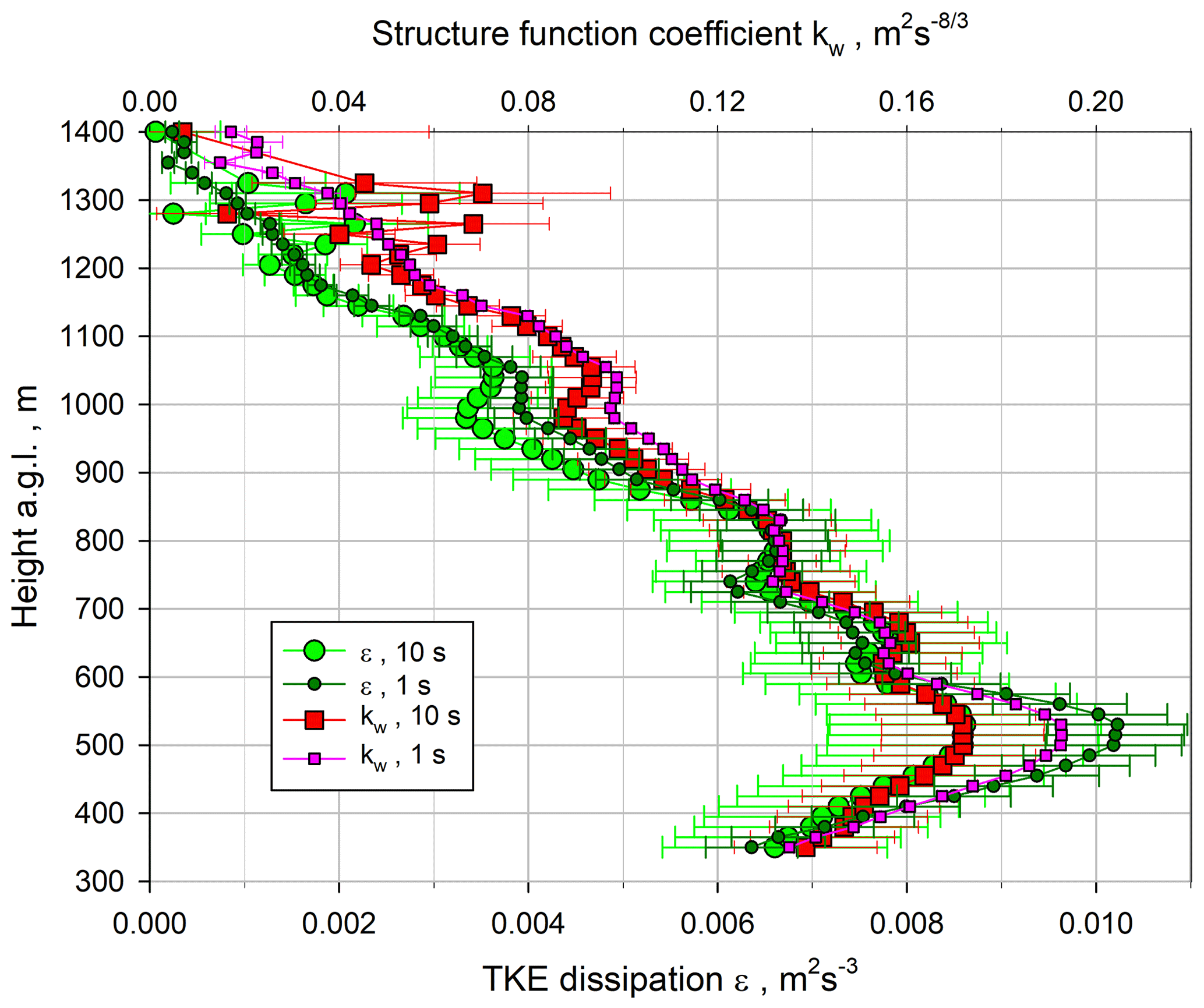
Figure 18 Small dark green and large light green circles: profiles of TKE dissipation ϵ using Eq. (18) derived with 1 and 10 s resolutions, respectively. Small pink and large red squares: corresponding profiles of the ACF coefficient k_w with 1 and 10 s resolutions, respectively.

For parameterizations of ϵ, it can be related to the vertical wind variance profile $\stackrel{\mathrm{‾}}{{w^{\prime }}^{\mathrm{2}}}$. The results are presented in Fig. 19 with the theoretical function from Eq. (19). For this fit we used all the data and inserted a mean integral length scale averaged over all data and the entire CBL, which resulted in ℛ_w≃162.5 m (see Fig. 17). Note that the averages of ℛ_w were quite consistent between the 1 s (≃ 160 m) and 10 s data (≃ 165 m) and decreased only by 20 s towards the IL so that it was valid to use just an average value for ℛ_w. Thus, we achieved

$$\begin{array}{}\text{(25)}& \mathit{ϵ}\simeq {\displaystyle \frac{\mathrm{2}}{\mathrm{5}}}{\displaystyle \frac{\mathrm{1}}{\mathrm{160}\mathrm{m}}}{\left(\stackrel{\mathrm{‾}}{{w^{\prime }}^{\mathrm{2}}}\right)}^{\mathrm{3}/\mathrm{2}},\end{array}$$

which turned out to be in excellent agreement with our measurements.

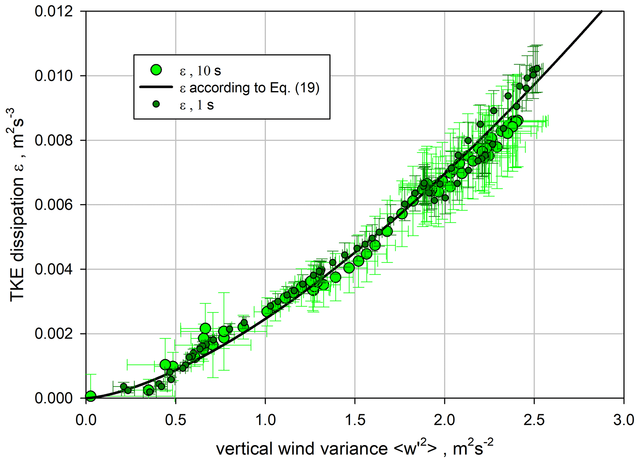
Figure 19 Small dark green circles: TKE dissipation ϵ derived with 1 s resolution. Large light green circles: ϵ derived with 10 s resolution. Solid black line: fit using Eq. (19) combining all data and using a mean spatial integral length scale ℛ_w≃162.5 m.

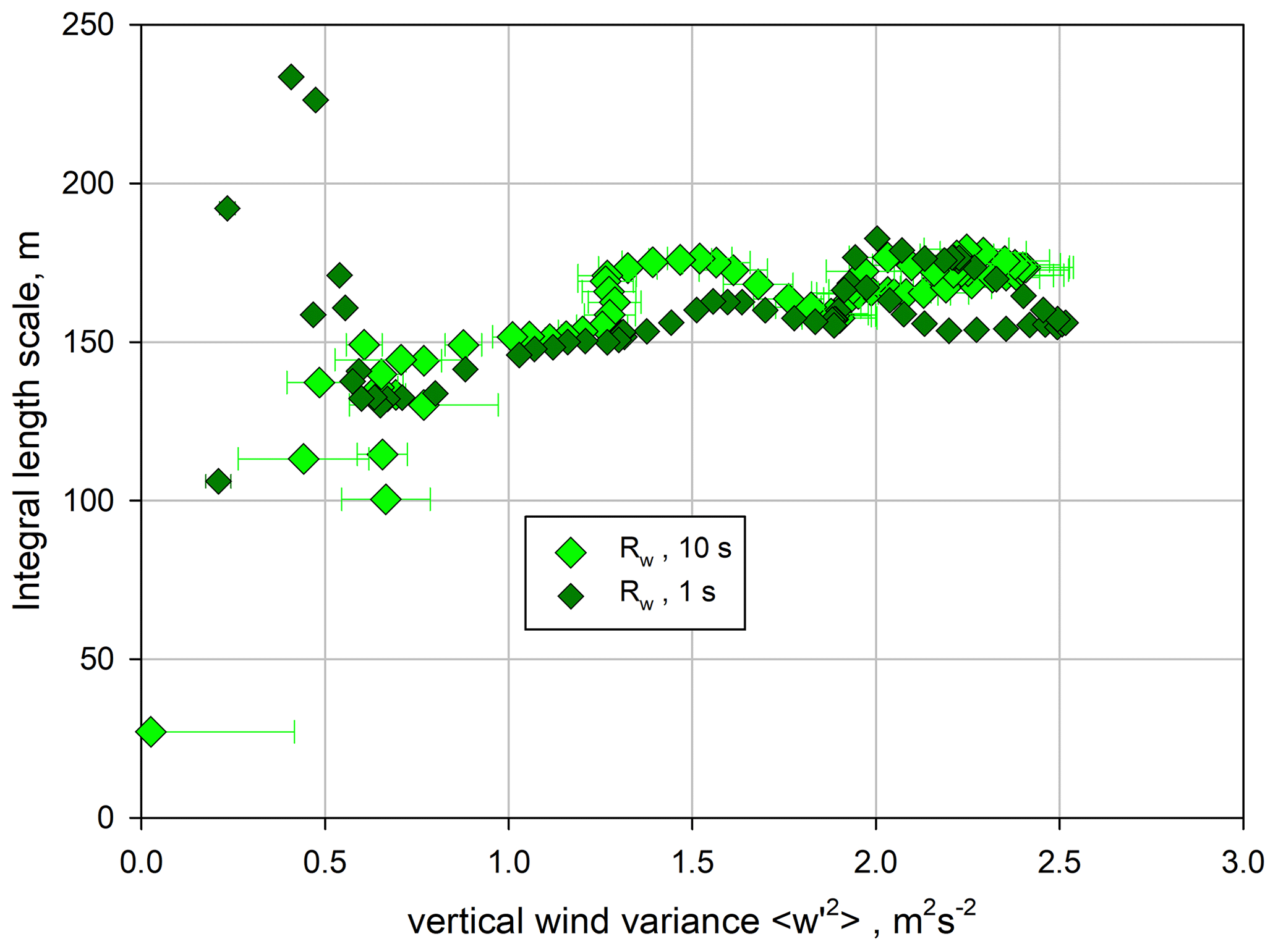
Further refinements are possible using the observed dependence of ℛ_w on $\stackrel{\mathrm{‾}}{{w^{\prime }}^{\mathrm{2}}}$, which is presented in Fig. 20. For $\stackrel{\mathrm{‾}}{{w^{\prime }}^{\mathrm{2}}}>\mathrm{0.5}$ m s⁻¹, ℛ_w seems to be fairly constant, but it is uncertain in the IL. It is important to study whether our results for ℛ_w and its small height dependence are universal so that these can also be applied to other measurements or whether it is necessary to investigate more detailed similarity relationships for ℛ_w in order to derive a more general parameterization of ϵ.

Figure 20 Dark green diamonds: ℛ_w for 1 s data. Light green diamonds: ℛ_w for 10 s data.

5.2 Profiles of molecular destruction rates

Using high-resolution profile observations of the water-vapor mixing ratio m and the potential temperature θ, the equivalent methodology can be applied to derive profiles of the ACF coefficient and the molecular destruction rates for these two scalars.

5.2.1 Molecular destruction of mixing ratio variance

The derivation of the profiles of the ACF coefficient k_m and the mixing ratio molecular destruction rate ϵ_m (see Eq. 20) is presented in Fig. 21. We present only the k_m profile for 10 s because it agreed very well with the 1 s profile in the ML, but the 1 s data became unstable and partly negative in the IL. For the derivation of ϵ_m, we used two options, the k_w profile for either 1 s or 10 s. Both resulting profiles are included in Fig. 21. Similar to $\stackrel{\mathrm{‾}}{{m^{\prime }}^{\mathrm{2}}}$, both k_m and ϵ_m maintain the double-peak structure in the CBL and reach a maximum in the IL very close to z_i. At the maximum, k_m≃0.05 g² kg⁻² s${}^{-\mathrm{2}/\mathrm{3}}$ and ${\mathit{ϵ}}_m\simeq \mathrm{7}\times {\mathrm{10}}^{-\mathrm{4}}$ g² kg⁻² s⁻¹ considering the more robust results from k_w using the 1 s data.

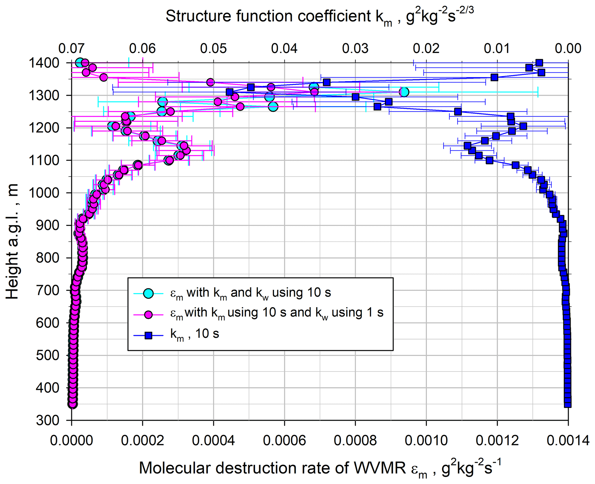
Figure 21 Small pink and large cyan circles: profiles of ϵ_m using Eq. (20) derived with 1 and 10 s resolutions for k_w, respectively. Large blue squares: profile of k_m with 10 s resolution.

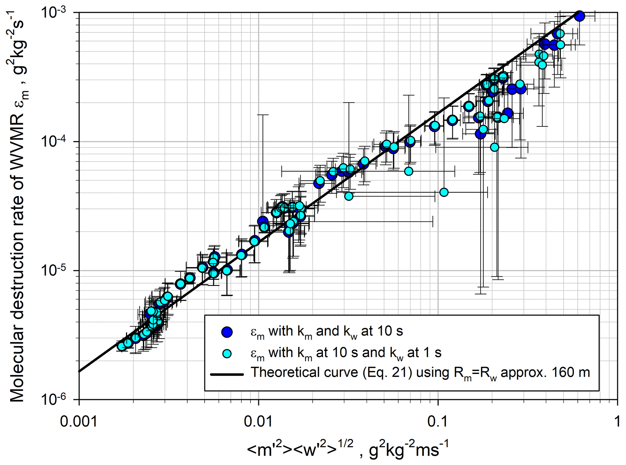
For a parameterization of ϵ_m it is very interesting to relate it to both $\stackrel{\mathrm{‾}}{{m^{\prime }}^{\mathrm{2}}}$ and $\stackrel{\mathrm{‾}}{{w^{\prime }}^{\mathrm{2}}}$ using Eq. (21). The results are presented in Fig. 22. For this comparison we used all the data and a mean integral length scale of ${\mathcal{R}}_m={\mathcal{R}}_w\simeq \mathrm{160}$ m (see also Fig. 17) and achieved

$$\begin{array}{}\text{(26)}& {\mathit{ϵ}}_m\simeq {\displaystyle \frac{\mathrm{4}}{\mathrm{15}}}{\displaystyle \frac{\mathrm{1}}{\mathrm{160}\mathrm{m}}}\stackrel{\mathrm{‾}}{{m^{\prime }}^{\mathrm{2}}}\sqrt{\stackrel{\mathrm{‾}}{{w^{\prime }}^{\mathrm{2}}}},\end{array}$$

which agrees well with our data over nearly 3 orders of magnitude. Most of the variability between theory and observation can be explained by the noise error bars. The data points of the 1 s data that deviate more from the theoretical curve (e.g., $\stackrel{\mathrm{‾}}{{m^{\prime }}^{\mathrm{2}}}\simeq \mathrm{0.1}$ g² kg⁻² and ${\mathit{ϵ}}_m\simeq \mathrm{4}\times {\mathrm{10}}^{-\mathrm{5}}$ g² kg⁻² s⁻¹) belong to the top of the IL where the derivation of ϵ_m becomes particularly uncertain. The agreement of our observations with Eq. (21) indicates that a parameterization of ϵ_m is possible with the variances $\stackrel{\mathrm{‾}}{{m^{\prime }}^{\mathrm{2}}}$ and $\stackrel{\mathrm{‾}}{{w^{\prime }}^{\mathrm{2}}}$. Obviously, this kind of plot also provides the opportunity to estimate a mean spatial integral scale between ℛ_m and ℛ_w by determining its slope.

Figure 22 Small cyan circles: ϵ_m derived with k_m at 10 s and k_w at 1 s resolutions. Large blue circles: ϵ_m derived with k_m and k_w at 10 s resolutions. Fit using Eq. (21) combining all data and using a mean spatial integral length scale of ${\mathcal{R}}_m={\mathcal{R}}_w\simeq \mathrm{160}$ m.

5.2.2 Molecular destruction of potential temperature variance

The profiles of the ACF coefficient k_θ and the potential temperature destruction rate ϵ_θ (see Eq. 22) are presented in Fig. 23. As for ϵ_m, ϵ_θ was determined using the k_w profile for either 1 s or 10 s. Similar to $\stackrel{\mathrm{‾}}{{{\mathit{\theta }}^{\prime }}^{\mathrm{2}}}$, both k_θ and ϵ_θ reach a maximum in the IL very close to z_i. At the maximum, ${\mathit{ϵ}}_{\mathit{\theta }}\simeq \mathrm{1.6}\times {\mathrm{10}}^{-\mathrm{3}}$ K² s⁻¹ and k_θ≃0.09 K² s${}^{-\mathrm{2}/\mathrm{3}}$. Here there also seems to be a second maximum below z_i at approx. 1050 m.

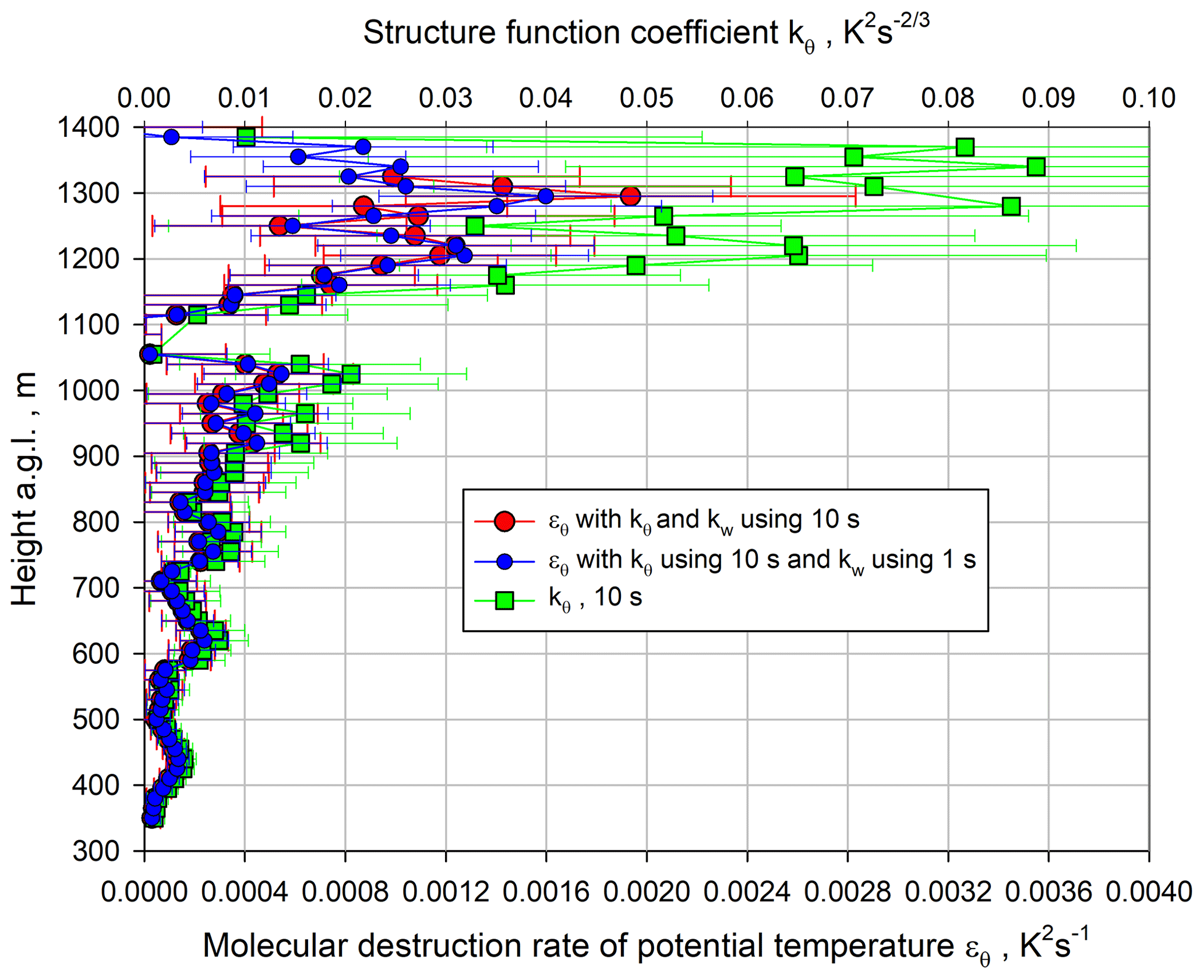
Figure 23 Small blue and large red circles: profiles of ϵ_θ using Eq. (22) derived with k_θ at 10 s resolution and k_w at 1 and 10 s resolutions, respectively. Green squares: corresponding profiles of the ACF coefficient k_θ with 10 s resolution.

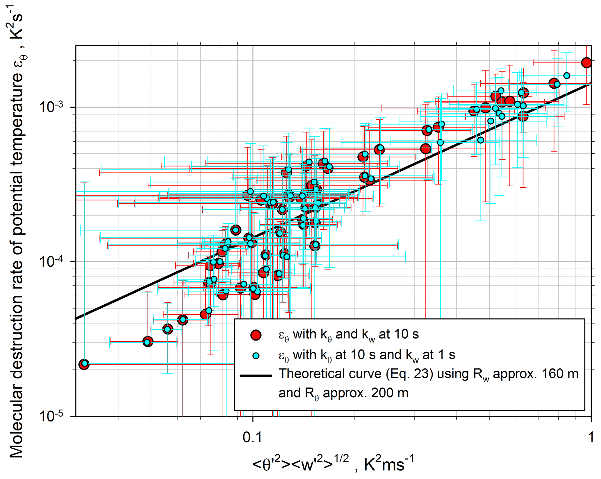
For a parameterization of ϵ_θ, we relate it to both $\stackrel{\mathrm{‾}}{{{\mathit{\theta }}^{\prime }}^{\mathrm{2}}}$ and $\sqrt{\stackrel{\mathrm{‾}}{{w^{\prime }}^{\mathrm{2}}}}$ (see Eq. 23). The results are presented in Fig. 24 with the theoretical function from Eq. (23). For this fit we used all the data and approximated the spatial integral scales in the CBL by ℛ_w≃160 m and ℛ_θ≃200 m. Thus, we estimated

$$\begin{array}{}\text{(27)}& \begin{array}{rl}{\mathit{ϵ}}_{\mathit{\theta }}& \simeq {\displaystyle \frac{\mathrm{4}}{\mathrm{15}}}{\displaystyle \frac{\mathrm{1}}{\left(\mathrm{160}\mathrm{m}{)}^{\mathrm{1}/\mathrm{3}}\right(\mathrm{200}\mathrm{m}{)}^{\mathrm{2}/\mathrm{3}}}}\stackrel{\mathrm{‾}}{{{\mathit{\theta }}^{\prime }}^{\mathrm{2}}}\sqrt{\stackrel{\mathrm{‾}}{{w^{\prime }}^{\mathrm{2}}}}\\ & \simeq {\displaystyle \frac{\mathrm{4}}{\mathrm{15}}}{\displaystyle \frac{\mathrm{1}}{\mathrm{186}\mathrm{m}}}\stackrel{\mathrm{‾}}{{{\mathit{\theta }}^{\prime }}^{\mathrm{2}}}\sqrt{\stackrel{\mathrm{‾}}{{w^{\prime }}^{\mathrm{2}}}},\end{array}\end{array}$$

which agrees reasonably well with our data. Almost all deviations between the theoretical curve and the observations can be explained by the large noise error bars.

Figure 24 Small cyan circles: ϵ_θ derived with k_θ at 10 s and k_w at 1 s resolutions. Large red circles: ϵ_θ derived with k_θ and k_w at 10 s resolutions. Solid black line: fit using Eq. (23) combining all data and using mean spatial integral length scales of ℛ_w≃160 m and ℛ_θ≃200 m.

6 Discussion

In this work, we used high-resolution time series of w^′, m^′, and θ^′ for profiling integral scales; variances; and ϵ, ϵ_m, and ϵ_θ in the CBL. We developed a technique to identify the suitable range of lags for fitting the theoretical shape of the ACFs to the data in order to consider the effects of temporal–spatial averaging/filtering using 1 or 10 s data on the resulting profiles of turbulent quantities. We did not correct our measurements further with respect to filtering effects, as the corresponding loss is generally not larger than 10 %–15 %, as demonstrated and elaborated in Lothon et al. (2006, 2009). We applied all our derivations in the temporal and spatial spaces because this handling of the data using the theoretical shape of the transversal ACF is equivalent to spectral analyses so that we avoid additional processing steps. We also calculated spectra to study the consistency and plausibility of our temporal statistics.

According to its definition, 𝒯_i is a kind of average for the typical duration of a coherent fluctuation in the inertial subrange or a way to characterize the corresponding horizontal size of a turbulent eddy according to ℛ_i≃V 𝒯_i. This assumes that the Taylor hypothesis is applicable to these scales. Lothon et al. (2006) demonstrated that a length scale L or an outer scale of turbulence can be defined where the inertial subrange becomes visible in the data, which resulted in L_i≈2.7 ℛ_i. However, this concept only works if the inertial subrange is not overwhelmed by mesoscale and microscale circulations so that its onset in the power spectra is highly variable. Related to these effects, it is essential to separate turbulent fluctuations from micro- and mesoscale fluctuations in order to determine 𝒯_i correctly. The approximation to integrate the measured ACF to its first zero crossing is not the best approach and leads to an overestimation of 𝒯_i and ℛ_i (compare, e.g., the measured and fitted ACFs in Fig. 7 at 545 m). It is fundamental to determine the range of the suitable lags first, derive k_i from this, and then use Eq. (17) to derive 𝒯_i (Wulfmeyer et al., 2016). Equation (17) provided rather robust results even at small variances and large noise levels (see Figs. 8, 12, and 16). For this procedure, it is not necessary to use a temporal resolution Δt of the data to “resolve” the inertial subrange, but it is required that a reasonable range of samples is present to realize an accurate fit of the data to the theoretical shape of the ACF. As the zero crossing τ_0,i of the extrapolated ACF is $\mathrm{5}/\mathrm{2}{\mathcal{T}}_i$ (Wulfmeyer et al., 2016), $\mathrm{\Delta }t\ll {\mathit{\tau }}_{\mathrm{0},i}$. This was the case for the 1 and 10 s data here because we found ${\mathit{\tau }}_{\mathrm{0},i}\simeq \mathrm{5}/\mathrm{2}{\mathcal{T}}_i\simeq \mathrm{50}$ s > 10 s. This explains the good agreement of the profiles of temporal and spatial integral scales, the variances, the TKE dissipation, and the molecular destruction rates for both 1 s and 10 s resolutions. Thus, we could also estimate L_i with τ_0,i or 𝒯_i because obviously $L_i\approx \mathrm{2.5}{\mathcal{R}}_i\simeq \mathrm{2.5}V{\mathcal{T}}_i\simeq V{\mathit{\tau }}_{\mathrm{0}}$.

We determined 𝒯_w≃20 s in the ML, which corresponds to ${\mathcal{R}}_w\simeq \mathrm{160}\mathrm{m}\simeq \mathrm{0.13}{z}_i$ (see Fig. 17), with an indication of a slight decrease towards the IL. Previous measurements of 𝒯_w and ℛ_w were reported in Lenschow et al. (2000) and Lothon et al. (2006). In the case studied in Lenschow et al. (2000), 𝒯_w≃60 s, resulting in ${\mathcal{R}}_w\simeq \mathrm{180}\mathrm{m}\simeq \mathrm{0.12}{z}_i$ with a slight increase towards the IL. In spite of this agreement, we need to evaluate more data consistently because Lenschow et al. (2000) used a linear fit to the ACF to derive 𝒯_w and $\stackrel{\mathrm{‾}}{{w^{\prime }}^{\mathrm{2}}}$, which could have led to an overestimation of 𝒯_w and an underestimation of $\stackrel{\mathrm{‾}}{{w^{\prime }}^{\mathrm{2}}}$. In Lothon et al. (2006) and Lenschow et al. (2012), a number of cases were analyzed, but here an integration of the ACF to the first zero crossing was used, likely leading to an even more severe overestimation of 𝒯_w. This can be the reason that Lothon et al. (2006) and Lenschow et al. (2012) found ℛ_w≃0.3 z_i, whereas we found ℛ_w≃0.13 z_i, which is a significant reduction. In any case, for future operational analyses of turbulence data, it seems to be safe to estimate the upper limit of the number of suitable lags (lag_max) for fitting the ACF with its theoretical shape in the inertial subrange according to ${\mathrm{lag}}_{max}<\mathrm{2}{\mathcal{T}}_w/\mathrm{\Delta }t\simeq \mathrm{0.25}{z}_i/\left(V\mathrm{\Delta }t\right)<{\mathit{\tau }}_{\mathrm{0},w}/\mathrm{\Delta }t$. It is necessary to substantiate this relationship with large data sets from observatories such as LAFO (Späth et al., 2023).

With respect to 𝒯_m, some results were presented in Lenschow et al. (2000), Wulfmeyer et al. (2016), and Osman et al. (2018). While we derived ${\mathcal{T}}_m\simeq \mathrm{15}\mathrm{s}\le {\mathcal{T}}_w$ in the ML with a tendency to increase towards the IL, 𝒯_m≃50–100 s was derived in these publications with a tendency to decrease towards the IL. It is essential to collect more data in combination with consistent data processing as introduced in this work to gain further insight into the statistics of 𝒯_m because, similarly to the discussion of 𝒯_w, different integration schemes and numbers of lags were used, likely resulting in an overestimation of 𝒯_m. To the best of our knowledge, 𝒯_θ has only been studied in our work as well as in Behrendt et al. (2015), Wulfmeyer et al. (2016), and Behrendt et al. (2020) using data from the same campaign but using a different number of lags, which explains why we specified a smaller 𝒯_θ≃20 s. The tendency of an increase in 𝒯_θ towards the lower ML needs more investigation in the future.

Our profile of vertical velocity variance reaches a maximum at ≃0.4 z_i with a value of $\stackrel{\mathrm{‾}}{{w^{\prime }}^{\mathrm{2}}}\simeq \mathrm{2.5}$ m² s⁻² and decreases to ≃0.2 m² s⁻² in the IL. This location of the maximum is similar to the observations in Lenschow et al. (2000) and Lenschow et al. (2012); however, this maximum variance is significantly stronger, as is the case for all instances reported in Lenschow et al. (2012) (<1.5 m² s⁻²). This deviation can be partly due to the refined choice of lags for the fit of the ACF. The reduction in variance towards the IL is rather consistent with the previously analyzed cases. In the CBL, in contrast to $\stackrel{\mathrm{‾}}{{w^{\prime }}^{\mathrm{2}}}$, the profiles of $\stackrel{\mathrm{‾}}{{m^{\prime }}^{\mathrm{2}}}$ and $\stackrel{\mathrm{‾}}{{{\mathit{\theta }}^{\prime }}^{\mathrm{2}}}$ must peak in the IL because this is the region of the largest variability of m and θ. As shown in Lenschow et al. (2000), Wulfmeyer et al. (2010), Turner et al. (2014b), Muppa et al. (2016), and Osman et al. (2018), the range of the peak values is large, and our result (≃1 g² kg⁻²) is well within the range of previously reported values (0.4–4.4 g² kg⁻²). It is not the subject of this work to study the relationship of the variance peaks with driving variables (for water-vapor mixing ratio, see Wulfmeyer et al., 2016; Osman et al., 2019). The strong nonlinear increase in $\stackrel{\mathrm{‾}}{{m^{\prime }}^{\mathrm{2}}}$ in the ML towards the IL, which contains information about the turbulent properties of the CBL, is interesting and will be investigated in future studies. According to our data, this increase is considerably less for $\stackrel{\mathrm{‾}}{{{\mathit{\theta }}^{\prime }}^{\mathrm{2}}}$. In the IL, we derived a peak value of $\stackrel{\mathrm{‾}}{{{\mathit{\theta }}^{\prime }}^{\mathrm{2}}}\simeq \mathrm{1.1}$ K², which is slightly larger than 0.4 K² reported in Behrendt et al. (2015, 2020). We detected other peaks of the variance of $\stackrel{\mathrm{‾}}{{m^{\prime }}^{\mathrm{2}}}$ at 1140 m and of $\stackrel{\mathrm{‾}}{{{\mathit{\theta }}^{\prime }}^{\mathrm{2}}}$ at 1050 m, which are unexpected and need further investigations in the future.

Fundamental for the derivation of TKE dissipation or molecular destruction rates is the relationship between the variances and the coefficient k_i. Using Eq. (17), these read

$$\begin{array}{}\text{(28)}& {\mathrm{var}}_{\mathrm{atm},i}={\left({\displaystyle \frac{\mathrm{5}}{\mathrm{2}}}{\mathcal{T}}_i\right)}^{\mathrm{2}/\mathrm{3}}{k}_i,\end{array}$$

which agrees very well with our observations (not shown).

TKE dissipation ϵ can be derived by different techniques, such as using the ACF (Davies et al., 2004), the structure function (Banakh et al., 2017), the power spectrum (Lothon et al., 2009; O'Connor et al., 2010; Lenschow et al., 2012; Bodini et al., 2018), and the Doppler spectral width (Doviak and Zrnić, 1993). The Doppler spectral width method is not very common anymore because most of the commercially available DLs do not store the full Doppler spectrum, and the broadening of the spectrum is not only due to turbulence but also due to several different effects such as wind shear. In contrast, the ACF, the structure function, and the power spectrum methods are straightforward and relatively easy to implement. Moreover, all these techniques are physically equivalent. As pointed out above, we prefer the use of the ACF because we avoid the introduction of further data processing steps and noise introduced by the fast Fourier transform. Additionally, the noise error propagation is simple and can be automated along with the determination of ϵ itself.

The determination of ϵ through the power spectrum approach was described as follows in O'Connor et al. (2010), Lothon et al. (2009), Lenschow et al. (2012), and Bodini et al. (2018):

$$\begin{array}{}\text{(29)}& \mathit{ϵ}\simeq \mathrm{2}\mathit{\pi }{\left({\displaystyle \frac{\mathrm{2}}{\mathrm{3}{a}_k}}\right)}^{\mathrm{3}/\mathrm{2}}{\displaystyle \frac{{\left(\stackrel{\mathrm{‾}}{{w^{\prime }}^{\mathrm{2}}}\right)}^{\mathrm{3}/\mathrm{2}}}{L_{N,w}}},\end{array}$$

where a_k≈0.55 is the Kolmogorov constant and L_N,w is a length scale of the large eddies. Comparison with Eq. (19) yields

$$\begin{array}{}\text{(30)}& L_{N,w}\simeq \mathrm{5}\mathit{\pi }{\left({\displaystyle \frac{\mathrm{2}}{\mathrm{3}{a}_k}}\right)}^{\mathrm{3}/\mathrm{2}}{R}_w\simeq \mathrm{21}{R}_w,\end{array}$$

which may be used for future derivations of ϵ with power spectra of ACFs. However, this relation seems to be inconsistent with the derivation of Lothon et al. (2006) (see above), which states L_w≃2.7 ℛ_w (see above). It is currently not clear where this large deviation comes from, but it may be the case that the definitions of L and L_N are not the same.

The magnitude of the ϵ profile that we observed agrees quite well with that reported in previous studies, including its reduction towards the IL (Lothon et al., 2009; O'Connor et al., 2010; Lenschow et al., 2012). Equations (29) and (19) can be used as parameterizations of ϵ. For the turbulence parameterization in the CBL, TKE is mainly determined by $\stackrel{\mathrm{‾}}{{w^{\prime }}^{\mathrm{2}}}$ so that for TPs such as MYNN a parameterization of ϵ by $\stackrel{\mathrm{‾}}{{w^{\prime }}^{\mathrm{2}}}$ in the form of $\mathit{ϵ}\propto e^{\mathrm{3}/\mathrm{2}}/l\simeq \stackrel{\mathrm{‾}}{{w^{\prime }}^{\mathrm{2}}}/l$ is reasonable and should be tested in more detail in the future. This corresponds to the parameterizations of ϵ chosen in Nakanishi and Niino (2009) and Olson et al. (2019), where l is the mixing length scale (see Eq. 2). Obviously, Eq. (19) can be used to determine not only ϵ but also the missing B₁ coefficient there. Moreover, the profiling of ϵ can be applied for comparisons with LES and for TKE budget analyses (see Eq. 1 and Moeng and Wyngaard, 1989; Sullivan and Patton, 2011).

In contrast to TKE dissipation measurements, we are not aware of the use of any remote sensing efforts to determine values or even profiles of the molecular destruction rates for temperature and water-vapor variances. Both Wulfmeyer et al. (2016) and Osman et al. (2018) described the first attempts to study the coefficients of the ACFs; however, in this work we managed to derive profiles of these destruction rates quantitatively. Previous measurements were only possible with in situ sensors. Corresponding measurements were reported in Caughey and Palmer (1979) and Lenschow et al. (1980) and yielded results of ϵ_m in the range of 10⁻⁴–10⁻³ g² kg⁻² s⁻¹ around z_i. Our remote sensing approach yielded ${\mathit{ϵ}}_m\simeq \mathrm{8}\times {\mathrm{10}}^{-\mathrm{4}}$ g² kg⁻² s⁻¹ in the IL, which is very consistent with previous in situ measurements. However, this is just a first example. It is necessary and will be possible with our combined remote sensing capability to determine profiles of these molecular destruction rates and other important turbulence quantities in the CBL routinely so that a large database of results can be collected and evaluated.

It is interesting to relate the ACF coefficients, variances, and molecular destruction rates in more detail. We have demonstrated how this can be done using a combination of spectral and ACF analyses, as done above for ϵ. In the inertial subrange of the 1D spectra of mixing ratio it is known that

$$\begin{array}{}\text{(31)}& {\mathit{ϵ}}_m\simeq {\displaystyle \frac{(\mathrm{2}\mathit{\pi }{)}^{\mathrm{2}/\mathrm{3}}}{\mathit{\beta }}}{\mathit{ϵ}}^{\mathrm{1}/\mathrm{3}}\stackrel{\mathrm{‾}}{{m^{\prime }}^{\mathrm{2}}}{L}_m^{-\mathrm{2}/\mathrm{3}},\end{array}$$

where β≃0.82 is a spectral constant (Lenschow et al., 1980). A corresponding equation holds for ϵ_θ. This relationship indicates that in theory the molecular destruction rates are proportional to their variances. Furthermore, inserting Eq. (29) and assuming that the turbulent length scales for vertical wind, humidity, and temperature are similar, we find

$$\begin{array}{}\text{(32)}& {\displaystyle }{\mathit{ϵ}}_m\simeq {\displaystyle \frac{\mathrm{2}\mathit{\pi }}{\mathit{\beta }}}\sqrt{{\displaystyle \frac{\mathrm{2}}{\mathrm{3}{a}_k}}}\stackrel{\mathrm{‾}}{{m^{\prime }}^{\mathrm{2}}}{\displaystyle \frac{\sqrt{\stackrel{\mathrm{‾}}{{w^{\prime }}^{\mathrm{2}}}}}{L_{N,m}}},\text{(33)}& {\displaystyle }{\mathit{ϵ}}_{\mathit{\theta }}\simeq {\displaystyle \frac{\mathrm{2}\mathit{\pi }}{\mathit{\beta }}}\sqrt{{\displaystyle \frac{\mathrm{2}}{\mathrm{3}{a}_k}}}\stackrel{\mathrm{‾}}{{{\mathit{\theta }}^{\prime }}^{\mathrm{2}}}{\displaystyle \frac{\sqrt{\stackrel{\mathrm{‾}}{{w^{\prime }}^{\mathrm{2}}}}}{L_{N,\mathit{\theta }}}}.\end{array}$$

Of course, as studies of spectra and ACFs are equivalent, these equations are consistent with our relationships derived in Eqs. (18)–(23). Comparing Eqs. (32) and (33) yields

$$\begin{array}{}\text{(34)}& L_{N,m,\mathit{\theta }}\simeq \mathrm{32}{\stackrel{\mathrm{‾}}{R}}_{m,\mathit{\theta }},\end{array}$$

which is similar to Eq. (30) and where ${\stackrel{\mathrm{‾}}{R}}_{m,\mathit{\theta }}$ is a kind of mean spatial integral scale between w^′ and m^′ or θ^′.

Since our method allows for the measurement of vertical profiles of k_m, k_θ, ϵ_m, and ϵ_θ, these data can be used for more extensive comparisons with LES, variance budget analyses, and the development of parameterizations of molecular destruction rates. The latter is becoming more important, as for the current and next generation of TPs, second- and third-order closures are under investigation (e.g., Olson et al., 2019). The parameterization of ϵ is shown in Eq. (25) and Fig. 19. We achieved very convincing agreement between the measurement of ϵ dependent on $\stackrel{\mathrm{‾}}{{w^{\prime }}^{\mathrm{2}}}$ and their theoretical relationship. The remaining deviations between ϵ dependent on $\stackrel{\mathrm{‾}}{{w^{\prime }}^{\mathrm{2}}}$ can be almost entirely explained by the noise error propagations. This also holds for the theoretical relationships between $\stackrel{\mathrm{‾}}{{m^{\prime }}^{\mathrm{2}}}\sqrt{\stackrel{\mathrm{‾}}{{w^{\prime }}^{\mathrm{2}}}}$ and ϵ_m (see Fig. 22 and Eq. 26) as well as between $\stackrel{\mathrm{‾}}{{{\mathit{\theta }}^{\prime }}^{\mathrm{2}}}\sqrt{\stackrel{\mathrm{‾}}{{w^{\prime }}^{\mathrm{2}}}}$ and ϵ_θ (see Fig. 24 and Eq. 27). In these cases, the deviation between the theoretical curves and the observations can also be explained by the larger noise error bars. We expect that further improvements of these relationships can be achieved if the noise of the WVDIAL and TRRL measurements is reduced and the observed height dependence of the spatial integral scales is considered.

In the future, our WVDIAL measurements will be improved with respect to SNR to achieve better performance. This is now possible because recent updates to this lidar system have resulted in an average power of the laser transmitter of up to 10 W (Späth et al., 2016). For the TRRL measurements, significantly better performance is also possible, as demonstrated in Lange et al. (2019). Furthermore, DLs that provide a better performance in the IL both for the observation of w^′ and its turbulence statistics and for the derivation of horizontal wind profiles should be used. These DLs are already commercially available. For operational profiling of TKE and TKE dissipation, we recommend the operation of two closely collocated DLs, one in a continuous vertical staring mode and the other one in a six-direction staring mode, as demonstrated in Bonin et al. (2017). Using the latter configuration, not only can horizontal wind profiles be measured with high temporal resolution, including the potential of additional noise suppression methods for optimizing the SNR in the IL, but additional data products such as TKE and the momentum flux profiles can also be provided (Späth et al., 2023).

7 Conclusions

In this work, transverse temporal ACFs were used to derive vertical profiles of TKE dissipation ϵ as well as the molecular destruction rates of mixing ratio and potential temperature ϵ_m and ϵ_θ, respectively. The prerequisite for deriving representative values is the applicability of Taylor's hypothesis of frozen turbulence for the spatial and temporal scales in the inertial subrange, which we assumed to be applicable due to the quasi-stationary behavior of the CBL. The molecular destruction rates were derived by combining measurements of the profiles of the ACF coefficients in the inertial subrange. The data were provided by a combination of three high-resolution active remote sensing systems, a Doppler lidar (DL), a water-vapor differential absorption lidar (WVDIAL), and a temperature rotational Raman lidar (TRRL). These systems were collocated at one site during the HOPE campaign (Macke et al., 2017).

We applied the methodology proposed in Wulfmeyer et al. (2016). We showed that our approach is equivalent to the use of the transverse spectra of the fluctuations of the vertical wind w^′, mixing ratio m^′, and potential temperature θ^′; however, our direct use of ACFs does not require additional data processing steps such as applying Fourier transforms to the data. Also, the propagation of noise errors is straightforward and was included in the analyses and interpretation of our results. In particular, the synergy achieved by using this array of active remote sensing systems enables us to identify and choose the correct range of lags in the inertial subrange to derive the results for all of these quantities (TKE dissipation and the molecular destruction rates of temperature and moisture variances), as these were consistent with the expected shape of the ACFs. We developed a methodology to derive consistent profiles of turbulent variables for different temporal resolutions (1 and 10 s), as long as several lags are located in the inertial subrange. The latter can be studied through the temporal and spatial integral length scales. In order to compare and evaluate corresponding data sets from different sites, all tools for the derivation of turbulent variables should be harmonized and made available for the scientific community. Therefore, we will soon start to make this software, which is currently written in the Interactive Data Language (IDL), available in software repositories such as GitHub.

A weakly convective case from the HOPE data set was selected and profiles of temporal and integral scales as well as of variances were determined. Several relationships between z_i, the integral scales, and the outer length scale of turbulence were derived. For instance, we found that ℛ_w, ℛ_m, and ℛ_θ≃160 m are similar at least in the ML so that our results indicate that ℛ_i≈0.13 z_i. Further evaluations of similar data sets with harmonized processing tools and steps are necessary to confirm whether this relationship is universal.

We found a maximum of ϵ≃0.01 m² s⁻³ at approx. 0.4 z_i rolling off to small values of $\mathit{ϵ}\simeq \mathrm{1}\times {\mathrm{10}}^{-\mathrm{3}}$ m² s⁻³ in the IL. We showed that the ACF coefficient $k_w\propto \stackrel{\mathrm{‾}}{{w^{\prime }}^{\mathrm{2}}}$ and $\mathit{ϵ}\propto {\left(\stackrel{\mathrm{‾}}{{w^{\prime }}^{\mathrm{2}}}\right)}^{\mathrm{3}/\mathrm{2}}$ and estimated the slope between these variables. This resulted in a proposed parameterization of ϵ, which can be applied in the TKE budget equation for higher-order parameterizations of CBL turbulence.

We also showed that $k_m\propto \stackrel{\mathrm{‾}}{{m^{\prime }}^{\mathrm{2}}}$, $k_{\mathit{\theta }}\propto \stackrel{\mathrm{‾}}{{{\mathit{\theta }}^{\prime }}^{\mathrm{2}}}$, ${\mathit{ϵ}}_m\propto \stackrel{\mathrm{‾}}{{m^{\prime }}^{\mathrm{2}}}\sqrt{\stackrel{\mathrm{‾}}{{w^{\prime }}^{\mathrm{2}}}}$, and ${\mathit{ϵ}}_{\mathit{\theta }}\propto \stackrel{\mathrm{‾}}{{{\mathit{\theta }}^{\prime }}^{\mathrm{2}}}\sqrt{\stackrel{\mathrm{‾}}{{w^{\prime }}^{\mathrm{2}}}}$. All these profiles have peaks in the IL so that the shape of k_m and k_θ differs from that of k_w. This also explains the differences in the profiles of ϵ_m and ϵ_θ with respect to ϵ. The profiles of ϵ_m and ϵ_θ rise from quite small values in the ML to maxima in the IL. In our case, these maxima amount to ${\mathit{ϵ}}_m\simeq \mathrm{7}\times {\mathrm{10}}^{-\mathrm{4}}$ g² kg⁻² s⁻¹ for mixing ratio and ${\mathit{ϵ}}_{\mathit{\theta }}\simeq \mathrm{1.6}\times {\mathrm{10}}^{-\mathrm{3}}$ K² s⁻¹ for potential temperature.

This combination of measurements has been realized during the HOPE and LAFE field campaigns (Wulfmeyer et al., 2018) as well as at the LAFO site (Späth et al., 2023). However, the methodology presented in this work can also be applied to larger data sets for vertical wind and water vapor, such as from the ARM SGP site in the US; the DWD Meteorological Observatory (MOL) in Lindenberg, Germany; and the Payerne observatory of MeteoSwiss. Such long-term data are essential for characterizing turbulence profiles dependent on meteorological conditions and for gaining insight into how well the results hold over a wide range of situations. With respect to water-vapor variances, this idea was demonstrated in Turner et al. (2014b) and Osman et al. (2019).

The long-term goal should be to provide routine analyses of diurnal cycles of turbulence profiles in different climate regions for confirming the universality of scaling or to refine them by characterizations of wind shear, the strength of the inversion layer, and other potential scaling variables. A corresponding setup of instrumentation was proposed for the GEWEX Land–Atmosphere Feedback Observatories (GLAFOs; Wulfmeyer et al., 2020) so that these turbulence studies will also be a backbone of the proposed GLAFO sites. Their results can be applied more extensively to turbulence theory, comparisons with LES, turbulence parameterizations, and TKE and variance budget analyses.