the Creative Commons Attribution 4.0 License.
the Creative Commons Attribution 4.0 License.
 | 22 Feb 2024
Detection and long-term quantification of methane emissions from an active landfill
Christopher Caldow
Grégoire Broquet
Adil Shah
Olivier Laurent
Camille Yver-Kwok
Sebastien Ars
Sara Defratyka
Susan Warao Gichuki
Luc Lienhardt
Mathis Lozano
Jean-Daniel Paris
Felix Vogel
Caroline Bouchet
Elisa Allegrini
Robert Kelly
Catherine Juery
Philippe Ciais
Landfills are a significant source of fugitive methane (CH4) emissions, which should be precisely and regularly monitored to reduce and mitigate net greenhouse gas emissions. In this study, we present long-term, in situ, near-surface, mobile atmospheric CH4 mole fraction measurements (complemented by meteorological measurements from a fixed station) from 21 campaigns that cover approximately 4 years from September 2016 to December 2020. These campaigns were utilized to regularly quantify the total CH4 emissions from an active landfill in France. We use a simple atmospheric inversion approach based on a Gaussian plume dispersion model to derive CH4 emissions. Together with the measurements near the soil surface, mainly dedicated to the identification of sources within the landfill, measurements of CH4 made on the landfill perimeter (near-field) helped us to identify the main emission areas and to provide some qualitative insights about the rank of their contributions to total emissions from the landfill. The two main area sources correspond, respectively, to a covered waste sector with infrastructure with sporadic leakages (such as wells, tanks, pipes, etc.) and to the last active sector receiving waste during most of the measurement campaigns. However, we hardly managed to extract a signal representative of the overall landfill emissions from the near-field measurements, which limited our ability to derive robust estimates of the emissions when assimilating them in the atmospheric inversions. The analysis shows that the inversions based on the measurements from a remote road further away from the landfill (far-field) yielded reliable estimates of the total emissions but provided less information on the spatial variability of emissions within the landfill. This demonstrates the complementarity between the near- and far-field measurements. According to these inversions, the total CH4 emissions have a large temporal variability and range from ∼ 0.4 to ∼ 7 t CH4 d−1, with an average value of ∼ 2.1 t CH4 d−1. We find a weak negative correlation between these estimates of the CH4 emissions and atmospheric pressure for the active landfill. However, this weak emission–pressure relationship is based on a relatively small sample of reliable emission estimates with large sampling gaps. More frequent robust estimations are required to better understand this relationship for an active landfill.
- Article
(6699 KB) - Full-text XML
-
Supplement
(8627 KB) - BibTeX
- EndNote


Methane (CH4) is Earth's second most important anthropogenic greenhouse gas after carbon dioxide (Hartmann et al., 2013; Kirschke et al., 2013) and has a much larger global warming potential (Etminan et al., 2016). CH4 emissions are increasing (Jackson et al., 2020), resulting in a high growth rate of global annual average CH4 mole fractions in the atmosphere, reaching up to 1911.88 ± 0.59 parts per billion (ppb) for 2022, more than 2.5 times preindustrial levels (Lan et al., 2022; Nisbet et al., 2020), despite a temporary pause between 1998 and 2007 (Bousquet et al., 2006; Rigby et al., 2008; Turner et al., 2019). According to the values reported by NOAA, the annual increases in 2020 (15.20 ± 0.41 ppb) and 2021 (17.75 ± 0.47 ppb) are the greatest observed since the systematic record began in 1983 (Lan et al., 2022). CH4 is a short-lived radiative forcer, and reducing its emissions will deliver an immediate reduction of net global warming. Fossil fuel extraction, agriculture, and waste management are responsible for over half of all CH4 emissions (Saunois et al., 2016). Reducing these anthropogenic emissions, as pledged in Glasgow by more than 100 countries (https://www.globalmethanepledge.org/, last access: 10 May 2022), is viewed as an effective wedge to meet the short-term objectives of the Paris Agreement, even though achieving long-term neutrality goals will require reducing carbon dioxide emissions as well.
Reducing fugitive emissions from landfills can make a valuable contribution to the Glasgow methane pledge (Shindell et al., 2012; Nisbet et al., 2020; Dreyfus et al., 2022), and the European Union (EU) is planning on targets and regulations for this sector (European Union Methane Action Plan, 2022). Methane is produced in landfills during the anaerobic microbial decomposition of organic waste (Bingemer and Crutzen, 1987). Total waste emissions have increased in past decades (Jackson et al., 2020), roughly doubling between 1970 and 2010 (Fischedick et al., 2014). Landfills and waste constituted ∼ 18 % of total anthropogenic CH4 emissions in the year 2017 (Saunois et al., 2020; Jackson et al., 2020). Society's reliance on landfills to store waste is set to increase with population growth and development (Hein et al., 1997; Hong et al., 2017; Lando et al., 2017). In the EU, anaerobic decomposition in the waste sector is the second largest methane source, accounting for ∼ 18 % of total emissions in the year 2018 (European Environment Agency, 2020, p. 73). Waste management is nevertheless regulated in the EU (Scheutz et al., 2009; Bourn et al., 2019; Fjelsted et al., 2019; Daugėla et al., 2020), and net land waste disposal emissions decreased by 46 % between 1990 and 2018 (European Environment Agency, 2020, p. 794), primarily through diverting organic waste away from storage in landfills (European Commission, 2020). Landfill emission mitigation is gaining traction (Mønster et al., 2019; Bogner et al., 2008) by curtailing organic waste reaching landfills (Shams et al., 2017) and by recuperating the methane produced on site as biogas (Scheutz et al., 2009; Duan et al., 2021). Although landfill biogas can be flared (Tratt et al., 2014), biogas collection and use for heat and electricity production is being implemented more and more (Bogner et al., 1995; Riddick et al., 2018; Themelis and Ulloa, 2007).
CH4 flux estimates at the scale of individual sites have proven to be indispensable in the establishment of effective landfill emission regulation (Bogner and Matthews, 2003; Scheutz et al., 2009; Tratt et al., 2014). Bottom-up inventories of methane emissions can be derived from waste quantity, waste composition, and emission factors (Jha et al., 2008; Shams et al., 2017). But those inventory estimates can be far from accurate as they rely on default emission factors that may not be representative of the real conditions on site (Krautwurst et al., 2017; Nisbet et al., 2019). Therefore, independent measurement-based flux estimates are vital to derive relevant values for individual sites and for the development of inventories which could reflect the high diversity of site-level management practices, technologies, and environmental conditions (Cambaliza et al., 2015; Bourn et al., 2019; Nisbet et al., 2020).
Estimating the CH4 emissions of a landfill site based on on-site measurements can be challenging. Landfills are spatially complex, with heterogeneous sources including point-scale and area-scale emission sources that can vary substantially over time (Rachor et al., 2013; Lando et al., 2017; Fjelsted et al., 2019). Depending on the flux quantification strategy, knowledge of the spatial distribution of the sources within a site has been shown to be critical for effective emission quantification (Zazzeri et al., 2015; Riddick et al., 2018; Daugėla et al., 2020). Landfill emissions occur from both active (uncovered) and covered cells (Sonderfeld et al., 2017), as well as from infrastructure including pipes, wells, leachate ponds, and gas recuperation and/or processing facilities (Bogner et al., 1995; Emran et al., 2017; Allen et al., 2019). This surface heterogeneity means that emission quantification methods must be adapted to the configuration of each site (Bourn et al., 2019; Mønster et al., 2019). For example, flux chambers deliver precise surface fluxes of very local emissions at the scale of about 1 m2 (Jha et al., 2008; Lando et al., 2017; Fjelsted et al., 2019) but require a sufficient spatial sampling density for adequate site characterization. Manual chamber installation and maintenance can be arduous.
Alternatively, atmospheric inversion techniques can be employed to quantify fluxes. The computation of emissions from landfills with such techniques often relies on measurements of the methane mole fractions downwind of the sites (Lohila et al., 2007; Allen et al., 2019; Mønster et al., 2019; Ars et al., 2017). These measurements can be utilized in mass balance modeling, tracer release methods, or inverse atmospheric dispersion models to quantify landfill methane fluxes (Foster-Wittig et al., 2015; Yacovitch et al., 2018; Riddick et al., 2018; Sonderfeld et al., 2017; Krautwurst et al., 2017; Duan et al., 2022; Ars et al., 2017). This approach can capture emissions from a large area of the landfill, from multiple areas and/or point sources, or from the entire site (Bourn et al., 2019).
Several platforms can be used to sample the atmospheric methane mole fractions within and around a landfill, each with advantages and disadvantages. Examples include stationary towers (Riddick et al., 2018), satellites (Tu et al., 2022; Maasakkers et al., 2022), manned aircraft (Cambaliza et al., 2015; Tratt et al., 2014; Krautwurst et al., 2017; Gasbarra et al., 2019), unmanned aerial vehicles (UAVs) (Allen et al., 2019; Bel Hadj Ali et al., 2020), and a mobile ground-based laboratory (MGL) performing mobile plume transects at ground level (Foster-Wittig et al., 2015; Sonderfeld et al., 2017; Ars et al., 2017). Satellites can provide broad spatiotemporal coverage and resolutions to monitor individual landfill methane emissions; however, they are only applicable to strongly emitting landfills with total emissions on the order of 1 t CH4 h−1 due to their detection limit using the currently available measurement technology (Tu et al., 2022; Maasakkers et al., 2022). Aerial aircraft or UAV CH4 mole fraction measurements, with wind measurements, have great potential in monitoring landfill emissions (Gasbarra et al., 2019; Allen et al., 2019). However, UAVs and aircraft cannot sample for prolonged periods, providing only a snapshot of emission fluxes (Mønster et al., 2019). Continuous atmospheric measurements from stationary, in situ, and precise sensors located within or close to a site can provide long-term monitoring of emissions with a much lower detection limit (Riddick et al., 2018; Kumar et al., 2022). However, the deployment of a dense network of sensors is limited by cost – more specifically, by the lack of precise and reliable low-cost CH4 sensors (Fox et al., 2019; Mønster et al., 2019). The mobile ground-based laboratory (MGL) measurements can be used for routine sampling of the total emissions from a landfill throughout its life-cycle. MGLs are typically equipped with a satellite positioning module, gas analyzers, and wind sensors. MGLs can provide transects of the plumes from landfills with both high spatial resolution and coverage, e.g., by driving on a nearby downwind sampling road (Scheutz et al., 2011; Zazzeri et al., 2015; Kumar et al., 2021, 2022). They can also provide some insight into the location of potential emission sources when sampling near the source and combining sampled mole fractions with wind measurements (Ars et al., 2020). If focusing on a single site and planning campaigns under favorable wind conditions, they can support routine analysis of a site's methane emissions. However, MGL operation can be labor intensive, and sampling can be limited to road infrastructure and favorable winds for adequate downwind positioning. In addition to MGL sampling of downwind landfill methane plumes, a tracer gas may be released at a known rate near to a targeted source to estimate methane fluxes by exploiting mole fraction ratios between methane and the tracer gas (Czepiel et al., 1996; Scheutz et al., 2011; Yver Kwok et al., 2015). In this study, we conducted MGL measurements to analyze methane emissions from an active landfill.
This study was aimed at participating in the general effort (a) to develop novel, standardized approaches to monitor CH4 emissions from landfills using atmospheric techniques; (b) to improve emission factors for landfill CH4 emission inventories; and (c) ultimately, to support a large decrease in the methane emissions from the waste sector. This general effort will keep on requiring long series of studies due to the large differences between the landfills in terms of topography, environment, wastes, management practices, etc. Some studies tried to cover several landfills with one to a few measurement campaigns (e.g., Mønster et al., 2015), demonstrating the high variability of the emission factors across the sites. However, the emissions from an individual landfill are highly variable in time due to the sporadic nature of the fugitive leaks, due to variations in meteorological drivers, and due to the evolution of the landfill in time. A complementary assessment of the landfill emissions should thus focus on this variability.
The main objective of this study is thus to analyze methane emissions from an active landfill site near Paris, France, over a prolonged period of approximately 4 years, between September 2016 and December 2020, during which it evolved significantly. The studied landfill is an ∼ 0.18 km2 managed landfill site, operated by SUEZ, and it has been in operation since 2005. The site is composed of several cells, some being covered by membranes, where biogas is recuperated from a network of wells connected to pipes, and some being openly exposed to air while being filled with waste. In this study, we use a simple inverse atmospheric dispersion modeling approach to quantify CH4 emissions using downwind near-surface mobile CH4 mole fraction measurements complemented by meteorological measurements from a fixed station for 21 MGL campaigns. These MGL campaigns were undertaken within the framework of various projects (mainly TRACE but also, initially, wastemiti and bridGES) in collaboration with SUEZ (Vogel, 2016; Ars, 2017; Ars et al., 2017) and were conducted mainly in three phases: September to December 2016, August to October 2017, and July 2018 to December 2020. We regularly quantify the net methane emissions of the site and their evolution over time. We also provide some information on specific sources within the site using near-site transects combined with complementary on-foot targeted leak detection (henceforth referred to as sniffing) measurements and on emission spatial distributions through inversions using near-site transects.
Our analysis of the data for the methane emissions is based on a simple Gaussian plume model which is driven by on-site meteorological measurements and has been utilized and evaluated previously for the inversions of methane emissions from controlled-release experiments (Kumar et al., 2022, 2021). In Sect. 2, we describe the site and our data collection. Section 3 presents a first attempt at deriving information on the distribution of the emissions within the landfill based on the measurement from the foot sniffing and from the MGL transects close to the site. We describe our inversion approach in Sect. 4, followed by the results and discussions, respectively, in Sects. 5 and 6 and our conclusions in Sect. 7.
2.1 Site description
The studied landfill is located about 35 km southeast of Paris (latitude: 48∘38.434′ N, longitude: 2∘44.381′ E; area: ∼ 0.18 km2; altitude above the sea level: ∼ 100 to 120 m; Fig. 1). It is close (about 200–300 m east) to an older closed landfill (1974–2004), which has been completely covered since 2005. The studied landfill began receiving waste in 2005, with its last waste having been received in 2022. It has an overall waste capacity of ∼ 3.05 Mt. By the end of 2020, it had received approximately 97 % of this capacity. The landfill has been divided up into approximately six cells, each being progressively filled and compacted before being covered with a non-permeable membrane overladen with 0.8 m of soil. The site is equipped with a leachate and biogas collection network to collect and treat biogas and leachate to be used on site. Two gas engines are installed on site to generate electricity with the landfill gas. The cells of the landfill have been filled in a counterclockwise fashion, starting with the NE corner and progressing around to the SE corner, where waste reception was ongoing during this study (see Fig. S1.1 in the Supplement 1). Waste is deposited and compacted during operational hours, which are 07:00 to 15:00 (local time) during weekdays. At the end of each day, the active area of the landfill is covered with clay or soil in order to minimize odor and biogas emissions, as well as animal activity overnight.
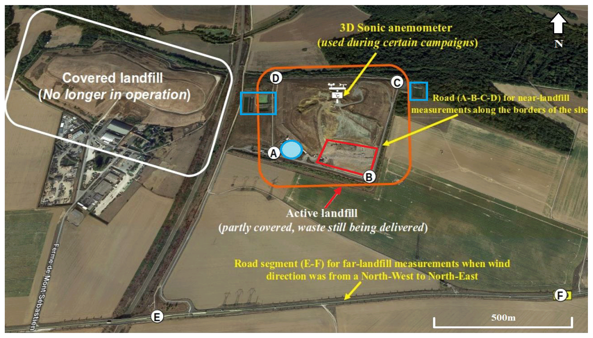
Figure 1Satellite image (source: © Google Earth) of the studied landfill (orange rectangle on the right side of the figure), an older closed landfill (white rectangle on the left), and its surrounding area. The red quadrangle, blue rectangles, and blue circle designate the locations of the active landfill cell during the period 2018–2020, the leachate ponds, and the biogas valorization plant, respectively. The letters A to F designate the ends of the segments of the roads along which the mobile measurements were taken during the field measurements. Most of the measurements were taken along the road segments A to B and B to C close to the landfill or along the E to F remote roads, which are henceforth referred to as EF (E and F refer to the end-points of any distant sampling road; however, the measurements only from EF remote roads south of the landfill were used for inversions). During most of the campaigns, a 3-D sonic anemometer was installed at an elevated location near the center of the landfill.
The topography of the landfill is complex. It may be generally described as a hill that rises towards the center and slopes away towards the edge. The highest point of the landfill is a few tens of meters above the outer edges, with variations in time due to the evolution of the landfill. The area surrounding the landfill is generally flat as it has been used as cropland. The closed landfill exhibits similar topography to the studied one with a similar height and a slightly greater extent (area ∼ 0.25 km2; Fig. 1). Based on measurement surveys conducted previously (Vogel, 2016) and during this study, we see that there is no significant CH4 signal from this closed landfill in our measurements targeting the active landfill.
2.2 Scientific instrumentation
2.2.1 Mobile ground laboratory and sniffing measurement framework
Atmospheric sampling was performed within and around the studied landfill using an MGL. A vehicle was equipped with one to three gas analyzers that continuously measured the in situ CH4 mole fraction, the mole fraction of additional trace gases (CO2, CO, C2H2, H2O), and isotope mole fractions (δ13C in CH4 and δ13C in CO2) depending on the type of analyzer (Fig. 2). We utilized a variety of high-precision cavity-enhanced absorption spectroscopy gas analyzers: the Picarro G2203 (CH4, C2H2, H2O), G2401 (CH4, CO2, CO, H2O), and G2201-i (CH4, CO2, δ13C in CH4, and δ13C in CO2), which use cavity ring down spectrometry; the ABB Ultra-portable Greenhouse Gas Analyzer (ABB-UGGA) and Micro-portable Greenhouse Gas Analyzer (ABB-MGGA), which use off-axis integrated cavity output spectroscopy; and a LI-COR LI-7810 prototype gas analyzer, which uses optical-feedback cavity-enhanced absorption spectroscopy (see Table 1). The accuracy of all gas analyzers was verified in the laboratory using low (1.98 ± 0.11 (1σ) ppm) and high (6.14 ± 0.23 (1σ) ppm) CH4 mole fraction calibration standards that are traceable to World Meteorological Organization (WMO) greenhouse gas scales (WMOX2004A; Crotwell et al., 2019).
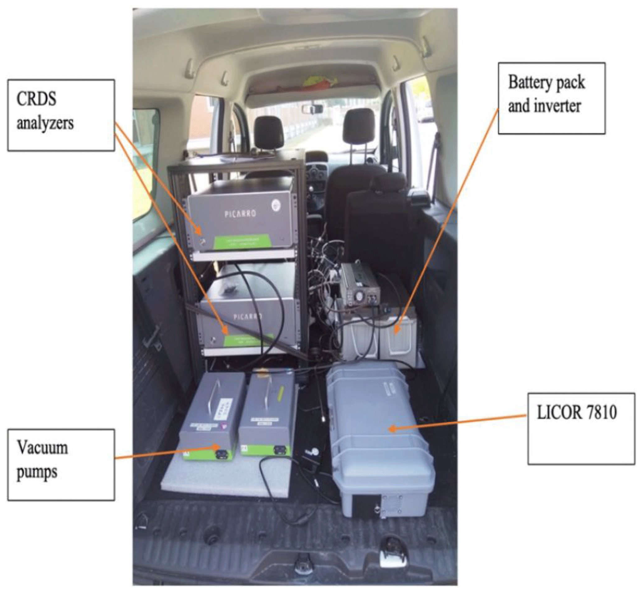
Figure 2Example of the mobile instrument configuration as set up in a vehicle. Different combinations of instruments were used for the different campaigns, as detailed in Table 1. The LICOR™ 7810 in the picture was on loan to LSCE and was used in one campaign only.
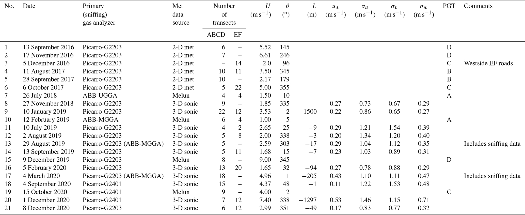
Table 1Summary of all 21 MGL measurement campaigns and corresponding atmospheric conditions, averaged values of the meteorological and turbulence parameters over the campaign period (mean horizontal wind speed (U) and direction (θ), the Obukhov length (L), surface friction velocity (u∗), and standard deviation of wind velocity fluctuations (σu, σv, σw) and Pasquill–Gifford–Turner (PGT) stability classes when the high-frequency measurements from the 3-D sonic were unavailable).
The gas analyzers were connected to an air inlet located towards the front of the MGL roof using in. Synflex 1300 tubing. Power was supplied by gel lead-acid batteries (12 V, 150 Ah) with either one battery connected directly to a power inverter (12 V/230 V, DC/AC) or two batteries connected in series (24 V/230 V, DC/AC). A Global Positioning Satellite (GPS) module inside the MGL recorded the sampling position at 1 Hz during the campaigns. All measurements were synchronized to UTC. Moreover, the net gas analyzer time response (including the delay induced by the sampling line) was initially determined on site by providing a short burst of breath into the air inlet and then timing the response for post-correction of the campaign data set.
2.2.2 Meteorological measurements
Reliable meteorological and micrometeorological measurements are required to support the analysis of the gas mole fraction measurements and, in particular, to characterize atmospheric conditions in the Gaussian plume dispersion model used for the inversion modeling to estimate CH4 emissions from the landfill. For the MGL measurement campaigns during 2016–2017, a two-dimensional (2-D) anemometer meteorological station, measuring 1 min averaged wind speed and direction, was permanently installed at ∼ 10 m height above ground level (a.g.l.) near the biogas valorization plant (Fig. 1). For the majority of campaigns between 2018 and 2020, a three-dimensional (3-D) sonic anemometer (Gill Instruments WindMaster 3-Axis Anemometer) was installed near the center and the highest point of the landfill where nearby obstacles were limited. The anemometer was installed on a mast at a height of between about 2 to 7 m a.g.l. Data from the 3-D sonic anemometer were recorded at 20 Hz using a Raspberry Pi 3B+ logging computer. For 4 of the 21 campaigns documented in this study, wind measurements were not made on site, and, therefore, computations relied on wind observation data from the nearby Melun meteorological station (48∘36′37′′ N, 2∘40′46′′ E) operated by Meteo France, which is located ∼ 5.5 km SW of the studied landfill. For all campaigns, we used atmospheric pressure, air temperature, and humidity measurements from the Melun station.
2.3 Measurement strategy
The monitoring of the CH4 emissions from the landfill site posed two major challenges related to spatiotemporal variability: (a) that of the identification of the different methane sources on the site, which can either be very localized (hotspots) or more diffuse sources, and (b) that of the estimation of their emissions, which can vary over time due to changing operational or external parameters, e.g., atmospheric conditions. In order to tackle these challenges, the main strategy for our measurement campaigns was (a) to continuously measure CH4 mole fractions across the atmospheric plumes downwind of the landfill (obtaining plume cross-sections) during MGL surveys of at least 1 h along roads close to and distant from the site and (b) to conduct some on-foot sniffing within the landfill to identify local methane hotspots and to characterize the potential emissions sources. The longer-term (seasonal and interannual) temporal variability was also addressed by conducting campaigns over several years. MGL campaigns were performed on the road along the perimeter of the site between points A, B, C, and D in Fig. 1 and/or along the EF remote roads, where E and F refer to the end-points of any distant sampling road. Due to accessibility limitations of suitable EF remote roads, the campaigns generally targeted days when winds were from the northwest to the northeast to ensure that the mobile transects on the EF remote roads south to the landfill lay downwind of the site and would intersect the landfill CH4 emission plume. The measurements conducted on these southern EF remote roads (subsequently referred to as EF roads) are primarily used for inversions. When planning the campaigns, such suitable meteorological conditions were chosen from weather forecasts at least a day in advance. All campaigns were carried out between mid-morning and early afternoon on weekdays when the site could be accessed.
2.4 General information on the campaigns
We conducted a total of 27 MGL campaigns between September 2016 and December 2020, with an average period of revisit of ∼ 42 d, ranging between 7 and 149 d. However, the measurements made during six MGL campaigns are excluded from the study because, during these campaigns, the GPS MGL position was not recorded, which prevented us from conducting robust analysis. Therefore, we conducted our analysis for the 21 campaigns listed in Table 1. During two of these MGL campaigns (29 August 2019 and 4 March 2020), we simultaneously conducted additional foot-based sniffing measurements at the ground level within and around the site for locating specific point or area sources within the landfill site. In both sniffing campaigns, a portable ABB MGGA was used to measure CH4 mole fractions, with a GPS positioning module, whilst walking around suspected hotspots within the landfill. We obtained an average of about 10 plume cross-sections per campaign. For 11 of these 21 MGL campaigns, we have plume cross-sections on EF roads which were used in the inverse modeling framework (Sect. 4) for the estimation of the total methane emissions from the landfill. Sampling was performed along the ABCD road (see Fig. 1) in all but one of the 21 MGL campaigns under a variety of different wind conditions. This sampling aimed to provide insight into the spatial distribution of emissions within the landfill, but we also expected that plume cross-sections along these roads could support the inversion of the total emission from the landfills or from some of its main areas of emissions, in particular from its different cells.
Table 1 summarizes information on the gas analyzers used, the number of ABCD and/or EF plume cross-sections conducted, and the meteorological and/or turbulence parameters for all the selected 21 campaigns. For each selected campaign, Figs. S1.2 to S1.22 show the CH4 mole fraction time series, plume cross-sections, and the corresponding wind conditions according to on-site meteorological measurements or local wind conditions in four campaigns from the Melun weather station. The wind speed (U) and wind direction (θ) for each campaign are averaged over each campaign period. The averaged wind speeds in all of the selected campaigns varied from ∼ 1 to ∼ 7 m s−1 (Table 1). During two of the 21 campaigns, averaged wind speeds were equal or below 1.5 m s−1. The use of a Gaussian plume model for such low wind speed conditions leads to higher uncertainty in CH4 emission estimates (Kumar et al., 2021, 2022). However, during these campaigns, we had CH4 measurements along the EF road that appeared to be suitable, and we still attempted inversions to estimate the CH4 emissions from the site with these measurements. During several campaigns, CH4 mole fraction measurements were made even when unfavorable winds were coming from the east to the southwest directions (Table 1). The mobile transects in these campaigns were mostly conducted along the ABCD road and/or along a westside EF remote road, very near to the landfill. In other campaigns, the wind directions ranged between the northwest and northeast directions, which enabled us to use MGL sampling on both the ABCD and EF roads (Table 1).
Whenever the high-frequency data from the 3-D sonic anemometer were available, the essential turbulence parameters, the Obukhov length (L), surface friction velocity (u∗), and standard deviation of wind velocity fluctuations (σu, σv, σw) were computed over each campaign period. All of the campaigns were conducted during daytime, and, thus, for the campaigns with 3-D sonic data, the negative sign and magnitude of the Monin–Obukhov stability parameter () indicate that the atmospheric stability varied from near-neutral to unstable and very unstable conditions. For the remaining campaigns, the Pasquill–Gifford–Turner (PGT) atmospheric stability classes, characterized based on the wind measurements (Turner, 1970), varied from neutral (PGT class D) to very unstable (PGT class A) conditions.
The background CH4 mole fraction outside the plume cross-sections conducted along ABCD and EF roads in each campaign was taken as the first percentile of the CH4 measurements so that the enhancements in CH4 due to landfill emissions could be determined from this background. Measurements obtained upwind of the landfill, usually between points C and D (Fig. 1), confirmed that using the first percentile was appropriate to characterize the background CH4 field, on top of which lies the plumes from the landfill. This approach of deriving a background from field measurements eliminates any potential offset issues in the gas analyzers, thereby reducing instrumental uncertainty.
Across all the 21 selected campaigns, the maximum CH4 enhancement above the background reached up to ∼ 70 and ∼ 3.5 ppm for the ABCD and EF roads, respectively. We computed averages of the CH4 mole fraction enhancements for segments of these roads from the different mobile transects along them. To compute these averages, a road was divided into equidistant segments with an averaged distance interval between the measurement locations. Then, the CH4 mole fractions at each segment point were averaged by using the nearest-point CH4 mole fraction values from different mobile transects. These averaged CH4 mole fractions are shown in Fig. 3 for the EF roads and in Figs. S1.2–S1.22 for all the roads. During most of the campaigns when the wind was blowing from the direction of northwest to northeast, the high CH4 mole fraction enhancements represented either individual plume cross-sections or averaged CH4 plumes and were observed along the road segments A–B or B–C (Figs. S1.2 to S1.22). The averaged CH4 plumes from different campaigns along the ABCD road systematically showed multiple CH4 peaks at nearly the same downwind locations during the series of MGL cross-sections. These different CH4 peaks indicate the heterogeneous distribution of CH4 emissions within the landfill. The different plume cross-sections and corresponding averaged CH4 plume along the EF road show a more unimodal plume distribution in most of the campaigns (Fig. 3). Measurements at this distance allow the whole landfill to be considered as a single CH4 emission source.
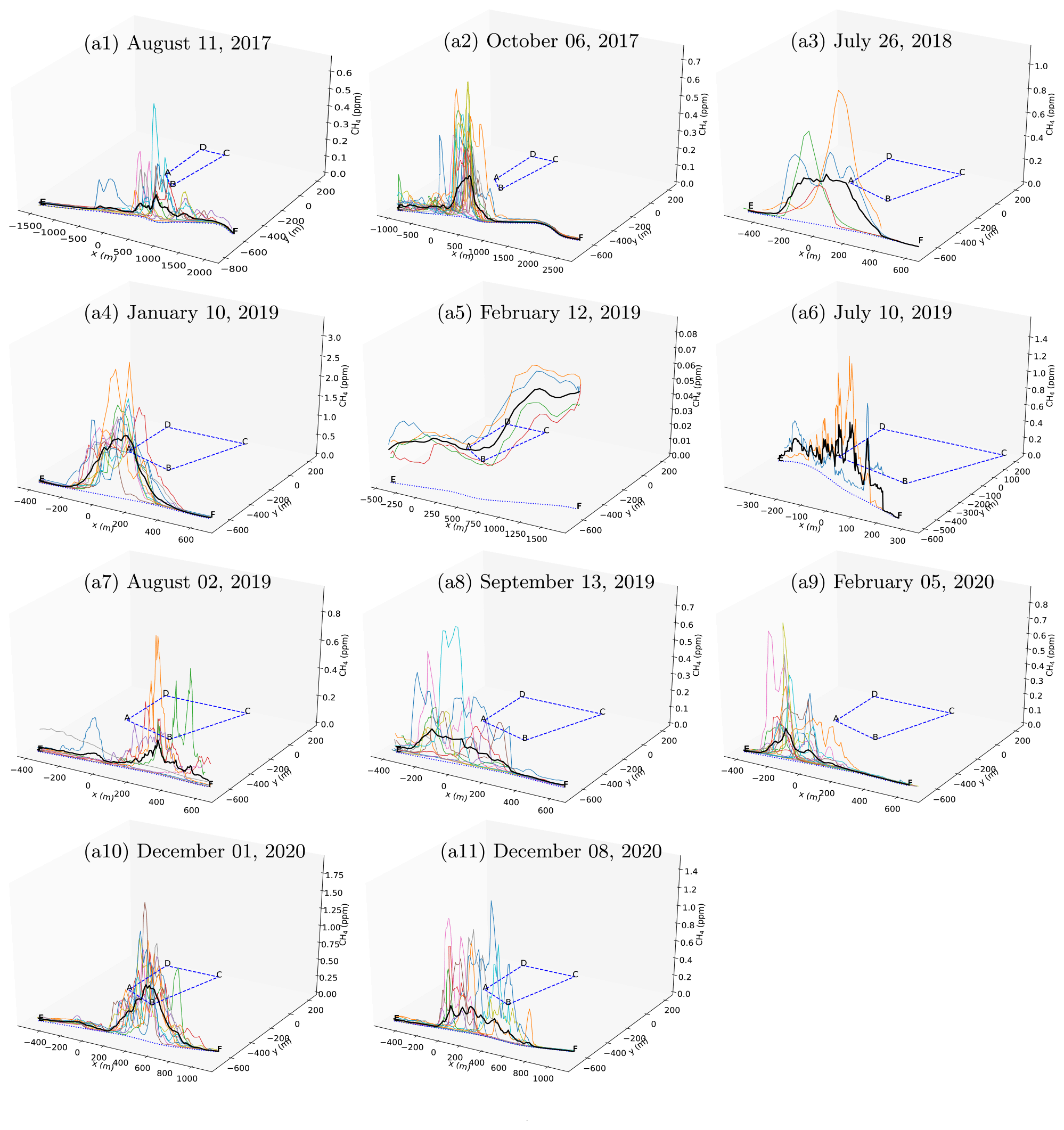
Figure 3Enhancement of CH4 mole fractions above the background in different plume cross-sections along the EF roads during different measurement campaigns. The solid black line shows the averaged CH4 mole fractions computed from the different plume cross-sections in each campaign.
A rough knowledge a priori of (or assumptions on) the position and extent of the major CH4 sources within the landfill are needed to set up the inversion configurations or to strengthen the results from the inversions: whether the emissions correspond to a set of point sources or relatively large area sources and whether some areas tend to emit more than the others as a function of the period when the campaigns are conducted. Point and/or area sources within the landfill originate from biogas pipes, well heads, damaged membranes, the biogas power plant, active and/or covered cells, leachate ponds, etc. However, a priori knowledge of the spatial distribution of methane emissions within the studied landfill was very limited before the sniffing campaigns. In a previous study to quantify emissions from the same landfill using mobile measurements from two campaigns (17 November and 5 December 2016), Albergel et al. (2017) divided the site into five potential emission areas. This definition of potential area sources was based on rough information from the landfill operators and did not account for potential emissions from the biogas valorization plant, leachate ponds, or the pipe or well network. In this study, we conducted two sniffing campaigns by foot and relied on these to identify the principal methane hotspots (Sect. 3.1). Furthermore, we performed a detailed analysis of the measurements conducted at the borders of the landfill along the ABC road from different mobile campaigns combined with corresponding wind speeds and directions to explore if these could provide some insights about the potential CH4 emission sources within the landfill or on their spatial representativity.
3.1 Identification of CH4 hotspots from the sniffing campaigns
We analyzed measurements from the foot-based sniffing campaigns on 29 August 2019 and 4 March 2020 to identify the potential methane hotspots and their source origin. It is important to recognize that, during these sniffing campaigns, CH4 mole fraction measurements were often obtained very close to the source, and, therefore, high mole fraction observations do not necessarily correspond to equally large fluxes.
Figure 4a shows the spatial distribution of CH4 mole fractions along the measurement path from the sniffing campaign on 29 August 2019. Six locations with high CH4 peaks, at least ∼ 30 m apart from each other, were identified (Fig. 4b). These locations were examined with a detailed map of the biogas collection pipes, wells, leachate ponds, gas processing facilities, etc. to identify their source origin. Based on this analysis, we found that the two hotspots S1 and S2 are near biogas network purges, S4 is located near a biogas network well, S5 is at the location of a bioreactor tank, and S6 is near a leachate bioreactor or biogas purge where landfill gas is removed from the landfill cells and also close to a major junction of biogas pipes. The hotspot S3 is near to a leachate well and also downwind of a biogas network and a well. The methane peaks in different mobile plume transects on the ABC road during this campaign (Fig. S1.14c) are consistent with these six hotspots within the landfill.
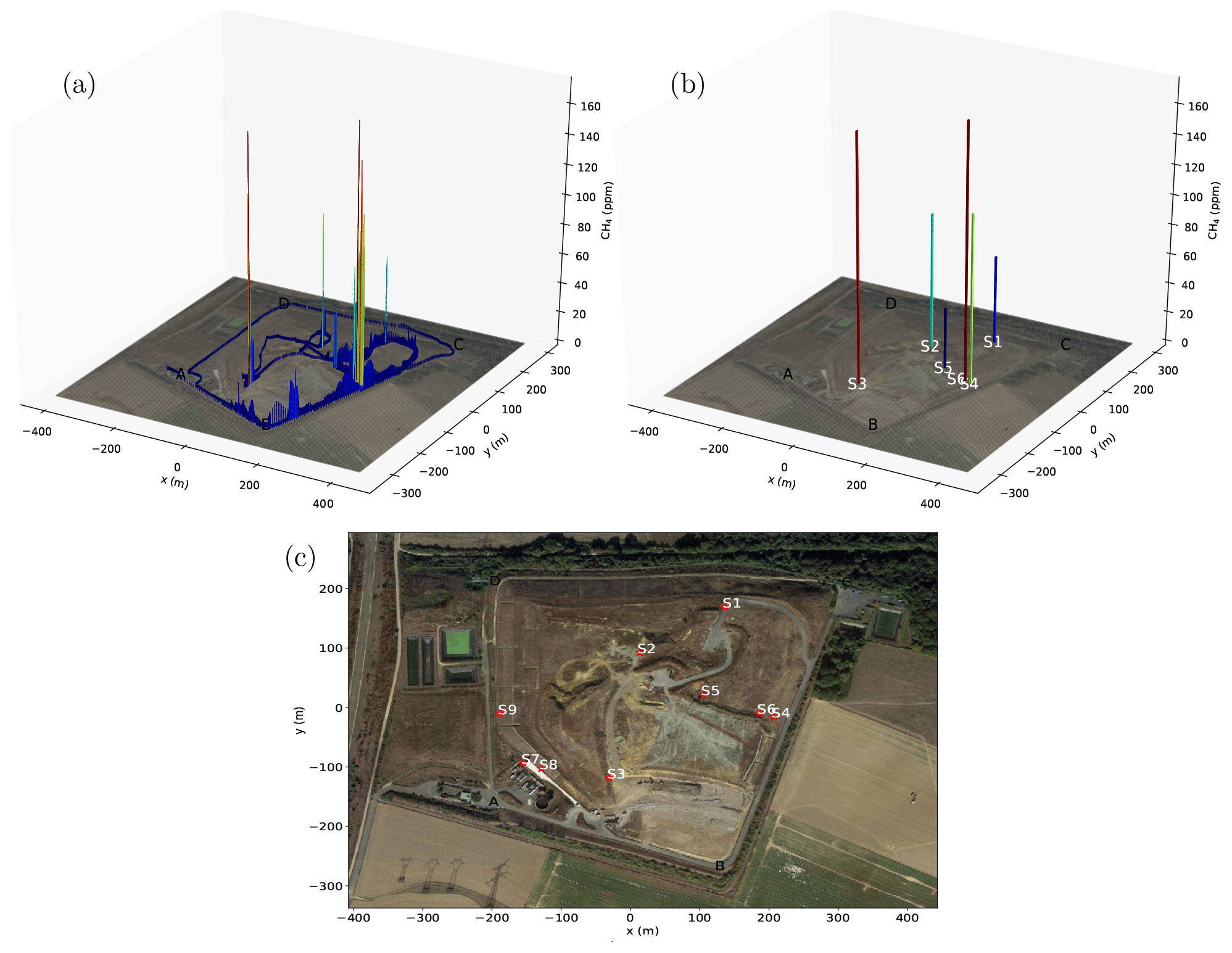
Figure 4(a) Observed CH4 mole fractions from sniffing on 29 August 2019 within the studied landfill using an ABB MGGA along with a GPS module and (b) high CH4 mole fraction peaks from the sniffing data are assumed to correspond to the main emission hotspots: six of them are identified during this campaign (S1 to S6). Panel (c) shows the locations of a total of nine emission hotspots (S1 to S9) identified from both the sniffing campaigns on 29 August 2019 and 4 March 2020. The underlying aerial photograph background images are taken from Google Earth (© Google Earth).
The results of the sniffing campaign on 4 March 2020 confirmed CH4 hotspots at similar locations (S1 to S6) to those observed on 29 August 2019. Additional measurements obtained near biogas network wells; a biogas network purge (S9) and two along a drainage gutter behind the biogas power plant (S7 and S8) (Fig. 4c) indicated three more hotspots with measured methane mole fractions in the range of 60 to 800 ppm. Therefore, we identified a total of nine hotspots (S1 to S9) from the analysis of the two sniffing campaigns (Fig. 4c). These nine potential methane emission point sources were used in the inversion tests to estimate their emissions. It is important to note that the rapid ability to identify leaks from these sniffing campaigns provides an opportunity for site operators to easily diagnose methane emissions and take actions to reduce them whilst also increasing the yield of CH4 that is captured and available for sale or use on site.
3.2 Directional information on potential CH4 emission sources from the plume cross-sections along the ABC road
Other than the two sniffing campaigns, which offered a snapshot insight into localized emission sources, little information is available about the presence and characteristics of emissions within the landfill. To gain more insights, we analyzed the plumes collected along the ABC road under various wind conditions from different campaigns. A first analysis of the ABC measurements from different mobile campaigns indicates a similarity of the plume cross-sections along this road despite changes in wind direction from one campaign to the next (Figs. S1.1–S1.21). It indicates that these measurements are more representative of both the localized leakages from pipes and wells near to these roads than of the emissions from the greater landfill. Furthermore, we constructed bivariate polar plots from all the plume cross-sections along the ABC road from the 11 campaigns between July 2018 and December 2020, where on-site wind data from the 3-D sonic anemometer were available (Table 1; Fig. 5). These bivariate polar plots can provide useful directional information on the potential emission sources and may help to identify the presence and characteristics of these sources (Carslaw and Beevers, 2013).

Figure 5Bivariate polar plots of the mean CH4 mole fraction enhancement above background in seven equidistant segments (Seg-1 to Seg-7) obtained from mobile transects during 11 campaigns between July 2018 and December 2020 along the ABC road. Each polar plot in a segment uses the values of CH4 mole fractions averaged over the duration of the part of each mobile transect in that segment. Nine red stars (S1 to S9) indicate the key CH4 hotspots identified from two sniffing campaigns.
The bivariate polar plots from the ABC plume cross-sections are constructed in the following way. The ABC road is divided into seven segments (Seg-1 to Seg-7), and for each segment, CH4 mole fraction enhancements above the background are averaged over the duration of each transect in that segment. Wind speed and direction measurements are averaged over durations starting from 1 min prior to a transect in a segment until the end of the transect in that segment. The averaged wind speeds, wind directions, and mole fraction data are partitioned into wind speed and direction bins, and the mean CH4 mole fractions are calculated for each bin. The mean CH4 mole fractions in each wind-speed–direction bin are plotted using polar coordinates. We used wind direction intervals at 22.5∘ and wind speed intervals at 1 m s−1 for binning the data in each bivariate polar plot. The mean CH4 mole fractions, calculated in wind-speed–direction bins with limited data points, such that those with one,two, and three points are down-weighted with the weights 0.25, 0.50, and 0.75, respectively (Carslaw and Beevers, 2013).
Figure 5 shows the seven bivariate polar plots in each segment (Seg-1 to Seg-7) along the ABC road. These bivariate plots provide different directional information on the likely methane emission sources contributing to the methane mole fractions in different segments. The polar plot in Seg-1 suggests that at least two small sources were present just north of this segment (near the biogas power plant), as indicated by the elevated mean CH4 mole fractions in the bins with northerly winds when wind speeds were moderate (∼ 4–6 m s−1). One of the sniffing campaigns on 4 March 2020 also identified two hotspots (S7 and S8) in this area along a drainage gutter behind the plant (Fig. 4c, Sect. 3.1). The polar plots in Seg-2 to Seg-6 indicate multiple emission sources within the whole landfill with potentially high emitting sources corresponding to Seg-2 and Seg-3 and small sources corresponding to Seg-4 to Seg-6. The high CH4 mole fractions in the northerly wind direction bins in Seg-2, 3, and 4 are strongly influenced and most probably caused by the last, uncovered, active cell of the landfill in the southeast corner. The plots in Seg-2 to Seg-6 also indicate some local emission sources near the roads, from the high mean CH4 mole fractions in the bins of low wind speeds. High CH4 mole fractions in the northerly wind direction bins in the polar plot in Seg-5 indicate potential CH4 emission sources that could correspond to hotspots S4 and S6, identified by the sniffing campaigns. The polar plot in Seg-7 has a small number of data points and does not indicate any major source upwind of the segment. The polar plots in Seg-4 to Seg-6 also show some unexpected elevated mean CH4 mole fractions in the bins with northeast wind directions and moderate wind speeds, which indicates potential emitting sources in the northeast, outside the landfill. However, there are only agriculture farms in the northeast of these segments of the landfill, where we do not expect any major methane sources, except only minor methane emissions from using fertilizers or manure, which are unlikely to explain such enhanced CH4 mole fractions. The ABC road follows the border of the landfill with localized leakages from pipes and wells near to these roads, and half of the road segments (A–B and B–C) are adjacent to a steep ridge in the southeast. Therefore, recirculation of the wind flow due to these ridges and the complex landfill topography may explain these observations. The transport of a plume in a complex flow field along the B–C road, especially when the wind is blowing from the direction of northeast to southeast, does not follow the observed mean wind directions. As the air from northeasterly or easterly wind directions is deflected against the ridges of the landfill, it is possible that high CH4 mole fractions may be measured along the B–C road, even though the air would appear to originate from outside the landfill.
This analysis of the polar bivariate plots substantiates the evidence of methane hotspots identified from the sniffing campaigns (Sect. 3.1). Furthermore, these results question the ability of the ABC measurements, which might be strongly impacted by sources located along the roads, to spatially represent the emissions from the greater landfill. This would hamper the use of these data for inverting landfill emissions. The complex atmospheric transport along the ridge also raises large uncertainties in inversions using this data with a simple Gaussian model (Sect. 5.1).
3.3 Definition of potential emission sources within the landfill for inversion tests
The detection of hotspots during the two sniffing campaigns within the landfill (Sect. 3.1) and the analysis of the mobile measurements along the ABC road in different wind conditions from different campaigns (Sect. 3.2) indicate that landfill methane emissions come from a combination of area and point sources. Consequently, we develop several inversion configurations, one of which defines the potential sources as the nine hotspots identified from the sniffing (Sect. 3.1, Fig. 4c), while others correspond to the area sources (Fig. 6). The analysis of the CH4 enhancements measured along the ABC road provided only qualitative directional information on the area and/or point sources within the landfill (Sect. 3.2). However, due to the complex nature of the landfill and the spatiotemporal variability of emissions, it is uncertain whether we have detected all the hotspots through sniffing, and identifying the area sources of emissions with more dispersed emissions is exceedingly challenging. As a consequence, we have chosen to define a set of large area sources with uniformly distributed methane emissions for inversions. Thus, we defined six potential emission source regions, i.e., six area sources that include the biogas power plant (A-1) and the five cells (A-2 to A-6) within the landfill (Fig. 6).
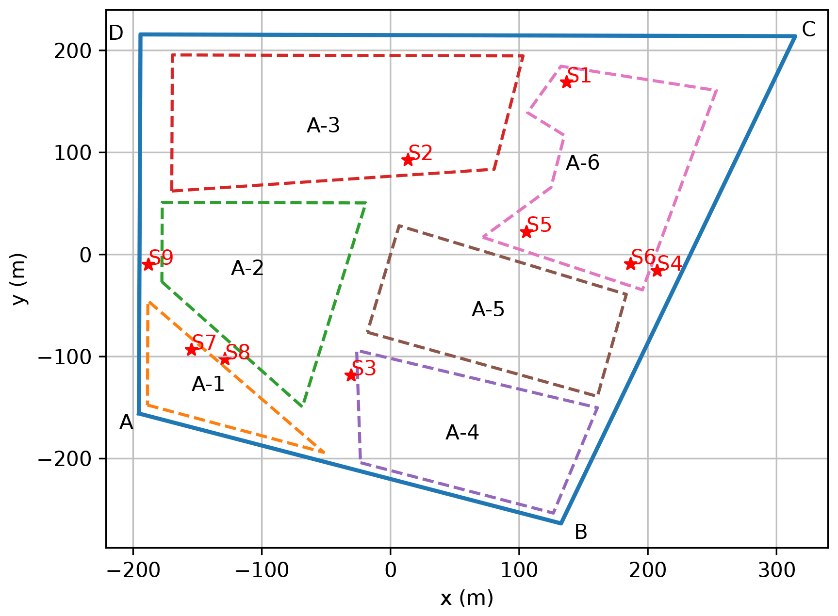
Figure 6The six potential area sources (boxes, A-i, ) in the configuration of the inversion, defined as the biogas valorization plant (A-1) and the five cells (A-2 to A-6). Nine red stars (S1 to S9) indicate the CH4 hotspots identified from two sniffing campaigns.
We used a simple atmospheric inversion framework to quantify CH4 emissions from multiple potential sources within the landfill using the MGL measurements. The inversion exploits some of the basic theoretical and practical components of the approaches described in Kumar et al. (2022, 2021) and Ars et al. (2017) and uses the assumption about the characterization of potential CH4 emissions sources from Sect. 3. We used a Gaussian plume dispersion model designed for single point sources from Kumar et al. (2021, 2022) for estimating emissions from the nine CH4 hotspots as point sources (Sect. 3.2) and adapted the same Gaussian model to simulate the dispersion from area sources when estimating emissions from the six area sources (Sect. 3.3). Details on the Gaussian plume model equations for a point source dispersion and their adaptation to an area source dispersion are provided in the Supplement 2 (Sect. S2.1). We describe two different approaches to formulate the Gaussian model for an area source dispersion: method 1 is a very simple approach that modifies the lateral plume spread in relation to the total plume width as a sum of the plume spread due to atmospheric turbulence and of the additional initial spread due to the source size (Sect. S2.1.1a), and method 2 decomposes an area source into multiple point sources and superimposes the modeled Gaussian plumes from all of these point sources to compute the average plume from that area (Sect. S2.1.1b).
When on-site measurements from a meteorological station (3-D sonic anemometer or 2-D) were available, the Gaussian model was driven by the averaged wind direction given by the meteorological data. When relying on the data from the Melun station, the mean wind direction was approximately taken as a direction from the center of the landfill to the location of the maximum averaged CH4 mole fraction (Kumar et al., 2021). This wind direction approximation was deemed to be more representative of the landfill rather than of the Melun wind direction, and we evaluated the effect of this approximation on the estimates in Sect. 5.2. In all cases, the model is driven by the effective mean wind speed from the meteorological data (Sect. S2.1). The dispersion parameters in the Gaussian model are defined by the standard deviations of the velocity fluctuations (σv, σw) when we have the high-frequency 3-D sonic data available, and in other cases (four campaigns), they are based on the Briggs dispersion formulas for flat terrain (Briggs, 1973) corresponding to the defined PGT stability classes. We used the Gaussian model to simulate the plume (called the response function) of each potential CH4 source separately at the measurement locations, with atmospheric conditions observed during the averaging periods of ABC and/or EF plume transects and using a unitary emission rate (1 kg s−1). A response function defines a linear relationship between the emission rate of a potential source and the concentration at a measurement location.
We used a non-negative least-squares minimization approach to formulate the inverse problem for the quantification of unknown emissions of multiple potential emission sources. The details of this inversion procedure are provided in the Supplement (Sect. S2.2). The principle of the inversion process is to minimize the root sum squared misfits between the averaged observed and modeled mole fraction enhancements in the plumes from the multiple potential sources. These inversions rely on a priori information about the potential emission sources (e.g., number, type, location, size, and/or shape), the response functions simulated with the Gaussian model for each potential emission source, and the observation vectors of the measured and modeled plumes. We employed two options to define the observation vectors in the inversion. The first observation vector (μpt) is defined as the averaged CH4 mole fractions at the measurement locations along the roads. Since we have to estimate multiple sources of methane emissions within the landfill site, following Ars et al. (2017), we discretize the roads into multiple segments of equal length, and for each segment, the integrated areas under the averaged CH4 mole fractions are used to define a different observation vector (μSI). This approach reduces the tendency of the inversion to over-fit turbulent patterns within the plume. We divide the plumes into a different number of segments on the ABC and EF roads with 50 and 100 m distance intervals, respectively. More information about these observation vectors is given in the Supplement (Sect. S2.2).
For both ABC and EF roads, we conducted six inversion tests using two types of observation vectors (μpt and μSI) for three source configurations. The source configurations involve nine point sources (hotspots identified from the sniffing campaigns, as discussed in Sect. 3) and six area sources (Sect. 3) modeled by two different area source adaptations of the Gaussian model (method 1 and method 2).
We conducted inversion tests for all of the selected campaigns when the wind conditions allowed us to obtain plume cross-sections on ABC (near-field) and/or EF roads (far-field). However, it is challenging to model the plume cross-sections along the ABC road using a simple Gaussian plume dispersion model and, therefore, to invert the site emissions based on the data measured on this road. The dispersion of CH4 from the potential sources to the ABC road is highly sensitive to the complex topography of the landfill, which is not taken into account in the Gaussian modeling. The vicinity between this road and the potential sources in the landfill makes these measurements also highly sensitive to factors such as the a priori information on the location and extent of the potential emission sources, while Sect. 3 shows that we can hardly provide a precise distribution of the sources within the landfill. Finally, Sect. 3.2 highlighted our lack of understanding of the spatial representativity of the measurements along the ABC road. The inversions using data from the ABC road are thus likely hampered by large uncertainties and need to be analyzed cautiously, but they may provide insights into the spatial distribution of the emissions. On the contrary, the shape of the observed averaged plume along the EF roads is almost unimodal in most of the campaigns, and the Gaussian model should be more suitable for the modeling of the transport over the distance between the potential sources within the landfill and the EF road. Therefore, we do not expect the inversions based on the data from the EF road to provide better insights into the spatial distribution of the emissions compared to the ABC road; however, we expect them to provide much more robust estimates of the total emissions from the landfill than those based on the data from the ABC road.
The campaign of 10 January 2019 is taken as an example to illustrate the analysis of the data and the inversions. The Gaussian model for this campaign is driven by the measured meteorological and turbulence parameters from the on-site 3-D sonic anemometer data. Wind directions during this campaign were mainly from the north which allowed us to get 22 and 12 CH4 plume cross-sections on the ABC and EF roads, respectively (Table 1, Fig. S1.10). Furthermore, the absolute magnitude of the Obukhov length (L) computed from the 3-D sonic data is greater than 1000 m (Table 1), which suggests neutral atmospheric stability conditions during this campaign. The averaged CH4 mole fraction plume along the ABC road shows multiple peaks (Fig. S1.10), whereas the averaged plume along the EF road is unimodal (Fig. 3a4). Observed enhancements of the averaged CH4 plumes above the background reached up to ∼ 25 and ∼ 1.5 ppm along the ABC and EF roads, respectively.
The division of the observed and modeled plumes over sub-segments of ABC and EF roads (to build μSI) from the 10 January 2019 campaign is illustrated in Figs. 7a1 and b1 and 8a1 and b1, respectively. Figures 7b1 and 8b1 illustrate a comparison of the modeled plumes with method 1 and method 2 from each potential area source at the measurement roads ABC and EF, respectively. For the ABC road, the shapes of modeled plumes from two different methods for the area sources A-1 to A-3 (which are a little farther from the ABC road) are approximately similar. However, noticeable differences in the shapes and magnitudes (i.e., horizontal spread) can be seen in the modeled plumes from the sources A-4 to A-6, which are closer to the measurement road ABC. The method-2 plumes are slightly narrower and have a larger maximum than those from method 1. Figure 8b1 for the EF measurements shows that the behavior of modeled plumes from both methods is approximately similar and unimodal. Some differences can be noticed in terms of magnitude and width, with method-2 plumes being slightly narrower and having a larger maximum than method 1 (Fig. 8b1).
5.1 Emission estimates using ABC road measurements
Figure 7 illustrates the inverted emissions using measurements from the ABC road for the campaign of 10 January 2019. The total estimated CH4 emissions using μpt and μSI in the inversion tests with nine hotspots are 22.94 and 22.82 t CH4 d−1, respectively. The total emissions using μpt (and μSI) and using six area sources with method 1 and method 2 are 12.98 (13.09) and 13.83 (13.56) t CH4 d−1, respectively. Figure 7a2 and b2 show that the fit between the observed and modeled μpt from the Gaussian model using the corresponding emission estimates with six areas sources are slightly better than those from the nine hotspots. The inversion using nine hotspots assigns the estimated emissions to the three point sources that lie in two source areas, A-6 and A-3, only (Fig. 7a3), whereas the estimated emissions from the inversion using six area sources are approximately equally distributed to three area sources A-4, A-5, and A-6 (Fig. 7b3). It is noticed that the total estimates are weakly sensitive to the observation vector μpt or μSI. However, the discrepancy between the estimated emissions obtained with different definitions of the potential emission sources and also from different implementations of area sources (method 1 and method 2) in the inversion tests is noticeable. The absolute differences between the estimated emissions using nine point sources and six area sources in the inversions are ∼ 10 and ∼ 9 t CH4 d−1 for method 1 and method 2, respectively.
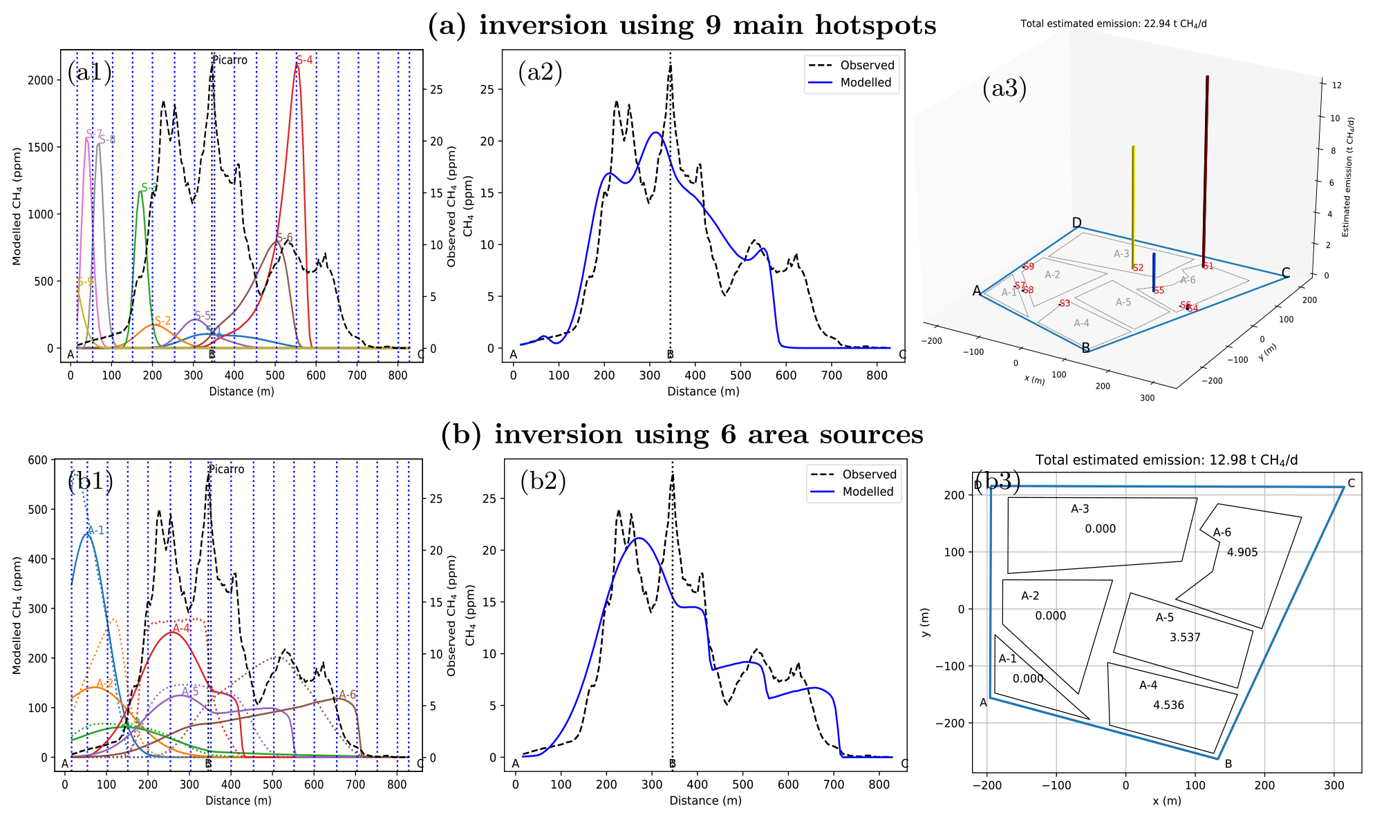
Figure 7An example of modeling the individual plumes and emission rates from the inversion tests using (a) nine main hotspots and (b) six area sources with μpt from the measurements obtained along the ABC road on 10 January 2019. From left to right in each row, the first to third columns plots respectively show (1) the average CH4 mole fraction enhancements above the background (dashed black line, right y axis) and modeled response functions (solid colored lines for method 1 and the same colored dotted lines for method 2, left y axis) for each potential source, (2) the fit between the observed (dashed black lines) and modeled (solid blue lines) CH4 mole fraction enhancements, and (3) estimates of the CH4 emissions (t CH4 d−1) for each of the potential sources. Vertical dotted blue lines in the first column figures show the point of division of the roads into sub-segments over which the averaged mole fractions are integrated to define μSI.
For most of the selected campaigns using data from the ABC road, we observed a similar behavior by the estimated CH4 emissions from different inversion tests as from the results from the 10 January 2019 campaign. The estimated emissions using ABC data from different campaigns vary between ∼ 2 to ∼ 36 t CH4 d−1 using six area sources and ∼ 4 to ∼ 23 t CH4 d−1 using nine point sources in different inversion tests (Fig. S2.1). The estimates show large biases in the orders of magnitude between total methane emission estimates from different tests. The large differences in the inverted total CH4 emissions using different definitions of the potential sources in the inversion tests show a high sensitivity of the estimates to a priori information about potential sources.
We analyzed the spatial distribution of methane emission estimated from the inversions using ABC measurements. Figure S2.16 shows the spatial distributions of the estimated CH4 emissions attributed to the individual source regions from the inversions using six area sources and μpt from the ABC measurements from all the selected campaigns. This shows that the two source areas A-1 and A-2 have negligible contributions to the total estimated methane emissions. Emissions from sources A-3 to A-6 are more regularly inferred from most of the campaigns. Emissions from A-3 are variable and may indicate a highly variable source, while emissions from A-4 are more consistent, which may be expected as this area of the landfill was active during this time. High methane emissions attributed to the A-6 source region during some of the campaigns may be emitted from the methane hotspots identified from the foot sniffing campaigns near the biogas network purges, biogas network well, and bioreactor tank (Sect. 3.1).
5.2 Emission estimates using EF road measurements
For the campaign of 10 January 2019, the total estimated CH4 emissions using μpt and μSI from EF road measurements in the inversions with nine hotspots are 4.50 and 3.98 t CH4 d−1, respectively. The total estimated CH4 emissions using μpt (and μSI) and six area sources with method 1 and method 2 are 4.44 (4.41) and 4.16 (4.18) t CH4 d−1, respectively. Figure 8a2 and b2, respectively, for nine hotspots and six area sources with μpt in the inversions show a good agreement between the observed and modeled CH4 mole fractions from the dispersion model using the corresponding inverted emissions. The estimated CH4 emissions from the inversions with method 1 and method 2 for an area source implementation in the Gaussian model have a small percentage difference of ∼ 6 % using either μpt or μSI. The inversion results using EF measurements are weakly sensitive to the defined observation vectors μpt and μSI with ∼ 12 % and less than ∼ 1 % percentage differences in flux estimates from nine hotspots and six area sources, respectively. The total estimated methane emissions using nine hotspots and six area sources with μpt had small percentage differences of ∼ 1 % and ∼ 8 % for method 1 and method 2, respectively. Figure 8a3 shows that, in the inversion using nine hotspots, the estimated emissions are distributed only to three point sources in two source areas, A-6 and A-4. In contrast, the inversion using six area sources assigns the estimated emissions primarily to A-6, with small contributions from A-5 and A-4, as shown in Fig. 8b3.
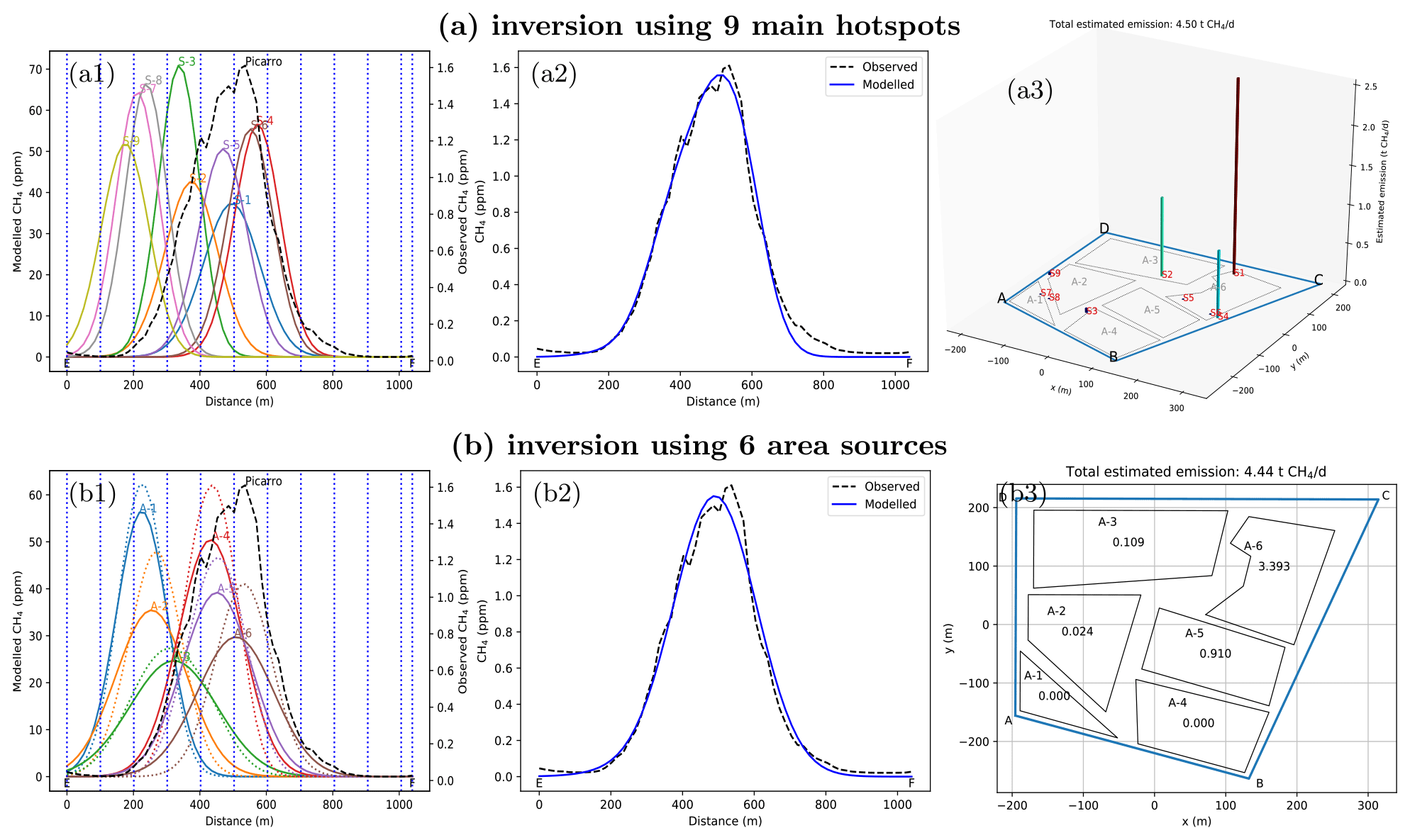
Figure 8An example of modeling the individual plumes and emission rates from the inversion tests using (a) nine main hotspots and (b) six area sources with μpt from the measurements obtained along the EF road on 10 January 2019. From left to right in each row, first to third columns plots, respectively, show (1) the average CH4 mole fraction enhancements above the background (dashed black line, right y axis) and modeled response functions (solid colored lines for method 1 and the same colored dotted lines for method 2, left y axis) for each potential source, (2) the fit between the observed (dashed black lines) and modeled (solid blue lines) CH4 mole fraction enhancements, and (3) estimates of the CH4 emissions (t CH4 d−1) for each of the potential sources. Vertical dotted blue lines in the first column figures show the point of division of the roads into sub-segments over which the averaged mole fractions are integrated to define μSI.
We conducted another sensitivity analysis of the inversion results with respect to a different definition of the five rectangular potential area sources defined within the five cells (Fig. S2.2), as proposed by Albergel et al. (2017). Using these five area sources and with μpt obtained from the EF measurements from 10 January 2019, the total estimated emissions (4.24 and 4.19 t CH4 d−1 with method 1 and method 2, respectively) (Fig. S2.3) have small percentage differences (∼ 4 % and ∼ 1 %) compared to the total estimated emissions (4.44 and 4.16 t CH4 d−1 for method 1 and method 2, respectively) obtained using six area sources in inversions. In order to analyze the effect of the approximated wind direction (Sect. 4) on inversion results when relying on the meteorological data from Melun met station in the Gaussian model, we tested this assumption for the campaign on 10 January 2019, where, instead of using actual observed wind direction, we forced the model to use the wind direction approximation. With μpt, total estimated emissions of 4.03 and 3.80 t CH4 d−1 using nine hotspots and six area sources, respectively, have ∼ 11 % and ∼ 15 % differences compared to those obtained using the actual observed mean wind direction from the local 3-D sonic anemometer (4.50 and 4.44 t CH4 d−1, respectively). Overall, different sensitivity tests using EF measurements from 10 January 2019 indicate that the percentage differences between the total estimated emissions range from less than 1 % to ∼ 15 %. This suggests that the total estimated emissions exhibit weak sensitivity to different input parameters in the inversion tests.
Figure 9 shows the estimated total methane emissions from the studied landfill using μpt obtained from the EF measurements from the 11 campaigns where sampling was conducted on the southern EF road. These estimations are based on using nine hotspots as prior point sources and six potential area sources, with two different methods (method 1 and method 2) for area source implementation in the Gaussian model. Figures S2.3–S2.14 present more details about these inversion results. The total CH4 emissions using nine hotspots from the inversions vary from 0.44 t CH4 d−1 (5 February 2020) to a maximum of 6.90 t CH4 d−1 (1 December 2020), with an average emission of 2.24 t CH4 d−1. These estimates are similar to the estimated emissions obtained using six area sources with method 1 (and method 2) which vary from 0.34 (0.34) to 7.04 (6.30) t CH4 d−1, with an average value of 2.07 (2.00) t CH4 d−1.
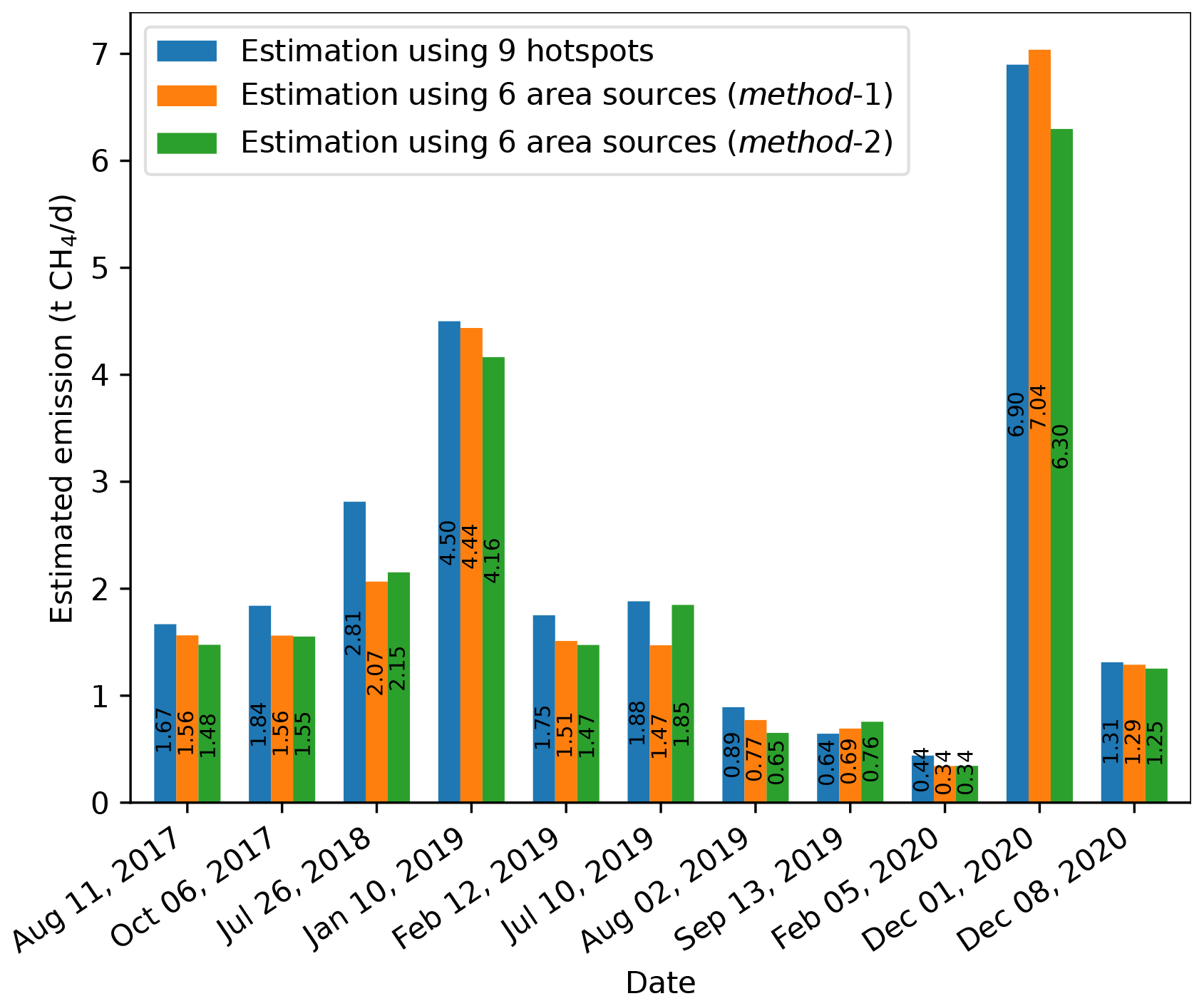
Figure 9Summary of the total estimated CH4 emissions using the observation vector μpt obtained from EF road data and using nine hotspots from sniffing as point sources and six area sources with two different methods (method 1 and method 2) for area source implementation in the Gaussian model.
Similarly to the inversion results using EF measurements from the 10 January 2019 campaign, the results from different inversion tests using three different definitions of the potential emissions sources, two observation vectors, and two different implementations of the area sources in the Gaussian plume model show that the percentage differences between the total estimated emissions from different combinations of these tests averaged over the 11 campaigns ranged from ∼ 1 % to ∼ 15 %. This analysis shows that the emission estimates using EF measurements are weakly sensitive to the different definitions of potential emission sources, observation vectors, and other parameters considered in the inversion tests. Thus, based on this analysis, we consider it to be that the total estimated methane emissions using the EF measurements are robust. The estimates obtained through ABC measurements in inversions are much higher compared to the estimates from the EF road. These ABC estimates are highly sensitive to different characterizations of potential sources (Sect. 5.1) due to various factors such as the complex landfill topography, the inability to account for it in the Gaussian model, our limited understanding of the spatial representativity of potential sources, the short distances between measurements and potential sources, etc. This weakens our confidence in the estimates derived from the data collected along the ABC road. Therefore, we rely on the estimates obtained using measurements from the EF road for the estimation of landfill methane emissions.
We also analyzed the spatial distribution of the estimated emissions from the EF road measurements. Figure S2.17 shows that the inversions using EF measurements assign a significant proportion of net methane emissions to the A-6 area source (Fig. 6), along with some contributions from A-4 and A-5. EF measurements additionally attributed a small part of total methane emissions to the A-1 source area, which includes the biogas plant and was not detected by the inversions using ABC measurements.
The averages of total CH4 emissions using data from EF measurements from all 11 campaigns (where suitable MGL sampling was conducted) vary from ∼ 2.0 to ∼ 2.2 t CH4 d−1 in different inversion sensitivity tests. This indicates that the use of remote mobile plume cross-section measurements is suitable for quantification of the total methane emissions from the site, which are weakly sensitive to the characterization of the potential emission sources and other influencing parameters like the observation vectors, wind directions, etc. Thus, these results highlight the necessity of conducting measurements at a sufficient distance from the landfill to obtain a reliable estimate of total methane emissions, minimizing the influence of landfill topography. However, this increased distance makes it challenging to discern the spatial distribution of emissions within the landfill. On the other hand, the inversion tests performed with sampling from the landfill perimeter (ABC) show a high sensitivity of the estimates to the spatial distribution of the potential emission sources and other parameters in the inversions. It highlights the difficulties in exploiting ABC measurements to estimate CH4 emissions using a simple Gaussian plume model due to the model's inability to consider complex landfill topography and lack of precise information about potential emission sources. Thus, estimates using the ABC road were deemed to be poorly representative of actual landfill methane emissions. However, the ABC measurements taken in proximity to the landfill are shown to be useful to identify and rank the main emission areas, i.e., to get insights into the spatial distribution of the emissions within the landfill. This demonstrates the complementarity between the near- and far- field measurements.
The total CH4 emissions using data from the EF road show a large temporal variability (∼ 0.4 to ∼ 7 t CH4 d−1) in landfill methane emissions (Fig. 9). The emission sources and thus the methane emissions from an active landfill can vary greatly even over a small period of a few days. For example, total methane emissions on 8 December 2020 (∼ 1.25 t CH4 d−1) were far smaller than on 1 December 2020 (∼ 7 t CH4 d−1) despite a 1-week interval between these two sampling campaigns and despite the fact that measurements were conducted during daytime hours of between 11:30 to 12:30 UTC in both campaigns. We anticipate that the high temporal variability in the emissions is primarily attributable to landfill activity, such as the fixing of a large methane leak, which can lead to a substantial drop in emissions within a short timeframe. However, the limited availability of day-to-day activity data for this landfill makes it challenging to attribute the variability in our emission estimates based on the EF measurements to particular landfill activities. Thus, more mobile campaigns on the EF road are required to more accurately monitor and to better understand temporal variabilities of landfill methane emissions. Note that the estimates from each of the selected campaigns are based on the measurements spanning an order of 1 to 2 daytime hours. However, different atmospheric conditions and landfill activities during nighttime and other daytime hours may contribute to a diurnal pattern in landfill emissions (Sonderfeld et al., 2017). To better understand the diurnal variability of landfill methane emissions, we need to monitor the emissions at a higher temporal resolution. For this, continuous automated measurements at a certain distance of the site over long periods are required, which is impractical using a labor-intensive MGL unless the MGL were to be permanently installed in a vehicle that travels along the EF transect frequently. Continuous CH4 mole fraction measurements from a network of fixed sensors around a site alongside meteorological measurements can provide an alternative to develop an automated monitoring system to monitor long-term landfill methane emissions at a higher temporal resolution. However, the deployment of a dense network of high-precision sensors is still limited by cost. Recently, Riddick et al. (2018) utilized a single-point continuous CH4 measurement that was sampled ∼ 700 m downwind from a landfill, and they combined this with a Lagrangian particle model to estimate the methane emissions at a high temporal resolution. A similar approach can be applied to monitor landfill methane emissions for short- and long-term temporal-variability studies. Such an approach could be complemented by other techniques, such as MGLs, which may provide complementary information on the spatial variability of sources within the landfill and which may be more suited to leak detection and mitigation.
A limitation of our inversion approach is that it does not diagnose explicit estimates of the uncertainties in the estimated CH4 emissions. Extrapolating the results obtained with a similar approach applied to controlled-CH4-release experiments during the TADI-2018 and TADI-2019 campaigns (Kumar et al., 2022, 2021), we assume that our emission estimates from the EF road have a level of uncertainty of ∼ 30 %. The errors diagnosed during TADI's controlled-release experiments were mainly applicable for flat terrain conditions. Here, much of the plume dispersion from the landfill to the measurements transects occurs over flat terrain. However, the landfill itself corresponds to a complex topography. We currently lack information on the errors from Gaussian plume dispersion models when applied to such a terrain, making it difficult to provide a more robust diagnostic of uncertainties in our estimates.
Several studies have shown that the temporal variability of landfill methane emissions is driven by absolute or temporal gradients of some meteorological parameters, especially atmospheric pressure (Czepiel et al., 2003; Poulsen et al., 2003; Xu et al., 2014; Aghdam et al., 2019; Kissas et al., 2022). A limited number of studies, like Riddick et al. (2018), have demonstrated a very weak negative or no clear relationship between landfill CH4 emissions and changes in atmospheric pressure. We also analyzed these emission–pressure or emission–temperature relationships using the estimated CH4 emissions from the EF road measurements and the atmospheric pressure and temperature measured at Melun station (Fig. S2.15). We observed a weak negative correlation of landfill methane emissions with atmospheric pressure () and a slightly stronger negative correlation with atmospheric temperature () (Fig. S2.15). Riddick et al. (2018) discussed several possible contributing factors to this weak emission–pressure relationship, such as ongoing landfill operations on an active landfill during a measurement campaign and emission data gaps. These are reasonable contributory factors in our case of the studied active landfill as the sample size of our landfill emission estimates is very small, with large data gaps between emission estimates.
For near-landfill measurements on the ABCD road, methane plumes coming from the sources within the landfill are generally not well mixed, either horizontally or vertically, as they are too close to the emission sources. The discrete landfill emission sources at higher elevations may not be detected within these measurements, with the sampling air intake at ∼ 2 m above the ground surface. Recirculation of the wind flow due to complex landfill topography affects the transport and dispersion of mixing methane plumes at the measurement positions, which is difficult to simulate with a simple Gaussian plume model that considers spatially homogeneous flow. Thus, the estimation of methane emissions using these measurements requires a more complex model that can resolve the flow field and turbulence induced by the complex topography of the landfill. Computational fluid dynamics (CFD) models are more suitable for such applications and have been used to simulate high-resolution flow fields and turbulence in complex terrains. These CFD models could provide opportunities to account for variations in the flow field in space and time. However, the computational cost of such a model for emission inversions will be high compared to a simple Gaussian approach.
As discussed above, despite the large uncertainties in net emissions estimated using ABC measurements, these estimates together with the sniffing campaigns provide some information on the spatial distribution of emissions within a landfill and thus insights into the relative contribution of the different areas and types of activities occurring within the landfill to the total landfill emissions. The spatial distributions of CH4 emissions from individual source regions revealed two main source areas (A-4 and A-6) and two other areas (A-5 and A-3) with lesser emissions that contributed to the total estimated methane emissions for most of the campaigns. The inversions using EF measurements strengthened the assumption that the A-6 source area is one of the main contributors to net methane emissions, with additional contributions from A-3, A-4, and A-5 and a small proportion of total methane emissions from the A-1 source area. A-5, A-6, and A-3 were covered with clay and membrane during most of the campaigns, but there were junctures of biogas network wells, bioreactor tanks, etc. within these source areas. As discussed in Sect. 3.1 with the analysis of near-surface sniffing measurements, many of the identified hotspots were near to these components, which contributed to a majority of the methane emissions from these source areas. We observed significant temporal variability in the emissions from this source area (Fig. S2.16), and this variation underscores the fact that the elevated emissions primarily coincide with instances of sporadic leakages in potential emitting infrastructures in the landfill. However, the source area A-4 was the last sector where waste reception was ongoing during this study, particularly in the last phase of the campaigns when we had reliable on-site meteorological measurements to support the analysis of the emission spatial distribution within the landfill using the ABC measurements. During active waste reception, the corresponding reception areas, here A-4, are open and uncovered, and A-4 was thus restricted from any sniffing measurements due to safety considerations. However, the analyses with the ABC measurements and with the inversions identified A-4 as one of the continuous emitters and as the largest source area on average, which is consistent with the fact that the waste in this area is already producing biogas which is not collected (or only partially) because of limited biogas network systems in this area and because of the lack of final cover. As the areas on the southwestern side of the landfill have been the first areas to be filled, the methane emissions are significantly lower in this part. The covering is designed to improve biogas capture for electricity production on site. However, the methane production in the newest areas and the leaks in the landfill infrastructure may explain the higher emissions on the northern and eastern sides (A-3, A-4, A-5, and A-6) of the landfill. Measurements with a terrain-resolving flow and dispersion model may provide better information about the spatial distribution of emission sources within the landfill as these would better replicate sniffing campaigns similar to those described in this study.
The information about the distribution of the emission sources from the inversions and the hotspots identified from the sniffing campaigns helps site operators to prioritize mitigation actions (cover improvement, improvement of landfill gas network collection, etc.). Typically, at landfill sites, emission sources are highly variable in space and time, with individual sources within the landfill ranging from sporadic to continuous and from spatially heterogenous hotspots to large diffusive areas. The analysis of measurements and inversions from the different MGLs help to provide some qualitative information about the potential emission sources, but their ability to precisely locate the exact spatial distribution of these sources is limited by the distance between the vehicle (road) and the sources. Regular sniffing campaigns by foot or by drone using a portable analyzer and GPS module help, to some extent, to locate certain suspected hotspots.
Our long-term monitoring of landfill methane emissions required significant resources and effort. It would have been challenging to conduct a similar effort for other landfills. Additional studies, like this one, will be essential for establishing robust standard atmospheric monitoring techniques applicable to diverse landfills. Further research is needed to refine the generic emission factors for landfill methane emissions in methane emission inventories. However, we managed to link the main part of the emissions to the waste-tipping area which remains uncovered over a long period of time with limited biogas collection systems. This type of result should provide useful information to site managers with regard to effective mitigation actions and improved landfill operation management. Our measurement strategy and inversion approaches are generalizable for the monitoring of emissions from other landfills, providing a basis for future applications and development.
In this study, we present long-term, near-surface mobile measurements from 21 campaigns for reliable quantification of total methane emissions from an active landfill using atmospheric inversion modeling. We applied a simple inversion approach to quantify methane emissions from the landfill using a Gaussian plume model. Measurements from a remote EF road, further away from the landfill, were preferable for inverse modeling as the estimates based on these measurements were proven to be only weakly sensitive to the defined potential emission sources and other influencing parameters in the inversions. The total CH4 emissions estimated using different definitions of potential sources and using data where sampling was conducted on the distant EF road (11 campaigns) varied from ∼ 0.4 to ∼ 7 t CH4 d−1, with an average flux value of ∼ 2.1 t CH4 d−1. These estimated landfill methane emissions showed large temporal variability. Emission estimates based on the measurements conducted along the perimeter of the landfill (ABC) were very sensitive to the characterization of potential emission sources and were limited in their ability to provide representative landfill emission estimates. However, the analysis of these measurements, as well as those from the sniffing campaigns within the landfill site, helped to identify the main landfill emission areas. This information remained insufficient to define the detailed spatial distribution of the emission sources within the site. However, it showed that the two main area sources correspond respectively to a covered waste sector with infrastructure with sporadic leakages (such as wells, tanks, pipes, etc.) and to the last active sector receiving waste during most of the measurement campaigns. This demonstrates the complementarity between the near- and far-field measurements. Based on our estimated landfill emissions using EF road measurements, we found a weak negative correlation between emissions and atmospheric pressure and a slightly stronger inverse relationship between emissions and atmospheric temperature. To better characterize such relationships and also for more accurate monitoring of landfill emissions, we suggest that emission estimates should be maintained on longer-term measurements, ideally measurements that are made continuously. In order to better utilize these measurements for landfill emission quantification, especially when sampling close to the landfill, we suggest using a more complex model, such as a CFD model, that can resolve the flow field and turbulence induced by the complex landfill topography.
The data and code are accessible upon reasonable request.
The supplement related to this article is available online at: https://doi.org/10.5194/amt-17-1229-2024-supplement.
PK conducted the data analysis and implemented the inverse modeling system and performed the model simulations and inversions. GB and PK designed the inverse modeling system, and the LSCE members participated in the design of the observation strategy. CC and AS organized the main series of the measurement campaigns. CC, CYK, SWG, AS, OL, SA, SD, LL, ML, JDP, and FV conducted the campaigns and processed the data together with PK. PK, GB, and CC prepared and reviewed the paper with critical contributions from AS, PC, OL, and all the other co-authors. All the co-authors participated in the discussions regarding the results.
The contact author has declared that none of the authors has any competing interests.
Publisher’s note: Copernicus Publications remains neutral with regard to jurisdictional claims made in the text, published maps, institutional affiliations, or any other geographical representation in this paper. While Copernicus Publications makes every effort to include appropriate place names, the final responsibility lies with the authors.
We would like to thank the SUEZ site staff for their assistance in the measurement campaigns. We also acknowledge IFP Energies nouvelles-Géoscience, France, for participating in some of the campaigns.
This research has been supported by Chaire Industrielle TRACE (grant no. ANR-17-CHIN-0004-01), which is cofunded by the French National Research Agency (ANR), TOTAL Raffinage Chimie, SUEZ, and Thales Alenia Space (TAS).
This paper was edited by Abhishek Chatterjee and reviewed by two anonymous referees.
Aghdam, E. F., Scheutz, C., and Kjeldsen, P.: Impact of meteorological parameters on extracted landfill gas composition and flow, Waste Manage., 87, 905–914, https://doi.org/10.1016/j.wasman.2018.01.045, 2019.
Albergel, A., Morin, D., Buty, D., Nibart, M., Makke, L., Goix, R., Kelly, R., Bouchet, C., and Vogel, F.: Inverse dispersion modelling for a quick scan service to assess fugitive emissions from landfills, in: 18th International Conference on Harmonisation within Atmospheric Dispersion Modelling for Regulatory Purposes, Bologna, Italy, http://www.harmo18.eu/ (last access: 13 February 2024), 2017.
Allen, G., Hollingsworth, P., Kabbabe, K., Pitt, J. R., Mead, M. I., Illingworth, S., Roberts, G., Bourn, M., Shallcross, D. E., and Percival, C. J.: The development and trial of an unmanned aerial system for the measurement of methane flux from landfill and greenhouse gas emission hotspots, Waste Manage., 87, 883–892, https://doi.org/10.1016/J.WASMAN.2017.12.024, 2019.
Ars, S.: Caractérisation des émissions de méthane à l'échelle locale à l'aide d'une méthode d'inversion statistique basée sur un modèle gaussien paramétré avec les données d'un gaz traceur, Université Paris Saclay (COmUE), France, https://theses.hal.science/tel-01624241 (last access: 17 March 2023), 2017.
Ars, S., Broquet, G., Yver Kwok, C., Roustan, Y., Wu, L., Arzoumanian, E., and Bousquet, P.: Statistical atmospheric inversion of local gas emissions by coupling the tracer release technique and local-scale transport modelling: a test case with controlled methane emissions, Atmos. Meas. Tech., 10, 5017–5037, https://doi.org/10.5194/amt-10-5017-2017, 2017.
Ars, S., Vogel, F., Arrowsmith, C., Heerah, S., Knuckey, E., Lavoie, J., Lee, C., Pak, N. M., Phillips, J. L., and Wunch, D.: Investigation of the Spatial Distribution of Methane Sources in the Greater Toronto Area Using Mobile Gas Monitoring Systems, Environ. Sci. Technol., 54, 15671–15679, https://doi.org/10.1021/acs.est.0c05386, 2020.
Bel Hadj Ali, N., Abichou, T., and Green, R.: Comparing estimates of fugitive landfill methane emissions using inverse plume modeling obtained with Surface Emission Monitoring (SEM), Drone Emission Monitoring (DEM), and Downwind Plume Emission Monitoring (DWPEM), J. Air Waste Manage., 70, 410–424, https://doi.org/10.1080/10962247.2020.1728423, 2020.
Bingemer, H. G. and Crutzen, P. J.: The production of methane from solid wastes, J. Geophys. Res.-Atmos., 92, 2181–2187, https://doi.org/10.1029/JD092iD02p02181, 1987.
Bogner, J. and Matthews, E.: Global methane emissions from landfills: New methodology and annual estimates 1980–1996, Global Biogeochem. Cy., 17, 1065, https://doi.org/10.1029/2002gb001913, 2003.
Bogner, J., Spokas, K., Burton, E., Sweeney, R., and Corona, V.: Landfills as atmospheric methane sources and sinks, Chemosphere, 31, 4119–4130, https://doi.org/10.1016/0045-6535(95)80012-A, 1995.
Bogner, J., Pipatti, R., Hashimoto, S., Diaz, C., Mareckova, K., Diaz, L., Kjeldsen, P., Monni, S., Faaij, A., Qingxian, G., Tianzhu, Z., Mohammed, A. A., Sutamihardja, R. T. M., and Gregory, R.: Mitigation of global greenhouse gas emissions from waste: Conclusions and strategies from the Intergovernmental Panel on Climate Change (IPCC) Fourth Assessment Report. Working Group III (Mitigation), Waste Manage. Res., 26, 11–32, https://doi.org/10.1177/0734242X07088433, 2008.
Bourn, M., Robinson, R., Innocenti, F., and Scheutz, C.: Regulating landfills using measured methane emissions: An English perspective, Waste Manage., 87, 860–869, https://doi.org/10.1016/j.wasman.2018.06.032, 2019.
Bousquet, P., Ciais, P., Miller, J. B., Dlugokencky, E. J., Hauglustaine, D. A., Prigent, C., van der Werf, G. R., Peylin, P., Brunke, E. G., Carouge, C., Langenfelds, R. L., Lathière, J., Papa, F., Ramonet, M., Schmidt, M., Steele, L. P., Tyler, S. C., and White, J.: Contribution of anthropogenic and natural sources to atmospheric methane variability, Nature, 443, 439–443, https://doi.org/10.1038/nature05132, 2006.
Briggs, G. A.: Diffusion estimation for small emissions, ATDL contribution file no. 79, National Oceanic and Atmospheric Administration, Oak Ridge, Tennessee, https://doi.org/10.2172/5118833, 1973.
Cambaliza, M. O. L., Shepson, P. B., Bogner, J., Caulton, D. R., Stirm, B., Sweeney, C., Montzka, S. A., Gurney, K. R., Spokas, K., Salmon, O. E., Lavoie, T. N., Hendricks, A., Mays, K., Turnbull, J., Miller, B. R., Lauvaux, T., Davis, K., Karion, A., Moser, B., Miller, C., Obermeyer, C., Whetstone, J., Prasad, K., Miles, N., and Richardson, S.: Quantification and source apportionment of the methane emission flux from the city of Indianapolis, Elementa: Science of the Anthropocene, 3, 000037, https://doi.org/10.12952/journal.elementa.000037, 2015.
Carslaw, D. C. and Beevers, S. D.: Characterising and understanding emission sources using bivariate polar plots and k-means clustering, Environ. Modell. Softw., 40, 325–329, https://doi.org/10.1016/j.envsoft.2012.09.005, 2013.
Crotwell, A., Lee, H., and Steinbacher, M. (Eds.): 20th WMO/IAEA meeting on carbon dioxide, other greenhouse gases and related measurement techniques (GGMT-2019), GAW report No. 255, World Meteorological Organization, Geneva, Switzerland, 2019.
Czepiel, P. M., Mosher, B., Harriss, R. C., Shorter, J. H., McManus, J. B., Kolb, C. E., Allwine, E., and Lamb, B. K.: Landfill methane emissions measured by enclosure and atmospheric tracer methods, J. Geophys. Res.-Atmos., 101, 16711–16719, https://doi.org/10.1029/96JD00864, 1996.
Czepiel, P. M., Shorter, J. H., Mosher, B., Allwine, E., McManus, J. B., Harriss, R. C., Kolb, C. E., and Lamb, B. K.: The influence of atmospheric pressure on landfill methane emissions, Waste Manage., 23, 593–598, https://doi.org/10.1016/S0956-053X(03)00103-X, 2003.
Daugėla, I., Suziedelyte Visockiene, J., and Kumpiene, J.: detection and analysis of methane emissions from a landfill using unmanned aerial drone systems and semiconductor sensors, Detritus, 10, 127–138, https://doi.org/10.31025/2611-4135/2020.13942, 2020.
Dreyfus, G. B., Xu, Y., Shindell, D. T., Zaelke, D., and Ramanathan, V.: Mitigating climate disruption in time: A self-consistent approach for avoiding both near-term and long-term global warming, P. Natl. Acad Sci. USA, 119, e2123536119, https://doi.org/10.1073/pnas.2123536119, 2022.
Duan, Z., Hansen, P. O. C. R., Scheutz, C., and Kjeldsen, P.: Mitigation of methane and trace gas emissions through a large-scale active biofilter system at Glatved landfill, Denmark, Waste Manage., 126, 367–376, https://doi.org/10.1016/j.wasman.2021.03.023, 2021.
Duan, Z., Scheutz, C., and Kjeldsen, P.: Mitigation of methane emissions from three Danish landfills using different biocover systems, Waste Manage., 149, 156–167, https://doi.org/10.1016/J.WASMAN.2022.05.022, 2022.
Emran, B. J., Tannant, D. D., and Najjaran, H.: Low-altitude aerial methane concentration mapping, Remote Sens.-Basel, 9, 823, https://doi.org/10.3390/rs9080823, 2017.
Etminan, M., Myhre, G., Highwood, E. J., and Shine, K. P.: Radiative forcing of carbon dioxide, methane, and nitrous oxide: A significant revision of the methane radiative forcing, Geophys. Res. Lett., 43, 12614–12623, https://doi.org/10.1002/2016GL071930, 2016.
European Commission: COMMUNICATION FROM THE COMMISSION TO THE EUROPEAN PARLIAMENT, THE COUNCIL, THE EUROPEAN ECONOMIC AND SOCIAL COMMITTEE AND THE COMMITTEE OF THE REGIONS on an EU strategy to reduce methane emissions, Brussels, COM(2020) 663 final, https://eur-lex.europa.eu/legal-content/EN/TXT/PDF/?uri=CELEX:52020DC0663 (last access: 17 March 2023), 2020.
European Environment Agency: Annual European Union greenhouse gas inventory 1990–2018 and inventory report 2020, UNFCCC Secretariat, EEA/PUBL/2022/023, https://www.eea.europa.eu/publications/annual-european-union-greenhouse-gas-1 (last access: 17 March 2023), 2020.
European Union Methane Action Plan: European Union Methane Action Plan – Policies – IEA, https://www.iea.org/policies/17024-european-union-methane-action-plan (last access: 17 March 2023), 2022.
Fischedick, M., Roy, J., Acquaye, A., Allwood, J., Ceron, J.-P., Geng, Y., Kheshgi, H., Lanza, A., Perczyk, D., Price, L., Santalla, E., Sheinbaum, C., and Tanaka, K.: Industry, in: Climate Change 2014: Mitigation of Climate Change. Contribution of Working Group III to the Fifth Assessment Report of the Intergovernmental Panel on Climate Change, edited by: Edenhofer, O., Pichs-Madruga, R., Sokona, Y., Farahani, E., Kadner, S., Seyboth, K., Adler, A., Baum, I., Brunner, S., Eickemeier, P., Kriemann, B., Savolainen, J., Schlömer, S., von Stechow, C., Zwickel, T., and Minx, J. C., Cambridge University Press, Cambridge, United Kingdom and New York, NY, USA, 739–810, 2014.
Fjelsted, L., Christensen, A. G., Larsen, J. E., Kjeldsen, P., and Scheutz, C.: Assessment of a landfill methane emission screening method using an unmanned aerial vehicle mounted thermal infrared camera – A field study, Waste Manage., 87, 893–904, https://doi.org/10.1016/j.wasman.2018.05.031, 2019.
Foster-Wittig, T. A., Thoma, E. D., Green, R. B., Hater, G. R., Swan, N. D., and Chanton, J. P.: Development of a mobile tracer correlation method for assessment of air emissions from landfills and other area sources, Atmos. Environ., 102, 323–330, https://doi.org/10.1016/j.atmosenv.2014.12.008, 2015.
Fox, T. A., Barchyn, T. E., Risk, D., Ravikumar, A. P., and Hugenholtz, C. H.: A review of close-range and screening technologies for mitigating fugitive methane emissions in upstream oil and gas, Environ. Res. Lett., 14, 53002, https://doi.org/10.1088/1748-9326/ab0cc3, 2019.
Gasbarra, D., Toscano, P., Famulari, D., Finardi, S., di Tommasi, P., Zaldei, A., Carlucci, P., Magliulo, E., and Gioli, B.: Locating and quantifying multiple landfills methane emissions using aircraft data, Environ. Pollut., 254, 112987, https://doi.org/10.1016/j.envpol.2019.112987, 2019.
Hartmann, D. L., Tank, A. M. G. K., Rusticucci, M., Alexander, L. v, Brönnimann, S., Charabi, Y. A. R., Dentener, F. J., Dlugokencky, E. J., Easterling, D. R., Kaplan, A., Soden, B. J., Thorne, P. W., Wild, M., and Zhai, P. M.: Observations: Atmosphere and Surface, in: Climate Change 2013: The Physical Science Basis. Contribution of Working Group I to the Fifth Assessment Report of the Intergovernmental Panel on Climate Change, edited by: Stocker, T. F., Qin, D., Plattner, G.-K., Tignor, M., Allen, S. K., Boschung, J., Nauels, A., Xia, Y., Bex, V., and Midgley, P. M., Cambridge University Press, Cambridge, United Kingdom and New York, NY, USA, 159–254, 2013.
Hein, R., Crutzen, P. J., and Heimann, M.: An inverse modeling approach to investigate the global atmospheric methane cycle, Global Biogeochem. Cy., 11, 43–76, https://doi.org/10.1029/96GB03043, 1997.
Hong, J., Chen, Y., Wang, M., Ye, L., Qi, C., Yuan, H., Zheng, T., and Li, X.: Intensification of municipal solid waste disposal in China, Renew. Sust. Energ. Rev., 69, 168–176, https://doi.org/10.1016/j.rser.2016.11.185, 2017.
Jackson, R. B., Saunois, M., Bousquet, P., Canadell, J. G., Poulter, B., Stavert, A. R., Bergamaschi, P., Niwa, Y., Segers, A., and Tsuruta, A.: Increasing anthropogenic methane emissions arise equally from agricultural and fossil fuel sources, Environ. Res. Lett., 15, 071002, https://doi.org/10.1088/1748-9326/ab9ed2, 2020.
Jha, A. K., Sharma, C., Singh, N., Ramesh, R., Purvaja, R., and Gupta, P. K.: Greenhouse gas emissions from municipal solid waste management in Indian mega-cities: A case study of Chennai landfill sites, Chemosphere, 71, 750–758, https://doi.org/10.1016/j.chemosphere.2007.10.024, 2008.
Kirschke, S., Bousquet, P., Ciais, P., Saunois, M., Canadell, J. G., Dlugokencky, E. J., Bergamaschi, P., Bergmann, D., Blake, D. R., Bruhwiler, L., Cameron-Smith, P., Castaldi, S., Chevallier, F., Feng, L., Fraser, A., Heimann, M., Hodson, E. L., Houweling, S., Josse, B., Fraser, P. J., Krummel, P. B., Lamarque, J.-F., Langenfelds, R. L., Le Quéré, C., Naik, V., O'Doherty, S., Palmer, P. I., Pison, I., Plummer, D., Poulter, B., Prinn, R. G., Rigby, M., Ringeval, B., Santini, M., Schmidt, M., Shindell, D. T., Simpson, I. J., Spahni, R., Steele, L. P., Strode, S. A., Sudo, K., Szopa, S., van der Werf, G. R., Voulgarakis, A., van Weele, M., Weiss, R. F., Williams, J. E., and Zeng, G.: Three decades of global methane sources and sinks, Nat. Geosci., 6, 813–823, https://doi.org/10.1038/ngeo1955, 2013.
Kissas, K., Ibrom, A., Kjeldsen, P., and Scheutz, C.: Annual upscaling of methane emission field measurements from two Danish landfills, using empirical emission models, Waste Manage., 150, 191–201, https://doi.org/10.1016/j.wasman.2022.07.005, 2022.
Krautwurst, S., Gerilowski, K., Jonsson, H. H., Thompson, D. R., Kolyer, R. W., Iraci, L. T., Thorpe, A. K., Horstjann, M., Eastwood, M., Leifer, I., Vigil, S. A., Krings, T., Borchardt, J., Buchwitz, M., Fladeland, M. M., Burrows, J. P., and Bovensmann, H.: Methane emissions from a Californian landfill, determined from airborne remote sensing and in situ measurements, Atmos. Meas. Tech., 10, 3429–3452, https://doi.org/10.5194/amt-10-3429-2017, 2017.
Kumar, P., Broquet, G., Yver-Kwok, C., Laurent, O., Gichuki, S., Caldow, C., Cropley, F., Lauvaux, T., Ramonet, M., Berthe, G., Martin, F., Duclaux, O., Juery, C., Bouchet, C., and Ciais, P.: Mobile atmospheric measurements and local-scale inverse estimation of the location and rates of brief CH4 and CO2 releases from point sources, Atmos. Meas. Tech., 14, 5987–6003, https://doi.org/10.5194/amt-14-5987-2021, 2021.
Kumar, P., Broquet, G., Caldow, C., Laurent, O., Gichuki, S., Cropley, F., Yver-Kwok, C., Fontanier, B., Lauvaux, T., Ramonet, M., Shah, A., Berthe, G., Martin, F., Duclaux, O., Juery, C., Bouchet, C., Pitt, J., and Ciais, P.: Near-field atmospheric inversions for the localization and quantification of controlled methane releases using stationary and mobile measurements, Q. J. Roy. Meteor. Soc., 148, 1886–1912, https://doi.org/10.1002/qj.4283, 2022.
Lando, A. T., Nakayama, H., and Shimaoka, T.: Application of portable gas detector in point and scanning method to estimate spatial distribution of methane emission in landfill, Waste Manage., 59, 255–266, https://doi.org/10.1016/j.wasman.2016.10.033, 2017.
Lan, X., Thoning, K. W., and Dlugokencky, E. J.: Trends in globally-averaged CH4, N2O, and SF6, Version 2024-01, NOAA Global Monitoring Laboratory, https://doi.org/10.15138/P8XG-AA10, 2022.
Lohila, A., Laurila, T., Tuovinen, J. P., Aurela, M., Hatakka, J., Thum, T., Pihlatie, M., Rinne, J., and Vesala, T.: Micrometeorological measurements of methane and carbon dioxide fluxes at a municipal landfill, Environ. Sci. Technol., 41, 2717–2722, https://doi.org/10.1021/es061631h, 2007.
Maasakkers, J. D., Varon, D. J., Elfarsdóttir, A., McKeever, J., Jervis, D., Mahapatra, G., Pandey, S., Lorente, A., Borsdorff, T., Foorthuis, L. R., Schuit, B. J., Tol, P., van Kempen, T. A., van Hees, R., and Aben, I.: Using satellites to uncover large methane emissions from landfills, Sci. Adv., 8, eabn9683, https://doi.org/10.1126/sciadv.abn9683, 2022.
Mønster, J., Samuelsson, J., Kjeldsen, P., and Scheutz, C.: Quantification of methane emissions from 15 Danish landfills using the mobile tracer dispersion method, Waste Manage., 35, 177–186, https://doi.org/10.1016/J.WASMAN.2014.09.006, 2015.
Mønster, J., Kjeldsen, P., and Scheutz, C.: Methodologies for measuring fugitive methane emissions from landfills – A review, Waste Manage., 87, 835–859, https://doi.org/10.1016/j.wasman.2018.12.047, 2019.
Nisbet, E. G., Manning, M. R., Dlugokencky, E. J., Fisher, R. E., Lowry, D., Michel, S. E., Myhre, C. L., Platt, S. M., Allen, G., Bousquet, P., Brownlow, R., Cain, M., France, J. L., Hermansen, O., Hossaini, R., Jones, A. E., Levin, I., Manning, A. C., Myhre, G., Pyle, J. A., Vaughn, B. H., Warwick, N. J., and White, J. W. C.: Very Strong Atmospheric Methane Growth in the 4 Years 2014–2017: Implications for the Paris Agreement, Global Biogeochem. Cy., 33, 318–342, https://doi.org/10.1029/2018GB006009, 2019.
Nisbet, E. G., Fisher, R. E., Lowry, D., France, J. L., Allen, G., Bakkaloglu, S., Broderick, T. J., Cain, M., Coleman, M., Fernandez, J., Forster, G., Griffiths, P. T., Iverach, C. P., Kelly, B. F. J., Manning, M. R., Nisbet-Jones, P. B. R., Pyle, J. A., Townsend-Small, A., al-Shalaan, A., Warwick, N., and Zazzeri, G.: Methane Mitigation: Methods to Reduce Emissions, on the Path to the Paris Agreement, Rev. Geophys., 58, e2019RG000675, https://doi.org/10.1029/2019RG000675, 2020.
Poulsen, T. G., Christophersen, M., Moldrup, P., and Kjeldsen, P.: Relating landfill gas emissions to atmospheric pressure using numerical modelling and state-space analysis, Waste Manage. Res., 21, 356–366, https://doi.org/10.1177/0734242x0302100408, 2003.
Rachor, I. M., Gebert, J., Gröngröft, A., and Pfeiffer, E. M.: Variability of methane emissions from an old landfill over different time-scales, Eur. J. Soil Sci., 64, 16–26, https://doi.org/10.1111/ejss.12004, 2013.
Riddick, S. N., Hancock, B. R., Robinson, A. D., Connors, S., Davies, S., Allen, G., Pitt, J., and Harris, N. R. P.: Development of a low-maintenance measurement approach to continuously estimate methane emissions: A case study, Waste Manage., 73, 210–219, https://doi.org/10.1016/j.wasman.2016.12.006, 2018.
Rigby, M., Prinn, R. G., Fraser, P. J., Simmonds, P. G., Langenfelds, R. L., Huang, J., Cunnold, D. M., Steele, L. P., Krummel, P. B., Weiss, R. F., O'Doherty, S., Salameh, P. K., Wang, H. J., Harth, C. M., Mühle, J., and Porter, L. W.: Renewed growth of atmospheric methane, Geophys. Res. Lett., 35, L22805, https://doi.org/10.1029/2008GL036037, 2008.
Saunois, M., Bousquet, P., Poulter, B., Peregon, A., Ciais, P., Canadell, J. G., Dlugokencky, E. J., Etiope, G., Bastviken, D., Houweling, S., Janssens-Maenhout, G., Tubiello, F. N., Castaldi, S., Jackson, R. B., Alexe, M., Arora, V. K., Beerling, D. J., Bergamaschi, P., Blake, D. R., Brailsford, G., Brovkin, V., Bruhwiler, L., Crevoisier, C., Crill, P., Covey, K., Curry, C., Frankenberg, C., Gedney, N., Höglund-Isaksson, L., Ishizawa, M., Ito, A., Joos, F., Kim, H.-S., Kleinen, T., Krummel, P., Lamarque, J.-F., Langenfelds, R., Locatelli, R., Machida, T., Maksyutov, S., McDonald, K. C., Marshall, J., Melton, J. R., Morino, I., Naik, V., O'Doherty, S., Parmentier, F.-J. W., Patra, P. K., Peng, C., Peng, S., Peters, G. P., Pison, I., Prigent, C., Prinn, R., Ramonet, M., Riley, W. J., Saito, M., Santini, M., Schroeder, R., Simpson, I. J., Spahni, R., Steele, P., Takizawa, A., Thornton, B. F., Tian, H., Tohjima, Y., Viovy, N., Voulgarakis, A., van Weele, M., van der Werf, G. R., Weiss, R., Wiedinmyer, C., Wilton, D. J., Wiltshire, A., Worthy, D., Wunch, D., Xu, X., Yoshida, Y., Zhang, B., Zhang, Z., and Zhu, Q.: The global methane budget 2000–2012, Earth Syst. Sci. Data, 8, 697–751, https://doi.org/10.5194/essd-8-697-2016, 2016.
Saunois, M., Stavert, A. R., Poulter, B., Bousquet, P., Canadell, J. G., Jackson, R. B., Raymond, P. A., Dlugokencky, E. J., Houweling, S., Patra, P. K., Ciais, P., Arora, V. K., Bastviken, D., Bergamaschi, P., Blake, D. R., Brailsford, G., Bruhwiler, L., Carlson, K. M., Carrol, M., Castaldi, S., Chandra, N., Crevoisier, C., Crill, P. M., Covey, K., Curry, C. L., Etiope, G., Frankenberg, C., Gedney, N., Hegglin, M. I., Höglund-Isaksson, L., Hugelius, G., Ishizawa, M., Ito, A., Janssens-Maenhout, G., Jensen, K. M., Joos, F., Kleinen, T., Krummel, P. B., Langenfelds, R. L., Laruelle, G. G., Liu, L., Machida, T., Maksyutov, S., McDonald, K. C., McNorton, J., Miller, P. A., Melton, J. R., Morino, I., Müller, J., Murguia-Flores, F., Naik, V., Niwa, Y., Noce, S., O'Doherty, S., Parker, R. J., Peng, C., Peng, S., Peters, G. P., Prigent, C., Prinn, R., Ramonet, M., Regnier, P., Riley, W. J., Rosentreter, J. A., Segers, A., Simpson, I. J., Shi, H., Smith, S. J., Steele, L. P., Thornton, B. F., Tian, H., Tohjima, Y., Tubiello, F. N., Tsuruta, A., Viovy, N., Voulgarakis, A., Weber, T. S., van Weele, M., van der Werf, G. R., Weiss, R. F., Worthy, D., Wunch, D., Yin, Y., Yoshida, Y., Zhang, W., Zhang, Z., Zhao, Y., Zheng, B., Zhu, Q., Zhu, Q., and Zhuang, Q.: The Global Methane Budget 2000–2017, Earth Syst. Sci. Data, 12, 1561–1623, https://doi.org/10.5194/essd-12-1561-2020, 2020.
Scheutz, C., Kjeldsen, P., Bogner, J. E., de Visscher, A., Gebert, J., Hilger, H. A., Huber-Humer, M., and Spokas, K.: Microbial methane oxidation processes and technologies for mitigation of landfill gas emissions, Waste Manage. Res., 27, 409–455, https://doi.org/10.1177/0734242X09339325, 2009.
Scheutz, C., Samuelsson, J., Fredenslund, A. M., and Kjeldsen, P.: Quantification of multiple methane emission sources at landfills using a double tracer technique, Waste Manage., 31, 1009–1017, https://doi.org/10.1016/j.wasman.2011.01.015, 2011.
Shams, S., Sahu, J. N., Rahman, S. M. S., and Ahsan, A.: Sustainable waste management policy in Bangladesh for reduction of greenhouse gases, Sustain. Cities Soc., 33, 18–26, https://doi.org/10.1016/j.scs.2017.05.008, 2017.
Shindell, D., Kuylenstierna, J. C. I., Vignati, E., van Dingenen, R., Amann, M., Klimont, Z., Anenberg, S. C., Muller, N., Janssens-Maenhout, G., Raes, F., Schwartz, J., Faluvegi, G., Pozzoli, L., Kupiainen, K., Höglund-Isaksson, L., Emberson, L., Streets, D., Ramanathan, V., Hicks, K., Oanh, N. T. K., Milly, G., Williams, M., Demkine, V., and Fowler, D.: Simultaneously mitigating near-term climate change and improving human health and food security, Science, 335, 183–189, https://doi.org/10.1126/science.1210026, 2012.
Sonderfeld, H., Bösch, H., Jeanjean, A. P. R., Riddick, S. N., Allen, G., Ars, S., Davies, S., Harris, N., Humpage, N., Leigh, R., and Pitt, J.: CH4 emission estimates from an active landfill site inferred from a combined approach of CFD modelling and in situ FTIR measurements, Atmos. Meas. Tech., 10, 3931–3946, https://doi.org/10.5194/amt-10-3931-2017, 2017.
Themelis, N. J. and Ulloa, P. A.: Methane generation in landfills, Renew. Energ., 32, 1243–1257, https://doi.org/10.1016/j.renene.2006.04.020, 2007.
Tratt, D. M., Buckland, K. N., Hall, J. L., Johnson, P. D., Keim, E. R., Leifer, I., Westberg, K., and Young, S. J.: Airborne visualization and quantification of discrete methane sources in the environment, Remote Sens. Environ., 154, 74–88, https://doi.org/10.1016/j.rse.2014.08.011, 2014.
Tu, Q., Hase, F., Schneider, M., García, O., Blumenstock, T., Borsdorff, T., Frey, M., Khosrawi, F., Lorente, A., Alberti, C., Bustos, J. J., Butz, A., Carreño, V., Cuevas, E., Curcoll, R., Diekmann, C. J., Dubravica, D., Ertl, B., Estruch, C., León-Luis, S. F., Marrero, C., Morgui, J.-A., Ramos, R., Scharun, C., Schneider, C., Sepúlveda, E., Toledano, C., and Torres, C.: Quantification of CH4 emissions from waste disposal sites near the city of Madrid using ground- and space-based observations of COCCON, TROPOMI and IASI, Atmos. Chem. Phys., 22, 295–317, https://doi.org/10.5194/acp-22-295-2022, 2022.
Turner, A. J., Frankenberg, C., and Kort, E. A.: Interpreting contemporary trends in atmospheric methane, P. Natl. Acad. Sci. USA, 116, 2805–2813, https://doi.org/10.1073/pnas.1814297116, 2019.
Turner, D. B.: Workbook of atmospheric dispersion estimates, Office of Air Program Pub. No. AP-26, Environmental Protection Agency, USA, 1970.
Vogel, F.: Waste Miti2 – WP3 Quick-Scan Service – Assessment of Fugitive Emissions from Landfill Operations in France, LSCE – Université de Versailles Saint-Quentin-en-Yvelines, 2016.
Xu, L., Lin, X., Amen, J., Welding, K., and McDermitt, D.: Impact of changes in barometric pressure on landfill methane emission, Global Biogeochem. Cy., 28, 679–695, https://doi.org/10.1002/2013GB004571, 2014.
Yacovitch, T. I., Neininger, B., Herndon, S. C., van der Gon, H. D., Jonkers, S., Hulskotte, J., Roscioli, J. R., and Zavala-Araiza, D.: Methane emissions in the Netherlands: The Groningen field, Elementa: Science of the Anthropocene, 6, 57, https://doi.org/10.1525/elementa.308, 2018.
Yver Kwok, C., Laurent, O., Guemri, A., Philippon, C., Wastine, B., Rella, C. W., Vuillemin, C., Truong, F., Delmotte, M., Kazan, V., Darding, M., Lebègue, B., Kaiser, C., Xueref-Rémy, I., and Ramonet, M.: Comprehensive laboratory and field testing of cavity ring-down spectroscopy analyzers measuring H2O, CO2, CH4 and CO, Atmos. Meas. Tech., 8, 3867–3892, https://doi.org/10.5194/amt-8-3867-2015, 2015.
Zazzeri, G., Lowry, D., Fisher, R. E., France, J. L., Lanoisellé, M., and Nisbet, E. G.: Plume mapping and isotopic characterisation of anthropogenic methane sources, Atmos. Environ., 110, 151–162, https://doi.org/10.1016/j.atmosenv.2015.03.029, 2015.
- Abstract
- Introduction
- Materials and methods
- Concentration mapping and leak detection: potential point and area sources within the landfill
- Atmospheric inversion of landfill methane emissions
- Results
- Discussion
- Conclusions
- Code and data availability
- Author contributions
- Competing interests
- Disclaimer
- Acknowledgements
- Financial support
- Review statement
- References
- Supplement