Ship- and aircraft-based XCH₄ over oceans as a new tool for satellite validation

Satellite-based estimations of dry-air column-averaged mixing ratios of methane (XCH₄) contribute to a better understanding of changes in CH₄ emission sources and variations in its atmospheric growth rates. High accuracy of the satellite measurements is required, and therefore, extensive validation is performed, mainly against the Total Carbon Column Observing Network (TCCON). However, validation opportunities at open-ocean areas outside the coastal regions are sparse. We propose a new approach to assess the accuracy of satellite-derived XCH₄ trends and variations. We combine various ship and aircraft observations with the help of atmospheric chemistry models, mainly used for the stratospheric column, to derive observation-based XCH₄ (obs. XCH₄). Based on our previously developed approach for the application to XCO₂, we investigated three different advancements, from a simple approach to more elaborate approaches (approaches 1, 2, and 3), to account for the higher tropospheric and stratospheric variability in CH₄ as compared to CO₂. Between 2014 and 2018, at 20–40° N of the western Pacific, we discuss the uncertainties in the approaches and the derived obs. XCH₄ within 10° by 20° latitude–longitude boxes. Uncertainties were 22 ppb (parts per billion) for approach 1, 20 ppb for approach 2, and 16 ppb for approach 3. We analyzed the consistency with the nearest TCCON stations and found agreement of approach 3 with Saga of 1±12 ppb and $-\mathrm{1}\pm \mathrm{11}$ ppb with Tsukuba for the northern and southern latitude box, respectively. Furthermore, we discuss the impact of the modeled stratospheric column on the derived obs. XCH₄ by applying three different models in our approaches. Depending on the models, the difference can be more than 12 ppb (0.6 %), showing the importance for the appropriate choice. We show that our obs. XCH₄ dataset accurately captures seasonal variations in CH₄ over the ocean. Using different retrievals of the Greenhouse Gases Observing Satellite (GOSAT) from the National Institute for Environmental Studies (NIES), the RemoTeC full-physics retrieval operated at the Netherlands Institute for Space Research (SRON), and the full-physics retrieval of the University of Leicester (UoL-OCFP), we demonstrate the applicability of the dataset for satellite evaluation. The comparison with results of approach 3 revealed that NIES showed a difference of −0.04 ± 13 ppb and strong scatter at 20–30° N, while RemoTeC and OCFP have a rather systematic negative bias of −12.1 ± 8.1 and −10.3 ± 9.6 ppb. Our new approach to derive XCH₄ reference datasets over the ocean can contribute to the validation of existing and upcoming satellite missions in future.

1 Introduction

Methane (CH₄) is the second most important anthropogenic greenhouse gas (GHG) in the atmosphere after carbon dioxide (CO₂). Since the pre-industrial reference year of 1750, the annual average surface dry-air mole fraction of CH₄ has more than doubled from 729 ppb (parts per billion) to 1866 ppb in 2019 (Canadell et al., 2021). The global warming potential (GWP) over a 100-year period is 28–36 times that of CO₂ (Forster et al., 2007). It is estimated that CH₄ contributed 0.5 °C to the recent global warming between 2010 and 2019, relative to 1850–1900 (IPCC, 2021). Compared to CO₂, the global atmospheric lifetime of 9.1 years is short (Szopa et al., 2021). Consequently, a reduction in the CH₄ emission is expected to lead to a quick decrease in the global CH₄ concentrations and, therefore, to the short-term mitigation of global warming (Saunois et al., 2020; Shindell et al., 2012).

The wide variation in the mean growth rate of CH₄ in the past 3 decades and its rapid rise in recent years are poorly understood (Canadell et al., 2021; Nisbet et al., 2019; Zhang et al., 2022). While the renewed increase in CH₄ was primarily attributed to anthropogenic activities (Zhang et al., 2022), the specific increase in 2020 could be related to lower methane sinks as a consequence of the COVID-19 lockdown and higher wetland emissions (Peng et al., 2022; Stevenson et al., 2022). However, high uncertainties in the processes affecting CH₄ sources and sinks remain (e.g., Dlugokencky et al., 2009; Patra et al., 2016; Saunois et al., 2020). With a level of about 90 %, the oxidation with OH radicals is the major CH₄ sink. It occurs mostly in the troposphere, through which CH₄ contributes to the production of tropospheric ozone (O₃) (Myhre et al., 2013; Saunois et al., 2020; Kirschke et al., 2013). A smaller part of CH₄ is removed by OH oxidation in the stratosphere, where CH₄ contributes to the production of stratospheric water vapor (Myhre et al., 2013; Kirschke et al., 2013). An important uncertainty factor in estimating the strength of CH₄ sinks is the distribution and variability of OH radicals (Patra et al., 2016; Zhao et al., 2019).

Precise surface and aircraft CH₄ in situ measurements are conducted by global networks such as the Cooperative Air Sampling Network of the National Oceanic and Atmospheric Administration Earth System Research Laboratory (NOAA ESRL) (Dlugokencky et al., 2009) and aircraft campaigns such as the HIAPER Pole-to-Pole Observations (HIPPO) campaign (Wofsy, 2011). However, the spatial and temporal coverage is sparse, and vertical coverage is mostly limited to the troposphere. Satellite observations provide global coverage of the column-averaged dry-air mixing ratios of CH₄ (denoted XCH₄). To obtain information on CH₄ sources and sinks, satellite instruments need to be sensitive to variations at near-surface CH₄ concentration (Buchwitz et al., 2017). This was given for observations by the SCanning Imaging Absorption spectroMeter for Atmospheric CHartographY (SCIAMACHY) on the Environmental Satellite (ENVISAT) (Bovensmann et al., 1999; Frankenberg et al., 2005; Schneising et al., 2011; completed mission 2002–2012), the Thermal And Near infrared Sensor for carbon Observations–Fourier Transform Spectrometer (TANSO-FTS) on board the Greenhouse Gases Observing Satellite (GOSAT, launched in 2009; Kuze et al., 2009; Yoshida et al., 2011), the TROPOspheric Monitoring Instrument (TROPOMI) on board the Sentinel 5 Precursor satellite (launched in 2017; Veefkind et al., 2012; Lorente et al., 2021), TANSO-2 on board GOSAT-2 (launched in 2018; Suto et al., 2021; Yoshida et al., 2023), or the scheduled GOSAT-GW mission (to be launched 2024; https://gosat-gw.nies.go.jp/en/, last access: 2 February 2024). These instruments collect spectra of near-infrared (NIR) and shortwave-infrared (SWIR) solar radiation reflected from the Earth's surface, covering the relevant absorption bands of CO₂, CH₄, and O₂. From these spectra, XCH₄ can be derived (e.g., Yoshida et al., 2011, 2013).

Typical variations in XCH₄ that relate to sources at the surface are on the order of a few percent at most. Therefore, to be useful for estimating surface fluxes, satellite measurements of XCH₄ require high precision and low random and systematic errors (GHG-CCI, 2020; Meirink et al., 2006). To achieve these requirements, extensive validation of satellite XCH₄ has been performed, mainly against data of the land-based Total Carbon Column Observing Network (TCCON) (Wunch et al., 2011), which is a network of sun-viewing ground-based Fourier transform infrared (FTIR) spectrometers.

About 70 % of the Earth surface is covered by oceans. The marine atmosphere is often influenced by the outflow of continental CH₄ emissions, and it is thought that at least half of the CH₄ oxidation occurs over oceans (Travis et al., 2020). Satellite retrievals over the oceans, however, have undergone few evaluations, since validation opportunities are sparse. They are mostly limited to TCCON sites on islands and the coast or to episodic measurement campaigns like those of the HIPPO airborne campaign (Wofsy, 2011) or of individual ship deployments (Klappenbach et al., 2015; Knapp et al., 2021). Continuous reference data of open-ocean areas outside the coastal regions remain scarce.

We propose a new approach to assess the accuracy of satellite-derived XCH₄ trends and variations over open-ocean regions by combining commercial ship and various aircraft observations with the help of atmospheric chemistry models. We are targeting an accuracy better than that required for the GOSAT and TROPOMI mission of < 5 ppb (< 2 %) (ESA, 2017; Nakajima et al., 2010). Our approach was successfully applied to the evaluation of satellite XCO₂ previously (Müller et al., 2021). In contrast to CO₂, CH₄ shows higher variability due to its complex interactions between sources and sinks in the troposphere and, additionally, through the stratosphere–troposphere exchange and its stratospheric sinks. To account for this variability, we present the advancement of our previously developed approach and discuss its uncertainties, challenges, and the potential for the continuous validation of satellite observations over oceans in future.

2 Observational and model data

2.1 Aircraft

As part of Japan's Comprehensive Observation Network for TRace gases by AIrLiner, CONTRAIL, air samples of CH₄ have been collected by the Automatic air Sampling Equipment (ASE) and the Manual air Sampling Equipment (MSE) about twice a month between Japan, Hawaii, and Australia since 2005 (Machida et al., 2019). The sampling locations of the CONTRAIL data are shown in Fig. 1. From mid-2017, no data are collected over the western Pacific due to a change in the aircraft type. Within the next 2 years, the resumption of aircraft observations is expected. In cooperation with Japan Airlines (JAL), the ASE is installed in the cargo compartment on Boeing 747-400 and 777-200ER aircraft (Machida et al., 2008; Matsueda et al., 2008). Details of the ASE are described elsewhere (Machida et al., 2008; Matsueda et al., 2008). During one flight, 12 samples are collected at the cruising altitude of about 9–12 km by using the air-conditioning system of the aircraft. The trace gas concentrations were measured at the National Institute for Environmental Studies (NIES), Tsukuba, Japan. The air samples were dried by passing through a glass trap cooled to −80 °C (Machida et al., 2008). The CH₄ dry-air mixing ratio of each air sample was determined against the NIES-94 CH₄ scale, which is traceable to the standard gas scale of the World Meteorological Organization (WMO) (Dlugokencky, 2005), by using a gas chromatograph equipped with a flame ionization detector (GC-FID; Agilent Technologies, HP-5890 and 7890) (Machida et al., 2008). The analytical precision for repetitive measurements is 1.7 ppb.

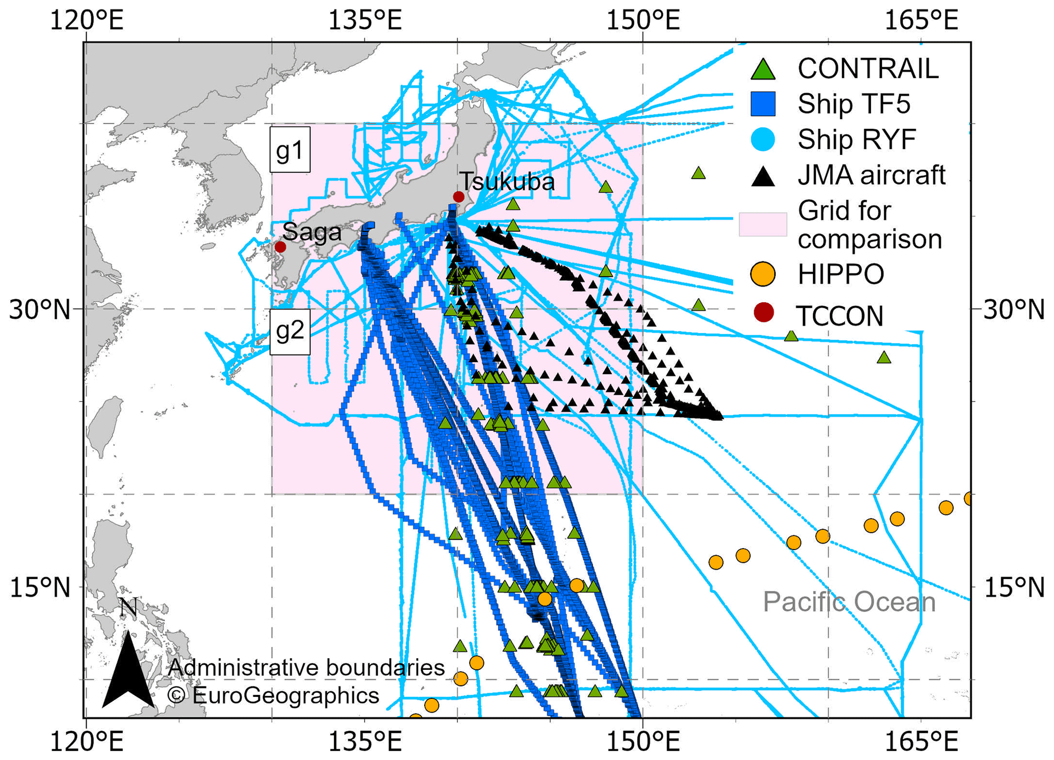
Figure 1 Location of CH₄ in situ data from aircraft (CONTRAIL has black triangles; JMA aircraft have black triangles), ship (ship TF5 has blue squares; ship RYF has light blue circles) between 2014 and 2018. Also shown are the locations of the TCCON stations (red circles) and HIPPO profile flights (yellow circles). Selected regions within 10° × 20° latitude–longitude boxes are shown as pink shaded areas. Map credit: Administrative boundaries © EuroGeographics.

Measurements with the MSE are conducted when the ASE cannot be operated. Sample air is taken from the air outlet nozzle in the cockpit, using a manual diaphragm pump. The sampling method is similar to that used during aircraft observations by the Japan Meteorological Agency (JMA) (Tsuboi et al., 2013; Niwa et al., 2014). Only ASE and MSE data which were obtained below the tropopause height during the cruising part of the flight at around 11 km altitude (∼ 200 hPa) are used. We used the blended tropopause pressure (TROPPB) to define the tropopause height, which is explained in detail in Sect. 2.3. Data of the lower stratosphere were only occasionally obtained and screened out.

Air samples of the mid troposphere at about 6 km altitude (∼ 450 hPa) were collected by a cargo aircraft C-130H between Kanagawa prefecture (35°27^′ N, 139°27^′ E) near Tokyo and Minamitorishima (MNM) (24°17^′ N, 153°59^′ E), which is about 2000 km southeast of Tokyo. The observations were conducted by JMA in cooperation with the Japan Ministry of Defense about twice a month, either by direct flights or via Iwo Jima (24°47^′ N, 141°19^′ E), which is about 1000 km south of Tokyo. Air samples from the air-conditioning system were collected and analyzed at the JMA, using a cavity ring-down spectroscopy (CRDS) analyzer (Picarro Inc., Santa Clara, CA, USA, G2301) (Saito, 2022). The concentrations of CH₄ are determined by the JMA standard gases that are traceable to the WMO standard scales. The reproducibility of CH₄ concentration of different flasks has a precision of ± 0.68 ppb (Tsuboi et al., 2013).

2.2 Ship

Commercial cargo Ships of Opportunity (SOOP) have been collecting air samples since 2001 between Japan and North America, since 2005 between Japan and Australia and New Zealand, and since 2007 between Japan and Southeast Asia. In this study, we used CH₄ observations by the cargo ship Trans Future 5 (TF5; Toyofuji Shipping Co., Ltd.), which sails between Japan, Australia, and New Zealand (Fig. 1). Each round trip takes about 5 weeks (Terao et al., 2011). Concentrations of CH₄ were continuously measured using a CRDS analyzer (Picarro, Inc.; models EnviroSense 3000i and G1202). In parallel, concentrations of CO₂ and O₃ were measured. The same instrumentation and analysis methodology was used and described in detail in Nara et al. (2014). In short, the air intake was placed at the bow on the top of the bridge at about 28 m above sea level, 163 m away from the smokestack at the stern (Terao et al., 2011). Exhaust-contaminated samples were rejected when the dry-air mole fractions of CO₂ and O₃ showed an abrupt increase and decrease, respectively. The analytical precision for 1 min measurements was 0.5 ppb. Calibration with three standard gases was performed for 30 min (10 min for the respective gas) once every 2 d. The standard gases were calibrated against the NIES-94 CH₄ scale.

In addition, atmospheric CH₄ data collected by the research vessel Ryofu Maru (RYF; operated by JMA) on the Pacific Ocean were used (Enyo and Kadono, 2021). The intake for air samples was about 8 m above the sea surface. Air samples were dried, and the mole fraction of CH₄ was determined by gas chromatography (Shimadzu, GC-8A). After 2016, data were collected using off-axis integrated cavity output spectroscopy (Los Gatos Research, GGA-30r). Calibration with three standard gases was performed every hour and every 12 h after 2016.

2.3 Models

The Model for Interdisciplinary Research on Climate, version 4.0 (MIROC4)-based atmospheric chemistry transport model (ACTM) has a horizontal resolution of triangular truncation 42 (T42), which corresponds to approximately 2.8° longitude by 2.8° latitude. Details of the MIROC4-ACTM are described in Patra et al. (2018). The MIROC4-ACTM uses 67 vertical layers between the Earth's surface and 0.0128 hPa. Hybrid vertical coordinates are used to resolve gravity wave propagation in the stratosphere, where at least 30 model layers reside. The ACTMs are nudged with the Japanese 55-year Reanalysis data (JRA-55; Kobayashi et al., 2015) for horizontal winds and temperature at Newtonian relaxation times of 1 and 5 h, respectively. A high accuracy of the MIROC4-ACTM is indicated by the agreement of simulated and observed “age of air”, and the interhemispheric gradient of SF₆ (Patra et al., 2018).

The Copernicus Atmosphere Monitoring Service (CAMS), operated by the European Centre for Medium-Range Weather Forecasts (ECMWF), provides global greenhouse gas reanalysis (EGG4) data. The CAMS reanalysis dataset assimilates satellite observations of atmospheric trace gases and global emission datasets. The horizontal resolution at a spectral truncation of T255 corresponds to a 0.7° × 0.7° (longitude–latitude) grid. The vertical model resolution consists of 60 hybrid sigma-pressure levels, which are interpolated to 25 pressure levels between 1000 and 1 hPa, with about 12 levels in the stratosphere (Inness et al., 2019). In this study, we used EGG4 CH₄ data with monthly average fields (version v20r2) (ECMWF, 2024a). Furthermore, we used the CAMS global inversion-optimized greenhouse gas fluxes and concentrations dataset (CAMSinv) v20r1 (ECMWF, 2024b), which accounts for chemical loss in the troposphere and stratosphere. The inversion-optimized dataset has a horizontal resolution of a 2° × 3° (longitude–latitude) grid and 34 pressure levels between 1001 and 0.5 hPa (Segers and Steinke, 2022). We choose datasets which assimilate NOAA surface observations but not GOSAT observations to ensure that the model results in our approach are independent from the satellite we aim to validate.

Furthermore, we extracted data of the TROPPB, which is defined as a combination of a thermal tropopause and dynamic tropopause pressure (Wilcox et al., 2012). The TROPPB data are extracted from GEOS-FP-IT (Goddard Earth Observing System–Forward Processing for Instrument Teams; GES-DISC, 2022) meteorology data using the Python suite ginput, version 1.0.6 (Laughner et al., 2023). At 10° × 20° latitude–longitude boxes (Sect. 3.1), the TROPPB was calculated daily every 3 h for the center and the four corner locations and was then monthly averaged.

2.4 Satellite

Japan's GOSAT, launched in 2009, was developed to characterize the variability in the atmospheric CO₂ and CH₄ fractions at regional scales over the globe. The TANSO-FTS instrument on board GOSAT measures the reflected sunlight in three SWIR channels: centered at 0.764 µm (Band 1), at 1.61 µm (Band 2), and at 2.06 µm (Band 3) (Kuze et al., 2009). XCH₄ is estimated by taking the ratio of the total column amounts of CH₄ and the total column of dry air, which are extending from the Earth's surface to the top of the atmosphere.

The methodology to derive XCH₄ depends on the retrieval algorithm. For the NIES retrieval, profiles of the dry-air partial columns of CO₂, CH₄, O₂, and water vapor (H₂O) were simultaneously retrieved, based on the maximum a posteriori (MAP) retrieval (Rodgers, 2000; Yoshida et al., 2013). The total column of dry air is primarily derived from the surface pressure in consideration of the retrieved H₂O profile and meteorological profiles from JMA (Yoshida et al., 2011, 2013). In case of the RemoTeC full-physics retrieval, operated at the Netherlands Institute for Space Research (SRON), the European Space Agency (ESA), and at Heidelberg University, Germany, the dry-air column is calculated from ECMWF meteorological data (Butz et al., 2011). Another full-physics retrieval of the University of Leicester is based on the original Orbiting Carbon Observatory (OCO) retrieval and was modified for use with GOSAT spectra (UoL-OCFP) (Boesch and Noia, 2023). Furthermore, NIES, RemoTeC, and UoL-OCFP differ in the number of vertical layers and the aerosol parameterization, which includes the number of aerosol types (Yoshida et al., 2013; Butz et al., 2011; Guerlet et al., 2013; Takagi et al., 2014; Boesch and Noia, 2023).

In this study, we selected level 2 XCH₄ data in sunglint mode from the NIES v02.95 (GDAS, 2023), the RemoTeC v2.3.8 full-physics retrieval from SRON, and the UoL-OCFP v7.3 (Copernicus Climate Change Service, Climate Data Store, 2018). A comparison with the RemoTeC v2.4.0 full-physics retrieval operated at Heidelberg University is shown in Appendix A (Fig. A4). All data were bias-corrected and cloud-screened using the cloud flags obtained from the TANSO-CAI (Cloud and Aerosol Imager) on board GOSAT (Yoshida et al., 2011, 2013; Butz et al., 2011). In the following, we refer to data obtained by the retrieval algorithm from NIES v02.95, RemoTeC v2.3.8, and UoL-OCFP v7.3 simply as NIES, RemoTeC, and OCFP, respectively. The comparison with XCH₄ data retrieved from other satellites like GOSAT 2, launched in 2018, and TROPOMI, launched at the end of 2017, was not possible in our study, due to missing aircraft data after mid-2017 (Sect. 2.1).

3 Methodology

3.1 Study region

Figure 1 shows the study region and location of CH₄ in situ data. All data obtained over land are excluded. We selected the latitude–longitude ranges, where g1 is 30–40° N, 130–150° E, and g2 is 20–30° N, 130–150° E in the western Pacific for the years from 2014 to the end of 2017 for two reasons. First, we want to use the same years and region where we successfully derived the ship–aircraft-based column-averaged dry-air mole fraction of CO₂ previously (Müller et al., 2021). To obtain enough co-located data for the seasonal and interannual comparison with satellite retrievals, 10° × 20° latitude–longitude boxes were chosen, where g1 is expected to be more strongly influenced by the emission outflow from land as compared to g2 (Fig. 1). Second, the temporal and spatial coincident ship and aircraft CH₄ data are currently limited to the northern west Pacific until mid-2017 (Sect. 2.1). Within the two latitude–longitude boxes, we calculate monthly averages of the satellite and in situ observations and model results. The average number of monthly satellite observations at g1 and g2 for NIES is 28 ± 13 (24 months) and 34 ± 24 (31 months); for RemoTeC is 24 ± 16 (11 months) and 41 ± 24 (24 months); and for OCFP is 8 ± 2 (6 months) and 14 ± 11 (27 months), respectively. Months with fewer than five observations are excluded. Ship observations of TF5 and RYF from the south and east of Japan were combined. On average, we obtained 6 ± 4 d of ship observations each month. The number of monthly aircraft observations was 2 ± 1 for both latitude ranges. In our study, we develop the methodology for the future application with higher numbers of in situ data.

3.2 Observation-based CH₄ profile construction and XCH₄ calculation

Figure 2 illustrates the principle of how to construct ship–aircraft-based CH₄ profiles from which XCH₄ is derived. Ship data are extrapolated vertically up to ∼ 850 hPa, which represents the pressure level of the boundary layer above sea level. During boreal summer, a higher OH concentration contributes to an increased CH₄ removal by oxidation at our study region (Travis et al., 2020). Including other atmospheric factors, such as the atmospheric circulation pattern, models estimate the instantaneous lifetime of CH₄ for July to be as short as 1 year (Fig. 14 in Patra et al., 2009). In the same period, the CH₄ concentration can be increased in the mid to upper troposphere at the western Pacific by CH₄-rich air masses transported from South and East Asia (Umezawa et al., 2012). To constrain the tropospheric CH₄ variability, CONTRAIL aircraft data from the cruise portion of the flight at around 200 hPa and JMA aircraft data from about 450 hPa are selected, which represents the upper and middle troposphere, respectively.

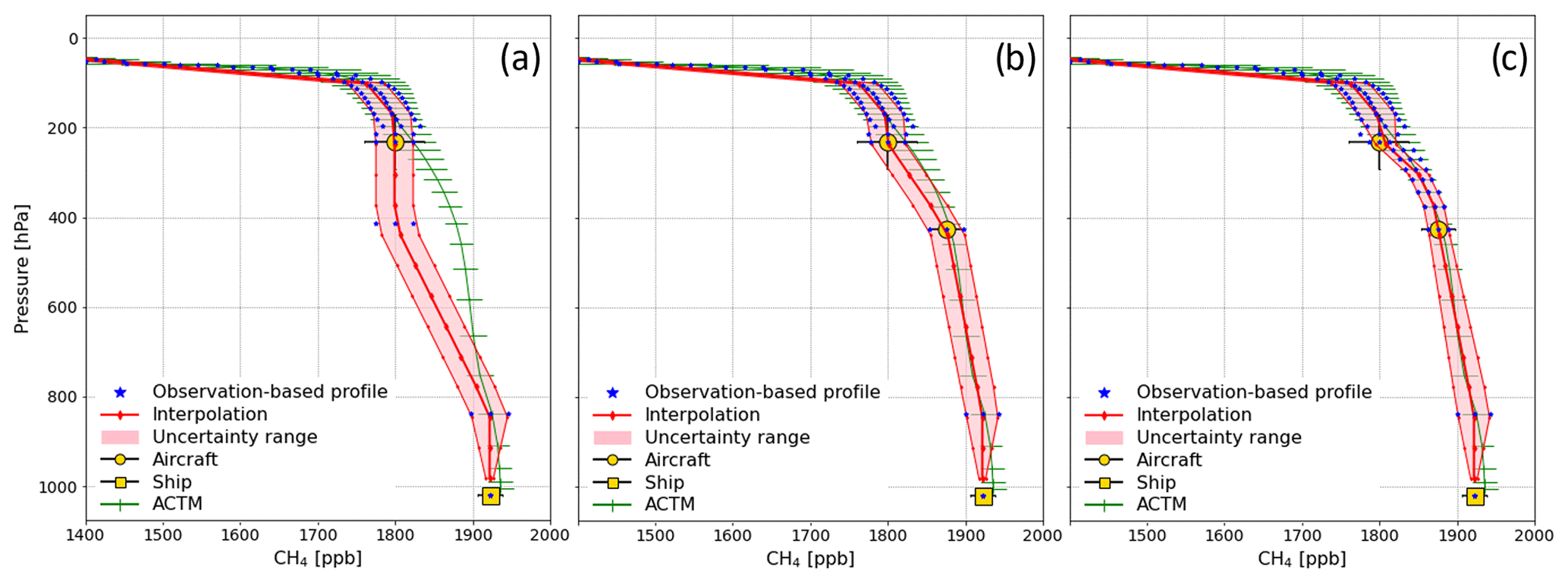
Figure 2 Construction of the observation-based CH₄ profile (blue) obtained by using ship and aircraft data (yellow), together with model results (green) and the interpolation onto the pressure grid of the satellite retrieval (red) for approach 1 (a), approach 2 (b), and approach 3 (c). The example is obtained at the latitude 30–40° N, in March 2015.

In the following, we test three approaches. Approach 1 is the adaptation of the approach of Müller et al. (2021) (Fig. 2a). We extrapolate CONTRAIL data upwards to the TROPPB and downwards to the lower cruising height at 400 hPa without the constraint of the JMA aircraft data. Then we linearly interpolate in both the pressure and dry-air mole fraction between the extrapolated ship data and the extrapolated aircraft data. Approach 2 is the addition of JMA aircraft data to the mid troposphere (Fig. 2b). We linearly interpolate between the extrapolated ship data and both aircraft data. In approach 3, we fill in model results between the aircraft data of JMA and CONTRAIL of approach 2 (Fig. 2c). Since CONTRAIL flies very close to the TROPPB, we do not fill model data between CONTRAIL and the TROPPB. Above the TROPPB, we use model results in all three approaches. To calculate the XCH₄ that the satellite would have seen, given our constructed CH₄ profile, we first interpolate these profiles onto the corresponding monthly averaged pressure grid of the satellite retrievals, and then we use Eq. (15) of Connor et al. (2008):

$$\begin{array}{}\text{(1)}& X_{{\mathrm{CH}}_{\mathrm{4}}}^{\mathrm{m}}=X_{{\mathrm{CH}}_{\mathrm{4}}}^{\mathrm{a}}+\sum _j{h}_j{a}_{{\mathrm{CH}}_{\mathrm{4}},j}(x_{\mathrm{m}}-x_{\mathrm{a}}{)}_j,\end{array}$$

where $X_{{\mathrm{CH}}_{\mathrm{4}}}^{\mathrm{m}}$ is the XCH₄ which the satellite would report if it observed the constructed CH₄ profile x_m (as a true profile). Extracted from the satellite retrievals, $X_{{\mathrm{CH}}_{\mathrm{4}}}^{\mathrm{a}}$ is the a priori XCH₄, h_j the pressure weighting function, $a_{{\mathrm{CH}}_{\mathrm{4}},j}$ the column averaging kernel, and x_a the a priori CH₄ profile. In this study, we use only the pressure grid and parameters of NIES. In the following, we refer to the calculated $X_{{\mathrm{CH}}_{\mathrm{4}}}^{\mathrm{m}}$ as simple observation-based XCH₄ (simple obs. XCH₄), observation-based XCH₄ (obs. XCH₄), and model-blended observation-based XCH₄ (blended obs. XCH₄) for results of approach 1, 2, and 3, respectively.

3.3 Uncertainty assessment of obs. CH₄ profiles

There are two uncertainty sources. The first uncertainty source arises from the limited number and spatiotemporal distribution of in situ data within the latitude–longitude boxes of each month. Therefore, the data may not always represent the monthly averaged CH₄ concentration within the area of interest accurately. However, in the near future, the number of in situ data points will increase, and the spatial distribution will expand, as discussed in Sect. 5. The second source of uncertainties in the obs. XCH₄ (simple and blended) are caused by the CH₄ profile construction as follows: (a) the inter- and extrapolation of the in situ data in the troposphere, (b) the tropopause height, and (c) the modeled stratospheric column.

3.3.1 Tropospheric uncertainty

First, to assess the uncertainty due to the inter- and extrapolation, we investigated the variability in the CH₄ dry-air mole fractions observed by profile flights of the HIPPO number 4 campaign (HIPPO 4) over the Pacific Ocean (Wofsy, 2011). Between 14 June and 11 July 2011, 20 profiles ranging from the surface up to about 13 km were obtained near the study region (Fig. 1). Within each profile, the CH₄ dry-air mole fractions show variations between 9 and 62 ppb (24 ± 17 ppb; Table 1). The highest range was seen in the middle to upper troposphere during these summer months, consistent with observations by Umezawa et al. (2012). Based on this variation, we use 24 ppb uncertainty between the extrapolated ship data and the TROPPB for the profile construction in approach 1.

Table 1 Uncertainty assessment of the obs. CH₄ profiles at the troposphere. Top rows show the average concentration range of CH₄ within each HIPPO 4 profile (mean variability ± standard deviation). Bottom rows show the root mean square error (RMSE) of the difference between MIROC4-ACTM (ACTM) and HIPPO 4 and MIROC4-ACTM and obs. CH₄ profile data at different altitude ranges. The last column shows the total uncertainty after Gaussian error propagation. Uncertainties applied to approach 3 are shown in bold.

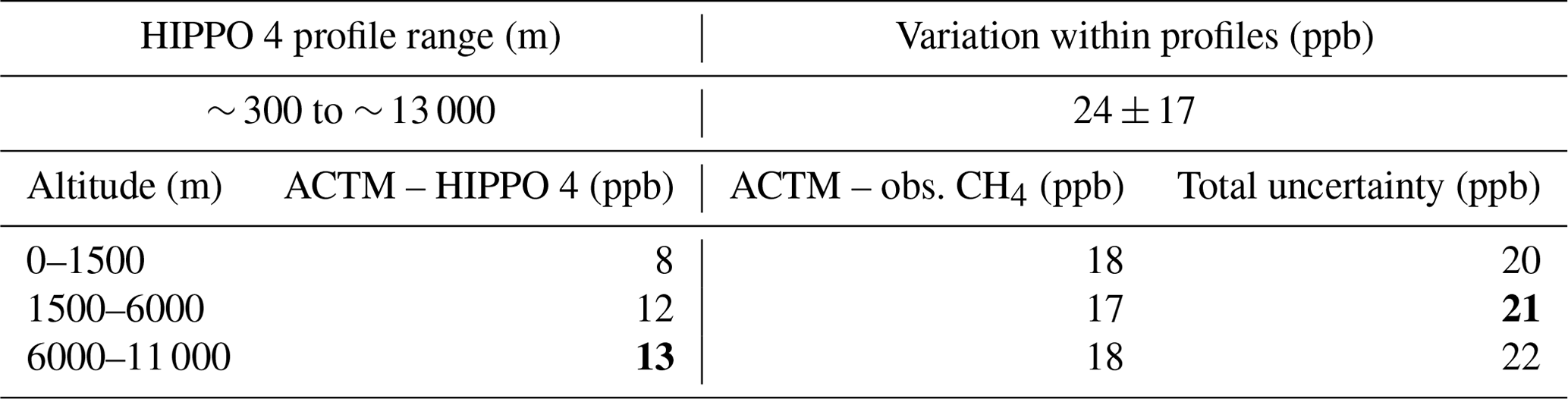
Second, we assessed the uncertainty in the constructed CH₄ profiles in three steps with the help of the MIROC4-ACTM. In the first step, we investigate how well the MIROC4-ACTM reproduces the variation in HIPPO profiles for similar conditions to our study region, which is influenced by the continental emission outflow (Appendix A; Fig. A1). Therefore, we selected eight profiles within 2000 km of the center location of g2 (Fig. 1). The MIROC4-ACTM was chosen to be consistent with our previous study. (Müller et al., 2021). We distinguished the altitude range 0–1500 m, corresponding to the boundary layer, 1500–6000 m, which corresponds to the middle troposphere between the extrapolated ship and JMA aircraft data, and 6000–11000 m, which corresponds to the upper troposphere between the JMA and CONTRAIL aircraft data. As model uncertainty, we obtain the root mean square error (RMSE) of the difference between the MIROC4-ACTM and the HIPPO profiles with 8, 12, and 13 ppb for the altitude ranges 0–1500, 1500–6000, and 6000–11 000 m, respectively (Table 1). In the second step, we compare the MIROC4-ACTM with our obs. CH₄ profiles and obtain the RMSE (Table 1; ACTM – obs. CH₄). Because the model itself has an uncertainty, as obtained in step 1, the tropospheric uncertainty in the constructed profile of each altitude range is 20, 21, and 22 ppb using Gaussian error propagation (Table 1; Total uncertainty column). As a result, we added 21 ppb uncertainty between the extrapolated ship and JMA data in approaches 2 and 3 and 22 and 13 ppb between the JMA data and up to the TROPPB in approaches 2 and 3, respectively.

3.3.2 Tropopause uncertainty

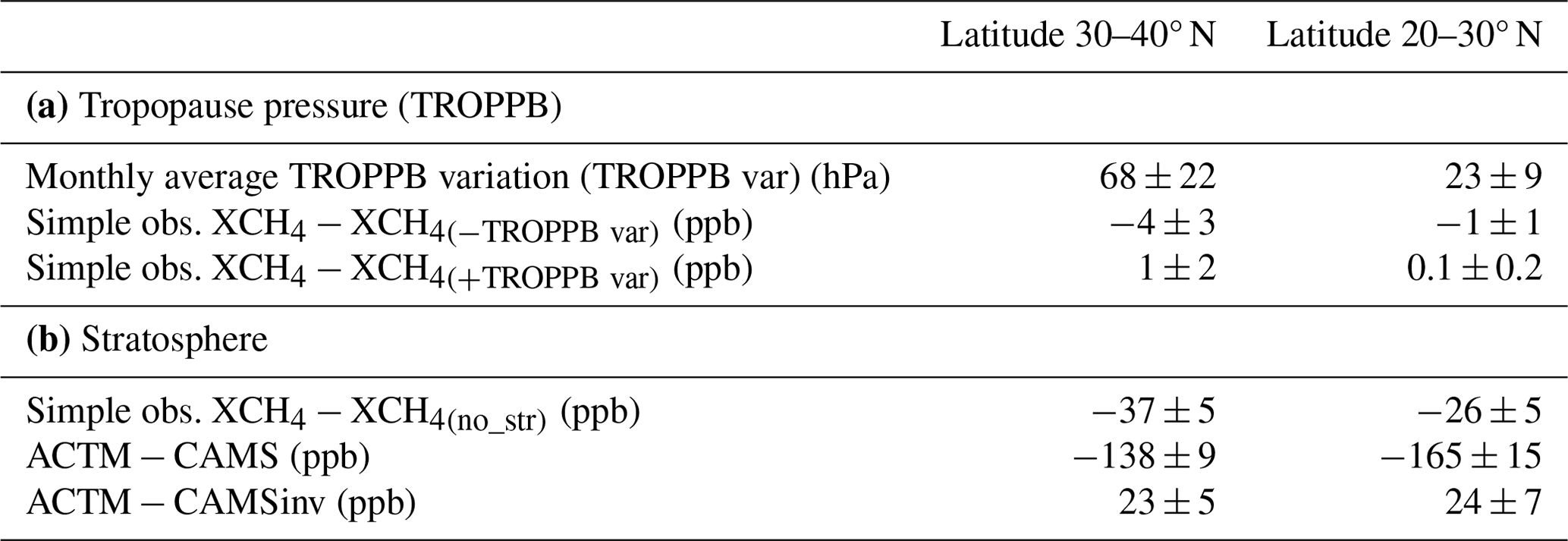
The variation in the monthly averaged TROPPB (Sect. 2.3) at 30–40° N was more than twice that at 20–30° N with an average standard deviation of 68 ± 22 and 23 ± 9 hPa, respectively (Table 2). The maximum difference of 90 hPa (68 + 22 hPa) and 32 hPa (23 + 9 hPa) at the level of the TROPPB corresponds to an altitude difference of 3–4 and 1–2 km, respectively. To test the impact of the TROPPB on the derived XCH₄, we first calculated the simple obs. XCH₄. Second, we calculated the simple obs. XCH₄ with TROPPB ± 90 hPa at 30–40° N and TROPPB ± 32 hPa at 20–30° N, based on the monthly averaged variability in the TROPPB. Then, we compared the latter two results with the original simple obs. XCH₄. The average difference in the resulting XCH₄ at 30–40 and 20–30° N for the reduced TROPPB (−90 and −32 hPa) was −4 ± 3 and −1 ± 1 ppb, respectively. If the TROPPB was increased (+90 and +32 hPa), then the difference was small as 1 ± 2 and 0.1 ± 0.2 ppb (Table 2). Because model results are used above the TROPPB, a TROPPB that is too high (an altitude that is too low) can be compensated by the model. In total, the TROPPB causes an uncertainty of less than 0.4 % on the calculated XCH₄.

Table 2 (a) Uncertainty at the blended tropospause pressure (TROPPB) by calculating the difference between simple obs. XCH₄ and the sum of the simple obs. XCH₄ and reduced/increased TROPPB (XCH_{4(± TROPPB  var)}) (mean difference ± standard deviation of differences). TROPPB var is the monthly average variability in TROPPB (mean standard deviation of the monthly averages ± standard deviation). (b) Uncertainty at the stratospheric column by calculating the difference between simple obs. XCH₄ and simple obs. XCH₄ with extrapolated aircraft data up to 0.0128 hPa (XCH_{4(no_str)}) and the differences between the modeled stratosphere of MIROC4-ACTM (ACTM) and CAMS, and ACTM and CAMSinv (mean difference ± standard deviation of differences).

3.3.3 Stratospheric uncertainty

CH₄ shows variations in the stratosphere due to its reactions with excited oxygen (O(¹D)), OH, and chlorine radicals (Saunois et al., 2020), which is represented in each model differently. GOSAT NIES CH₄ observations have a higher sensitivity in the stratospheric column, as compared to CO₂ (averaging kernel > 0.8 in the stratosphere; Appendix A; Fig. A2). Therefore, the shape and value of the modeled stratospheric CH₄ column impact the derived column-averaged dry-air mole fractions more than those for CO₂.

In the first step, we used the simple obs. XCH₄ to test the sensitivity of the stratospheric column on the derived XCH₄. We extrapolated CONTRAIL aircraft data through the TROPPB and the stratosphere up to 0.0128 hPa. XCH₄ calculated from profiles without considering the stratosphere was higher than the simple obs. XCH₄ by 37 ± 5 ppb (2.0 ± 0.3 %) and 26 ± 5 ppb (1.4 ± 0.3 %) at 30–40 and 20–30° N, respectively (Table 2), which confirms the importance of the stratospheric column to derive XCH₄ correctly.

In the second step, we assessed the uncertainty in the stratospheric model. We calculated the difference MIROC4-ACTM − CAMS and MIROC4-ACTM − CAMSinv of the monthly averaged data above the TROPPB. For that, we interpolated the MIROC4-ACTM data with its higher resolved pressure grid on that of the CAMS and CAMSinv data, respectively (Sect. 2.3). CAMS was positively biased by 138 ± 9 and 165 ± 15 ppb at 30–40 and 20–30° N, respectively (Table 2; Appendix A; Fig. A3a and b). In contrast, the total average difference between MIROC4-ACTM and CAMSinv was small as 23 ± 5 and 24 ± 7 ppb at 30–40 and 20–30° N, respectively. In addition, the difference MIROC4-ACTM − CAMSinv depends on the season. The highest average difference occurred in June (30–40° N, with 37 ± 6 ppb; 20–30° N, with 44 ± 3 ppb) and the lowest in October (4 ± 0.6 ppb) at 30–40° N, January (5 ± 5 ppb), and February (3 ± 13 ppb) at 20–30° N (Appendix A; Fig. A3c and d). A large positive stratospheric CH₄ bias of around 200 ppb of CAMS was recently reported by Agustí-Panareda et al. (2023), consistent with our observations. They suggest that uncertainties associated with the stratospheric chemical loss of CH₄ are the largest contributor to that bias. Compared to CAMS, both the MIROC4-ACTM and CAMSinv account for chemical losses in the stratosphere. Additionally, MIROC4-ACTM uses an optimized atmospheric transport model (Patra et al., 2018). The seasonality of the difference in MIROC4-ACTM − CAMSinv indicates that the seasonally dependent chemical loss of CH₄ and/or meridional transport processes are modeled differently in both models.

Based on the total average difference between the latter two models, we added a ± 24 ppb uncertainty to the stratospheric column of the constructed CH₄ profile. The impact of the three stratospheric models on the calculated XCH₄ using this uncertainty is discussed in Sect. 4.2.

4 Results and discussion

4.1 Evaluation of the approaches

Figure 3 shows the temporal variation in the XCH₄ calculated for the two selected latitude ranges (g1 is 30–40° N; g2 is 20–30° N) using approach 1 (simple obs. XCH₄), approach 2 (obs. XCH₄), and approach 3 (blended obs. XCH₄). For the period 2014 to mid-2017, we obtained 20 and 31 monthly averaged XCH₄ at the latitude ranges 30–40 and 20–30° N, respectively. The uncertainty range of the simple obs. XCH₄ (22 ppb) is 2 and 6 ppb larger than those of the obs. XCH₄ (20 ppb) and blended obs. XCH₄ (16 ppb), respectively (Sect. 3.3). Furthermore, the difference between the latter two approaches is as small as 1 ± 3 ppb (blended obs. XCH₄ − obs. XCH₄) at both latitude ranges. In contrast, the difference between simple and blended obs. XCH₄ shows a variability of 2 ± 11 and 4 ± 9 ppb at 30–40 and 20–30° N, respectively.

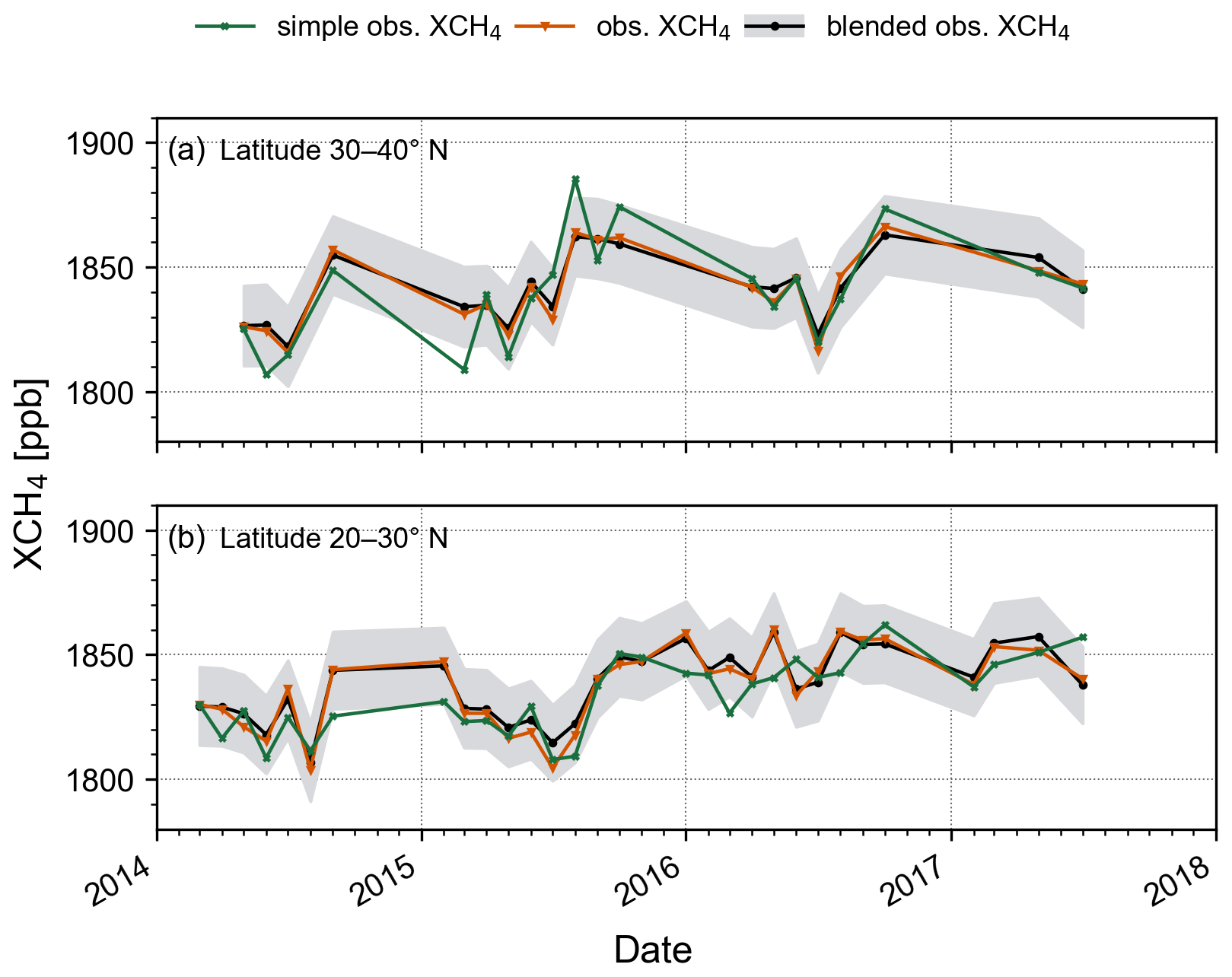
Figure 3 Temporal variation in the monthly averaged XCH₄ obtained by approach 1 (simple obs. XCH₄; green), approach 2 (obs. XCH₄; orange), and approach 3 (blended obs. XCH₄; black) at the latitude ranges 30–40° N (a) and 20–30° N (b). The uncertainty ranges are 22, 20, and 16 ppb for approaches 1, 2, and 3, respectively. Only the 16 ppb uncertainty range of approach 3 is shown as gray area. Other uncertainty ranges are omitted for readability.

To assess the correctness of the XCH₄ datasets, we compare our data at both latitude ranges with the monthly averaged XCH₄ data (version GGG2020) obtained from the nearest ground-based TCCON stations in Tsukuba (36.05° N, 140.12° E; Morino et al., 2022) and Saga (33.24° N, 130.29° E; Shiomi et al., 2022) (Figs. 1 and 4). Compared to Tsukuba, Saga is influenced by the continental outflow of air masses from East Asia. It is noted that the distance of about 1300 km between the TCCON stations and the center of g2 is large. Considering that there are no strong CH₄ sources over the open ocean at g2, the comparison gives us an indication about the applicability of the datasets.

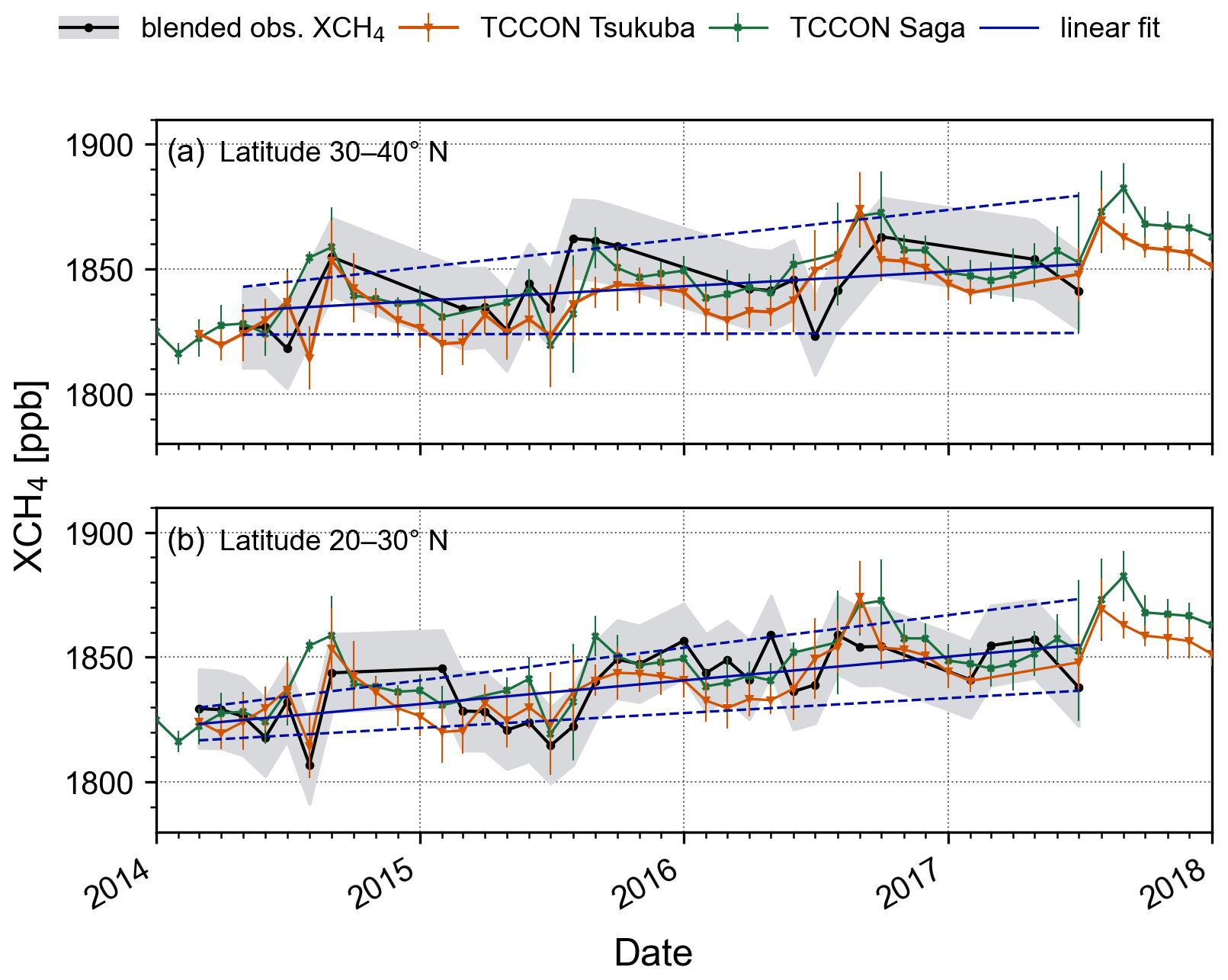
Figure 4 Temporal variation in the monthly averaged XCH₄ obtained by approach 3 (blended obs. XCH₄; black) and from the TCCON station in Saga (green) and Tsukuba (orange) at the latitude ranges 30–40° N (a) and 20–30° N (b). The gray area is the 16 ppb uncertainty range of approach 3; error bars are the standard deviations of TCCON. Also shown is the linear least square regression (deep blue line), with a 90 % confidence interval on the slope and intercept (dashed deep blue line) of approach 3.

For readability, only the blended obs. XCH₄ in comparison with the TCCON stations is shown in Fig. 4. By looking at the averaged difference at g1, XCH₄ from Tsukuba was lower than that derived from our approaches with −3 ± 20, −3 ± 14 and −4 ± 13 ppb for approaches 1, 2, and 3, respectively. In contrast, XCH₄ from Saga was higher and showed better agreement with differences of 1 ± 20 ppb for approach 1 and 1 ± 12 ppb for approaches 2 and 3. At g2, XCH₄ from Tsukuba matches our data better than that from Saga with 3 ± 11, 0 ± 12, and −1 ± 11 ppb for approaches 1, 2, and 3. Saga showed a higher discrepancy of 9 ± 12, 6 ± 14, and 5 ± 14 ppb for the respective approaches. The similarity between XCH₄ from our approaches and Saga at g1, and Tsukuba at g2, indicates that the ocean area at 30–40° N (g1) is rather influenced by the continental outflow of CH₄ from Asia, while 20–30° N (g2) showed cleaner conditions.

Given the lower maximal possible averaged difference between TCCON and approaches 2 and 3 compared to approach 1, and given the lowest uncertainty range of approach 3, the latter approach is preferable for future applications. Therefore, we use the results of approach 3 (blended obs. XCH₄) for further discussion.

4.2 Evaluation of the stratospheric model

Figure 5 shows the comparison of the blended obs. XCH₄ (approach 3) using the MIROC4-ACTM, CAMS, and CAMSinv for the stratospheric column (Sect. 3.3.3), denoted as ${\mathrm{ACTM}}_{{\mathrm{XCH}}_{\mathrm{4}}}$, ${\mathrm{CAMS}}_{{\mathrm{XCH}}_{\mathrm{4}}}$, and ${\mathrm{CAMSinv}}_{{\mathrm{XCH}}_{\mathrm{4}}}$. Using ${\mathrm{ACTM}}_{{\mathrm{XCH}}_{\mathrm{4}}}$ as reference, ${\mathrm{CAMS}}_{{\mathrm{XCH}}_{\mathrm{4}}}$ is highly biased at both latitude ranges by 12 ± 5 ppb (0.6 ± 0.2 %) in total. In contrast, ${\mathrm{CAMSinv}}_{{\mathrm{XCH}}_{\mathrm{4}}}$ shows a small negative total bias of −5 ± 3 ppb (−0.3 ± 0.2 %). CAMS has a known large positive stratospheric CH₄ bias (Agustí-Panareda et al., 2023). MIROC4-ACTM and CAMSinv account for stratospheric CH₄ loss and the modeled stratosphere is comparable as discussed in Sect. 3.3.3. The similarity of the ${\mathrm{ACTM}}_{{\mathrm{XCH}}_{\mathrm{4}}}$ and ${\mathrm{CAMSinv}}_{{\mathrm{XCH}}_{\mathrm{4}}}$ and their differences to ${\mathrm{CAMS}}_{{\mathrm{XCH}}_{\mathrm{4}}}$ indicate the strong impact of the stratospheric part on the derived XCH₄ and highlight the importance of making an appropriate model choice (compare Sect. 3.3.3). Considering the large uncertainty in the CAMS and the fact that the other two products are better optimized for modeling CH₄ in the stratosphere, we suggest using either the MIROC4-ACTM or CAMSinv to model the stratospheric column. In the following, we use the ${\mathrm{ACTM}}_{{\mathrm{XCH}}_{\mathrm{4}}}$ to demonstrate the applicability of the dataset for satellite evaluation. However, for the operational application in future, the publicly available CAMSinv might be the better choice until the MIROC4-ACTM will be available in near-real time.

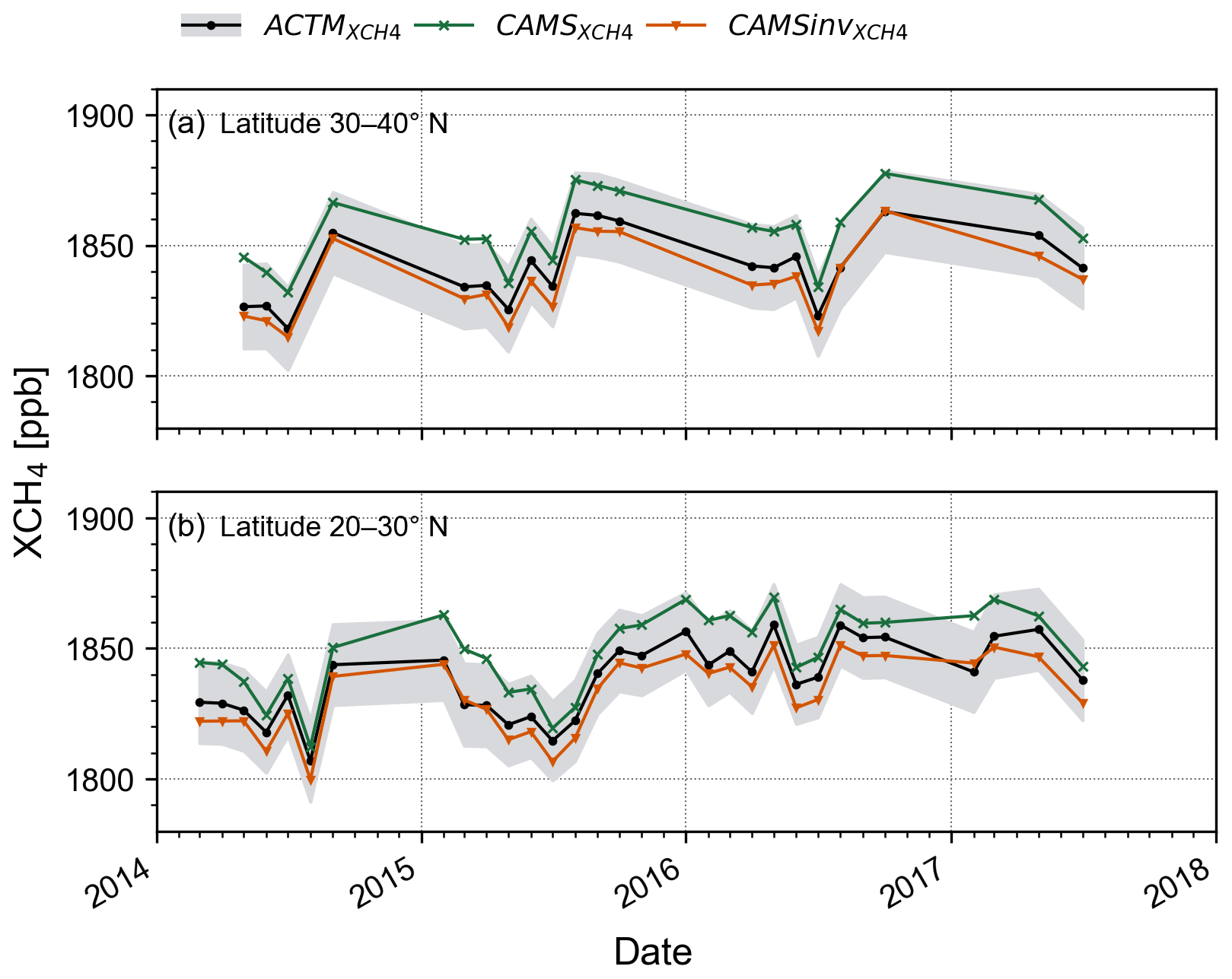
Figure 5 Comparison between the blended obs. XCH₄ (approach 3) derived from CH₄ profiles using the MIROC4-ACTM (${\mathrm{ACTM}}_{{\mathrm{XCH}}_{\mathrm{4}}}$; black), CAMS (${\mathrm{CAMS}}_{{\mathrm{XCH}}_{\mathrm{4}}}$; green), and CAMSinv (${\mathrm{CAMSinv}}_{{\mathrm{XCH}}_{\mathrm{4}}}$; orange) for the stratospheric column at the latitude ranges 30–40° N (a) and 20–30° N (b). The uncertainty range of all results is 16 ppb. The gray area is the uncertainty in ${\mathrm{ACTM}}_{{\mathrm{XCH}}_{\mathrm{4}}}$. Uncertainty ranges of the other results are not shown for readability.

4.3 Applicability of observation-based XCH₄

In the following, we want to demonstrate the applicability of the in situ derived XCH₄ datasets for carbon cycles studies by analyzing the seasonal variation in XCH₄ over the ocean and for the satellite evaluation. We will focus on the blended obs. XCH₄.

4.3.1 Seasonal variation

Figure 3 shows that all three approaches follow similar temporal variations and trends. At 30–40° N, a rough seasonal cycle with lower values between winter and summer (minima in July) and maxima between August to October is seen. The column observations of CH₄ are consistent with northern hemispheric surface observations (e.g., Dlugokencky et al., 1995). Minima between July and August and maxima in the period winter to spring have been observed at the lower troposphere by aircraft and ground-based stations in Japan (Umezawa et al., 2014; Tohjima et al., 2002). The seasonal characteristics are explained by the interaction between air mass origin and atmospheric OH concentration. In summer, southeasterly air masses from CH₄ source-free regions of the Pacific Ocean and the surrounding of Japan are dominant. In addition, the OH concentration is highest in summer, which leads to enhanced CH₄ removal from the atmosphere. In winter, when the removal through OH oxidation is lowest, prevailing northwesterly winds bring CH₄ rich air masses from China and Siberia (Umezawa et al., 2014; Tohjima et al., 2002). This explains the larger CH₄ concentration during that period.

At 20–30° N, lower values are obvious from winter to the end of summer (August) in 2015, but in 2016, it is not as clear as at 30–40° N. Figure 4 also shows the linear least squares regression, with 90 % confidence interval on the slope and intercept of approach 3. At 30–40° N, the annual increase in XCH₄ is within the uncertainty range, with 9 ± 9 ppb for the simple obs. XCH₄ and 6 ± 6 ppb for the other two approaches. In contrast, at 20–30° N, the annual increase is significant, with 11 ± 3 ppb for the simple obs. XCH₄ and 10 ± 4 and 9 ± 4 ppb for the obs. and blended obs. XCH₄. The higher summertime values in 2016 contribute to the difference in the growth rates at 20–30° N. Similar strong growth rates have been reported for the global atmospheric CH₄ concentration between 2014 and 2017, with a peak in 2014 of 13 ppb and a minimum in 2016 of 7 ppb (Nisbet et al., 2019). It is noted that limited and uneven sampled in situ data during each month might cause an artificial difference in the growth rates between the latitude ranges. However, given a lower growth rate at the higher-latitude range combined with a higher similarity of the blended obs. XCH₄ with those XCH₄ influenced by the Asian emission outflow at Saga (Chap. 4.1), we can suggest that the interaction between anthropogenic emissions might have led to increased OH concentrations, with higher CH₄ removal rates near to the Japanese east coast (Fig. 1) as a consequence, and therefore caused a slower annual growth. Or it might indicate that compared to 20–30° N, the higher-latitude range is affected by the decreasing trend in CH₄ emissions from Japan (Ito et al., 2023).

A possible explanation for the observed increased summertime XCH₄ values in 2016 can be the characteristics of the prevailing southerly winds in that season. In the years 2015 to 2016, a strong El Niño event of the El Niño–Southern Oscillation (ENSO) took place, which is linked to extreme heat and drought, and consequently to increased biomass burning in tropical regions took place, which is linked to extreme heat and drought, and consequently to increased biomass burning in tropical regions (Bousquet et al., 2006; Parker et al., 2016; Whitburn et al., 2016). Smoldering combustion in peatland fires can release large amounts of CH₄ (Bousquet et al., 2006; Parker et al., 2016). Using GOSAT observations, Parker et al. (2016) reported an enhancement of XCH₄ of 35 ppb above background conditions over Indonesian peatland fires at the end of 2015. Furthermore, Zhang et al. (2018) demonstrated that enhanced CH₄ emissions from wetland areas from January through May 2016 are related to the strong El Niño, which provides an explanation for a rise in the atmospheric CH₄ growth rate. Therefore, southerly air masses of high CH₄ concentration might have affected the study region. Our observations demonstrate the capability of the ship–aircraft-based dataset to capture seasonal variations and climatological events like the El Niño.

4.3.2 Satellite evaluation

Figure 6 shows the temporal variation in the blended obs. XCH₄ (${\mathrm{ACTM}}_{{\mathrm{XCH}}_{\mathrm{4}}}$) in comparison with XCH₄ from GOSAT observations using the NIES, RemoTeC, and OCFP retrieval (Sect. 2.4). The retrievals mostly lie in the uncertainty range (16 ppb) of the blended obs. XCH₄. The difference in blended obs. XCH₄ − NIES is −0.04 ± 12.65 and −0.04 ± 13.32 ppb at 30–40 and 20–30° N, respectively. The high standard deviations are similar to that reported for the difference between NIES and TCCON ocean data in the data release note of the NIES GOSAT project (NIES GOSAT Project, 2020). The difference between blended obs. XCH₄ and RemoTeC shows a larger average discrepancy of 11.8 ± 16.2 and 12.1 ± 8.1 ppb but with a smaller standard deviation at 20–30° N. At 30–40° N, OCFP provides almost no valid data. The difference is 2.2 ± 21.0 ppb. At 20–30° N, the difference in blended obs. XCH₄ − OCFP of 10.3 ± 9.6 ppb is similar to the difference in RemoTeC. The smaller standard deviations of RemoTeC and OCFP suggest rather a systematic offset at that latitude range. The higher difference compared to NIES can arise from the choice of a priori profiles and column averaging kernel in the retrieval and their choice in calculation of the blended obs. XCH₄ (Sect. 3.2). To clarify if the offset of RemoTeC and OCFP is a true regional or ocean bias, further analyses are needed in future.

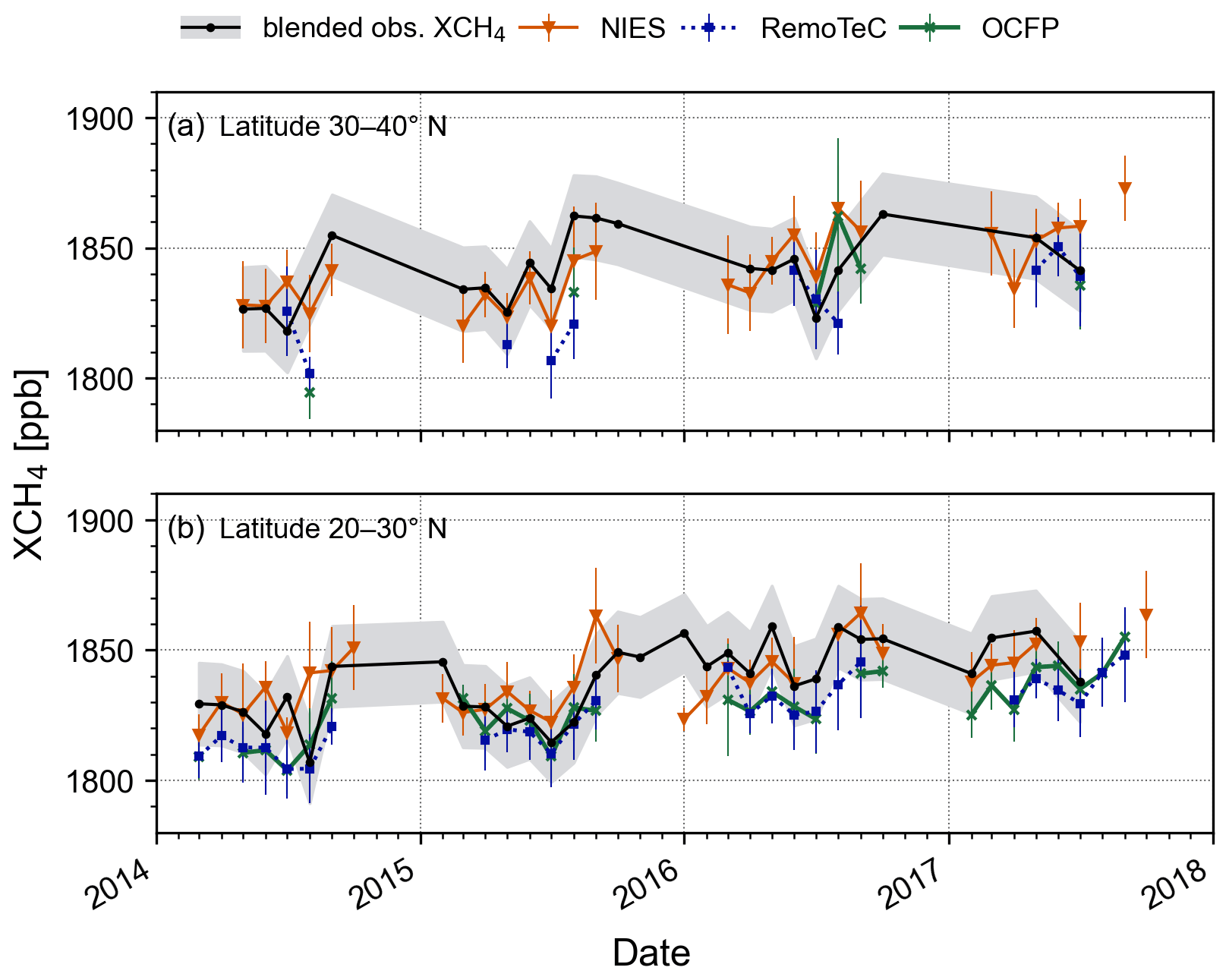
Figure 6 Temporal variation in the blended obs. XCH₄ (${\mathrm{ACTM}}_{{\mathrm{XCH}}_{\mathrm{4}}}$, black) in comparison with GOSAT XCH₄ retrievals from NIES (orange), RemoTeC (blue), and OCFP (green) at the latitude ranges 30–40° N (a) and 20–30° N (b). The gray area is the 16 ppb uncertainty in the blended obs. XCH₄.

5 Summary and conclusion

As a reference dataset for satellite validation and carbon cycle studies, we investigated three different approaches to derive column-averaged dry-air mole fractions of CH₄ (XCH₄) over oceans by integrating commercial ship and aircraft observations. The study focused on the latitude ranges 30–40 and 20–30° N at the longitude 130–150° E between the years 2014 and 2018. Approach 1 used simple linear inter- and extrapolation between ship and aircraft data of the upper troposphere, approach 2 used additional aircraft data of the middle troposphere, and approach 3 added model results between the middle and upper tropospheric aircraft observations. All three approaches used model results for the stratospheric column.

Uncertainties in the calculated XCH₄ were reduced by 2 and 6 ppb from 22 ppb (approach 1) to 20 ppb for approach 2 and 16 ppb for approach 3. XCH₄ derived from approaches 2 and 3 were similar within 1 ± 3 ppb. The difference between approaches 3 and 1 was about 30 % higher. At 30–40° N, XCH₄ data of the TCCON station Saga, influenced by the Asian continental outflow, showed a better agreement with our approaches (within 1 ± 20 ppb for approach 1; 1 ± 12 ppb for approaches 2 and 3) than that from Tsukuba (which was lower by −3 ± 20, −3 ± 14, and −4 ± 13 ppb than approaches 1, 2, and 3). At 20–30° N, better agreement was found with TCCON data of Tsukuba (difference for Tsukuba is 3 ± 11, 0 ± 12, and −1 ± 11 ppb; difference for Saga is 9 ± 12, 6 ± 14, and 5 ± 14 ppb for approaches 1, 2, and 3). These observations indicate a stronger impact of continental emissions on the higher-latitudinal study area. Based on the lowest uncertainty and difference towards TCCON, approach 3, defined as blended observation-based XCH₄ (blended obs. XCH₄), is the most suitable for evaluating satellite observations over oceans.

Applying approach 3, we found that omitting the stratospheric column in the CH₄ profile impacts the derived blended obs. XCH₄ by about 2 %, which is significantly higher than the corresponding impact on the derived XCO₂ of our previous study (< 0.1 %). Using CAMSinv or MIROC4-ACTM for the stratospheric column, the derived blended obs. XCH₄ was similar and within 8 ppb (0.3 ± 0.2 %). Using CAMS instead of MIROC4-ACTM, the blended obs. XCH₄ was biased higher by 12 ± 5 ppb (0.6 ± 0.2 %). MIROC4-ACTM and CAMSinv consider chemical losses in the stratosphere, where MIROC4-ACTM additionally uses an optimized atmospheric transport model. We conclude that, for accurately deriving XCH₄, a well-modeled stratosphere is necessary that includes CH₄ sinks. Therefore, either CAMSinv or MIROC4-ACTM is suitable for our approach (CAMSinv is publicly available).

The temporal variation in the blended obs. XCH₄ showed minima in summer (July) and maxima between August and October and an annual growth rate between 6 and 10 ppb, consistent with previous studies. In 2016, we observed a weaker summertime minimum and suggest that this is the result of the strong 2015/2016 El Niño event, which was related to higher CH₄ emissions and growth rates. The comparison of our results with GOSAT XCH₄ retrievals from NIES showed strong scatter of the differences with −0.04 ± 13 ppb. In contrast, RemoTeC and OCFP showed a larger but rather systematic negative bias of −12.1 ± 8.1 and −10.3 ± 9.6 ppb at 20–30° N, which is likely related to differences in a priori profiles and column averaging kernels of the retrieval. These observations show that by using the blended obs. XCH₄ dataset, CH₄ trends and seasonal variations can be detected and satellite observations evaluated.

Through having an uncertainty range lower than the mission targets of GOSAT and TROPOMI, the accuracy of satellite-derived XCH₄ over oceans can be accessed by our best approach (3). While the blended obs. XCH₄ dataset is not suitable for detecting small-scale variations in CH₄ like those from point sources and sinks, spatial patterns and large-scale long-term trends can be evaluated and used for carbon cycle studies. Furthermore, our ship–aircraft-based approach has the potential to quickly create long-term dataset in areas where other highly precise reference data, such as from measurement campaigns like HIPPO flights or TCCON stations, are not available. Uncertainties and limitations caused by limited in situ data will be reduced in the near future. This includes the restart of aircraft observations by CONTRAIL over the western Pacific Ocean, probably within the next 2 years, and the spatial extension of other aircraft projects like that of the In-service Aircraft for a Global Observing System (IAGOS) project. As a complement to the established validation networks, we can contribute with our ship–aircraft-derived XCH₄ dataset to the validation of TROPOMI, GOSAT-GW, and other upcoming satellite missions in future.

Appendix A

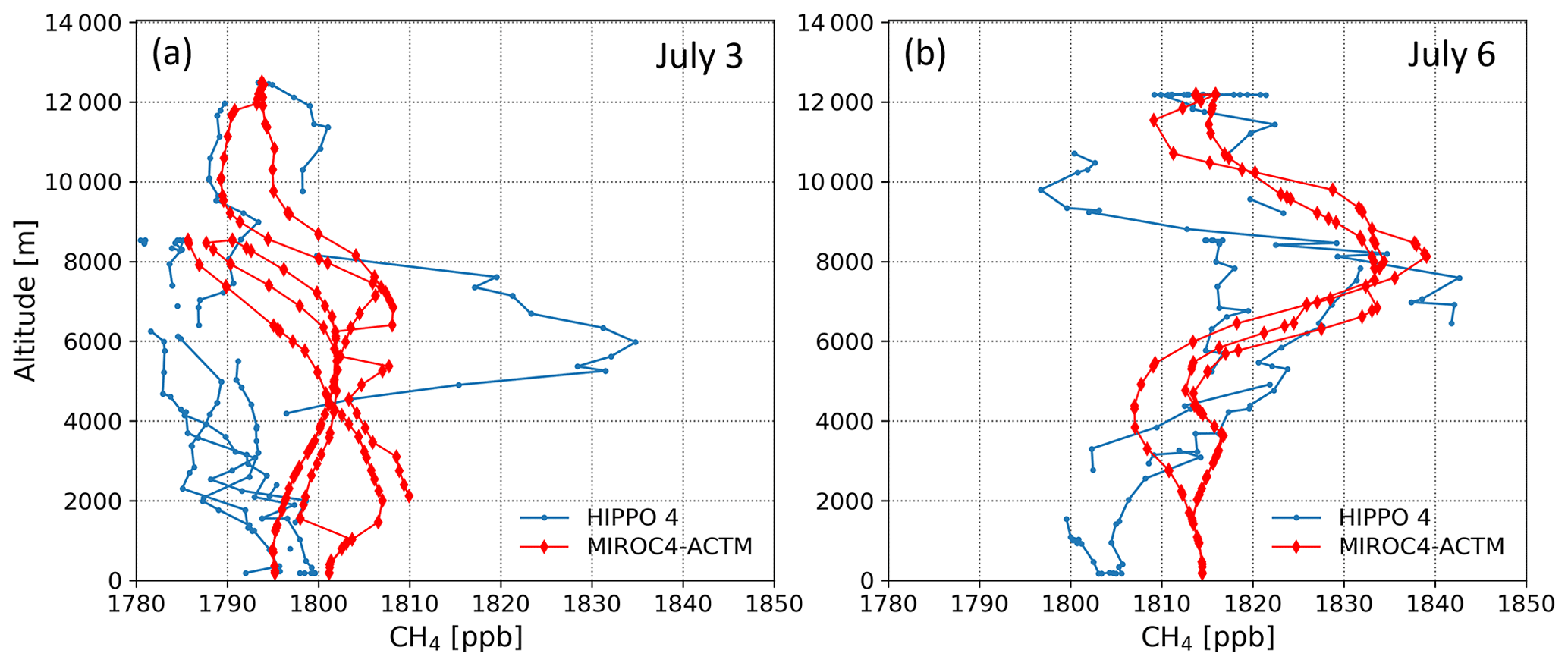
Figure A1 Comparison between HIPPO 4 (blue) and MIROC4-ACTM profiles (red) on 3 July (a) and 6 July (b) 2011.

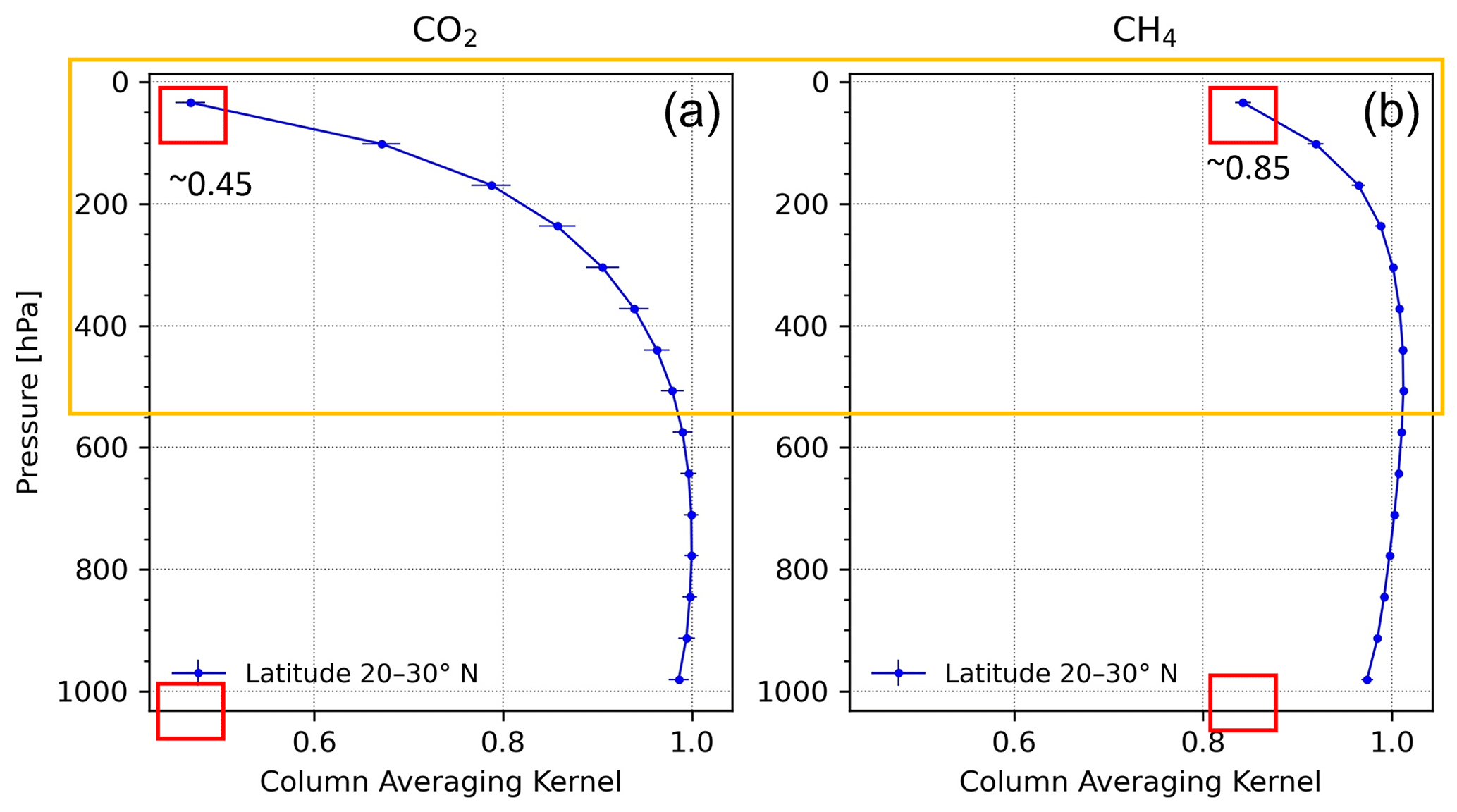
Figure A2 The GOSAT NIES column averaging kernel (ak) with the dependence on the pressure for CO₂ (a) and CH₄ (b) at the latitude range 20–30° N. The yellow square indicates the area of major differences; the red squares emphasize the difference in the ak value at the lowest pressure of 34 hPa. Compared to the ak of CO₂, the impact of the CH₄ profile on the calculated XCH₄ is high below the tropopause (400–200 hPa) and at the stratospheric part.

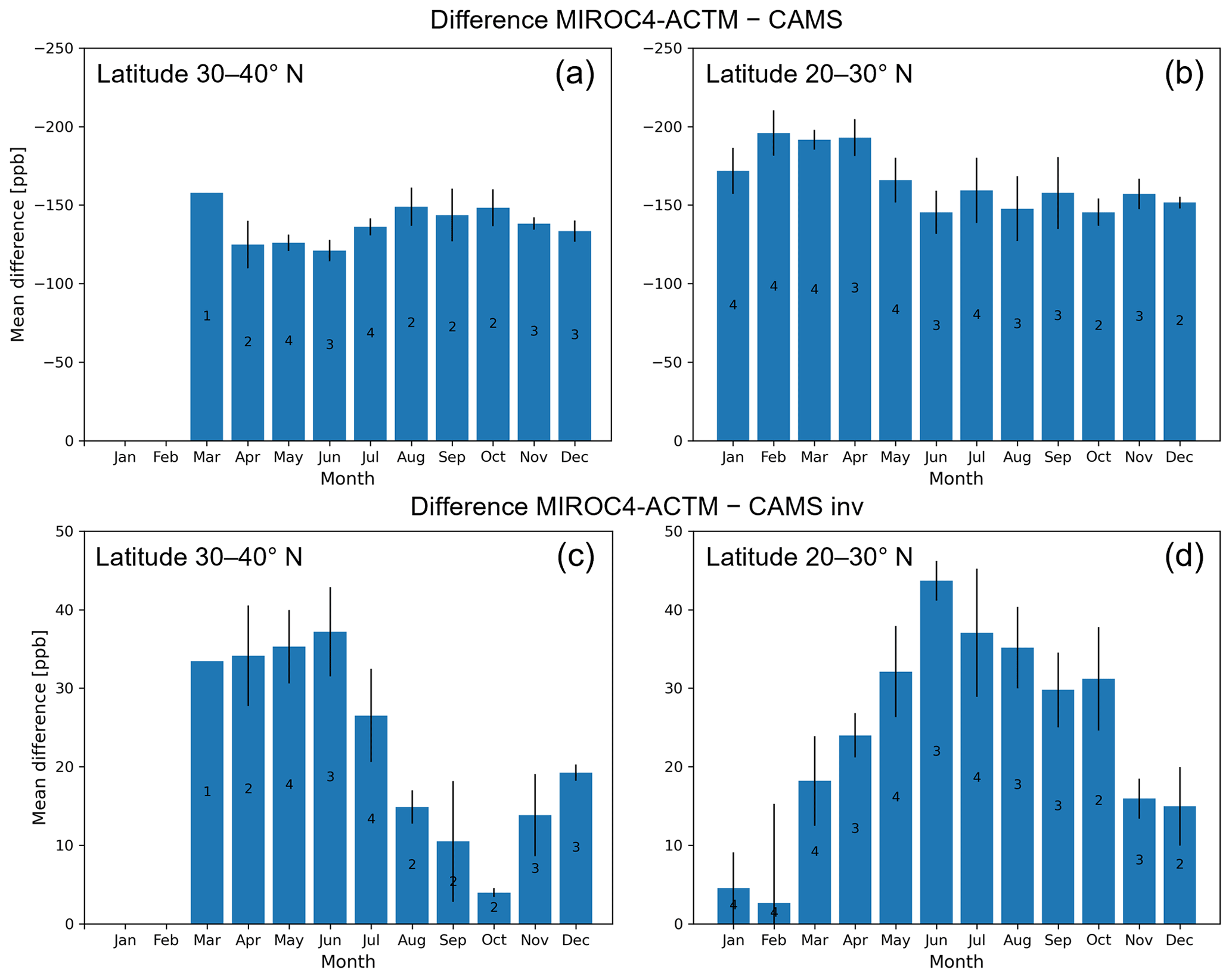
Figure A3 Monthly averaged difference between MIROC4-ACTM and CAMS (a, b) and MIROC4-ACTM and CAMSinv (c, d) at the latitude ranges 30–40 and 20–30° N, respectively. Error bars are the standard deviation of the monthly averages. Numbers inside the bars correspond to the number of mean values per month.

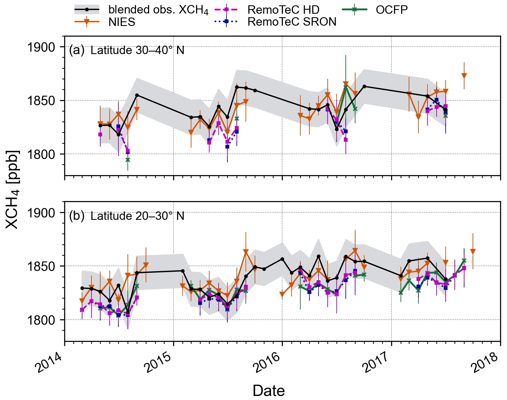
Figure A4 Temporal variation in the blended obs. XCH₄ (${\mathrm{ACTM}}_{{\mathrm{XCH}}_{\mathrm{4}}}$; black) in comparison with GOSAT XCH₄ retrievals from NIES (orange), RemoTeC Heidelberg (HD) (magenta), RemoTeC SRON (blue), and OCFP (green) at the latitude ranges, where g1 is 30–40° N (a), and g2 is 20–30° N (b). The gray area is the 16 ppb uncertainty range of the blended obs. XCH₄. The difference in RemoTeC HD – RemoTeC SRON is −0.4 ± 4.4 and 1.6 ± 3.0 ppb (mean difference ± standard deviation of differences) at g1 and g2, respectively. The average number of valid retrievals per month for RemoTeC HD (g1 is 20 ± 14 ppb, 13 months; g2 is 50 ± 29 ppb, 24 months) is larger than for RemoTeC SRON (g1 is 24 ± 16 ppb, 11 months; g2 is 41 ± 24 ppb, 24 months).