the Creative Commons Attribution 4.0 License.
the Creative Commons Attribution 4.0 License.
 | 29 Feb 2024
Level0 to Level1B processor for MethaneAIR
Eamon K. Conway
Amir H. Souri
Joshua Benmergui
Xiong Liu
Carly Staebell
Christopher Chan Miller
Jonathan Franklin
Jenna Samra
Jonas Wilzewski
Sebastien Roche
Bingkun Luo
Apisada Chulakadabba
Maryann Sargent
Jacob Hohl
Bruce Daube
Iouli Gordon
Kelly Chance
Steven Wofsy
This work presents the development of the MethaneAIR Level0–Level1B processor, which converts raw L0 data to calibrated and georeferenced L1B data. MethaneAIR is the airborne simulator for MethaneSAT, a new satellite under development by MethaneSAT LLC, a subsidiary of the Environmental Defense Fund (EDF). MethaneSAT's goals are to precisely map over 80 % of the production sources of methane from oil and gas fields across the globe to an accuracy of 2–4 ppb on a 2 km2 scale. Efficient algorithms have been developed to perform dark corrections, estimate the noise, radiometrically calibrate data, and correct stray light. A forward model integrated into the L0–L1B processor is demonstrated to retrieve wavelength shifts during flight accurately. It is also shown to characterize the instrument spectral response function (ISRF) changes occurring at each sampled spatial footprint. We demonstrate fast and accurate orthorectification of MethaneAIR data in a three-step process: (i) initial orthorectification of all observations using aircraft avionics, a simple camera model, and a medium-resolution digital elevation map; (ii) registration of oxygen (O2) channel grayscale images to reference Multispectral Instrument (MSI) band 11 imagery via Accelerated-KAZE (A-KAZE) feature extraction and linear transformation, with similar co-registration of methane (CH4) channel grayscale images to the registered O2 channel images; and finally (iii) optimization of the aircraft position and attitude to the registered imagery and calculation of viewing geometry. This co-registration technique accurately orthorectifies each channel to the referenced MSI imagery. However, in the pixel domain, radiance data for each channel are offset by almost 150–200 across-track pixels (rows) and need to be aligned for the full-physics or proxy retrievals where both channels are simultaneously used. We leveraged our orthorectification tool to identify tie points with similar geographic locations in both CH4 and O2 images in order to produce shift parameters in the across-track and along-track dimensions. These algorithms described in this article will be implemented into the MethaneSAT L0–L1B processor.
- Article
(5242 KB) - Full-text XML
- BibTeX
- EndNote


Methane (CH4) is a potent greenhouse gas that, despite having an atmospheric lifetime of approximately 12 years which is almost one-eighth that of carbon dioxide, has approximately 26 times the global warming potential (GWP) of CO2 over a 100-year time horizon. Over the first 20 years, methane has a GWP approximately 70–80 times that of CO2 (Forster et al., 2008). Analysis carried out by Etheridge et al. (1998) on ice-core samples extracted in the Antarctic peninsula showed that atmospheric methane concentrations have rapidly increased since the 1700s. These increases are predominantly anthropogenic, driven by industrialization and agricultural demand (Hmiel et al., 2020). In 2017, atmospheric levels of CH4 averaged 1850 ppb, triple the eighteenth-century limits of approximately 650 ppb (Nisbet et al., 2019). Despite knowledge of its large atmospheric warming potential, except for a “stabilization” period between 2000 and 2007, methane concentrations continue to increase (Turner et al., 2019). Preliminary results from the National Oceanic and Atmospheric Administration (NOAA) suggest that 2020 may have seen the largest increase in atmospheric methane concentrations since 1983 (NOAA, 2021).
Methane monitoring instruments such as the TROPOspheric Monitoring Instrument (TROPOMI) (Veefkind et al., 2012) can detect emission plumes to a 12 ppb precision on a 7 × 5 km2 scale (Pandey et al., 2019; Y. Zhang et al., 2020) at nadir. TROPOMI's 2600 km swath provides daily global coverage, which greatly increases our knowledge of emission hotspots on the Earth, but the coarse resolution makes it challenging to quantify and detect small-scale sources. MethaneSAT (MethaneSAT LLC, 2021) will be launched sometime in the first quarter of 2024, and the mission aims to precisely map over 80 % of the production sources of methane from oil and gas fields across the globe to an accuracy of 2–4 ppb on a 2 km2 scale, with a native spatial resolution of 400 m × 100 m (along- and across-track, respectively) at nadir, supporting the goal of reducing methane emissions from the oil and gas sector by 45 % by the end of 2025. It will have two spectrometers on board, an oxygen (O2) sensor and a methane (CH4) sensor, both of which will operate in the shortwave infrared region. Retrieving methane to this precision will require the instruments to be calibrated to a high level of accuracy. It is expected that a signal-to-noise ratio of approximately 1000 will enable this to be achieved. The CH4 sensor will observe between 1598 and 1683 nm, which encompasses the CO2 absorption features at approximately 1610 nm and the CH4 features at approximately 1650 nm. The O2 sensor will observe between 1249 and 1305 nm, encompassing the “singlet-delta” O2 band at approximately 1270 nm. The swath range will encompass approximately 200 km at an altitude of approximately 526 km, with ≈ 2000 pixels across the track, enabling the precise detection and identification of point source emissions.
It has been more common to use the oxygen A-band at 762 nm to determine the optical path length along the line of sight, with the SCanning Imaging Absorption spectroMeter for Atmospheric CHartographY (SCIAMACHY), Greenhouse Gases Observing Satellite (GOSAT), TROPOMI, and Orbiting Carbon Observatory-2 (OCO-2) all observing this band. Many experimental measurements of this band have hence been carried out to improve the quality of spectroscopic information (Drouin et al., 2017, 2013), which include the observation of electric quadrupole transitions (Miller and Wunch, 2012). However, recent efforts using cavity ring-down spectrometers have significantly improved the spectroscopic information of the singlet-delta band. Konefał et al. (2020) and Tran et al. (2020) have shown that prior transition intensities were incorrect by between 1 % and 3 %, a non-negligible and important improvement for the MethaneSAT mission. MethaneSAT will also need to model the airglow in this band, which can pose a challenge. However, despite this, recent advances in airglow simulations using SCIAMACHY data have used this band and excellent results are attainable (Sun et al., 2018; Bertaux et al., 2020), which shows that this band can be used for satellite remote sensing of greenhouse gases.
Airborne simulators provide an opportunity to develop and validate science algorithms prior to obtaining observation data from a forthcoming space-based instrument. Considering the NASA TEMPO (Tropospheric Emissions Monitoring of Pollution) (Zoogman et al., 2017) geostationary satellite mission that will operate in the visible and ultraviolet spectral regions, Geostationary Trace gas and Aerosol Sensor Optimization (Geo-TASO) (Leitch et al., 2014; Nowlan et al., 2016), the Airborne Compact Atmospheric Mapper (ACAM) (Kowalewski and Janz, 2009; Lamsal et al., 2017; Nowlan et al., 2018), and the GEOstationary Coastal and Air Pollution Events (GEO-CAPE) Airborne Simulator (GCAS) are examples of airborne simulators that have provided the resources to design and enhance the retrieval algorithms. In the SWIR, AVIRIS (Thompson et al., 2016), MAMAP (Gerilowski et al., 2011), GHOST (Humpage et al., 2018), and JAXA's airborne instrument (Kuze et al., 2020) have been utilized to retrieve methane emissions. The airborne simulator for MethaneSAT is appropriately named MethaneAIR, and it includes two spectrometers scanning almost the same SWIR regions as MethaneSAT. A total of 10 research flights have been completed in different parts of the US, with the final flight consisting of airglow observations. These research flights provided high-quality observation data to develop a fully automated MethaneAIR L0–L1B processor. The datasets have proved invaluable in developing science algorithms for MethaneSAT. Four additional research flights were performed in the fall of 2022 but will not be considered in this paper.
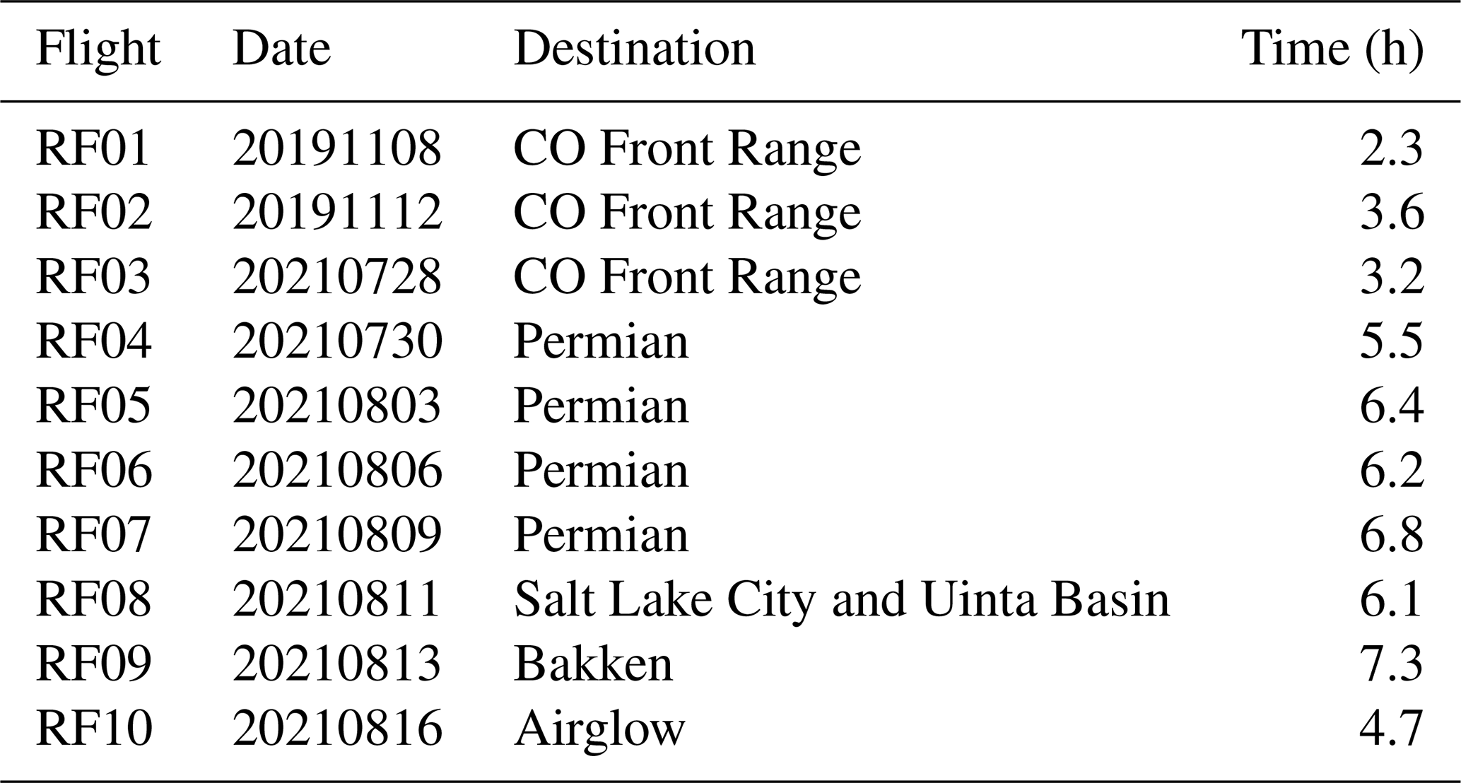
Table 1Shown below are the details for each MethaneAIR deployment, including destination and approximate length of observation
It is not uncommon for instrument properties such as wavelength registration and instrument line shape to slowly deviate away from the measurements recorded on the ground (Sun et al., 2017a, b; Voors et al., 2006; Cai et al., 2022). Such variations can be a result of the vibration during the initial launch of the instrument or from the differences between the environmental conditions encountered in the air (or space) versus the laboratory setup on the ground. It is therefore quite useful to routinely perform in-flight calibration measurements to monitor any possible changes. For OCO-2, Sun et al. (2017b) analyzed the observed instrument line shape (ILS) and wavelength registration and compared these to the ground-based calibration measurements. Several line shape models were tested: super-Gaussian (Beirle et al., 2017), Gaussian, stretch and squeeze of the pre-flight ILS, and a hybrid mix of Gaussian functions (Liu et al., 2015). It was found that the flat-top nature of the OCO-2 ILS made the Gaussian function unsuitable; however, reasonable results were obtained with the other models. While TROPOMI has dedicated onboard calibration light sources (van Hees et al., 2018; Van Kempen et al., 2019), the laboratory-measured wavelength calibration parameters (Kleipool et al., 2018) are not optimized in the L0–L1B processing, but rather during trace gas retrievals in the L1–L2 processing.
The MethaneAIR spectral calibration measurements have already been described in great detail by Staebell et al. (2021): wavelength, radiometric properties, and stray-light properties, together with the instrument response function (ISRF), were derived for each of the CH4 and O2 spectrometers. The measured data have been implemented into the MethaneAIR L0–L1B processor. In this article, the development of the L0–L1B processor will be described in detail.
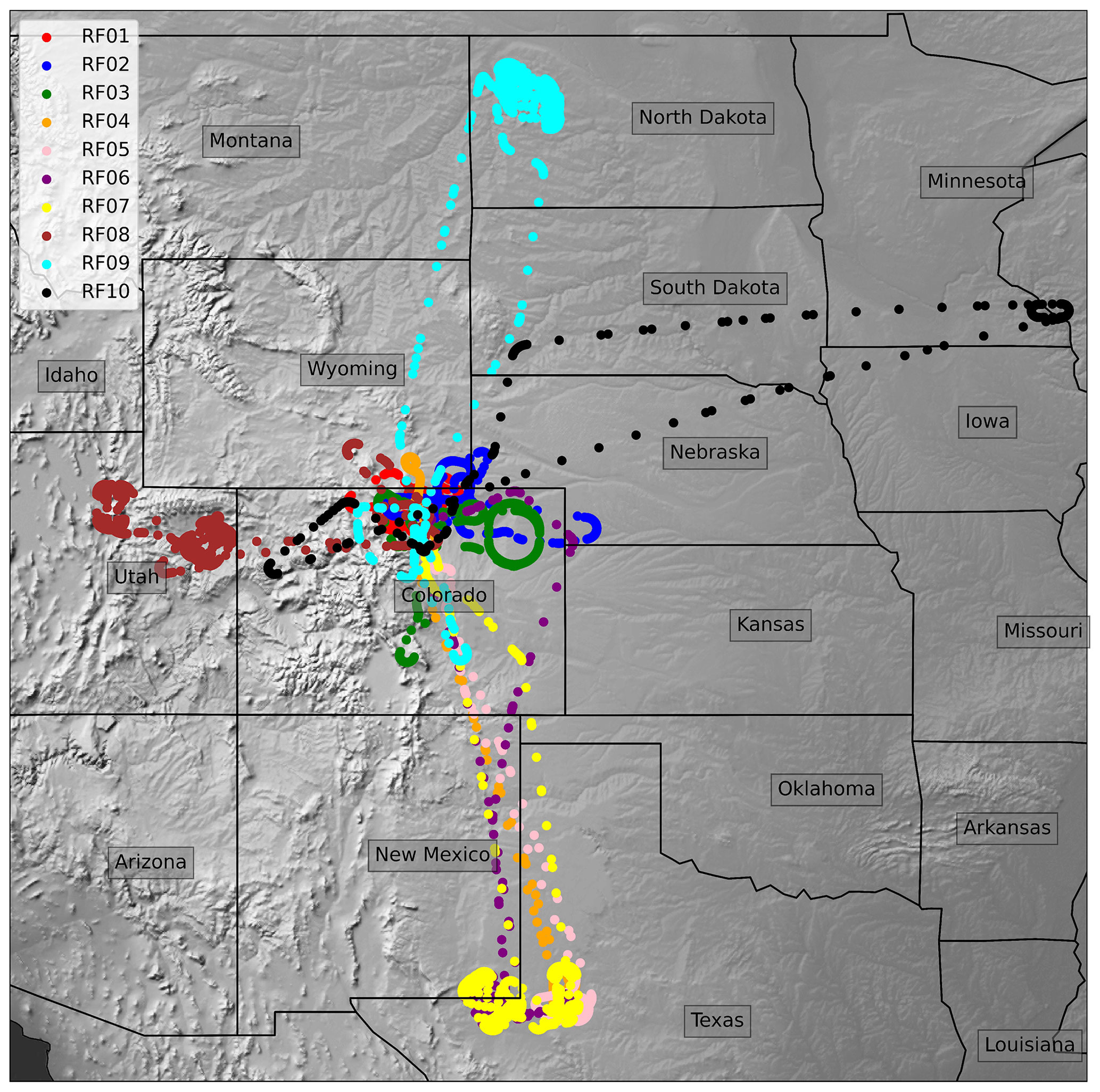
Figure 1Map of the MethaneAIR research flights.
2.1 The MethaneAIR instrument
The MethaneAIR instrument closely echoes the design of MethaneSAT. Two spectrometers, one measuring methane spectra and the other oxygen spectra, were integrated side by side onto the National Science Foundation (NSF) Gulfstream V (GV) aircraft that is controlled by the National Center for Atmospheric Research (NCAR) (NCAR – Earth Observing Laboratory, 2005). Each of these detectors possesses 1024 spectral pixels (columns) and 1280 spatial pixels (rows). The bandpass for the CH4 sensor covers 1592–1680 nm, while the O2 sensor spans 1236–1319 nm. Of the 1280 rows, only indices 135–997 and 308–1170 are illuminated in each of the respective CH4 and O2 sensors. The native spatial resolution of MethaneAIR observations is approximately 25 m (along-track) × 5 m (across-track) for a typical flight altitude of 9 km. More details of the MethaneAIR instrument are described by Staebell et al. (2021).
2.2 Research flight details
The dates, destinations, and observation times of the 10 research flights we will consider in this paper are described in Table 1 and Fig. 1. In total, approximately 50 h of observation data were recorded for MethaneAIR. The first two flights, RF01 and RF02, which occurred in late 2019, were engineering flights, whose purpose was to ensure that the instrument was operating as expected. Over these two flights, 5.8 h of observation data were collected in the Colorado Front Range. More flights were planned to occur at this time; however, flights ended due to GV maintenance issues and were rescheduled for a later date. Due to the COVID-19 outbreak, these rescheduled MethaneAIR flights were further delayed until the summer of 2021. Hence, these engineering flights proved to be critical contributors to the development of the science algorithms of both MethaneAIR and MethaneSAT.
RF03 was the first of these new flights and it covered a similar region as RF02. Its purpose was to validate both the instrument performance and science algorithms via comparisons to RF02, prior to mapping out targets encompassing oil and gas infrastructure. For RF04–RF07, MethaneAIR mapped out regions of the Permian Basin over the course of 25 h (including transit time from Colorado). During RF04 and RF05 research flights, numerous passes over controlled methane release experiments also occurred. These releases provide valuable ground truth to evaluate our methane retrieval and emission estimate algorithms.
Almost 6.1 h of observation data were collected during RF08, which targeted Salt Lake City and the Uinta Basin. For RF09, the Bakken oil and gas region that encompasses North Dakota was the designated target. For visual context, a map detailing the flight paths of RF01–RF09 is shown in Fig. 1. RF10 was dedicated to investigating airglow emission, a key challenge for MethaneSAT's observations in the O2 singlet-delta band. To measure airglow emission, the MethaneAIR payload was rotated 180° so that the O2 sensor could look vertically out of the upper port aboard the NCAR/GV aircraft.
Figure 2 displays the processes of the L0–1B algorithm. Each processing step is described below from Sect. 3.1 through Sect. 3.8, and the process is fully automated. For 30 s of L0 data, which is the amount of time assigned to each individual observation granule (L0 file), the CPU time is approximately 90 min. Most of the run time is dedicated to the orthorectification procedures, primarily the final optimization procedure. The orthorectification procedure shown in Fig. 2 is within a dashed enclosure as the process has two separate steps to it. The final one is a refinement procedure and is technically optional but provides more accurate geospatial information on the pixels. The L0–L1B processes have also been configured to operate in a cloud environment, and for future flights of MethaneAIR, processing will be done in the cloud.
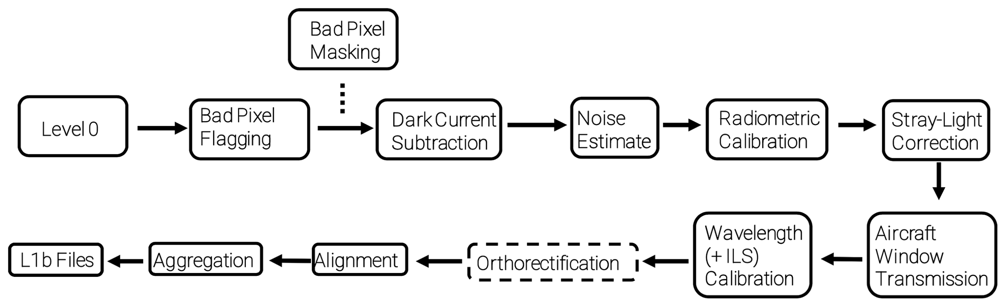
Figure 2Flowchart representation of the processes within the MethaneAIR L0–L1B processor. The orthorectification process is in a dashed box to show that it is written in R code and imported into Python.
3.1 Dark current and bad pixel flagging
During each of the research flights, dark collects were obtained at different instances during the flights and each was used to filter bad pixels according to their standard deviation from the mean. By averaging together all frames in each of the 30 s collects in the along-across direction, a mean dark current was derived and a 3σ limit was used to identify the bad pixels, i.e., pixels whose signals deviate from the mean by more than 3σ. Applying this limit to each sensor, an average of 1617 and 467 bad pixels were identified in each of the O2 and CH4 sensors, respectively. Staebell et al. (2021) used a similar approach to flag bad pixels using a 3σ deviation limit from the linear fit of the gain of each sensor.
These bad pixels were flagged and/or masked in all subsequent processes. Next, the mean dark current is subtracted from each illuminated collect to yield dark-corrected frames.
3.2 Noise estimate
The XCH4 retrieval follows an optimal estimation framework adjusting the concentration of several absorbing trace gases and atmospheric states (i.e., temperature and pressure) to best match the observed radiance. The noise model determines the uncertainty of the observed radiance populating the covariance matrix of observations in the retrieval algorithm. Good knowledge of the noise level is critical in reducing the contributions of observational errors to the retrieved XCH4. Using the dark collects, read noise (Nr) is calculated for each pixel by considering the standard deviation of the signal across the number of frames collected. Combining the mean dark current (D) in units of digital number (DN), measured raw signal (S) in DN, gain (g) in units of electrons per DN, and the number of dark frames (Nf) with the electronic offset (ϵ) in DN, the noise (in DN) of a particular pixel is calculated via Eq. (1). The electronic offset was determined to be 1500 DN during the laboratory calibration and is the dark signal expected for an integration time of zero. The CCD gain, defined as the slope of the variance to the median signal, was determined to be 4.6. These values will be converted to radiance and stored in the L1B files.
3.3 Radiometric calibration
Radiometric calibration converts raw sensor data in units of DN to radiance units. The radiometric calibration is based on laboratory measurements using an integrating sphere with a calibrated broadband light source. A fifth-order polynomial is derived and subsequently applied to each illuminated pixel, whose coefficients originate (for RF01 and RF02) from the radiometric calibration measurements to convert DN to photons s−1 cm−2 nm−1 sr−1. After the first two research flights were concluded, newer radiometric calibration files were created after an extensive calibration effort using the same approach as Staebell et al. (2021). These newer coefficients were utilized in the processing of RF03–RF10. In situations in which we have only a small number of dark current collects for a research flight (fewer than two for RF01 and RF02), it can increase the possibility of random telegraph signals (RTSs) going unchecked if a second bad pixel filtering procedure is not implemented on the illuminated scenes. Hence, to screen for extreme outliers, any pixel with radiance over 1015 photons s−1 cm−2 nm−1 sr−1 or below 1010 photons s−1 cm−2 nm−1 sr−1 is also flagged as a bad pixel during processing. These limits were chosen as they are outside the expected operating range of the sensors. In addition to the bad pixel map, two pixels were found to be problematic in the CH4 channel of the first two research flights and were hence flagged. The radiometric calibration coefficients were identified to be the source of this error and were masked. None were captured in RF03–RF10, which used new calibration measurements.
3.4 Window transmission
The GV was equipped with an anti-reflection coated window and for the wavelengths we are interested in of 1236–1680 nm, the aircraft window transmittance changes smoothly from 99.7 % to 98.1 %. To account for the window transmittance, we divided the raw signal in DN by the transmittance.
3.5 Stray-light correction
Stray light is undesirable electromagnetic radiation that reaches the sensor and interferes with performance, and it can occur for various reasons, such as when light reflects off the mechanical surfaces internal to the optical system, leakage of light through a gap in the system, or from light scattering off dust in the system. The MethaneAIR sensors were designed to minimize the presence of stray light. Ground calibration efforts confirmed that less than 2 % of the total light recorded by the sensors is traceable to stray-light effects. A full description of the characterization of MethaneAIR stray-light kernels is described by Staebell et al. (2021), but we briefly describe it here. The stray-light correction algorithm of Staebell et al. (2021) is based on the method used to correct the stray light in TROPOMI (Tol et al., 2018). The central region of 15 spectral × 11 spatial pixels of the stray-light kernel is defined as in the band, and the kernel values in the central region are set to zero so that the stray-light correction is applied to pixels outside this central area. This modified kernel is referred to as the far-field kernel and was utilized in the stray-light correction algorithm, where the light is iteratively deconvolved and redistributed.
3.6 Wavelength and ILS calibration
Successful trace gas retrievals rely on accurate knowledge of the observed wavelength and the instrument line shape (ILS). Laboratory calibration efforts were carried out to measure these values pre-flight (Staebell et al., 2021); however, it is relatively common for the observed wavelength to deviate from the laboratory-calibrated measurements during operation. It is, therefore, necessary to supplement this process with a wavelength-fitting routine to adjust the coefficients during flight. Also, unlike TROPOMI, the MethaneAIR and MethaneSAT instrument configurations are not designed to allow us to accurately monitor the instrument line shape (ILS) during operation with calibrated onboard lasers. We therefore added a forward model into the L0–L1 processor that can reliably detect abrupt changes in the ILS during flight; however, this process is optional in the L0–L1B processor for MethaneAIR because precise inverse modeling occurs during the L1–L2 processing step where wavelength and ILS fitting parameters are retrieved. The forward model we consider begins with a high-resolution (HR) (0.001 nm) solar spectrum (Coddington et al., 2021), where λ is the wavelength. The parameterization of λ with respect to the spectral pixel index is assumed throughout.
The first term in our forward model above, A, is the Lambert–Beer term that accounts for light attenuation in the atmosphere due to the presence of gases, which we will consider to be made up of water, methane, and oxygen. The next, B, is a high-resolution solar spectrum. C describes the slit function or ILS, which is derived from parameters pi. D is a polynomial scaling term, and finally E is a baseline correction term. The integration variable (λ′) spans the wavelength range of the convolution. δλ represents the wavelength shift. Alk represents variables that are optimized in the fit and scale the absorption factors (A, B, and C). Bj also represent numerical values that are optimized and shift the observation.
For CH4, cross sections are calculated from the line-by-line parameters in the HITRAN2020 (Gordon et al., 2021) database using the Voigt profile on a 0.001 nm grid for a variety of temperatures and pressures that cover the standard US atmosphere ranges. For O2–O2 collision-induced absorption (CIA), we attempted to use several sources of data in our model, each of which is theoretically, experimentally, or empirically derived. For theoretical CIA, we attempted to utilize the calculations from Karman et al. (2018), which we obtained from HITRANonline (Karman et al., 2019); for the experimental source, we tried to use the measurements from Maté et al. (1999), while we also considered the empirical TCCON CIA. For the absorbing species, the cross sections are weighted according to the standard US atmosphere with temperature (T) and pressure (P) at atmospheric layer i:
where SCDgeo refers to the geometric slant column density.
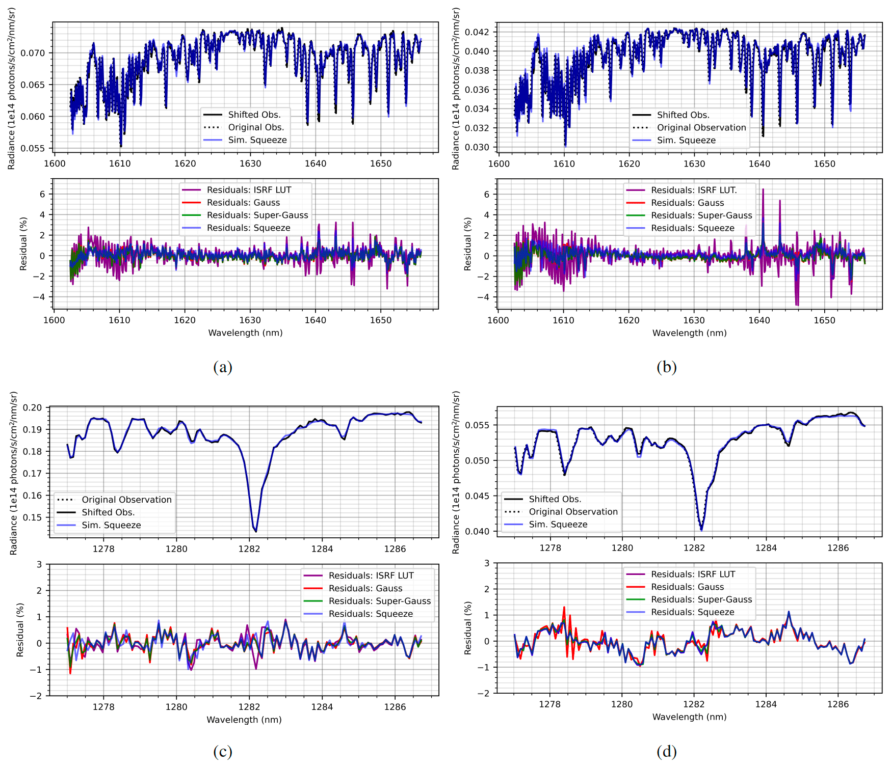
Figure 3Example spectrum fits to RF01 and RF02 for CH4 (a, b) and O2 (c, d) channels, respectively, using various ISRF models: laboratory-measured values as well as Gaussian, super-Gaussian, and squeeze of ISRF LUT. Only the squeeze model simulation spectra are shown in the upper panels to enhance the visibility of the observed wavelength shift.
The high-resolution data need to be convolved with respect to the measured ILS, which was probed at a number of wavelengths for both channels. For the methane channel, we have nine ISRF measurements at 1593, 1600, 1610, 1620, 1630, 1640, 1650, 1660, and 1670 nm, while for the oxygen channel we have 10 measurements at 1254, 1261, 1268, 1275, 1282, 1289, 1296, 1303, 1310, and 1317 nm. The ILS at the unmeasured wavelengths was determined by interpolating the measured data points. The forward model has the option of fitting each ISRF using either a squeeze or stretch parameter applied to the LUT values or a normalized Gaussian or super-Gaussian function. The parameters describing the slit function L are denoted as pi(λ) where the index runs over the number of possible parameters needed in each function for each ISRF: the Gaussian model has only one, and a squeeze or stretch has one, while the super-Gaussian possesses have two variables.
In Fig. 3, the results of a single fit to observed O2 and CH4 spectra taken during RF01 (a, c) and RF02 (b, d) are demonstrated. In each case, 100 along-track frames have been aggregated together to enhance the signal-to-noise ratio. In all cases, a third-order polynomial was used to fit a baseline, while a constant shift parameter was found to provide the best results. The retrieval wavelength range will not be the same as the wavelength range considered for the derivation of the wavelength calibration in this process. This fitting procedure is to derive the wavelength shift that occurs during flight, not to retrieve CH4. The quantum efficiency of the instrument decreases towards the ends of the spectra and can increase the noise in the fit; hence the ends were omitted.
In Fig. 3a and b, example fits in the CH4 channel are presented for the engineering flights, RF01 and RF02. In both instances, modeling the ILS with a Gaussian, super-Gaussian, or squeeze–stretch term is shown to provide lower residuals when compared to a simulated spectrum using the initial look-up table of ISRFs, derived by Staebell et al. (2021). It is apparent that there are significantly lower residuals in RF01 than in RF02, and this can be explained by the cabin temperature not being controlled during RF02 and the fact that the signal is higher in RF01. Analyzing both of these figures, it is quite clear that the measured ISRF FWHMs are too narrow. For the CH4 band at 1630–1650 nm, the forward model can simulate the dominant observations with an average residual of 1 %–2 % with either a Gaussian, super-Gaussian, or squeeze model, while using the LUT ISRFs yields residuals closer to 3 %–6 % in the strong absorption features. At shorter wavelengths near 1605 nm, the residuals for the CO2 band are within 1 % with each of a Gaussian, super-Gaussian, or squeeze ISRF model.
For RF02, the wavelength was observed to shift between 0.12 and 0.15 nm throughout the flight, a large portion of which is likely due to the temperature variation on board. The shift is also cross-track-dependent. For RF03, the wavelength shift was significantly larger, averaging 0.2 nm. The wavelength shifts for the remaining flights were significantly lower, averaging approximately 0.01–0.05 nm. The derived wavelength shifts in all cases were rather insensitive to the choice of slit function used in the forward model.
For the oxygen singlet-delta band, simulating the strong Q branch was shown to be very problematic. Regardless of our choice of reference CIA data or baseline polynomial, reasonable fitting results were not achievable using data from either research flight. We believe the difficulty is due to a combination of the CIA not being modeled correctly, large variations in the ISRF, and the simplicity of the forward model. Hence, we instead consider fitting the solar line at approximately 1282 nm and remove CIA as an absorbing species in the forward model. For each ISRF model considered, including the ISRF LUT values, residuals averaging less than 1 % are attainable. This is true for all research flights. Example fits are shown for RF01 in Fig. 3c and RF02 in Fig. 3d. For all flights, wavelength shifts in this channel are reasonably smaller than their CH4 counterparts, averaging less than 0.05 nm.
The observed ISRF FWHMs for all research flights deviate from the laboratory-measured values from Staebell et al. (2021). As an example, we consider RF02, which was a flight where the variation is considerably large, evident from Fig. 3a and b. Lower residuals are attainable for observations recorded in other research flights, likely a consequence of cabin temperature being controlled and monitored during flight; however, for RF02, the temperature was much less stable (not recorded). While this is clearly not an ideal situation for performing science retrievals, it does present the perfect opportunity to develop robust science algorithms.
The temperature variation in the aircraft cabin likely resulted in the ILS changing throughout the RF02 flight. In Fig. 4, the LUT ISRF data are fitted with a Gaussian line shape and the resulting FWHMs are compared to the retrieved Gaussian FWHMs deduced from RF02 data at wavelengths 1610, 1620, 1630, 1640, and 1650 nm. The results shown are for a 30 s granule captured when the aircraft was at 2.26 km and the granule consists of over 100 frames which were aggregated along-track. Dramatic changes in each ISRF are evident and differences of up to approximately 30 % are observed in the FWHM. The pattern seems to be almost reversed with respect to the across-track dimension, evidence of large environmental changes surrounding the instruments on board. Despite these large variations, relatively low residuals are obtained during wavelength calibration.
3.7 Orthorectification
Orthorectification is the process of mapping camera projections onto the Earth's surface to accurately determine the geolocation of the measurements. In order to pinpoint the exact location of methane emission sources, retrievals of column-average mole fractions of methane (XCH4) from MethaneAIR data have three major sensitivities to orthorectification accuracy.
-
The MethaneAIR instrument is composed of separate cameras for O2 and CH4 bands that must be spatially registered and aligned.
-
The retrieval algorithms require information about surface properties that vary widely over small spatial scales.
-
The retrieval algorithms require information about the viewing geometry of the measurements.
The aim is to orthorectify the imagery to an accuracy of approximately 30 m, which is sufficient to pinpoint the emission source. Note that the sensitivity of the retrieval algorithms to the viewing geometry is not only a sensitivity to the camera projections onto the Earth's surface but also a sensitivity to the position and attitude of the camera itself. We apply an orthorectification procedure that makes a first guess using the aircraft avionics, then refines the mapping to the Earth's surface with an image registration algorithm, and finally refines the position and attitude of the cameras with a bundle adjustment algorithm.
Orthorectification requires a model of the camera position and attitude (the extrinsic model), a model of the camera pixel projections (the intrinsic model), and a model of the Earth's surface (a digital elevation model or DEM).
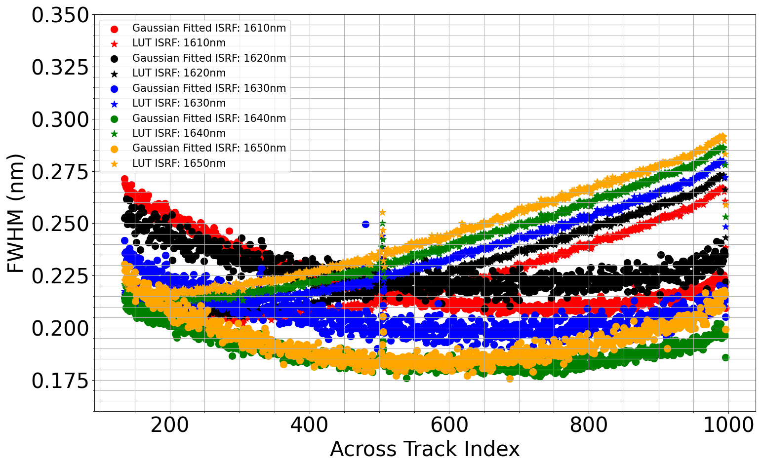
Figure 4Retrieved ISRF FWHM using a Gaussian model obtained from a 30 s granule in RF02 compared to the laboratory ISRF that was fit to a Gaussian for equal comparison.
Our first guess of the orthorectification uses an extrinsic model based on the aircraft's onboard avionics system. The onboard avionics system consists of two identical Honeywell LASEREF III/IV inertial reference units (IRUs) and a Garmin Model OEM WASS GPS-16 unit (GPS) (NSF/NCAR Gulfstream V Investigator's Handbook, https://www.nasa.gov/pdf/594185main_gv_completehandbook.pdf, last access: 15 April 2023). We use the position from the GPS-corrected IRU longitude and latitude, GPS altitude (altitude above mean sea level plus the geoid height), and IRU true heading, pitch, and roll. These systems have a stated accuracy of ±15 m in horizontal position, ± 10 m in vertical position, ±0.05° pitch and roll, ±0.2° in true heading. Sharp changes in attitude can affect the accuracy of the GPS unit and cause discontinuities in the aircraft position measurements. This was observed during the MethaneAIR flights. Additional attitude errors can result from the alignment and damping of the instrument mounting. As a result, our first-guess orthorectification extrinsic model has substantially larger uncertainty than that reported in the avionics.
We apply a simple intrinsic model using a fixed-focal-length camera model with no distortion, distributing pixels at equal angles about the boresight (, where f is the focal length and θ is the field of view of 33.7°). MethaneAIR used an Edmund Optics 16 mm focal length lens for 1′′ sensor format (https://www.edmundoptics.com/p/16mm-focal-length-lens-1quot-sensor-format/17861/, last access: 15 April 2023). The lens has a reported TV distortion of < 1 %.
DEM maps were created during processing using the United States Geological Survey (USGS) 3D Elevation Program (3DEP) 1 arcsec data, gathered via the Python py3dep package. To cover regions beyond the US for future flights we will replace this dataset with the global ALOS DEM at 30 m resolution using our Python demalos package (https://github.com/ahsouri/demalos, last access: 15 April 2023).
Orthorectification of remotely sensed imagery is a complex process, and many of the methods and approaches are described in depth by Baiocchi et al. (2020). The orthorectification algorithm for MethaneAIR proceeds as follows.
-
Calculate the aircraft position in meters in an Earth-centered, Earth-fixed (ECEF) coordinate system from the longitude, latitude, and elevation, assuming geodetic coordinates on the WGS84 ellipsoid.
-
Calculate unit vectors for the tangent frame to the WGS84 ellipsoid (north–east–down) at the aircraft position.
-
Calculate unit vectors of the aircraft frame by applying intrinsic rotations to the tangent frame about the true heading, pitch, and roll.
-
Calculate the camera boresight (assumed to be +z in the aircraft frame).
-
Calculate individual pixel boresights by applying an additional rotation about the aircraft x axis according to the intrinsic model.
-
Calculate reference vectors from each point on the DEM to the aircraft.
-
Snap the pixel boresights to the reference vectors (i.e., find the closest reference vector using Euclidean distance in R3) to find the surface elevation for each pixel projection.
-
Calculate the intersection of the pixel projection with an ellipsoid equal to the WGS84 ellipsoid adjusted to the surface elevation.
-
Calculate the geodetic longitude and latitude of the intersection of the pixel projections with the Earth.
This algorithm's trade-off between speed and accuracy depends on the resolution of the DEM. When computing the orthorectification for output, we use the DEM with the full 1 arcsec. When optimizing the aircraft position and attitude during bundle adjustment, we aggregate the DEM to 8 arcsec (applied to the reprojection and the registered image).
We estimate the sun position using the Astronomical Almanac 2020 algorithm and transform from Earth-centered inertial (ECI) coordinates to ECEF by propagating through precession, nutation, Greenwich hour angle, and polar motion matrices using Earth orientation parameters from the International Earth Rotation and Reference Systems Service (IERS) Bulletin.
A fully automatic geometric correction, which refers to removing geometric distortions in raw images with respect to an orthogonal view of a reference image, is developed using a computer vision image registration method. We apply image registration to the avionics-based MethaneAIR imagery procedure in a two-step process: geographically matching (i) the MethaneAIR O2 imagery to cloud-free orthorectified Multispectral Instrument (MSI) (Sentinel-2) band 11 reflectance (1610 nm) at the top of the atmosphere and (ii) CH4 imagery to the rectified MethaneAIR O2 imagery. We call the first (second) step the absolute (relative) correction. In the first step, the use of the MethaneAIR O2 channel is preferred over the CH4 channel due to the presence of stronger signal-to-noise ratios. The clear-sky MSI imagery (<3 % cloud in each scene covering 100×100 km2) at the resolution of 20 m is taken at the nearest time with respect to that of the MethaneAIR acquisition, enabling us to minimize the potential differences in the surface features changing over time. We reduce the atmospheric interference by averaging the MethaneAIR radiance within the atmospheric windows of 1250–1255 and 1620–1630 nm for O2 and CH4, respectively. To be able to automatically extract distinctive points (called key points) from the images, we leverage a multi-scale feature extraction method called accelerated KAZE (A-KAZE) (Alcantarilla et al., 2013). This method uses a scale-based nonlinear diffusion filter to describe distinctive features (i.e., corners, lines, patterns, etc.) while reducing noise and simultaneously retaining the boundaries of objects. An adaptive histogram equalizer with a window of 8×8 is used to enhance the image contrast, which is found to be advantageous in increasing the number of key points. Subsequently, A-KAZE determines extrema by comparing filtered images by the diffusion filter at different scales (i.e., less to more blurred) in a window of 3×3 pixels. Low-contrast key points are eliminated by fitting a 2D quadratic function. Each key point is then described by a 3-bit descriptor encapsulating radiance intensity as well as vertical and horizontal gradients pertaining to patches neighboring the key point based on the modified local difference binary (M-LDB) method described in Alcantarilla et al. (2013). It is worth noting that each patch is defined based on the gradient vector, which in turn makes the algorithm invariant to scale and rotation. We score the Hamming distance between key points generated from both MSI and MethaneAIR to determine which features in each image map to each other. We use the Hamming distance to remove the irrelevant features based on a fixed threshold and use a brute-force matcher to pair them. A robust outlier detector called random sample consensus (RANSAC) is applied to the paired key-point candidates with more than 10 000 iterations and a residual error threshold of 0.0005°. The RANSAC algorithm is discussed in great detail by H. Zhang et al. (2020). This algorithm ultimately provides a linear relationship between the geographic latitudes and longitudes of the paired key points extracted from the target (unrectified) image with respect to those from the reference one. This linear relationship mathematically explains varying scales and translations between two images, allowing for rectifying major geometric misalignment. This algorithm is called GeoAKAZE, which is publicly available in Souri (2022).
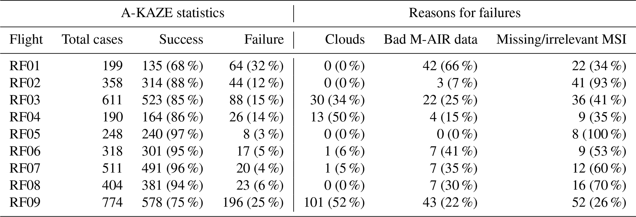
In terms of the absolute correction, we run the geolocation algorithm on the entire set of MethaneAIR flights without sub-optimally modifying the parameters defined in the algorithm, including the number of RANSAC iterations and the size of the histogram equalizer window. The approach was found to be successful, with the results displayed in Table 2. These numbers are estimated based on assessing individual paired images and considering the residuals obtained from the linear fit. The success and failure metric is determined by analyzing the correlation between the matched points that are obtained from the RANSAC algorithm. If the slope deviates more than 10 % from unity or the Pearson correlation coefficient deviates more than 5 % from unity, the match is considered a failure. The relatively poor performance in the RF01 data likely arises from a combination of the aircraft's low altitude and/or passes over mountainous terrain. Figure 5a depicts some instances of excellent proficiency of the method in orthorectifying the MethaneAIR O2 images to MSI, while Fig. 5b shows examples of the respective mapping of CH4 to O2. The background picture for (a) is taken from the MSI band 11 (the reference image), and the overlaid picture is from MethaneAIR O2, while for (b), the background is O2. It is readily evident that features such as roads, farms, and buildings are better lined up after the corrections.
The spatial error associated with the avionics-only orthorectification data is depicted in a whisker plot image; see Fig. 6. RF01 has the largest range of errors of any flight, perhaps due to variable flight height and maneuver (Table 2). Except for this flight, the mean value of the median spatial error across the flights is approximately 600 m, which is over an order of magnitude greater than the native pixel resolution. This necessitated implementing the GeoAKAZE procedure to all flight data.
Table 2Statistics from the orthorectification GeoAKAZE procedure for the MethaneAIR (M-AIR) research flights.
As for the relative correction, the success rates are found to consistently be over 95 % for all the research flights of MethaneaAIR (not shown in Table 2). Since MethaneAIR O2 and CH4 radiances are captured at (nearly) the same time, geometry, and environment, we observe higher success rates compared to the absolute correction, indicating a strong degree of relevancy between the radiances.
Following this, we attempt to optimize the aircraft avionics (position and attitude of the aircraft) to the GeoAKAZE-corrected pixel projections to produce optimized viewing geometry. The optimized avionics result in values of the viewing zenith angle, scattering angle, and geometric air mass factor consistent with the observed imagery. We use the limited-memory Broyden–Fletcher–Goldfarb–Shanno algorithm over a bounded domain (Byrd et al., 1995) to derive the corrections to the aircraft position (m ECEF) and attitude (degrees pitch, roll, true heading) that produce the minimum difference between the pixel projections and the GeoAKAZE-corrected pixel projections. In cases in which the optimized correction falls near the edge of the domain (initialized to 200 m or 10° in each direction), we note the case for quality control checks, expand the domain, and recompute the optimization. We compute the optimization independently for each data granule. This may result in small discontinuities in the orthorectification within the tolerance of the orthorectification error.
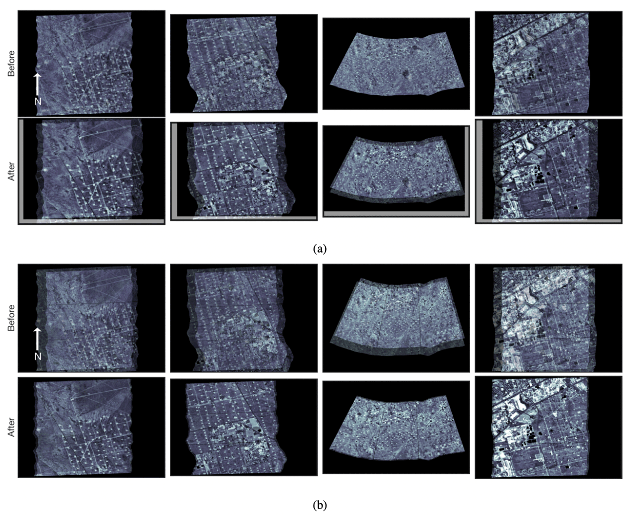
Figure 5Shown in (a) is MSI band 11 imagery (background) overlaid by the spectrally averaged MethaneAIR O2 channel (foreground) before applying the geolocation correction (first row) and after (second row). In (b), the spectrally averaged MethaneAIR CH4 channel (foreground) overlays spectrally averaged MethaneAIR O2 channel data (background) before applying the geolocation correction (first row) and after (second row). Note that surface features are markedly aligned between images after the adjustment.
When the GeoAKAZE process fails, the orthorectification optimization procedure cannot occur. Therefore, the L1B data utilize the less accurate avionics-only orthorectification data, which are always available. On the contrary, where the GeoAKAZE is successful, it is still possible for the optimization procedure to fail, either due to the optimizer failing to converge or if the average deviation between the resulting optimized spatial positions and the GeoAKAZE positioning is greater than some defined threshold (which was 25 m for all flights; hence this is the upper bound on the orthorectification optimization accuracy against the GeoAKAZE results). In such cases, we utilize the GeoAKAZE-derived longitude–latitude values in the main L1B geolocation group together with the avionics viewing geometries. We place the unsuccessful optimized values in a supporting data group for completeness. In the much more desirable situations in which the optimization succeeds, we place the optimized data in the main group and the less accurate avionics data into a supporting group. The results of the orthorectification procedure are, thus, variable; hence, the dashed enclosure applied to the procedure is shown in Fig. 2.
As for the failed cases in both absolute and relative geometric corrections, we design a simple and fast empirical method to reduce their geometric offsets as much as possible by leveraging the successful cases from GeoAKAZE. This method finds a failed segment and nudges it towards the neighboring successful segments by fitting a linear transformation between their coordinates at the extremities of along-track pixels. The method is carried out iteratively until no further unsuccessful segment exists.
3.8 Alignment between the O2 and CH4 channels in the pixel domain
The observed radiance frames of O2 and CH4 for the MethaneAIR instrument are not aligned in the across-track and along-track (image) dimensions. This was primarily caused by a boresight offset between two detectors (approximately 25 pixels) and the fact that the sensors were oriented at 180° to each other. While the geolocation and viewing geometry parameters for each granule have been corrected to line up with each band, the offset needs to be determined in the pixel domain so that the ISRF table indices can be well incorporated in the full-physics retrieval algorithm where both channels are simultaneously involved. The effective area of the spectrometers does not encompass the full 1280 rows, but rather a subset of this, due to the design of the instrument. This can be seen in Fig. 7.
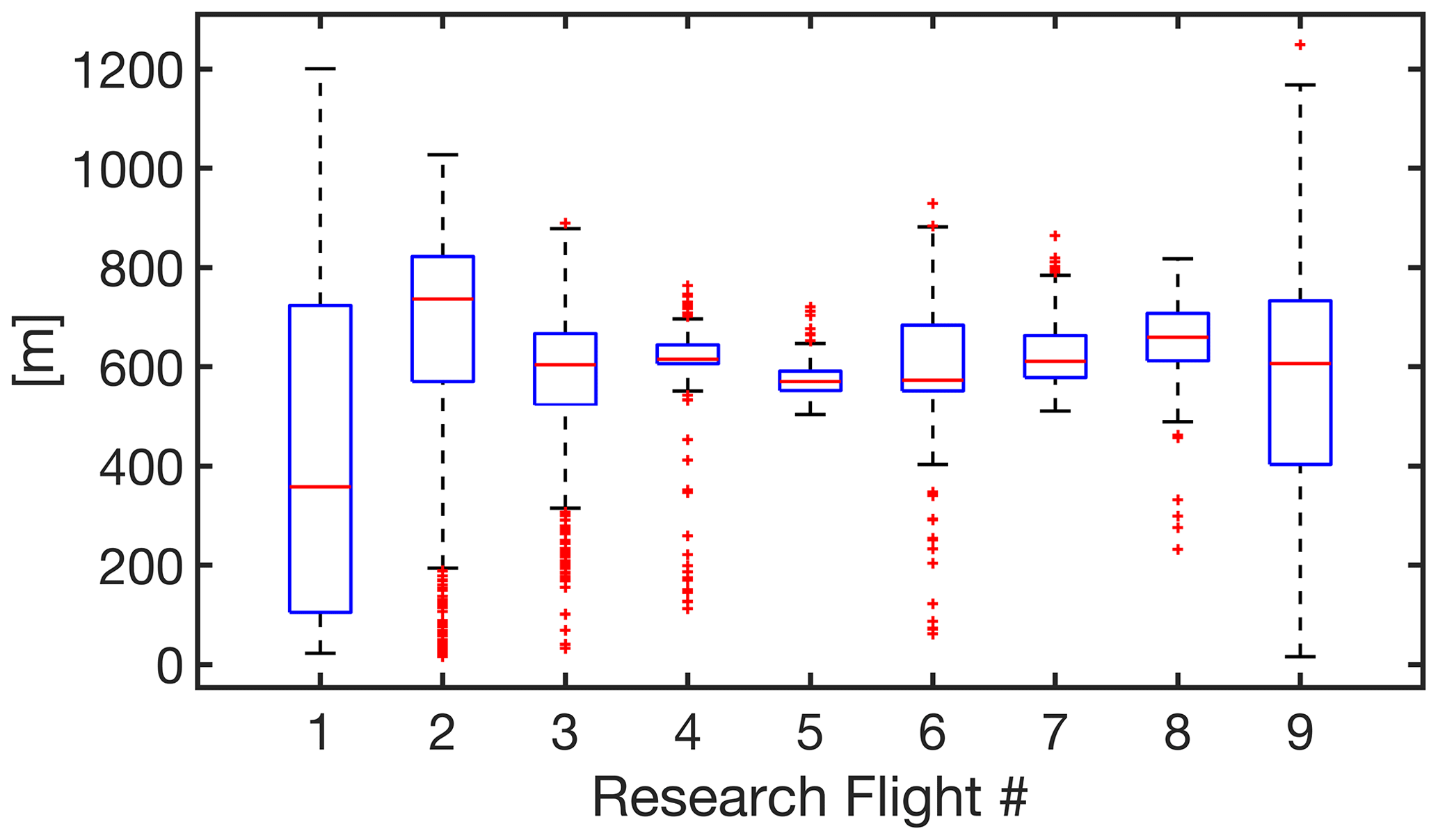
Figure 6The box–whisker plots of geolocation errors (avionics-only orthorectification data) before the corrections. These plots are based on the successful cases from GeoAKAZE. On each box, the central red line shows the median, and the top and bottom edges of the box show the 25th (q1) and 75th (q3) percentiles. The dark solid lines at the very beginning and the end of each plot show the minimum and maximum values. Red plus symbols indicate outliers that are determined by any value above or below .
An example of the offset is presented within Fig. 7a for O2 (background) and CH4 (foreground), respectively, where the radiance has been converted to grayscale units. This was done by averaging the radiance data in the wavelength ranges of 1602–1638 and 1245–1273 nm for the CH4 and O2 sensors, respectively, normalizing these averages to the maximum observed value in each, scaling by a factor of 255, and then applying the adaptive histogram equalization. Performing a full-physics retrieval on such data will not be possible where pixel [i,j] (in terms of along and across dimensions) of the O2 channel does not align with pixel [i,j] of the respective CH4 granule.
Approximate 30 s of L0 data streams are processed into smaller granules of 10 s, and in particular instances, it is possible that there is an offset along-track (number of frames) of respective CH4 and O2 granules. The offset along the track is very subtle, often fewer than one to two frames, but across the track the offset is large, evident from Fig. 7a and b.
To deduce the offset corrections, we leveraged the GeoAKAZE relative correction parameters to set a mesh grid of tie points having identical latitudes and longitudes between two channels. Because the relative correction has co-registered these two bands with respect to each other and this process is irrespective of the performance of the absolute correction, these tie points should be legitimate choices to co-register two images in the image domain. This approach also reduces the computational costs associated with running A-KAZE because it leverages the correction parameters made during the relative correction; thus, we are no longer required to recall A-KAZE. We identify the [i,j] of the tie points and estimate two offsets, i.e., the offset pixel numbers in each dimension. In Fig. 7b, the corrected CH4 grayscale image is shown. For this, an along-track shift of three frames and an across-track shift of 163 were deduced to match two images in the image space. In general, the across-track and along-track shifts were found to be 192±15 pixels and 1±1 pixels for RF01 and RF02. While the along-track offset remained the same for other flights, the across-track shift was reduced to 159±5 pixels due to the O2 camera being physically remounted onto the O2 after RF03.
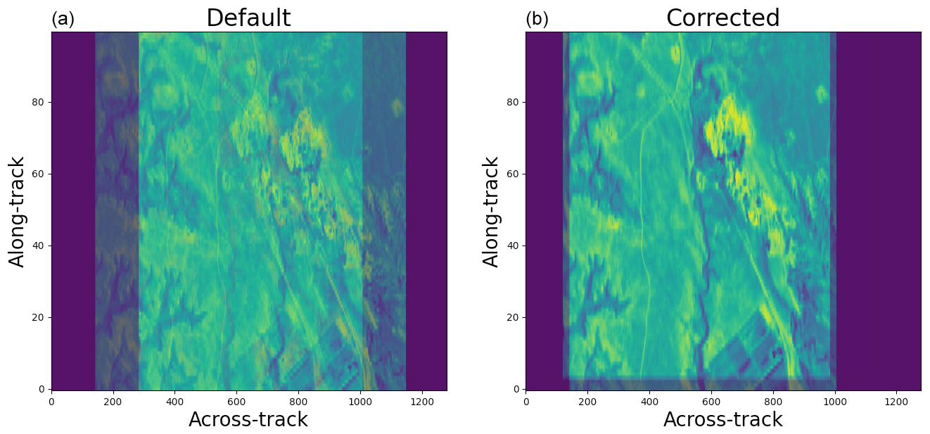
Figure 7An example of the alignment offsets in respectively time-stamped CH4 (foreground) and O2 (background) granules of 10 s in length, procured during RF08. (a) The original radiance images. (b) The overlaid and aligned CH4 and O2 radiance images.
3.9 Aggregation
The signal-to-noise ratio (SNR) for individual pixels at the native resolution is approximately 90 and 140 for the CH4 and O2 spectrometers, respectively, which can sometimes be too low for accurately performing retrieval studies. To address this, the native-resolution L1B files are supplemented with aggregated L1B data. We aggregated the native data into five segments of across-track pixels (5×1). By performing this, the SNR is boosted by a factor of 2.2 for a 5×1 aggregation.
The mission goal of MethaneSAT is to precisely map over 80 % of the production sources of methane emissions from oil and gas fields across the globe to an accuracy of 2–4 ppb on a 2 km2 scale. Accomplishing this task requires processing L0 data streams to L1B products with high accuracy. The MethaneAIR airborne simulator has provided critical science data to develop mature and efficient algorithms that will be utilized in the L0–L1B processor for MethaneSAT. Within the observation data of the MethaneAIR research flights, the development of several corrections was required.
Bad pixels are flagged by considering their standard deviation from the mean dark current, collected at numerous intervals throughout each flight. Stray light was corrected by following the results of Staebell et al. (2021), where a far-field kernel is utilized to redistribute light outside a 15 × 11 spectral–spatial window.
A forward model was developed using the latest available spectroscopic data from HITRAN2020. These were combined with a high-resolution solar spectrum and laboratory calibration data for both oxygen and methane sensors. A small increase in cabin temperature which occurred during the second research flight of MethaneAIR caused the instrument line shape to deviate from the laboratory-measured values; this became evident during wavelength calibration. The temperature increase was approximately 3–4 K. The forward model is demonstrated to accurately capture in-flight modulation of both the wavelength shift and ILS to a reasonable degree of accuracy.
To project MethaneAIR radiance observations onto the Earth’s surface (orthorectification), we trace light rays from the instrument through a camera model to the surface topography. The orthorectification procedure is subject to errors on the order of 600–800 m, primarily due to uncertainty in the position and attitude of the camera. The orientation of each spectrometer relative to the aircraft avionics system will be a consistent 3D rotation that can improve the accuracy of the initial first-guess derivation of the longitude and latitude of the L1B files. In future iterations, we will investigate this 3D correction to improve the efficiency of the L0–L1B processing. To correct these errors, we register MethaneAIR O2 band radiances to existing georeferenced MSI band 11 imagery using a fully automated feature extraction method called A-KAZE. We then apply the same algorithm to register MethaneAIR CH4 band radiances to MethaneAIR O2 band radiances. We then optimize the aircraft position and each camera’s attitude to best fit the registered data (reprojection). Surface features in the orthorectified images in both flights are well aligned, suggesting significant improvements in the geolocation accuracy for most scenes (>90 %). Nonetheless, we are aware of two important limitations of this approach, which are (i) the presence of cloud and (ii) a long lag between the acquisition time of MSI and MethaneAIR for some cases due to our stringent cloud-screening cut-off value, resulting in unmatchable key points. This automatic algorithm, called GeoAKAZE, is publicly available (Souri, 2022) and can be used for other airborne missions.
The misalignment of the radiance data recorded by the methane and oxygen sensors initially makes them unsuitable for use in full-physics retrieval algorithms, which requires the use of both channels. By converting the radiance data to grayscale images, we demonstrate via the use of the relative correction parameters made by the A-KAZE algorithm that the offsets (in pixel space) between the two sensors can be deduced to high accuracy and reliability. In this approach, the methane data were aligned to the oxygen sensor's data, and frames were added or subtracted to create a full matching set of data when necessary. This misalignment is expected to be much smaller for MethaneSAT.
The MethaneSAT L0–L1B processor will include all the algorithms described in this article, although not all may be required, and some may need to be modified.
EAC, AHS, JB, KS, CS, and BL developed scientific algorithms. JW, SR, CCM, and AC contributed to algorithm design. IG contributed to the spectroscopic data. JS, MS, JH, and BD provided expertise on instrument design. XL, JF, KL, and SW provided oversight on the campaign flight plans, algorithm designs, and overall project guidance.
The contact author has declared that none of the authors has any competing interests.
Publisher's note: Copernicus Publications remains neutral with regard to jurisdictional claims made in the text, published maps, institutional affiliations, or any other geographical representation in this paper. While Copernicus Publications makes every effort to include appropriate place names, the final responsibility lies with the authors.
This research was funded by MethaneSAT LLC and an NSF EAGER grant.
This paper was edited by Meng Gao and reviewed by three anonymous referees.
Alcantarilla, P., Nuevo, J., and Bartoli, A.: Fast Explicit Diffusion for Accelerated Features in Nonlinear Scale Spaces, in: Procedings of the British Machine Vision Conference 2013, Bristol, UK, 9–13 September 2013, British Machine Vision Association, https://doi.org/10.5244/c.27.13, 2013. a, b
Baiocchi, V., Giannone, F., Monti, F., and Vatore, F.: ACYOTB Plugin: Tool for Accurate Orthorectification in Open-Source Environments, ISPRS International J. Geo-Inf., 9, 11, https://doi.org/10.3390/ijgi9010011, 2020. a
Beirle, S., Lampel, J., Lerot, C., Sihler, H., and Wagner, T.: Parameterizing the instrumental spectral response function and its changes by a super-Gaussian and its derivatives, Atmos. Meas. Tech., 10, 581–598, https://doi.org/10.5194/amt-10-581-2017, 2017. a
Bertaux, J.-L., Hauchecorne, A., Lefèvre, F., Bréon, F.-M., Blanot, L., Jouglet, D., Lafrique, P., and Akaev, P.: The use of the 1.27 µm O2 absorption band for greenhouse gas monitoring from space and application to MicroCarb, Atmos. Meas. Tech., 13, 3329–3374, https://doi.org/10.5194/amt-13-3329-2020, 2020. a
Byrd, R. H., Lu, P., Nocedal, J., and Zhu, C.: A Limited Memory Algorithm for Bound Constrained Optimization, SIAM Journal on Scientific Computing, 16, 1190–1208, https://doi.org/10.1137/0916069, 1995. a
Cai, Z., Sun, K., Yang, D., Liu, Y., Yao, L., Lin, C., and Liu, X.: On-Orbit Characterization of TanSat Instrument Line Shape Using Observed Solar Spectra, Remote Sens., 14, 3334, https://doi.org/10.3390/rs14143334, 2022. a
Coddington, O. M., Richard, E. C., Harber, D., Pilewskie, P., Woods, T. N., Chance, K., Liu, X., and Sun, K.: The TSIS-1 Hybrid Solar Reference Spectrum, Geophys. Res. Lett., 48, e2020GL091709, https://doi.org/10.1029/2020GL091709, 2021. a
Drouin, B. J., Yu, S., Elliott, B. M., Crawford, T. J., and Miller, C. E.: High resolution spectral analysis of oxygen. III. Laboratory investigation of the airglow bands, J. Chem. Phys., 139, 144301, https://doi.org/10.1063/1.4821759, 2013. a
Drouin, B. J., Benner, D. C., Brown, L. R., Cich, M. J., Crawford, T. J., Devi, V. M., Guillaume, A., Hodges, J. T., Mlawer, E. J., Robichaud, D. J., Oyafuso, F., Payne, V. H., Sung, K., Wishnow, E. H., and Yu, S.: Multispectrum analysis of the oxygen A-band, J. Quant. Spectrosc. Ra., 186, 118–138, https://doi.org/10.1016/j.jqsrt.2016.03.037, 2017. a
Etheridge, D. M., Steele, L. P., Francey, R. J., and Langenfelds, R. L.: Atmospheric methane between 1000 A.D. and present: Evidence of anthropogenic emissions and climatic variability, J. Geophys. Res.-Atmos., 103, 15979–15993, https://doi.org/10.1029/98JD00923, 1998. a
Forster, P., Ramaswamy, V., Artaxo, P., Berntsen, T., Betts, R., Fahey, D., Haywood, J., Lean, J., Lowe, D., Myhre, G., Nganga, J., Prinn, R., Raga, G., Schulz, M., and Van Dorland, R.: Changes in Atmospheric Constituents and in Radiative Forcing, Climate Change 2007: The Physical Science Basis. Contribution of Working Group I to the Fourth Assessment Report of the IPCC, edited by: Solomon, S., Qin, D., and Manning, M., Cambridge University Press, Cambridge, UK, Chap. 2, http://www.cambridge.org/catalogue/catalogue.asp?isbn=9780521705967 (last access: 1 June 2022), 2008. a
Gerilowski, K., Tretner, A., Krings, T., Buchwitz, M., Bertagnolio, P. P., Belemezov, F., Erzinger, J., Burrows, J. P., and Bovensmann, H.: MAMAP – a new spectrometer system for column-averaged methane and carbon dioxide observations from aircraft: instrument description and performance analysis, Atmos. Meas. Tech., 4, 215–243, https://doi.org/10.5194/amt-4-215-2011, 2011. a
Gordon, I. E., Rothman, L. S., Hargreaves, R. J., Hashemi, R., Karlovets, E. V., Skinner, F. M., Conway, E. K., Hill, C., Kochanov, R. V., Tan, Y., Wcisło, P., Finenko, A. A., Nelson, K., Bernath, P. F., Birk, M., Boudon, V., Campargue, A., Chance, K. V., Coustenis, A., Drouin, B. J., Flaud, J.-M., Gamache, R. R., Hodges, J. T., Jacquemart, D., Mlawer, E. J., Nikitin, A. V., Perevalov, V. I., Rotger, M., Tennyson, J., Toon, G. C., Tran, H., Tyuterev, V. G., Adkins, E. M., Baker, A., Barbe, A., Canè, E., Császár, A. G., Dudaryonok, A., Egorov, O., Fleisher, A. J., Fleurbaey, H., Foltynowicz, A., Furtenbacher, T., Harrison, J. J., Hartmann, J.-M., Horneman, V.-M., Huang, X., Karman, T., Karns, J., Kassi, S., Kleiner, I., Kofman, V., Kwabia-Tchana, F., Lavrentieva, N. N., Lee, T. J., Long, D. A., Lukashevskaya, A. A., Yulin, O. M., Makhnev, V. Y., Matt, W., Massie, S. T., Melosso, M., Mikhailenko, S. N., Mondelain, D., Müller, H. S. P., Naumenko, O. V., Perrin, A., Polyansky, O. L., Raddaoui, E., Raston, P. L., Reed, Z. D., Rey, M., Richard, C., Tóbiás, R., Sadiek, I., Schwenke, D. W., Starikova, E., Sung, K., Tamassia, F., Tashkun, S. A., Auwera, J. V., Vasilenko, I. A., Vigasin, A. A., Villanueva, G. L., Vispoel, B., Wagner, G., Yachmenev, A., and Yurchenko, S. N.: The HITRAN2020 molecular spectroscopic database, J. Quant. Spectrosc. Ra., 277, 107949, https://doi.org/10.1016/j.jqsrt.2021.107949, 2021. a
Hmiel, B., Petrenko, V. V., Dyonisius, M. N., Buizert, C., Smith, A. M., Place, P. F., Harth, C., Beaudette, R., Hua, Q., Yang, B., Vimont, I., Michel, S. E., Severinghaus, J. P., Etheridge, D., Bromley, T., Schmitt, J., Faïn, X., Weiss, R. F., and Dlugokencky, E.: Preindustrial 14CH4 indicates greater anthropogenic fossil CH4 emissions, Nature, 578, 409–412, https://doi.org/10.1038/s41586-020-1991-8, 2020. a
Humpage, N., Boesch, H., Palmer, P. I., Vick, A., Parr-Burman, P., Wells, M., Pearson, D., Strachan, J., and Bezawada, N.: GreenHouse gas Observations of the Stratosphere and Troposphere (GHOST): an airborne shortwave-infrared spectrometer for remote sensing of greenhouse gases, Atmos. Meas. Tech., 11, 5199–5222, https://doi.org/10.5194/amt-11-5199-2018, 2018. a
Karman, T., Koenis, M. A. J., Banerjee, A., Parker, D. H., Gordon, I. E., van der Avoird, A., van der Zande, W. J., and Groenenboom, G. C.: O2−O2 and O2−N2 collision-induced absorption mechanisms unravelled, Nat. Chem., 10, 549–554, https://doi.org/10.1038/s41557-018-0015-x, 2018. a
Karman, T., Gordon, I. E., van der Avoird, A., Baranov, Y. I., Boulet, C., Drouin, B. J., Groenenboom, G. C., Gustafsson, M., Hartmann, J.-M., Kurucz, R. L., Rothman, L. S., Sun, K., Sung, K., Thalman, R., Tran, H., Wishnow, E. H., Wordsworth, R., Vigasin, A. A., Volkamer, R., and van der Zande, W. J.: Update of the HITRAN collision-induced absorption section, Icarus, 328, 160–175, https://doi.org/10.1016/j.icarus.2019.02.034, 2019. a
Kleipool, Q., Ludewig, A., Babić, L., Bartstra, R., Braak, R., Dierssen, W., Dewitte, P.-J., Kenter, P., Landzaat, R., Leloux, J., Loots, E., Meijering, P., van der Plas, E., Rozemeijer, N., Schepers, D., Schiavini, D., Smeets, J., Vacanti, G., Vonk, F., and Veefkind, P.: Pre-launch calibration results of the TROPOMI payload on-board the Sentinel-5 Precursor satellite, Atmos. Meas. Tech., 11, 6439–6479, https://doi.org/10.5194/amt-11-6439-2018, 2018. a
Konefał, M., Kassi, S., Mondelain, D., and Campargue, A.: High sensitivity spectroscopy of the O2 band at 1.27 µm: (I) pure O2 line parameters above 7920 cm−1, J. Quant. Spectrosc. Ra., 241, 1–12, https://doi.org/10.1016/j.jqsrt.2019.106653, 2020. a
Kowalewski, M. G. and Janz, S. J.: Remote sensing capabilities of the Airborne Compact Atmospheric Mapper, Proc. SPIE 7452, Earth Observing Systems XIV, 74520Q, 225–234, https://doi.org/10.1117/12.827035, 2009. a
Kuze, A., Suto, H., Shiomi, K., Kataoka, F., Kawashima, T., Oda, T., Fujinawa, T., Kanaya, Y., and Tanimoto, H.: City-level CO2, CH4, and NO2 observations from Space: Airborne model demonstration over Nagoya, Earth and Space Science Open Archive [preprint], https://doi.org/10.1002/essoar.10502004.1, 2020. a
Lamsal, L. N., Janz, S. J., Krotkov, N. A., Pickering, K. E., Spurr, R. J. D., Kowalewski, M. G., Loughner, C. P., Crawford, J. H., Swartz, W. H., and Herman, J. R.: High-resolution NO2 observations from the Airborne Compact Atmospheric Mapper: Retrieval and validation, J. Geophys. Res.-Atmos., 122, 1953–1970, https://doi.org/10.1002/2016JD025483, 2017. a
Leitch, J. W., Delker, T., Good, W., Ruppert, L., Murcray, F., Chance, K., Liu, X., Nowlan, C., Janz, S. J., Krotkov, N. A., Pickering, K. E., Kowalewski, M., and Wang, J.: The GeoTASO airborne spectrometer project, Proc. SPIE 9218, Earth Observing Systems XIX, 92181H, 487–495, https://doi.org/10.1117/12.2063763, 2014. a
Liu, C., Liu, X., Kowalewski, M. G., Janz, S. J., González Abad, G., Pickering, K. E., Chance, K., and Lamsal, L. N.: Characterization and verification of ACAM slit functions for trace-gas retrievals during the 2011 DISCOVER-AQ flight campaign, Atmos. Meas. Tech., 8, 751–759, https://doi.org/10.5194/amt-8-751-2015, 2015. a
Maté, B., Lugez, C., Fraser, G. T., and Lafferty, W. J.: Absolute intensities for the O2 1.27 µm continuum absorption, J. Geophys. Res.-Atmos., 104, 30585–30590, https://doi.org/10.1029/1999JD900824, 1999. a
MethaneSAT LLC: MethaneSAT, https://www.methanesat.org/fit-with-other-missions/, last access: 16 March 2021. a
Miller, C. E. and Wunch, D.: Fourier transform spectrometer remote sensing of O2 A-band electric quadrupole transitions, J. Quant. Spectrosc. Ra., 113, 1043–1050, https://doi.org/10.1016/j.jqsrt.2012.01.002, 2012. a
NCAR – Earth Observing Laboratory: NSF/NCAR GV HIAPER Aircraft, UCAR/NCAR – Earth Observing Laboratory [data set], https://doi.org/10.5065/D6DR2SJP, 2005. a
Nisbet, E. G., Manning, M. R., Dlugokencky, E. J., Fisher, R. E., Lowry, D., Michel, S. E., Myhre, C. L., Platt, S. M., Allen, G., Bousquet, P., Brownlow, R., Cain, M., France, J. L., Hermansen, O., Hossaini, R., Jones, A. E., Levin, I., Manning, A. C., Myhre, G., Pyle, J. A., Vaughn, B. H., Warwick, N. J., and White, J. W. C.: Very Strong Atmospheric Methane Growth in the 4 Years 2014–2017: Implications for the Paris Agreement, Global Biogeochem. Cy., 33, 318–342, https://doi.org/10.1029/2018GB006009, 2019. a
NOAA: Despite pandemic shutdowns, carbon dioxide and methane surged in 2020, https://research.noaa.gov/article/ArtMID/587/ ArticleID/2742/Despite-pandemic-shutdowns-carbon-dioxide-and-methane-surged-in-2020 (last access: 22 April 2021), 2021. a
Nowlan, C. R., Liu, X., Leitch, J. W., Chance, K., González Abad, G., Liu, C., Zoogman, P., Cole, J., Delker, T., Good, W., Murcray, F., Ruppert, L., Soo, D., Follette-Cook, M. B., Janz, S. J., Kowalewski, M. G., Loughner, C. P., Pickering, K. E., Herman, J. R., Beaver, M. R., Long, R. W., Szykman, J. J., Judd, L. M., Kelley, P., Luke, W. T., Ren, X., and Al-Saadi, J. A.: Nitrogen dioxide observations from the Geostationary Trace gas and Aerosol Sensor Optimization (GeoTASO) airborne instrument: Retrieval algorithm and measurements during DISCOVER-AQ Texas 2013, Atmos. Meas. Tech., 9, 2647–2668, https://doi.org/10.5194/amt-9-2647-2016, 2016. a
Nowlan, C. R., Liu, X., Janz, S. J., Kowalewski, M. G., Chance, K., Follette-Cook, M. B., Fried, A., González Abad, G., Herman, J. R., Judd, L. M., Kwon, H.-A., Loughner, C. P., Pickering, K. E., Richter, D., Spinei, E., Walega, J., Weibring, P., and Weinheimer, A. J.: Nitrogen dioxide and formaldehyde measurements from the GEOstationary Coastal and Air Pollution Events (GEO-CAPE) Airborne Simulator over Houston, Texas, Atmos. Meas. Tech., 11, 5941–5964, https://doi.org/10.5194/amt-11-5941-2018, 2018. a
Pandey, S., Gautam, R., Houweling, S., van der Gon, H. D., Sadavarte, P., Borsdorff, T., Hasekamp, O., Landgraf, J., Tol, P., van Kempen, T., Hoogeveen, R., van Hees, R., Hamburg, S. P., Maasakkers, J. D., and Aben, I.: Satellite observations reveal extreme methane leakage from a natural gas well blowout, P. Natl. Acad. Sci. USA, 116, 26376–26381, https://doi.org/10.1073/pnas.1908712116, 2019. a
Souri, A. H.: GEOAkaze, Zenodo [code], https://doi.org/10.5281/zenodo.6993473, 2022. a, b, c
Staebell, C., Sun, K., Samra, J., Franklin, J., Chan Miller, C., Liu, X., Conway, E., Chance, K., Milligan, S., and Wofsy, S.: Spectral calibration of the MethaneAIR instrument, Atmos. Meas. Tech., 14, 3737–3753, https://doi.org/10.5194/amt-14-3737-2021, 2021. a, b, c, d, e, f, g, h, i, j
Sun, K., Liu, X., Huang, G., González Abad, G., Cai, Z., Chance, K., and Yang, K.: Deriving the slit functions from OMI solar observations and its implications for ozone-profile retrieval, Atmos. Meas. Tech., 10, 3677–3695, https://doi.org/10.5194/amt-10-3677-2017, 2017a. a
Sun, K., Liu, X., Nowlan, C. R., Cai, Z., Chance, K., Frankenberg, C., Lee, R. A. M., Pollock, R., Rosenberg, R., and Crisp, D.: Characterization of the OCO-2 instrument line shape functions using on-orbit solar measurements, Atmos. Meas. Tech., 10, 939–953, https://doi.org/10.5194/amt-10-939-2017, 2017b. a, b
Sun, K., Gordon, I. E., Sioris, C. E., Liu, X., Chance, K., and Wofsy, S. C.: Reevaluating the Use of O2 a1 Δg Band in Spaceborne Remote Sensing of Greenhouse Gases, Geophys. Res. Lett., 45, 5779–5787, https://doi.org/10.1029/2018GL077823, 2018. a
Thompson, D. R., Thorpe, A. K., Frankenberg, C., Green, R. O., Duren, R., Guanter, L., Hollstein, A., Middleton, E., Ong, L., and Ungar, S.: Space-based remote imaging spectroscopy of the Aliso Canyon CH4 superemitter, Geophys. Res. Lett., 43, 6571–6578, https://doi.org/10.1002/2016GL069079, 2016. a
Tol, P. J. J., van Kempen, T. A., van Hees, R. M., Krijger, M., Cadot, S., Snel, R., Persijn, S. T., Aben, I., and Hoogeveen, R. W. M.: Characterization and correction of stray light in TROPOMI-SWIR, Atmos. Meas. Tech., 11, 4493–4507, https://doi.org/10.5194/amt-11-4493-2018, 2018. a
Tran, D., Tran, H., Vasilchenko, S., Kassi, S., Campargue, A., and Mondelain, D.: High sensitivity spectroscopy of the O2 band at 1.27 µm: (II) air-broadened line profile parameters, J. Quant. Spectrosc. Ra., 240, 106673, https://doi.org/10.1016/j.jqsrt.2019.106673, 2020. a
Turner, A. J., Frankenberg, C., and Kort, E. A.: Interpreting contemporary trends in atmospheric methane, P. Natl. Acad. Sci. USA, 116, 2805–2813, https://doi.org/10.1073/pnas.1814297116, 2019. a
van Hees, R. M., Tol, P. J. J., Cadot, S., Krijger, M., Persijn, S. T., van Kempen, T. A., Snel, R., Aben, I., and Hoogeveen, Ruud W. M.: Determination of the TROPOMI-SWIR instrument spectral response function, Atmos. Meas. Tech., 11, 3917–3933, https://doi.org/10.5194/amt-11-3917-2018, 2018. a
van Kempen, T. A., van Hees, R. M., Tol, P. J. J., Aben, I., and Hoogeveen, R. W. M.: In-flight calibration and monitoring of the Tropospheric Monitoring Instrument (TROPOMI) short-wave infrared (SWIR) module, Atmos. Meas. Tech., 12, 6827–6844, https://doi.org/10.5194/amt-12-6827-2019, 2019. a
Veefkind, J., Aben, I., McMullan, K., Förster, H., de Vries, J., Otter, G., Claas, J., Eskes, H., de Haan, J., Kleipool, Q., van Weele, M., Hasekamp, O., Hoogeveen, R., Landgraf, J., Snel, R., Tol, P., Ingmann, P., Voors, R., Kruizinga, B., Vink, R., Visser, H., and Levelt, P.: TROPOMI on the ESA Sentinel-5 Precursor: A GMES mission for global observations of the atmospheric composition for climate, air quality and ozone layer applications, Remote Sens. Environ., 120, 70–83, https://doi.org/10.1016/j.rse.2011.09.027, 2012. a
Voors, R., Dobber, M., Dirksen, R., and Levelt, P.: Method of calibration to correct for cloud-induced wavelength shifts in the Aura satellite's Ozone Monitoring Instrument, Appl. Optics, 45, 3652–3658, https://doi.org/10.1364/AO.45.003652, 2006. a
Zhang, H., Zheng, G., and Fu, H.: Research on Image Feature Point Matching Based on ORB and RANSAC Algorithm, J. Phys. Conf. Ser., 1651, 012187, https://doi.org/10.1088/1742-6596/1651/1/012187, 2020. a
Zhang, Y., Gautam, R., Pandey, S., Omara, M., Maasakkers, J. D., Sadavarte, P., Lyon, D., Nesser, H., Sulprizio, M. P., Varon, D. J., Zhang, R., Houweling, S., Zavala-Araiza, D., Alvarez, R. A., Lorente, A., Hamburg, S. P., Aben, I., and Jacob, D. J.: Quantifying methane emissions from the largest oil-producing basin in the United States from space, Sci. Adv., 6, eaaz5120, https://doi.org/10.1126/sciadv.aaz5120, 2020. a
Zoogman, P., Liu, X., Suleiman, R. M., Pennington, W. F., Flittner, D. E., Al-Saadi, J. A., Hilton, B. B., Nicks, D. K., Newchurch, M. J., Carr, J. L., Janz, S. J., Andraschko, M. R., Arola, A., Baker, B. D., Canova, B. P., Miller, C. C., Cohen, R. C., Davis, J. E., Dussault, M. E., Edwards, D. P., Fishman, J., Ghulam, A., Abad, G. G., Grutter, M., Herman, J. R., Houck, J., Jacob, D. J., Joiner, J., Kerridge, B. J., Kim, J., Krotkov, N. A., Lamsal, L., Li, C., Lindfors, A., Martin, R. V., McElroy, C. T., McLinden, C., Natraj, V., Neil, D. O., Nowlan, C. R., O'Sullivan, E. J., Palmer, P. I., Pierce, R. B., Pippin, M. R., Saiz-Lopez, A., Spurr, R. J. D., Szykman, J. J., Torres, O., Veefkind, J. P., Veihelmann, B., Wang, H., Wang, J., and Chance, K.: Tropospheric emissions: Monitoring of pollution (TEMPO), J. Quant. Spectrosc. Ra., 186, 17–39, https://doi.org/10.1016/j.jqsrt.2016.05.008, 2017. a