the Creative Commons Attribution 4.0 License.
the Creative Commons Attribution 4.0 License.
 | 08 Mar 2024
Modelling of cup anemometry and dynamic overspeeding in average wind speed measurements
Troels Friis Pedersen
Jan-Åke Dahlberg
Cup anemometers measure average wind speed in the atmosphere and have been used for one and a half centuries by meteorologists. Within the last half century, cup anemometers have been used extensively in wind energy to measure wind resources and performance of wind turbines. Meteorologists researched cup anemometer behaviour and found dynamic overspeeding to be an inherent and significant systematic error. The wind energy community has strong accuracy requirements for power performance measurements on wind turbines, and this led in the last 2 decades to new research on cup anemometer characteristics, which was taken to a new level with the development of improved calibration procedures, cup anemometer calculation models and classification methods.
Research projects in wind energy demonstrated, by field and wind tunnel measurements, that angular response was a significant contributor to uncertainty and that dynamic overspeeding was a significant but less important contributor. Earlier research was mainly made on cup anemometers with hemispherical cups on long arms, and dynamic overspeeding was considered an inherent and high uncertainty error for cup anemometers. Research on conical cups on short arms has now shown that zero or low overspeeding is present on a well-designed cup anemometer, providing a much lower overspeeding uncertainty error. Different cup anemometer calculation models were investigated in order to find derived overspeeding characteristics. The general and often used parabolic torque coefficient model showed that zero overspeeding is present when the speed ratio roots of the torque coefficient curve go through the equilibrium speed ratio and zero. The two-cup drag model is a special case of the parabolic torque coefficient model but with the second root being reciprocal to the equilibrium speed ratio. The drag model always results in a positive maximum overspeeding of the order of 1.1 times the turbulence intensity squared. A linear torque coefficient results in maximum overspeeding levels equal to the turbulence intensity squared. Torque characteristics of a cup anemometer with hemispherical cups fit slightly well to the drag model, but a cup anemometer with conical cups does not fit to the drag model nor the parabolic model; it fits better to a partial linear model and even better to an optimized torque model. The most accurate modelling of cup anemometer characteristics is at present made with the ACCUWIND model (Dahlberg et al., 2006). This model uses tabulated torque coefficient and angular response data measured in a wind tunnel. The ACCUWIND model is found in International Electrotechnical Commission (IEC) wind turbine power performance standards, where it is used in a classification system for estimation of operational uncertainties. For an actual comparison of two cup anemometers, with respectively hemispherical and conical cups, the influence of dynamic overspeeding was found to be relatively low compared to angular response, but for conical cups it was specifically low.
- Article
(2864 KB) - Full-text XML
- BibTeX
- EndNote


Cup anemometry has, since about 1980, been used intensively in the wind energy community to assess wind resources and to document wind turbine power curves. A strong trust to this simple instrument was due to a long history in meteorological measurements. A cup anemometer consists of a vertical shaft with cup-shaped “cups” mounted on the top to provide rotation in the wind. John Thomas Romney Robinson was known to be the first to develop a cup anemometer with four hemispherical cups and to bring it into general use in 1846. The cup anemometer instrument was, however, suggested by Edgeworth many years before (Cleveland, 1888; Waldo, 1893). At the end of the 19th century, meteorological offices researched “the factor”, i.e. the gain calibration value, with swirling machines. These machines were set to rotate with a long horizontal arm with a cup anemometer mounted at the outer end. The meteorologists investigated the influence of the cup radius to rotor arm radius in order to determine the factor, i.e. the cup speed relative to the wind speed. Robinson developed a theory on the factor, which deviated, however, from other investigations with swirling machines and with outdoor cup anemometer comparisons (Cleveland, 1888; Waldo, 1893). Recently, Sanz-Andrés et al. (2014) investigated the factor with a number of different conical cup designs, cup sizes and cup arms. Sanz-Andrés et al. (2014) presented a thorough overview of literature on cup anemometry divided into different categories of research in the same article. In the 20th century, many meteorologists studied the overspeeding effect, i.e. a tendency to measure a higher average wind speed in fluctuating wind. With minor effort, they studied angular characteristics, i.e. the influence due to non-horizontal inflow angles. Despite the research made by meteorologists, the World Meteorological Organization has not over time presented strong requirements on accuracy of wind speed measurements with cup anemometers in their reports. Since 1980 and up until 2014, the requirement was 0.5 m s−1 below 5 m s−1 and 10 % above 5 m s−1 (WMO, 2014). The wind energy community made, from the start, use of the research made by the meteorologists, but it was found that stronger requirements on measurement accuracy were needed. The community was forced to make its own research and development on cup anemometry.
The wind energy community started intensely to measure wind turbine power curves (relation between free wind speed and wind turbine power output) with cup anemometers in the early 1980s. European wind turbine test stations met regularly to discuss common issues, especially challenges with power curve measurements and certification of wind turbines. This led to a European Joint Wind Turbine Test Station Programme to develop common procedures. The European test stations used different types of cup anemometers for power curve measurements and wind resource measurements. They calibrated the instruments in different types of wind tunnels with different procedures. An inter-calibration between the wind tunnels revealed in 1989 an up to 11 % difference in calibration of the same cup anemometer (Hunter, 1989a). The cooperation led to common requirements for use of cup anemometry and wind tunnel calibrations (Hunter, 1989b) and also to regular inter-calibrations. After years of improvement in procedures, harmonized and recognized measurements were set up in 1997 by MEASNET, a measurement organization implemented by the European test stations (MEASNET, 2023). Today, MEASNET perform regular inter-calibrations with the goal of less than 0.5 % differences in calibrations between the participating wind tunnels. All calibration institutes are accredited and are able to trace calibrations and uncertainties back to fundamental physical units.
Also in 1989, Barton (1989) discovered different dynamic behaviour in step responses (sudden increase or decrease in wind speed). From step responses, Barton determined the distance constant, defined as the distance the air flows past a cup anemometer during the time it takes the cup rotor to reach 63.2 % of the equilibrium speed after a step change in wind speed. Barton used the Meteorology Office Handbook (HMSO, 1981) as a reference. The distance constant definition is the same in the updated standard (ASTM, 2017). Barton determined distance constants of five instruments used by the European test stations, among them a Risø P2445b cup anemometer with conical cups and a Thies Classic cup anemometer with hemispherical cups. Barton reported distance constants for Risø of 2.8 and 2.1 m for increasing and decreasing steps, respectively. For Thies, Barton reported distance constants of 5.2 and 5.3 m, respectively. MacCready (1965) introduced the distance constant concept already in 1965, assuming that the distance constant was a fundamental instrument constant. With the step response measurements, Barton (1989) found evidence that the distance constant varied with the conditions, and it did not seem to be a fundamental constant. But at the time the implications were not studied further.
The recommendation on the use of cup anemometry (Hunter, 1989b) was followed up 10 years later by the IEA (International Energy Agency) by improved recommended practices (Hunter et al., 1999), a document that was widely used in wind energy. However, the IEA recommendation did not solve the problems of differences in power performance measurements experienced in field measurements with different types of cup anemometers. The experienced differences in wind speed measurements led to a European trade barrier between Germany and Denmark. Although accredited power curves were made in Denmark with Risø cup anemometers, when exporting wind turbines to Germany it was required that power curves were measured in Germany with Thies cup anemometers. Albers et al. (2001) sketched up the situation and described the dawning need of a classification system for cup anemometer performance in order to consider operational uncertainties, and in the SITEPARIDEN project they published differences in field comparisons between cup anemometers, among them the Risø and Thies cup anemometers (Albers, 2001). A procedure for classification of cup anemometers was proposed earlier (Pedersen and Paulsen, 1997). The procedure made use of the two-cup drag model introduced by Schrenk (1929). The procedure was further developed (Pedersen and Paulsen, 1999), and classifications of five commercial cup anemometers with the method were presented.
The definition of the preferred measured wind speed was also an issue. Not having a specific wind speed definition would alone provide for an uncertainty of 1.9 % at 20 % turbulence intensity by the available wind speed definitions (horizontal, vector, scalar) (Pedersen et al., 1996). An analysis of wind turbine output power in relation to the wind indicated that the 10 min vector–scalar averaged wind speed would be a suitable definition. The European CLASSCUP project (Dahlberg et al., 2001) was initiated to develop an optimum vector-average design of a cup anemometer and to prepare a classification system to allow users to select an anemometer suited to specific requirements and to assess operational uncertainties. The result of the CLASSCUP project was a cup anemometer design with a flat angular response but, unfortunately, also with relatively high overspeeding. A revised classification system was also proposed, using tabulated torque coefficient data in modelling instead of using fitted data to the drag or parabolic torque coefficient models. An example classification report was made on the Risø cup anemometer (Pedersen, 2004).
Further studies of the wind speed definition, where flow inclination angles for both cup anemometers and wind turbine blades were assessed, concluded that the most suitable definition of measured wind speed for power performance measurements was the 10 min average horizontal scalar wind speed (Pedersen, 2004). For cup anemometry, the horizontal wind speed definition is also the most obvious, due to the vertical shaft and the cosine relationship to the tilted flow. The European ACCUWIND project (Dahlberg et al., 2006) continued the research on cup anemometry with the horizontal-wind-speed definition. The horizontal-wind-speed definition was confirmed to be preferable over the vector definition (Eecen et al., 2006), largely due to the fact that wind turbines also respond to inflow angles with a cosine function but to a power of 2 to 4. The testing methods on cup anemometry were investigated for robustness, and the classification procedure was fine-tuned (Dahlberg et al., 2006). Five commercial cup anemometers were tested with the so-called ACCUWIND classification method (Pedersen et al., 2006). Included in these tests was an improved Thies cup anemometer with conical cups (Thies First Class).
The classification method was adopted in the IEC power performance measurement standard (IEC-12-1, 2005) in annexes I and J. The classification system is a method to assess the operational uncertainties in field measurements, Class A for flat terrain, Class B for complex terrain, and a Class S for arbitrary terrain and measurement conditions. Classes A and B are appropriate for selection of cup anemometry for measurement campaigns, while Class S is appropriate for uncertainty assessment of specific measurement campaigns. The IEC standard provides methods to combine the operational uncertainty of a cup anemometer with all other uncertainties with use of the uncertainty standard, later updated to BIPM (2008). The IEC classification method was continued in the revised standard (IEC-12-1, 2017), where cold climate Classes C to D were added. MEASNET institutes (members of the MEASNET organization) provide accredited calibration as well as classification of cup anemometers according to the IEC standard. The 2017 IEC standard was lately restructured into the power performance standard (IEC-12, 2022), which references the new measurement standard (IEC-50-1, 2022) to where cup anemometry was transferred.
The classification method requires use of an appropriate cup anemometer model to simulate the systematic deviations when taking the cup anemometer from the wind tunnel to the field. The cup anemometer model has to simulate field conditions but also the calibration conditions from where traceability is transferred, and the model must fit well to the calibration constants. The ACCUWIND model, the example model in the IEC standard, is a generic time-domain model that simulates the response of a cup anemometer exposed to 3D wind, using tabulated data of torque, angular response and bearing friction. Simpler models with mathematical expressions for torque characteristics do not describe the characteristics of actual cup anemometers to a sufficient detail, and they are therefore less useful for classification purposes. The mathematical models, however, imply dynamic characteristics, which are useful in the assessment of the overspeeding effect. These models are investigated in detail in the following sections.
Two actual cup anemometer types are used to demonstrate the range of characteristics of cup anemometer types, found in both field comparisons and in laboratory tests (see Fig. 1). The types are the previously mentioned Risø P2445b (similar to Risø P2546 in geometry and characteristics and only called Risø in the following) and the Thies 4.3303.22.000 (often called Thies Classic and only called Thies in the following). The Risø cup anemometer has three conical 70 mm diameter cups, and the radius from shaft centre to cup centre is 58 mm. The Thies cup anemometer has three hemispherical 79 mm diameter cups, and the radius from shaft centre to cup centre is 120 mm.
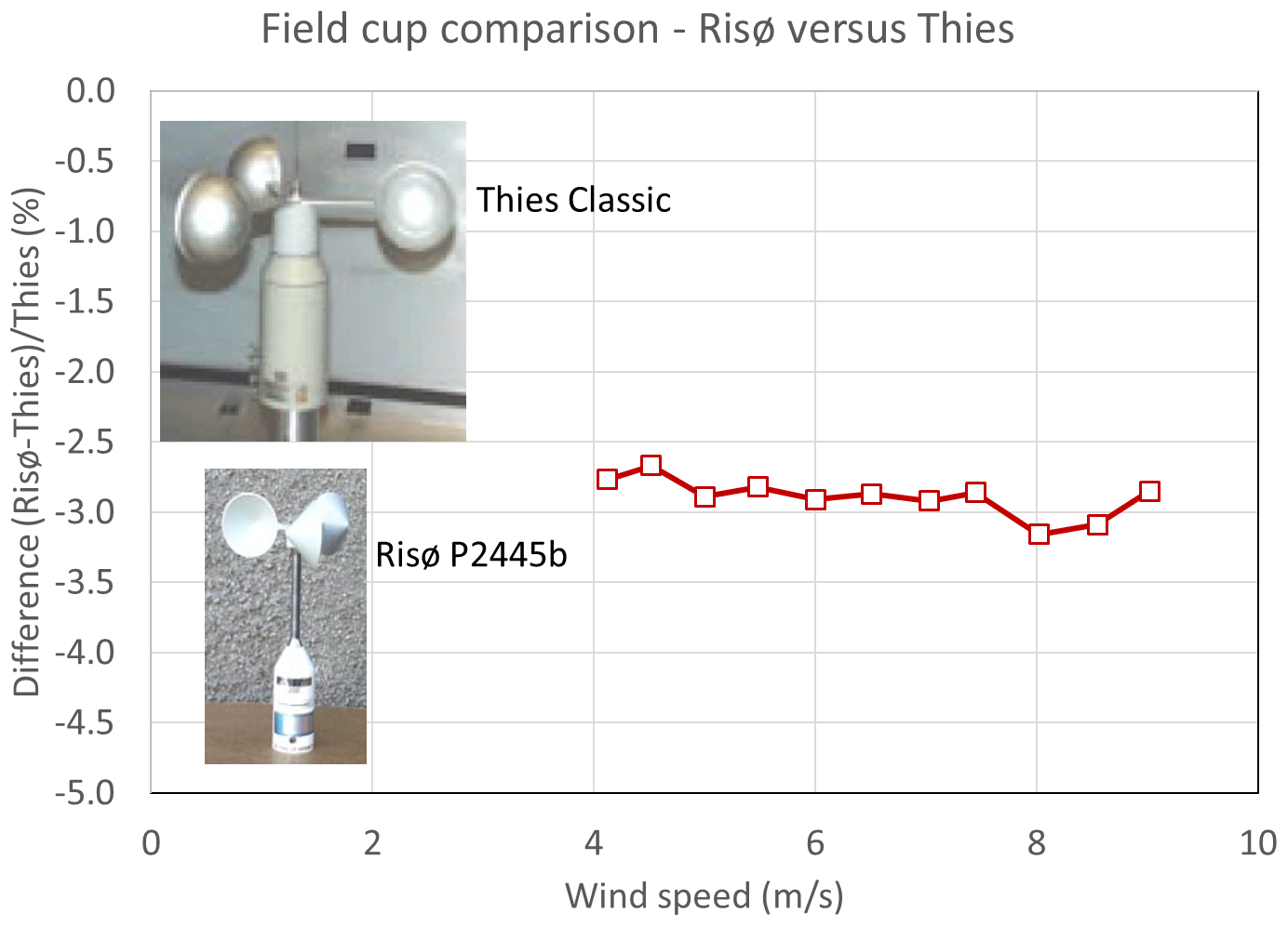
Figure 1Differences between Risø cup anemometer relative to Thies in a field comparison at a measurement height of 8 m; data are from SITEPARIDEN (Albers, 2001).
In the European SITEPARIDEN project, Albers (Albers, 2001), where he compared several cup anemometers in an experimental field set-up, found systematically 3 % lower values by the Risø cup anemometer compared to the Thies cup anemometer (see Fig. 1). The cup anemometers were calibrated in the same wind tunnel at the same time, so the differences were due to climatic influence parameters on the cup anemometers. Pedersen et al. (2002) made another field comparison experiment and found a significant systematic influence of turbulence between the Risø and Thies cup anemometers (see Fig. 2). The field experiments verified the high influence of especially turbulence on cup anemometer measurements. Papadopoulos et al. (2001) made yet another field comparison project. Five cup anemometers were compared in horizontal flow and also flow in tilted position. They observed up to 2 % differences at 12 % turbulence intensity and concluded that differences could not be explained by distance constant values alone (ranging from 1.7 to 5 m). The distance constant was in the IEA recommendation (Hunter et al., 1999) considered an important parameter to indicate the influence of dynamic overspeeding.
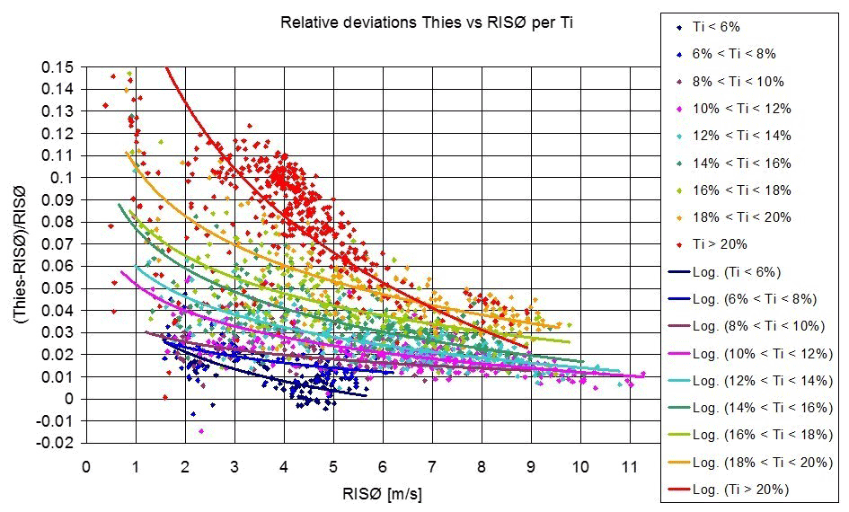
Figure 2Differences between Thies cup anemometer relative to Risø as a function of turbulence intensity (Ti), in a field comparison, from Pedersen et al. (2002).
By field experiments, the differences were discovered to be caused mainly by angular response, torque characteristics and bearing friction. Bearings on cup anemometer rotors are lubricated with oil or grease, which is sensitive to temperature. At lower temperatures, bearing friction increases and cup anemometers tend to measure lower wind speeds because of lower rotational speed. Fabian (1995) demonstrated a flywheel test method in a climate chamber to assess bearing friction, and he found significant friction differences between cup anemometer types. His method was adopted in the IEC standard (IEC-12-1, 2005). Optimum bearing friction is obviously zero friction or that friction is insensitive to temperature. Cup anemometers are calibrated at indoor temperatures but are used in field measurements, often at quite low temperatures. Temperature is thus an important influential parameter that is not to be neglected in field measurement uncertainty.
Turbulence is the most dominating influence parameter, as demonstrated in Fig. 2. The turbulent wind gives rise to instantaneous variations in upflow angle to the cup rotor. Wind tunnel calibration is made at horizontal flow, so the upflow angle gives rise to an aerodynamic response due to non-horizontal angles. Angular response was studied in detail by Westermann and Dahlberg in the CLASSCUP project (Dahlberg et al., 2001). Westermann made field tests of commercial cup anemometers in tilted configurations, and Dahlberg made wind tunnel tests on commercial cup anemometers as well as several potential designs for optimum flat angular response characteristics. Actual angular responses are generally not cosine shaped, and they cannot easily be represented by mathematical formulas. Tabulated data were found to be most accurate when used for cup anemometer classification. Several angular response characteristics for various cup anemometer configurations are reported in Dahlberg et al. (2001). Angular responses of the Thies and Risø cup anemometers are shown in Fig. 3.
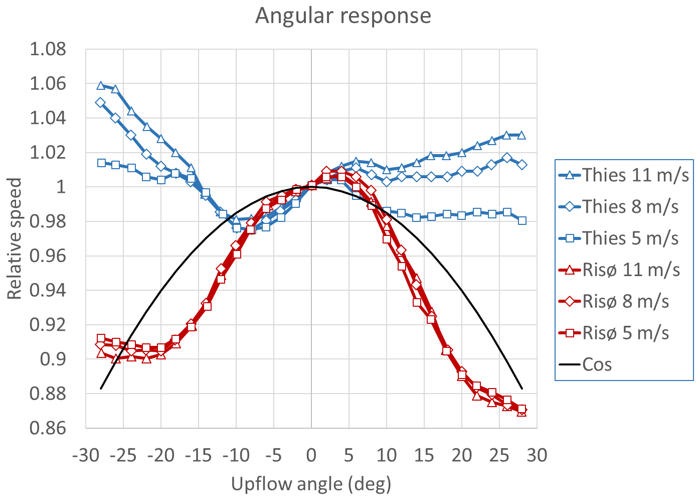
Figure 3Angular response of Thies and Risø cup anemometers. Measurement data are from Dahlberg et al. (2001).
Dynamic overspeeding is another turbulence effect due to horizontal wind speed variations. In static horizontal flow, the equilibrium speed ratio (cup speed divided by wind speed) is determined by the calibration constants: gain and offset. In turbulent wind, the rotor experiences off-equilibrium speed ratios due to wind variations and the cup rotor inertia, which causes retardation of the rotational speed. The off-equilibrium rotor torque characteristics will then determine the amount of rotor acceleration and deceleration, which causes the dynamical overspeeding effect.
Schrenk (1929), in his pioneering work, made torque measurements on a hemispherical cup rotor at various tunnel wind speeds and cup rotor rotational speeds. He normalized torque data to be generally dependent on the speed ratio alone. He fitted data to a drag model and also to a more general parabolic model, from which he calculated step responses and overspeeding effects. Wyngaard et al. (1974) made similar torque measurements, fitted these to a second-order Taylor series expansion perturbation model and used it for simulating operation in the atmosphere. Busch and Kristensen (1976) used the same second-order perturbation model in order to calculate overspeeding in the atmospheric boundary layer. Wyngaard (1981) later considered the drag model and made a review of the research so far on cup anemometer dynamics. Coppin (1982) made torque measurements similar to Schrenk (1929) and Wyngaard (1981) on different types of cup anemometers, used the second-order perturbation model and found significant differences between the cup anemometers. Dahlberg made torque measurements on the Risø and Thies cup anemometers (shown in Fig. 4) (Dahlberg et al., 2006). Pedersen (Dahlberg et al., 2006) normalized Dahlberg's data with the normalization procedure introduced by Schrenk (1929) and found that it was valid in general. Schrenk (1929) was the first to normalize wind tunnel torque measurement data into torque coefficient curves as a function of speed ratio. He generalized the torque coefficient with
Here CQA is the torque coefficient, λ is the speed ratio, QA is the rotor torque, ϱ is the air density, A the projected area of one cup, R the radius to the cup centre and U is the wind speed. He used the following speed ratio:
where ω is the angular speed of the cup rotor.
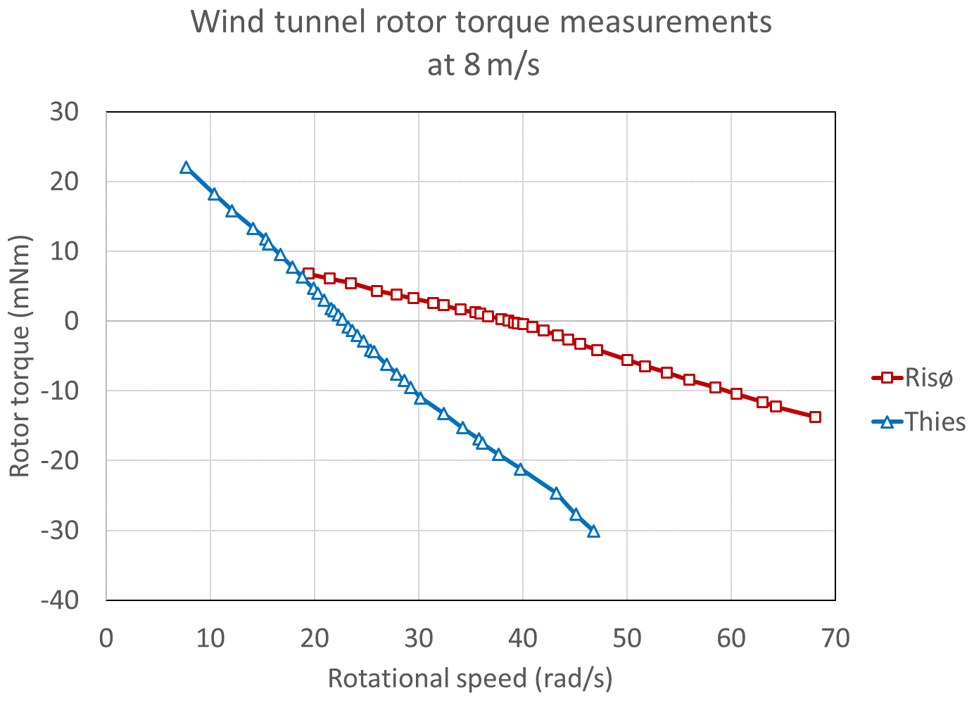
Figure 4Rotor torque measurements of Risø and Thies cup anemometers in a wind tunnel at 8 m s−1 and at varying rotor speed. Data are from Dahlberg et al. (2006).
However, Pedersen (Dahlberg et al., 2006) found the speed ratio definition to be not valid for stationary conditions, i.e. wind tunnel calibration conditions. Calibrations have gain and offset. The bearing friction can explain some of the offset, but some offset remains due to aerodynamic characteristics. This offset was named the “threshold wind speed Ut” and was introduced into the expression of the speed ratio in order to fit torque data to the calibration expression. The nature of the threshold wind speed has not yet been explained:
The normalized rotor torque coefficient curves of the Risø and Thies cup anemometers from the ACCUWIND project are shown in Fig. 5.
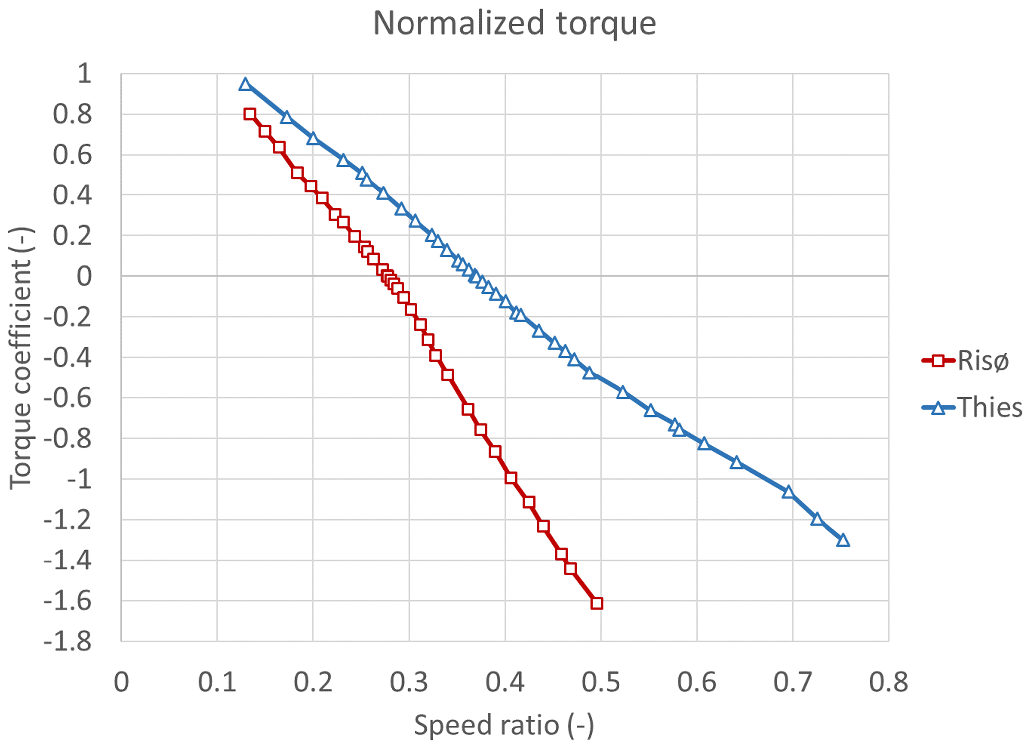
Figure 5Rotor torque coefficient curves of Risø and Thies cup anemometers derived from Fig. 4.
In the CLASSCUP project, Dahlberg (Dahlberg et al., 2001) also verified the influence of plane longitudinal wind variations. Dahlberg generated sinusoidal air flow in the wind tunnel by rotating two vanes in the outlet of the tunnel and found, directly, the overspeeding of the Thies and Risø cup anemometers at an average flow speed of 8 m s−1, as shown in Fig. 6. The amplitude was varied by offsetting the angles between the vanes, and the frequency was varied by the rotational speed of the vanes. The Thies cup anemometer shows significantly higher maximum overspeeding levels than the Risø cup anemometer. The overspeeding of the Risø cup anemometer is slightly negative and close to zero at low turbulence intensity and low frequency.
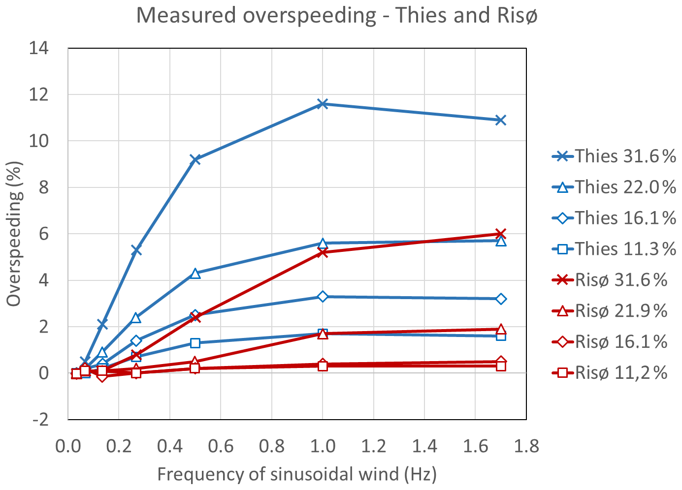
Figure 6Dynamic overspeeding measurements of Thies and Risø cup anemometers in a wind tunnel with sinusoidal wind speed variations. Average tunnel wind speed was 8 m s−1 and with turbulence intensities of 11 %, 16 %, 22 % and 32 % (). Data are from ACCUWIND (Dahlberg et al., 2006).
Dahlberg (Dahlberg et al., 2006) also showed that torque measurements could be extracted from response tests with sinusoidal flow for very small time steps, assuming constant torque over one time step, using the following formula, where I is the cup rotor inertia:
Dahlberg found good correlation between dynamic response tests and static torque measurements. He used dynamic response tests to make torque measurements of cup anemometers also in tilted conditions. The project team found that the overall response in tilted position to a high degree was similar to the response when they first applied the influence of the angular response and afterwards the dynamic response at horizontal flow. The method, by first applying the angular response and then the dynamic response, was then considered robust; the procedure was adopted in the so-called ACCUWIND method.
The overspeeding curves in Fig. 6 clearly show the overspeeding effects, while the torque coefficient curves in Fig. 5 reveal very little about the overspeeding effects. Most obvious from Fig. 6 is the maximum overspeeding level at higher frequencies, where the cup rotor inertia reduces rotational variations and keeps rotational speed practically constant.
The two cup anemometer types represent typical differences in overspeeding characteristics by cup rotors with hemispherical and conical cups, as investigated by Scrase and Sheppard (1944). They introduced general use of conical cups to the Met Office in London, substituting hemispherical cups. The differences in torque characteristics and the advantage of conical cups were not discovered in wind energy before the CLASSCUP and ACCUWIND projects (2001–2006). The IEA document (Hunter et al., 1999) did not mention how these differences in rotor design affected the overspeeding characteristics.
The influence of dynamics by the cup rotor inertia is also evident in step responses, i.e. the response to a sudden change in wind speed. Maximum overspeeding and step responses describe the essence of dynamic overspeeding characteristics. They are, therefore, the focus in the following assessment of cup anemometer models.
In comparison of different models, we use the same nomenclature for all models throughout the text. Models from historical references are only presented in this context if they consider integrated torque over one revolution.
All models start with an introduction of the general equation of dynamics that includes aerodynamic and bearing friction torque:
Here, I is the rotor inertia, ω is the cup rotor speed, QA is the aerodynamic forces and QF the frictional forces. QA includes all aerodynamic forces due to wind from all directions. However, when dynamic effects are studied, the bearing friction torque is often omitted, and only the horizontal unidirectional wind component is considered.
Schrenk (1929) presented a mathematical model of the cup anemometer, i.e. the two-cup drag model (see Fig. 7). On the left side, a high drag coefficient CDH represents the high drag due to the flow into the open cup, while a low drag coefficient CDL represents the low drag due to the flow over the aerodynamically shaped front of the cup. The high drag on the left side will force the cup rotor to rotate clockwise, while the low drag on the right side will reduce the clockwise rotation.
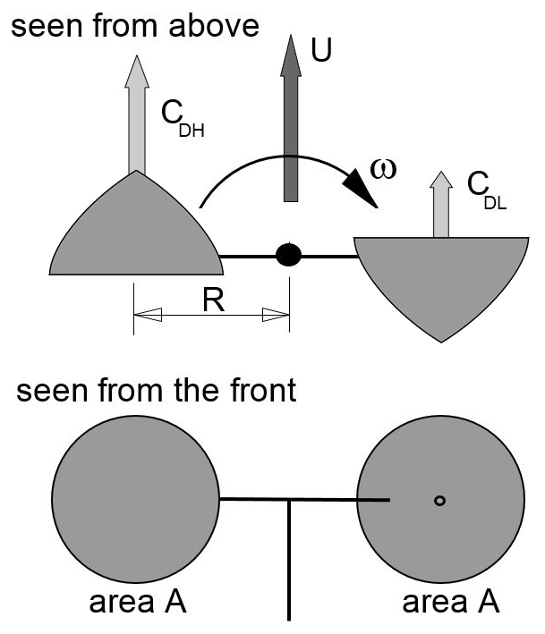
Figure 7The drag model (not the original Schrenk sketch) with two cups on either side of the rotor; one cup on the left side with high drag coefficient CDH and another cup on the right side with low drag coefficient CDL.
The torque balance with the drag model is in this context expressed as
Here DH and DL are the drags corresponding to the two drag coefficients. The drag model is convenient because the low and high drag coefficients are the only constants containing aerodynamic properties to describe torque characteristics.
Since Schrenk (1929), the drag model has been used by several authors, e.g. Wyngaard (1981), Westermann (1996), Hunter et al. (1999), Pedersen and Paulsen (1999), and Pindado et al. (2014) (among others). The drag model was widely considered a valid and simple model to describe the dynamics of cup anemometers.
Schrenk (1929) also presented a parabolic model with more constants. Here we present a fully flexible parabolic model with three convenient constants, also including Schrenk's more general model. The three constants are descriptive and easy to understand. They express the same as many other parabolic models and lead to equivalent results. The torque coefficient is a parabolic function of the speed ratio λ, which has one specific root λ0, i.e. the equilibrium speed ratio, related to the calibration expression. It is then obvious to add the second root of the parabola in formulation of the parabolic torque coefficient model. The model is then expressed as
The first root, , relates to the gain of the calibration line (omitting the threshold wind speed and bearing friction). The second root, λ1, is a constant that basically determines the curvature of the torque coefficient curve in the area around the equilibrium speed ratio, and β is an amplification factor that relates to the slope of the torque coefficient at equilibrium speed ratio:
Second-order perturbation models include Wyngaard et al. (1974), Busch and Kristensen (1976), and Coppin (1982). Rather than considering the time domain, they considered second-order fluctuations or perturbations from equilibrium states. Kristensen (1998) mentions a phenomenological forcing model, based on more physical parameters. In principle, this model is also a parabolic torque model. The drag model, the perturbation models and the phenomenological forcing model all make use of second-order or parabolic torque characteristics. Results obtained with these models will therefore all be similar to results obtained with the parabolic torque coefficient model presented in Eq. (7).
The linear model, with linear torque characteristics even simpler than the parabolic model, is expressed as
The ACCUWIND model makes use of tabulated torque data, measured with a torque sensor in a wind tunnel, like Schrenk (1929), Wyngaard (1981) and others. The normalization process uses the same expression for the torque coefficient (Eq. 1). However, the speed ratio is different from Schrenk's, as Pedersen (Dahlberg et al., 2006) introduced the threshold wind speed Ut in order to fit torque data to the calibration line (see Eq. 2).
In case the bearing friction is zero, the calibration offset Bcal reduces to the threshold wind speed Ut, and the expression for equilibrium speed ratio λ0 is transformed into the linear calibration expression:
When friction is applied, the calibration offset Bcal gets larger than the threshold wind speed Ut, and the slope Acal increases slightly.
The ACCUWIND model is the most general cup anemometer model as it uses tabulated data for tilt response, normalized torque and bearing friction. Normalization of the torque data is made by first extracting the friction torque from measured torque and then normalizing the aerodynamic torque with the target to fit Ut to the calibration constants Acal and Bcal at the calibration conditions. Fitting is made by simulation of the wind tunnel calibration, including the use of realistic turbulence intensity, e.g. 1 % isotropic von Karman turbulence. A small speed ratio correction factor λcorr might be necessary to apply because torque measurements and calibration measurements may be made at different air temperatures and air densities in the wind tunnel, and these differences are enough to disturb a correct fitting. Simulation with the ACCUWIND model is made with a 10 min time-based 3D wind file, generated with the Mann (1994, 1998) model. At each time step, the instantaneous wind vector and upflow angle are determined. With the rotational speed and the upflow angle, the angular response is interpolated in the tabulated angular response data. The angular response is multiplied to the scalar of the wind vector to derive the resulting equivalent horizontal wind speed Ueq. The torque coefficient CQA(λ) is then derived by interpolation in the normalized torque coefficient table with the Ut-adjusted speed ratio.
The friction torque QF is found by interpolation in the friction table with the rotor speed ω and the air temperature T. Change in angular speed is found with the incremental time step Δt:
The actual response of a 10 min wind speed input with N time steps is determined by going through successive time steps to determine the “measured” wind speed . The “true” average of the horizontal input wind speed is . The systematic deviation is determined by the true minus the measured.
Overspeeding characteristics of cup anemometers is best illustrated (as shown in Fig. 6) by the response to sinusoidal longitudinal horizontal wind variation and with step responses. The drag model, the parabolic model, the linear model, the partial linear model and the ACCUWIND model are now assessed and compared for maximum overspeeding characteristics and step responses.
5.1 Overspeeding with the ACCUWIND model
The overspeeding of the Risø and Thies cup anemometers, calculated with the ACCUWIND model, is shown in Figs. 8 and 9. The calculations show good agreement with the wind tunnel measurements, both with respect to the maximum overspeeding levels as well as the increase of overspeeding with frequency.
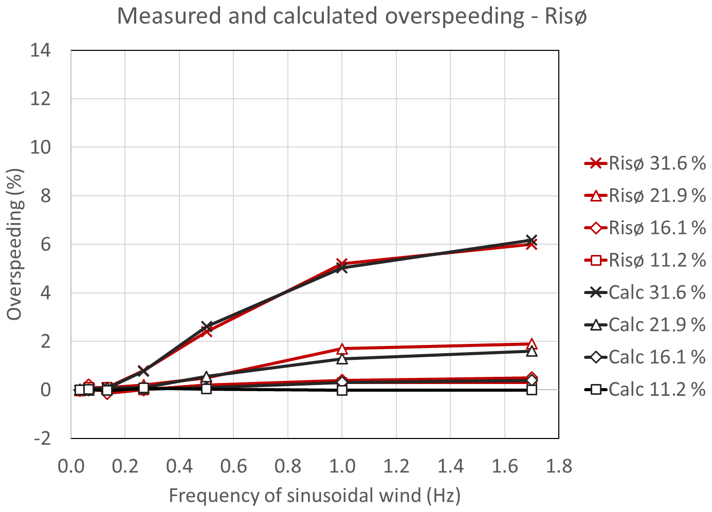
Figure 8Dynamic overspeeding measurements and ACCUWIND calculations of the Risø cup anemometer with sinusoidal wind speed variations. Average tunnel wind speed was 8 m s−1 and with different turbulence intensities (). Torque data are from Fig. 5.
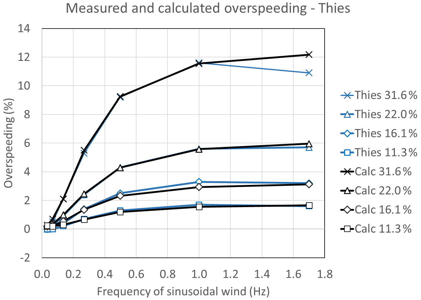
Figure 9Dynamic overspeeding measurements and ACCUWIND calculations of the Thies cup anemometer with sinusoidal wind speed variations. Average tunnel wind speed was 8 m s−1 and with different turbulence intensities . Torque data are from Fig. 5.
5.2 Maximum overspeeding with the parabolic torque coefficient model
The parabolic torque coefficient model is assessed for a typical equilibrium speed ratio λ0=0.3 and for various values of λ1 (see Fig. 10). The slope of the torque coefficient curves at the equilibrium speed ratio is set to , which corresponds almost to the slope of the Risø torque coefficient curve in Fig. 5.
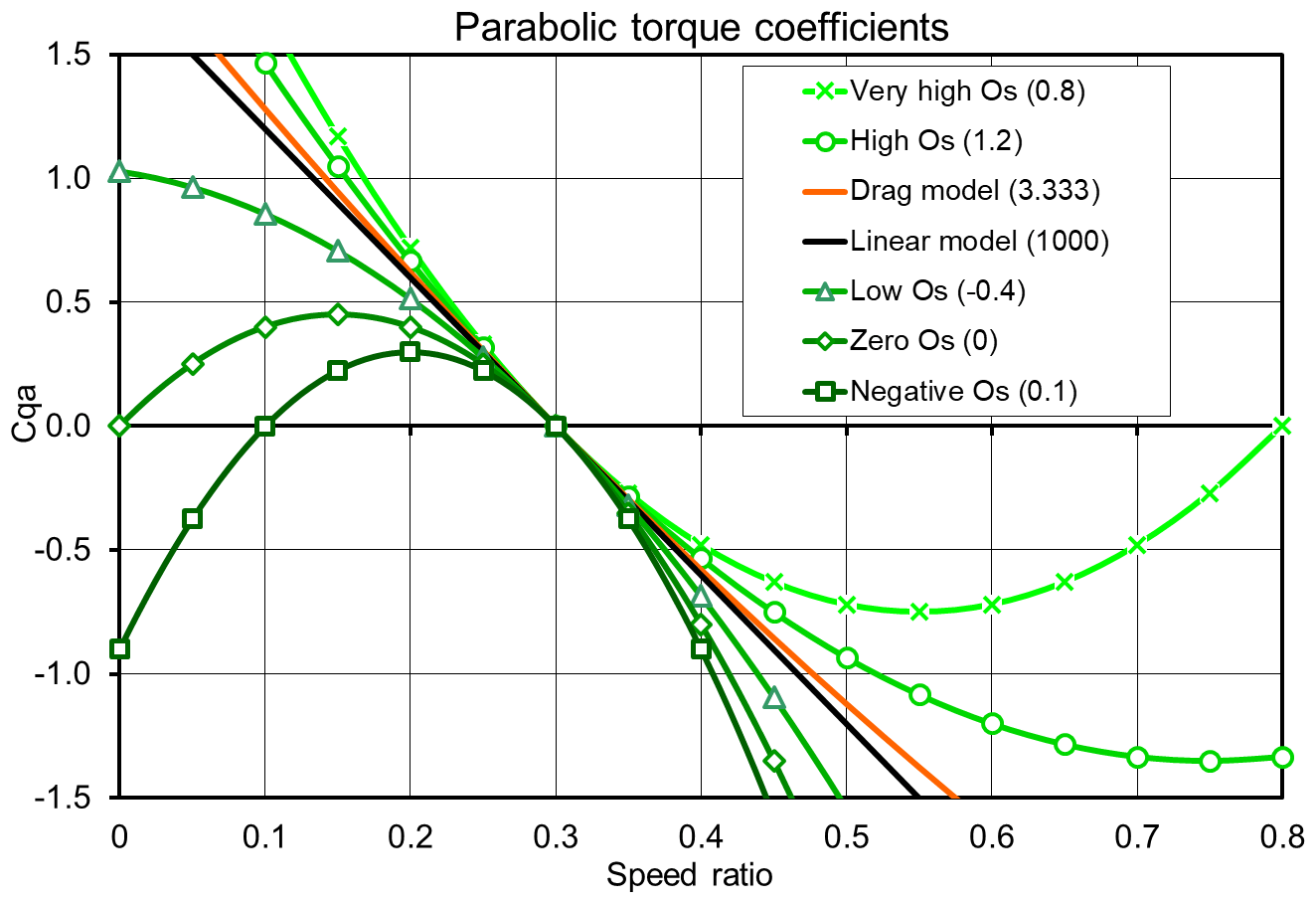
Figure 10Torque coefficient curves for parabolic model with equilibrium speed ratio λ0=0.3 and slope at equilibrium speed ratio . Various values of λ1 as shown in the legend. The linear model is in black, and the drag model is in orange.
An expression of the maximum overspeeding level at high wind speed frequencies is derived from the parabolic torque coefficient expression (Eq. 7). Consider the cup anemometer being exposed to a sinusoidal wind speed U0+ΔUsin (2πft) at a sufficiently high frequency f where the cup rotor angular speed ω0 is constant due to the inertia of the cup rotor. The instantaneous aerodynamic rotor torque is then
Now, integrating the torque over one cycle from t=0 to with the constant cup rotational speed ω0, we have
which integrates to
Setting the integrated torque equal to zero, we find the equilibrium angular speed ω0:
We see that by setting the amplitude of the pulsating variations equal to zero, ΔU=0, we get two roots:
In the case λ1>λ0, the minus sign before the square root gives the first root, which is the equilibrium speed. In the case λ1<λ0, the plus sign gives the first root.
The overspeeding is expressed as the angular speed increase in the pulsating wind divided by the angular speed in the constant wind:
which simplifies to
The standard deviation of a sinusoidal wave is the amplitude divided by the square root of 2, so we have , where Ti is the turbulence intensity. The maximum overspeeding with a parabolic torque coefficient curve is then
The plus sign before the square root is used when λ1<λ0 and minus is used when λ1>λ0. Figure 11 shows the maximum overspeeding of sinusoidal wind as a function of turbulence intensity for the corresponding torque coefficient curves in Fig. 10. The included maximum overspeeding values of the Thies are seen to be a little higher than the drag model and are close to following the same pattern. The maximum overspeeding of the Risø, however, does not seem to follow either of the curves, and the parabolic torque coefficient model seems to fail completely in this case.
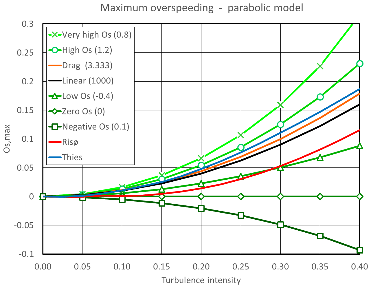
Figure 11Maximum overspeeding of the parabolic torque coefficient model for an equilibrium speed ratio λ0=0.3 and various values of λ1 as shown in the legend and as a function of turbulence intensity. Maximum overspeeding of Risø (red) and Thies (blue) are added.
The expression in Eq. (19) is seen to depend only on the ratio of the roots and the turbulence intensity squared. From the expression, it is observed that the maximum overspeeding is zero when the second root, λ1, is equal to zero. Theoretically, this means that dynamic overspeeding is fully eliminated when the torque coefficient curve is parabolic and the second root is zero. The zero overspeeding is in this case independent of rotor inertia, distance constant and frequency variations.
Kristensen (2002) made an analysis of overspeeding based on the “suspicion”, discovered in the CLASSCUP project, that cup anemometers might have zero or even negative overspeeding. He concluded that dynamic overspeeding is always positive, while it can have negative overspeeding due to non-linear calibration curves and angular characteristics below ideal characteristics. The theoretical analysis shows, however, that dynamic overspeeding can actually be zero for parabolic torque coefficients. Zero and even slightly negative overspeeding values are confirmed with the wind tunnel measurements on the Risø cup anemometer at low turbulence intensities up to 16 %, while the overspeeding at higher turbulence intensities is increasingly positive (Dahlberg et al., 2001, 2006).
5.3 Maximum overspeeding with the drag model
An interesting case, also shown in Figs. 10 and 11, is the case of the drag model. Introducing the torque coefficient into the drag model, Eq. (6), and rearranging, we get
Setting the drag ratio , we find the roots of the polynomial:
We see that the drag model always has a second root reciprocal to the equilibrium speed ratio.
The drag model is a special case of the parabolic torque coefficient model. The maximum overspeeding with the drag model is only dependent on the equilibrium speed ratio and thus dependent on the slope of the calibration line:
As the equilibrium speed ratio is dependent on the ratio between the drag coefficients, the maximum overspeeding is again dependent on the drag coefficient ratio:
The maximum overspeeding for the drag coefficient model is always positive and a little higher than the turbulence intensity squared. For a typical equilibrium speed ratio λ0=0.3, the overspeeding is , which for 10 % turbulence intensity is 1.1 % and for 20 % turbulence intensity is 4.4 %. The drag model thus has a very specific torque coefficient curve and a very specific maximum overspeeding. The maximum overspeeding of the Thies cup anemometer in Fig. 11 is 1.8 % to 5.8 % for turbulence intensities from 11 % to 22 %. These maximum overspeeding values correspond to factors 1.5 to 1.2, which are somewhat larger than 1.10. The Thies cup anemometer is thus more prone to overspeeding than the drag model shows. Opposite with the Risø cup anemometer, where the maximum overspeeding is 0.2 % to 1.8 % for turbulence intensities from 11 % to 22 %, these maximum overspeeding values correspond to factors of 0.2 to 0.4, which are much lower than 1.10. The drag model is thus significantly overestimating the Risø cup anemometer overspeeding, while it underestimates the Thies cup anemometer. The cup shapes shown in Fig. 7 of the two-cup drag model are therefore not shown as conical cups nor hemispherical cups, but something in between. Anyway, the drag model is representative for very limited types of cup anemometers and is not representative for modern conical cup anemometers being used in wind energy today. The parabolic torque coefficient model performs better, because we can fit the data to each maximum overspeeding level at different turbulence intensities.
5.4 Maximum overspeeding with the linear torque coefficient model
Another interesting case, also seen in Figs. 10 and 11, is the linear torque coefficient model with the following torque expression:
In this case, the slope at equilibrium speed ratio κ is equal to the amplification factor β. With a sinusoidal wind and integrating over one cycle, the torque is
and resulting in the following integral:
Setting the torque equal to zero, we find the equilibrium speed:
And the maximum overspeeding of a linear torque is
A linear torque coefficient may also be achieved from the parabolic torque coefficient model when λ1 is going towards ∞ or −∞. In both cases, we find that the maximum overspeeding for a linear torque coefficient is directly proportional to the turbulence intensity squared, i.e. . This is illustrated in Fig. 10 with the curve for λ1=1000. This is about 10 % less than the maximum overspeeding of the drag model. The linear torque model is thus not able to model the torque characteristics of the Thies and Risø cup anemometers to a satisfactory level for the same reasons as for the drag model.
5.5 Maximum overspeeding with the partial linear torque coefficient model
Of more interest is the partial linear torque coefficient model with two linear torque coefficient curves, one at either side of the equilibrium speed ratio. The partial linear torque coefficient model is useful if a cup anemometer torque coefficient curve with an approximation can be considered partial linear in a broad range around the equilibrium speed ratio. The partial linear torque coefficient model was investigated by Pedersen (2011). He found that with the torque in this model he could achieve almost the same results in the classification of five types of cup anemometers as with tabulated data in the ACCUWIND model.
The partial linear torque coefficient curves may be expressed as
For the partial linear torque coefficient model, the maximum overspeeding level can be determined by applying a sinusoidal wind speed as for the linear torque coefficient model. Consider again the cup anemometer to be exposed to a sinusoidal wind speed U0+ΔUsin (2πft) at a sufficiently high frequency f where the rotor angular speed can be assumed constant at ω0.
Now, integrating again the torque over one cycle from t=0 to with constant speed ratio ω0, we add the torque on each side:
The approximation sign is due to the fact that the torque on either side is not exactly half of each cycle, but this is an error that is very small and omitted here. Using the results from the linear torque coefficient model and setting the integrated torque equal to zero we find the equilibrium angular speed ω0:
The maximum overspeeding is thus
As , the expression is converted to
When κlow=κhigh, we get as for the full linear torque coefficient curve. Partial linear torque coefficient curves are shown in Fig. 12 for various ratios. The maximum overspeeding of cup anemometers with partial linear torque coefficient is shown in Fig. 13. The maximum overspeeding of the Thies is seen almost to follow the ratio 1.2 curve, and the shape is quite similar. The maximum overspeeding of the Risø seem to follow close to the ratio 0.8 curve. This indicates that the partial linear model seems to be a better fit to the two cup anemometers than the parabolic torque coefficient model. It confirms the experience that the partial linear model performs quite well in classification of the cup anemometers (Pedersen, 2011).
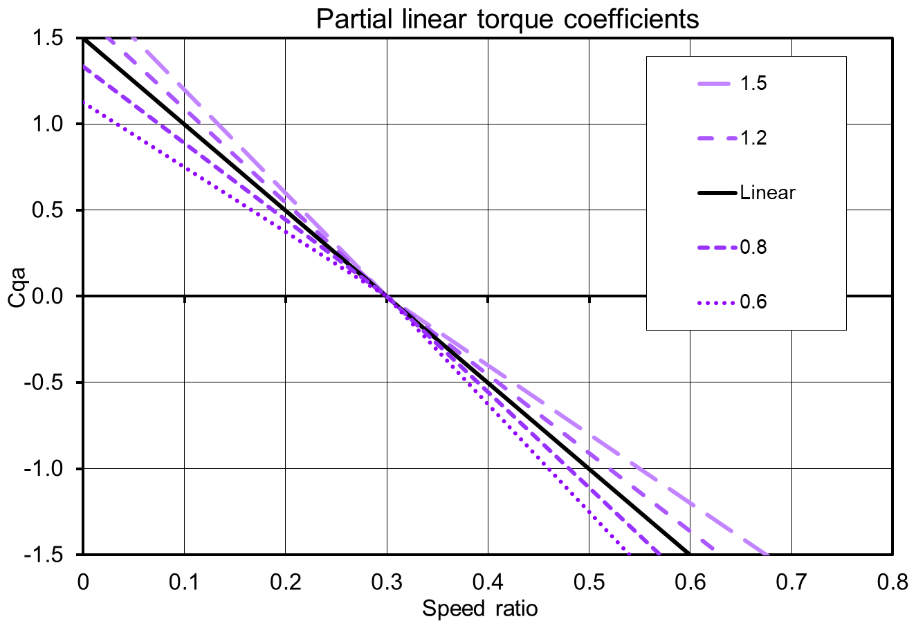
Figure 12Torque coefficient curves for partial linear model with various κ ratios. Linear model in black.
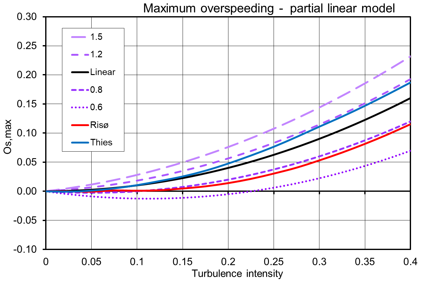
Figure 13Maximum overspeeding of partial linear torque coefficient model for various κ ratios.
We cannot achieve maximum overspeeding equal to zero for all turbulence intensities as for the parabolic torque coefficient model when λ1=0. We have zero maximum overspeeding for the following κ ratios:
For turbulence intensities 5 %, 10 %, and 15 %, the optimum κ ratios are, for example, 0.89, 0.80, and 0.71, respectively.
6.1 Step response with the parabolic torque coefficient model
The differential equation for the parabolic torque coefficient model (Eq. 7) is rearranged to an expression in ω (setting friction and threshold wind speed to zero):
We now make the following substitution:
which, expressed in rotor rotational speed, is
with the following derivative:
Inserting expressions of the substitution and rearranging, Eq. (36) becomes
Defining now the distance constant l0 and inserting the slope of the torque coefficient curve at the equilibrium speed ratio λ0, we can express the distance constant as
This distance constant is a general constant for a cup anemometer with a parabolic torque coefficient curve throughout the parabolic speed ratio range. Observe that the slope of the torque coefficient curve κ, at equilibrium speed ratio λ0, is always negative, which makes the distance constant positive. Inserting and rearranging, the substituted differential equation is expressed in a simple and general form:
This equation is a first-order linear ordinary differential equation. It can be solved analytically for different input wind speeds as a function of time t. The general solution in s is
Here C is a constant that must satisfy the starting requirements at t=0. Inserting s and rearranging, we get the general analytical solution for the cup rotor angular speed for the parabolic torque coefficient model:
If the cup anemometer is given a step input ΔU from U0 to Us, we find . Integrating and rearranging, we get the general solution to the step response of a cup anemometer with parabolic torque coefficient:
For t going towards infinity, the equation goes towards the static solution . For λ1=0, the case with zero maximum overspeeding, we get the following simpler equation:
Figure 14 shows upwards step responses from 6.7 to 10 m s−1 for the different torque coefficient curves in Fig. 10. Figure 15 shows downwards step responses from 13.3 to 10 m s−1 for the same torque coefficient curves. The corresponding speed ratio ranges are from 0.2 to 0.3 and from 0.4 to 0.3, so we are within the speed ratio ranges where the torque coefficient curves have negative slopes. The step responses deviate significantly. The torque coefficient curve with negative maximum overspeeding is the slowest in stepping up, while it is the fastest in stepping down. The opposite is the case for the higher maximum overspeeding torque coefficients. Figure 16 shows the differences in stepping up to stepping down from Figs. 14 and 15. The very high and high overspeeding cases and the drag model case are speeding up faster than they slow down. The linear torque coefficient model have no difference between stepping up and stepping down, i.e. it slows down just as fast as it speeds up, but still it has a positive overspeeding with the turbulence intensity squared. The zero overspeeding case slows down faster than it speeds up. This is a bit different than the commonly explained understanding that overspeeding is due to speeding up faster than slowing down (Busch and Kristensen, 1976; Wyngaard, 1981; Hunter et al., 1999). However, the simple explanation of the overspeeding concept is valid for varying wind (e.g. sinusoidal wind) and not for a constant wind, as in this case of step responses. Even though slowing down is equal to speeding up in step responses, there will still be an overspeeding in a varying wind, because the aerodynamic forces on the cup rotor are dependent on the wind speed squared. The torque coefficient curve has to counteract on this squared dependency to eliminate overspeeding, and the linear torque coefficient is not enough to do this. Only the parabolic torque coefficient curve with the second root through zero can meet this requirement.
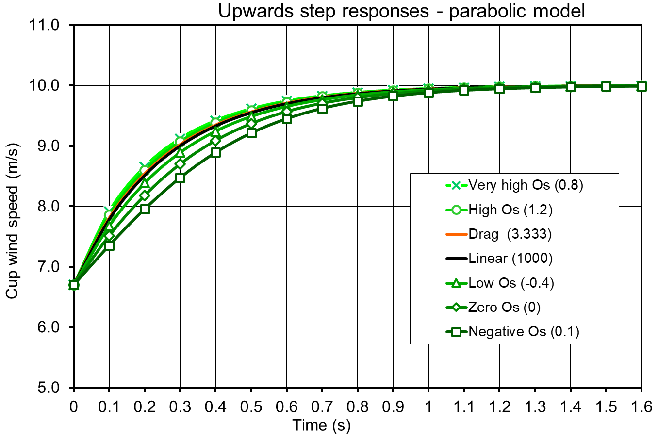
Figure 14Step up response from 6.7 to 10 m s−1 for cup anemometers with parabolic torque coefficient curves.
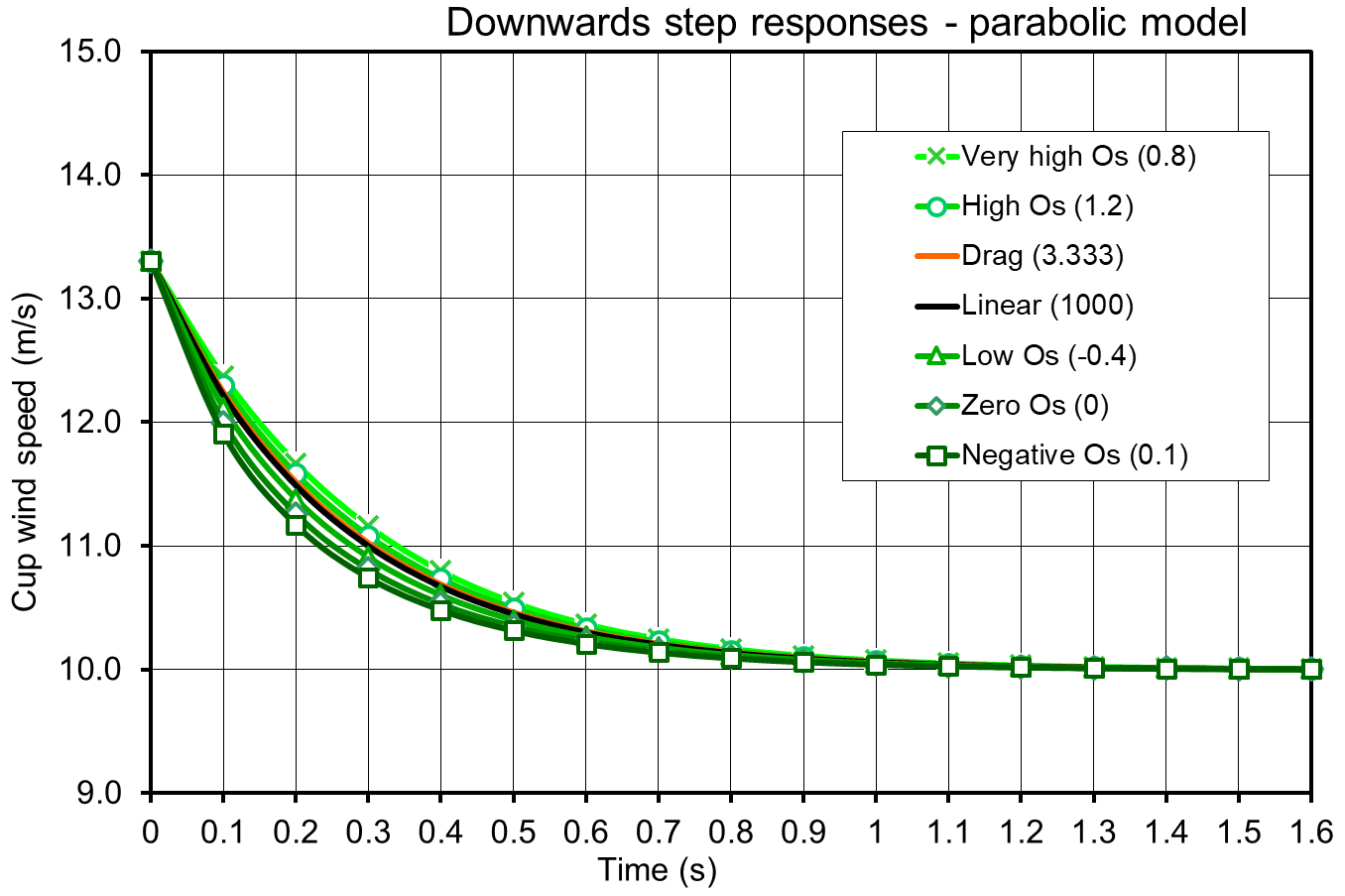
Figure 15Step-down response from 13.3 to 10 m s−1 for cup anemometers with parabolic torque coefficient curve.
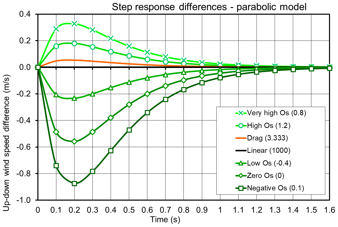
Figure 16Step response differences between stepping up to 10 m s−1 and stepping down to 10 m s−1 for cup anemometers with parabolic torque coefficient curves.
6.2 Step response with the linear torque coefficient model
The linear torque coefficient model is expressed by
This expression can be interpreted as a special case of the parabolic torque coefficient model with λ1→∞ or , as shown before, and where the slope κ is equal to the amplification factor β.
Linear model dynamics can by insertion of the distance constant l0 be expressed by
This is a first-order linear ordinary differential equation with the following solution:
With a step response from a wind speed U0 and angular speed ω0 at time t=0 to a tunnel wind speed , we find C=ω0 and
This is the same expression we achieve for λ1→∞ or in Eq. (45) for the parabolic model. Inserting the time constant , we get
Equation (51) is equal to the step response formula in the Hunter et al. (1999) recommendation for a step response from a certain rotor angular speed (over or under equilibrium speed ratio). Setting ΔU=Us for a step response from standstill, we get
Equation (52) is equivalent to the step response equations from stand still described in the ISO standard (ISO, 2007) and the ASTM standard (ASTM, 2017). The IEA, ISO and ASTM documents describe methods to measure the distance constant with step responses. They define the distance constant as the distance the air flows past a rotating anemometer during the time it takes the cup wheel to reach or 63.2 % of the equilibrium speed after a step change in wind speed. If we insert t=τ in Eq. (52), we find exactly this value. The IEA, ISO and ASTM documents, with their formulas, all relate to linear torque coefficient curves. Measuring the time to reach 63.2 % of equilibrium speed corresponds to use torque coefficient data for speed ratios from zero to 0.632×λ0.
The IEA recommendation (Hunter et al., 1999) included a linear regression method for determination of the time constant τ in a step response. The time constant should be derived from Eq. (51) with a method to fit the data to the formula:
Here , where l0 is the distance constant and U0 is the constant wind speed during the step response. The method uses a linearization with the natural logarithm:
Pedersen (2011) used the IEA method but found the speed ratio ranges in the analysis (0 %–63.2 %) being far from the range that is most relevant. For the upwards step response, he found the appropriate equilibrium speed ratio range to be 50 %–98 %, and for the downwards step response it was 150 %–102 %. These speed ratio ranges would better represent the torque for the relevant turbulence intensities. The ISO method recommends 30 %–74 %, but this range is also far from the relevant speed ratio range.
With a linear regression of the measured data in Eq. (54), the slope of the step response may be determined, and from the slope τ is derived. With the distance constant relation l0=τU0, the slope of the torque coefficient at λ0 is found from Eq. (41):
6.3 Step responses with the partial linear torque coefficient model
The partial linear torque coefficient model is of more interest than the linear model because torque coefficient curves of actual cup anemometers fit better to this model. For this model, step responses can be used to determine the torque characteristics, as shown in the former section. In this case, we just have two different slopes to determine with step responses made from either side of the equilibrium speed ratio. The early step response measurements by Barton (1989) actually found two different distance constants for each cup anemometer type, and these could have been used to determine partial linear torque coefficients. Step responses can be utilized in practice to determine the slopes κlow and κhigh, to fit to a partial linear torque model (Pedersen, 2011). Methods to do this were adopted as an approximate method in the IEC standard (IEC-12-1, 2017) as an alternative method, in case detailed and tabulated torque measurements are not available for classification.
In deriving the step response characteristics, the distance constant of a cup anemometer with a parabolic torque coefficient curve was defined as
This constant is a general constant within a parabolic torque coefficient speed ratio range, including the drag and linear models. We also found that the distance constant for step responses of cup anemometers in several standards and references is determined from the step wind speed and the time constant:
The deduction of a step response expression from a cup anemometer with a parabolic torque coefficient curve showed that these two expressions are coincident. The common assumptions and procedures must therefore be that torque coefficient curves are parabolic. This is, however, an assumption far from correct, confirmed from Figs. 5 and 6. And this is why distance constants derived with procedures from the standards ASTM (2017) and ISO (2007) may give quite different results, specifically between step responses from low- and high-speed ratios but also between different wind speed step responses. From Eq. (56), it is seen that the distance constant is expressed directly as a function of the torque coefficient slope κ at the equilibrium speed ratio λ0. It makes much more sense to relate the distance constant to the tangent of the torque coefficient at equilibrium speed ratio rather than to relate it to the time it takes the cup wheel to reach 63.2 % of the equilibrium speed after a step change, as it is defined in the ASTM and ISO standards. Distance constants should be extracted from step response data as close to equilibrium speed ratio as possible, as it is described in the procedure of IEC (IEC-12-1, 2017) in order to make them relevant to wind speed measurements.
When Barton (1989) found different distance constants for a cup anemometer, it was a clear indication that torque curves did not follow parabolas. Barton found two distance constants of a cup anemometer, consistent with the theory of partial linear torque coefficient curves. The partial linear torque coefficient model is in many cases a better mathematical model than the parabolic torque model in fitting torque data of modern cup anemometers with conical cups. But in fact, the distance constant is not an inherent constant of a cup anemometer, because the torque coefficient curve varies a lot more than a parabolic curve. For a detailed analysis, and specifically for an IEC classification, it is important to use the wind-tunnel-measured and tabulated torque coefficient curve.
Dahlberg (Dahlberg et al., 2001, p. 44) made a significant number of dynamic tests on cup anemometer configurations. He found that the overspeeding effect was primarily dependent on the cup rotor design, as shown with the Thies and Risø cup anemometers (Fig. 6). It was a revelation that hemispherical cup rotors provide significantly more overspeeding than conical cups, which is the same as Scrase and Sheppard verified in 1944. Dahlberg found, however, that a fat cup anemometer body could spoil low overspeeding of a cup rotor with conical cups. The findings indicate that cup anemometer overspeeding is dependent on the whole design of the instrument. Good designs can almost eliminate the overspeeding effect, while other designs trigger significant overspeeding.
For the cup anemometer rotor itself, the maximum overspeeding can be zero when the second root of a parabolic torque coefficient curve is zero. An optimized cup anemometer rotor has to have good starting torque characteristics, and this does not imply zero torque at the second root. An optimized cup anemometer rotor should have an optimized parabolic torque coefficient curve limited to an appropriate range around the equilibrium speed ratio λ0, and with perhaps linear tangential curves outside of this range. An optimized cup anemometer rotor with this type of torque coefficient curve would achieve zero overspeeding for low and medium turbulence intensities and increasing overspeeding for high turbulence intensities. The requirement of low inertia of the cup rotor is well-known from research by meteorologists, but having part of the torque coefficient curve with zero overspeeding is new.
Description of an optimized torque coefficient curve could start from rotor stand still. Schrenk (1929) estimated starting torque from the drag model. He used the drag coefficients of hemispherical cups at straight angles to the wind (CDH=1.33 and CDL=0.33) to get the starting torque coefficient . Hoerner (1965) found a little higher values: CDH=1.42 and CDL=0.38. Brevort and Joyner (1934) found CDH=1.40 and CDL=0.40 for a hemispherical cup and CDH=1.40 and CDL=0.48 for a conical cup. The Risø and Thies cup anemometers in Fig. 5 seem to reach CQA0=1.0 at speed ratios about λ=0.1. where the curves are still going up. Torque coefficient measurements by Dahlberg (2001) support the limitation to CQA0=1.0. Extrapolation of the Risø and Thies torque coefficient curves, however, reach 1.5 at λ=0 for both, and we therefore set this point as a basis for extrapolation of the linear curves.
With these start-up conditions and with a determined equilibrium speed ratio λ0=0.3 we let the linear torque coefficient curve converge to the tangent of a zero overspeeding parabolic torque coefficient curve. The amplification factor β of the zero overspeeding parabolic torque coefficient curve is in this case
Here λ2 is the speed ratio of the merging linear and parabolic model curves below λ0.
The speed ratio variations of a cup anemometer are not symmetric around equilibrium speed ratio λ0 in a natural varying wind. For the maximum overspeeding cases with sinusoidal wind, the speed ratio variations extend 1.4, 2.0 and 3.1 times higher compared to low-speed-ratio values for turbulence intensities of 12 %, 24 % and 36 %, respectively. High speed ratios are reached when wind speed falls to lower values. In the limiting case at very high speed ratios, the cup rotor runs in relatively calm wind, and only the low drag of the cups produces torque. In this very high speed ratio case, the cup drag might be considered proportional to the cup speed squared times 3 for the three cups. The optimum zero overspeeding speed ratio range is, in the optimized case however, considered symmetric around the equilibrium speed ratio, although this is not optimum but perhaps more realistic. For higher speed ratios, we assume a linear curve, tangent to the parabolic curve, until reaching the limiting very high speed ratio case.
With this description of an optimized torque coefficient curve; with the values CQA0=1.0, CQA0lin=1.5, λ0=0.3, and λ1=0; and with intersection points between linear and parabolic curves λ2=0.28, 0.26, and 0.24, respectively, three optimized torque coefficient curves are shown in Fig. 17. The three λ2 values correspond to 7 %, 14 % and 20 % of equilibrium speed ratio, respectively. The slope ratio for the linear parts corresponding to the three λ2 values are 0.76, 0.58 and 0.43, respectively. The Risø and Thies torque coefficients are shown in Fig. 17, as well. The Thies curve is seen to curve upwards while the other curves are curving downwards. This indicates the tendency that torque coefficient curves need to have for more optimum overspeeding characteristics.
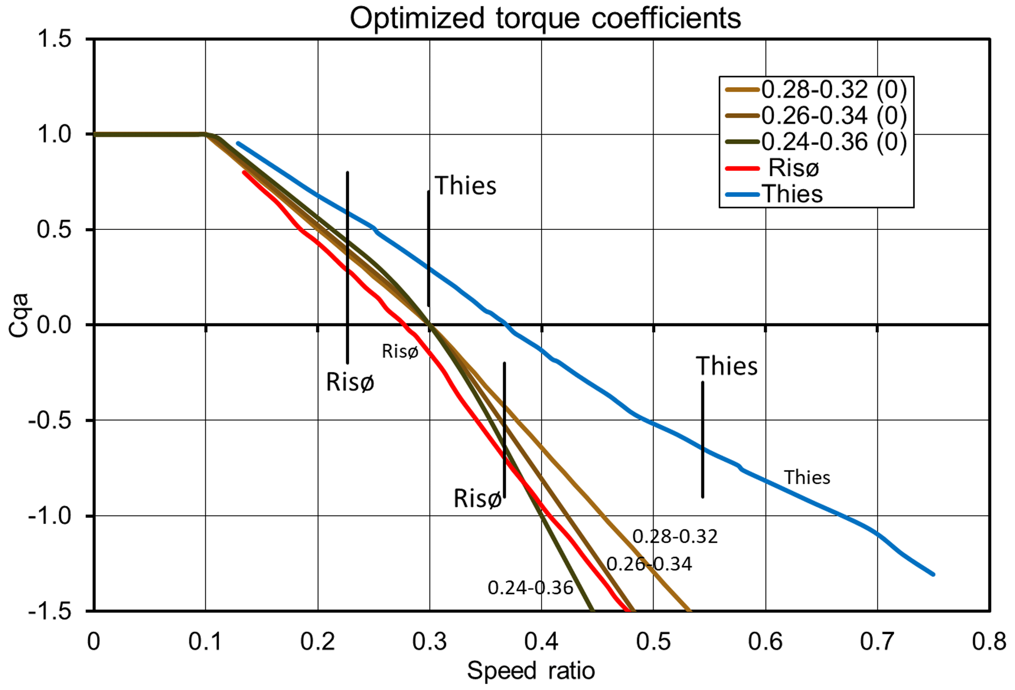
Figure 17Optimized torque coefficient curves for CQA0=1.5, λ0=0.3, λ1=0.0, and parabolic ranges, 0.28–0.32 (light beige), 0.26–0.34 (medium beige), and 0.24–0.36 (dark beige). Added Risø (red), Thies (blue); data are from Fig. 6. Vertical black lines are minimum and maximum speed ratio markings for 8 m s−1 and 20 % spectrum turbulence intensity.
The maximum overspeeding curves for torque alone, and otherwise with Risø cup anemometer dimensions and rotor inertia, except for Thies, are calculated with the ACCUWIND code and are shown in Fig. 18. Also included are maximum overspeeding curves for Risø and Thies. Risø and Thies are actual cup anemometers with individual dimensions and rotor inertia, but the Risø cup anemometer is the one that is interesting to optimize incrementally, and this is why the Risø properties are used.
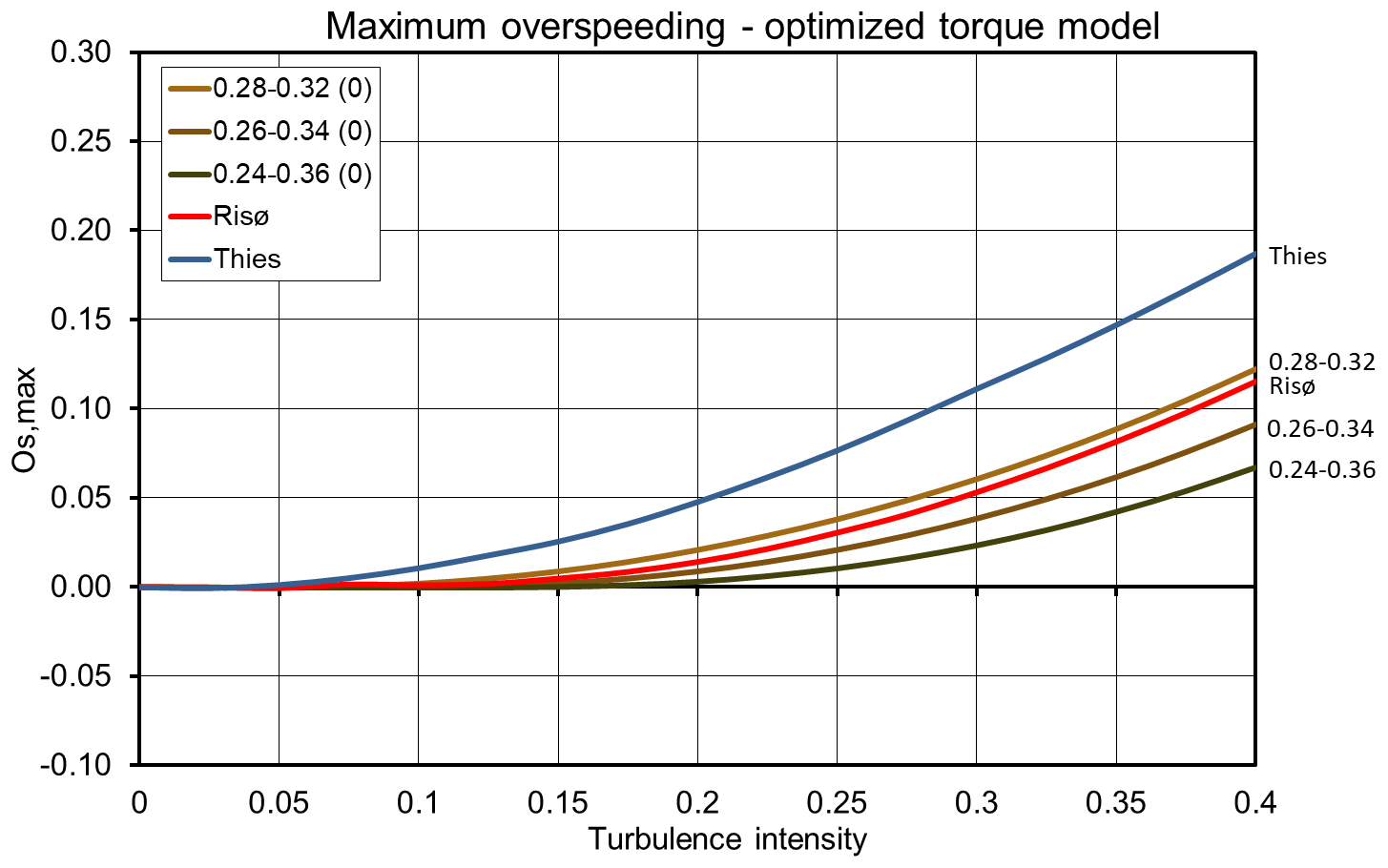
Figure 18Maximum overspeeding at sinusoidal wind of 8 m s−1 average wind speed for optimized torque coefficient curves from Fig. 17, calculated with same dimensions and inertia as Risø. Added Risø (red) and Thies (blue, and with Thies properties).
The Thies cup anemometer seems to deviate from the optimized torque curves with significantly higher maximum overspeeding. The Risø cup anemometer seems to fit to the optimized torque curve shapes. A best fit might be to a 0.27–0.33 optimized torque curve.
The proposed optimum torque coefficient curves with zero overspeeding in certain speed ratio ranges have very low maximum overspeeding up to medium high turbulence intensity. For the Risø cup anemometer, the low maximum overspeeding is up to about 12 % turbulence intensity. The Thies cup anemometer seems to do good up to about 5 % turbulence intensity.
Low overspeeding in field measurements requires low maximum overspeeding level as well as low inertia of the cup anemometer rotor. The maximum overspeeding level is independent of rotor inertia, but low rotor inertia can keep the cup anemometer from operating for too long at the maximum overspeeding level.
The overspeeding in actual wind with a wind spectrum is calculated with the ACCUWIND model, using Mann (1998) turbulence code with a Kaimal spectrum and length scale Lu=350 m. Only torque is considered (i.e. no friction), tilt response is cosine-shaped and threshold wind speed is set equal to zero. All calculations are with Risø dimensions and rotor inertia, except for Thies (see Fig. 19).
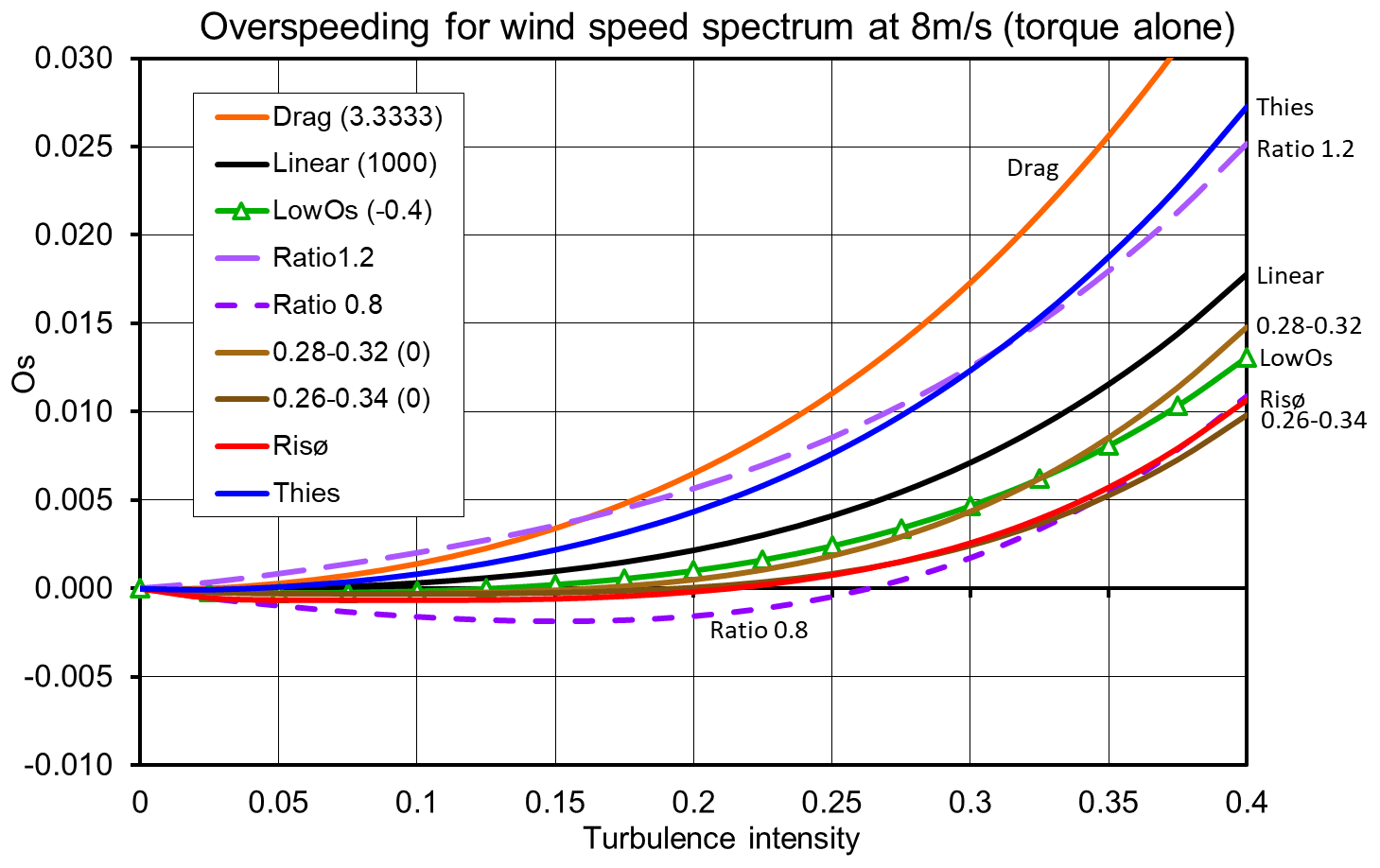
Figure 19Overspeeding for Kaimal wind spectrum () at 8 m s−1 average wind speed. Curves include three parabolic model curves (drag (orange), linear (black), and low Os (green)), two partial model curves (ratio 1.2 (long-dashed purple line) and ratio 0.8 (short-dashed purple line)), two optimized torque model curves (0.28–0.32 (light beige) and 0.26–0.34 (medium beige)), and finally Risø (red) and Thies (blue). All calculations are with Risø dimensions and inertia, except for Thies.
The overspeeding wind spectra show significantly reduced overspeeding from the maximum overspeeding curves. Note that the overspeeding scale is reduced by a factor 10. The Thies overspeeding is about one-tenth of the maximum overspeeding and is about half that between the linear and drag models, which are based on the Risø inertia. The Risø overspeeding is zero or slightly negative up to 20 % turbulence and is reduced from 20 % to 35 % turbulence by about a factor of 20. Risø is very close to the 0.26–0.34 speed ratio case.
Calculations of the IEC Classes A and B, where whole ranges of wind speed and turbulence spectra are included, are shown in Table 1 for the torque characteristics alone. The two last rows also include angular response and friction data of Risø and Thies. The Thies Classes 0.46A and 1.28B lie well between the linear and drag models, and Risø with Classes 0.08A and 0.54B lies between the 0.28–0.32 and 0.26–0.34 optimum torque cases. The overspeeding values are in general not more than half a percent for Class A and only the drag ratio of 1.2 and Thies cases come above 1 % in Class B. The classification changes significantly when the angular characteristics from Fig. 3 and friction are included, and Thies classes change to 1.55A and 7.23B and Risø classes change to 1.26A and 5.25B. The torque characteristics only contribute with 30 % for Class A and 18 % for Class B for Thies, and 6 % for Class A and 10 % for Class B for Risø. Torque characteristics are not the main cause of systematic deviations. Angular characteristics take the lead here, but torque characteristics are still an important characteristic to take into account, especially when higher frequency content of wind spectra occur.
Table 1IEC classification with the ACCUWIND model for torque alone (no friction, cosine tilt response, zero threshold wind speed), except for last two rows for Risø and Thies, where all influence parameters are included. Torque curves from Figs. 5, 10, 12 and 17. All calculations with Risø dimensions and inertia, except for Thies.
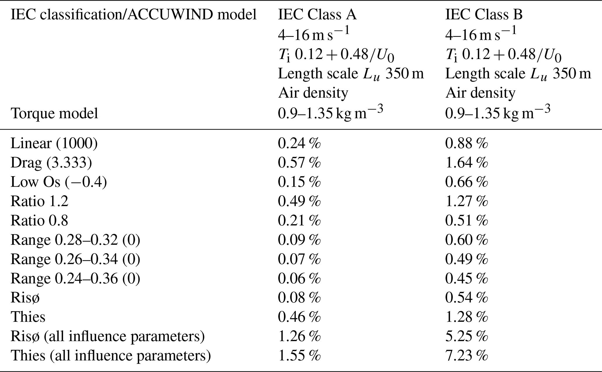
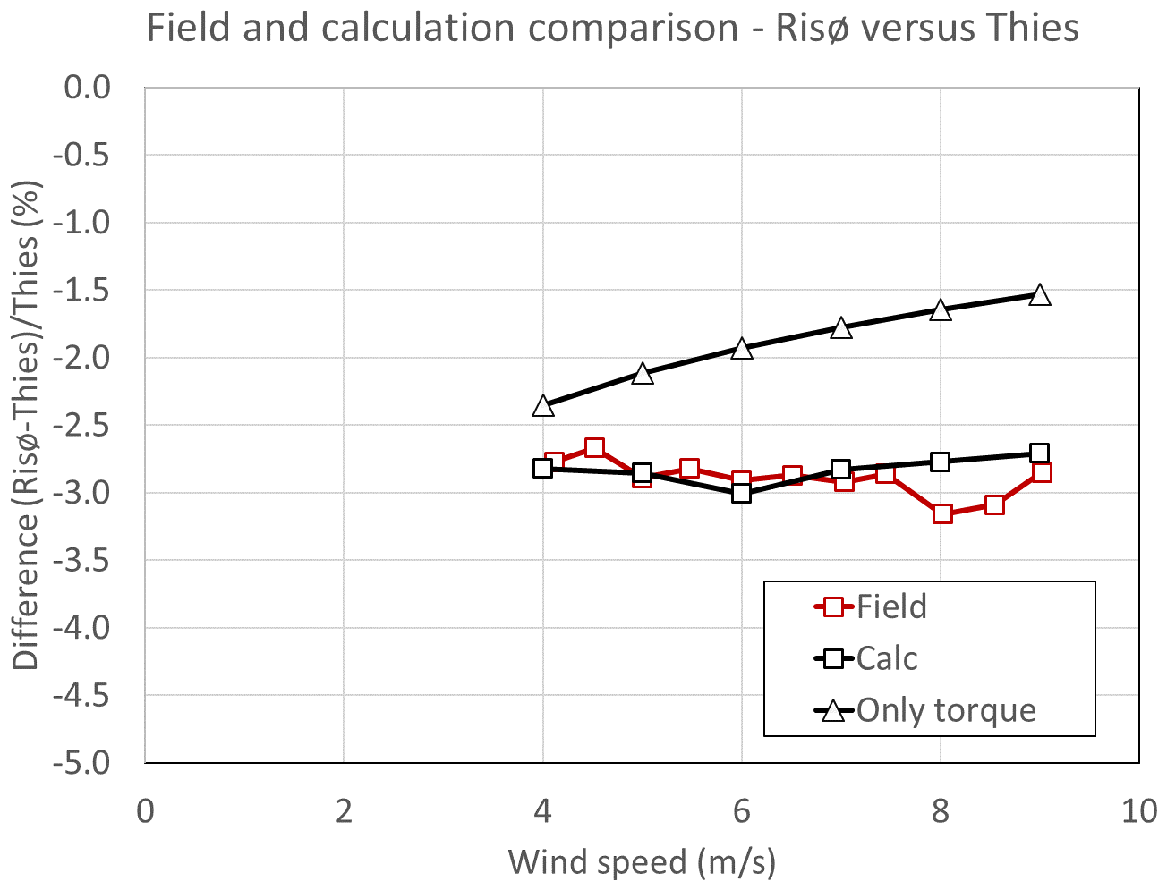
Figure 20Differences between Thies and Risø cup anemometers from the field comparison in Fig. 1, and with two ACCUWIND calculations: one with all influence parameters and one where only torque is considered.
The field comparison of the Thies and Risø cup anemometers in Fig. 1, which early demonstrated the problems of cup anemometer deviations, is in Fig. 20 supplemented with calculations. The calculations are made with a length scale Lu=100 m due to low height at 8 m, and with turbulence values from 0.36 at 4 m s−1 to 0.31 at 8 m s−1. More detailed knowledge of the field conditions was not available. The contribution from torque characteristics is in this comparison significant due to the higher-frequency content in the wind spectrum, due to the low height.
In order to improve the torque characteristics to reduce the overspeeding effect, we can start to look at the torque coefficient curves of Risø and Thies from Fig. 5 in the most relevant speed ratio range and normalize both curves with the speed ratio to the equilibrium speed ratio 0.3 (see Fig. 21). An improvement of the Risø torque characteristics could aim for the 0.26–0.34 curve (also shown in Fig. 21). We see that, below equilibrium speed ratio, where cup rotors accelerate, they almost fall on one line with the same slope, except for the 0.24–0.36 curve. This part of the curves differ significantly from the parabolic model curves in Fig. 10 and the partial linear model in Fig. 12, which spread quite a bit. The torque coefficient curves above the equilibrium speed ratio, where cup rotors decelerate, spread significantly with steeper slopes for reduced overspeeding. This indicates that the overspeeding effect could be reduced by further increasing the low drag coefficient, as Brevort and Joyner (1934) found when going from a hemispherical cup (CDL=0.40) to a conical cup (CDL=0.48), while the high drag coefficient is the same for both (CDL=1.40) (Brevort and Joyner, 1934). We cannot, however, use the drag model theory to improve on the overspeeding, though the drag model is the only model which uses aerodynamic characteristics of the cup rotor in the torque coefficient expression (CDH and CDL). One could be tempted to increase the low drag coefficient further. Increasing the low drag coefficient by 10 % would increase the drag ratio, k, by 10 % and reduce the equilibrium speed ratio by 8 % (Eq. 23). The calibration gain would be increased by 8 % (Eq. 10) because the rotor would run slower, and the maximum overspeeding would be reduced by less than 2 % (Eqs. 23 and 24). The maximum overspeeding would for a further increase of the low drag coefficient converge towards the linear maximum overspeeding (turbulence intensity squared) and the drag model cannot provide a lower value for any drag ratio. To reduce the overspeeding effect, it is necessary to consider the lift and drag interaction over the whole revolution, including the flow in the 120° wake sector where one cup is in the wake of the other two. Investigations on such detailed complex flows in order to optimize torque characteristics have so far not been made.
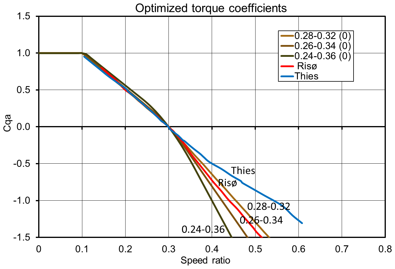
Figure 21Torque coefficient curves for optimized torque with constants CQA0=1.5, λ0=0.3, and λ1=0.0, three parabolic ranges (0.24–0.36 (light beige), 0.26–0.34 (medium beige), and 0.28–0.32 (dark beige)), and added Risø (red) and Thies (blue) torque coefficient curves, normalized to speed ratio λ0=0.3.
Within the last decades, research on cup anemometer characteristics was taken to a new level within the wind energy community. A historical review showed the need for improved models and methods for cup anemometer uncertainty analysis. The development of improved cup anemometer models and classification methods was triggered by the measurement uncertainty requirements for power performance measurements on wind turbines. Results of the research are now implemented in the IEC standards on power performance measurements, including the updated standards.
Inter-calibration of cup anemometers between European test stations revealed variations of up to 10 % between wind tunnel calibrations. However, European cooperation has today led to variations below 0.5 % within the MEASNET measurement organization.
Assessments of cup anemometers by field comparisons showed variations of several percent, and the cause was found to be significantly dependent on turbulence intensity. European research projects (SITEPARIDEN, CLASSCUP and ACCUWIND) investigated the causes and found angular characteristics and dynamic response to be the main causes. Methods for assessment of characteristics (and models for systematic simulation of responses) and a classification method were developed. Cup anemometer models developed from research within the meteorology community were found, but no strict requirements or methods for field measurement uncertainty was found.
The found cup anemometer models were the two-cup drag model, parabolic models, perturbation models, a phenomenological forcing model and linear models. All of the models were investigated and compared, in order to find an appropriate simulation model for uncertainty estimation and classification. None of the models fitted actual torque data accurate enough, and a new ACCUWIND model was developed, which uses tabulated data instead of mathematical formulae.
Wind tunnel measurements analysed angular and dynamic response and found severe variations between commercial cup anemometer models. Dynamic response was investigated in wind tunnel with torque sensor measurements, and overspeeding was measured with sinusoidally varying wind in the wind tunnel. Very low overspeeding and even slightly negative overspeeding were experienced. Maximum overspeeding as a function of turbulence intensity and step responses from below and above was found to express the dynamic response in a clear way.
The comparison of models showed that the often referenced drag model always led to systematic high maximum overspeeding of about 1.1 times turbulence intensity squared, which, however, is not present in modern cup anemometers with conical cups. The model fitted, approximately, to an older cup anemometer type with hemispherical cups. The more general parabolic model showed that maximum overspeeding can be zero or slightly negative at low or medium turbulence intensities. A new cup anemometer model with optimized zero maximum overspeeding was developed, and a conical cup anemometer type was found to fit approximately to the model. The linear torque coefficient model provides maximum overspeeding by the turbulence intensity squared. The partial linear model showed that torque characteristics can be measured with step responses from below and above. Such characteristics can approximately provide the same classification results as the ACCUWIND model with tabulated data.
When the models are exposed to a wind spectrum, the overspeeding is significantly reduced compared to the maximum overspeeding. This is due to relatively low rotor inertia. The drag model shows the highest overspeeding, but the model is also significantly overestimating the overspeeding of the conical cup rotor.
Classification results with only torque characteristics (no friction, no angular response) show similar low overspeeding results. Classifications of the Risø and Thies cup anemometers show significantly higher values when angular response and friction are included.
The ACCUWIND model and the classification method are described in detail in the IEC power performance standards. A model example calculation with an Anemcq7.exe code (available from the author) is provided in the standard.
TFP contributed with theoretical work, and he wrote the article. JÅD contributed with experimental wind tunnel work, with evaluation of results, discussions and review of the article.
TFP worked for decades on power performance measurements with the Risø cup anemometer, which was developed and improved at Risø (now DTU) by meteorologists and later by Ole Frost Hansen, to whom the design and production was outsourced in 2006 to the spin-off company WindSensor. Both authors participated in the CLASSCUP and ACCUWIND projects and were members of the IEC standardization committee that adopted the ACCUWIND classification method.
Publisher’s note: Copernicus Publications remains neutral with regard to jurisdictional claims made in the text, published maps, institutional affiliations, or any other geographical representation in this paper. While Copernicus Publications makes every effort to include appropriate place names, the final responsibility lies with the authors.
The research work was supported by the European Commission with two European projects: CLASSCUP (contract no. JOR3-CT98-0263) and ACCUWIND (contract no. NNE5-2001-00831).
This paper was edited by Laura Bianco and reviewed by Daniel Alfonso-Corcuera and one anonymous referee.
Albers, A.: Open field cup anemometry, DEWI Magazin Nr. 19, 53–58, 2001.
Albers, A., Klug, H., and Westermann, D.: Cup anemometry in Wind Engineering, Struggle for improvement, DEWI Magazin Nr. 18, 17–28, 2001.
ASTM: Standard test method for determining the performance of a cup anemometer or propeller anemometer, ASTM International, West Conshohocken, PA, https://doi.org/10.1520/D5096-17, 2017.
Barton, S.: Evaluation of distance constants for various cup anemometers and measurement of the vertical sensitivity of a 'Vector' type A100 cup anemometer, Report No 421/88, National Engineering Laboratory, https://orbit.dtu.dk/en/publications/ evaluation-of-distance-constaints-for-various-cup-anemometers-and (last access: 8 February 2024), 1989.
BIPM, IEC, IFCC, ILAC, ISO, IUPAC, IUPAP, and OIML. Evaluation of measurement data | Guide to the expression of uncertainty in measurement, Joint Committee for Guides in Metrology, JCGM 100:2008, https://www.bipm.org/documents/20126/2071204/JCGM_100_2008_E.pdf/cb0ef43f-baa5-11cf-3f85-4dcd86f77bd6 (last access: 8 February 2024), 2008.
Brevort, M. J. and Joyner, U. T.: Experimental investigation of the Robinson-type cup anemometer, NACA, Report No. 513, https://ntrs.nasa.gov/citations/19930091586 (last access: 8 February 2024), 1934.
Busch, N. E. and Kristensen, L.: Cup Anemometer Overspeeding, J. Appl. Meteorol., 15, 1328–1332, https://doi.org/10.1175/1520-0450(1976)015<1328:CAO>2.0.CO;2, 1976.
Cleveland, A.: Meteorological Apparatus and Methods: Annual report of the chief signal officer of the army, Washington, 1887, appendix 46, https://babel.hathitrust.org/cgi/pt?id=njp.32101072897281&seq=11 (last access: 8 February 2024), 1888.
Coppin, P. A.: An examination of cup anemometer overspeeding, Meteorological Research, 35, 1–11, 1982.
Dahlberg, J. A., Gustavsson, D. J., Ronsten, G., Pedersen, T. F., Paulsen, U. S., and Westermann, D.: Development of a standardised cup anemometer suited to wind energy applications – CLASSCUP, Aeronautical Research Institute of Sweden, Stockholm, FOI-S-0108-SE, https://doi.org/10.11581/DTU.00000309, 2001.
Dahlberg, J. A., Pedersen, T. F., and Busche, P.: ACCUWIND - Methods for classification of cup anemometers, Risø National Laboratory, Roskilde, Risø-R-1555, ISBN 87-550-3514-0, 2006.
Eecen, P. J., Cuerva, F., and Mouzakis, A.: ACCUWIND, Work Package 3 Final Report, ECN-C-06-047, ECN, https://publicaties.ecn.nl/ECN-C--06-047 (last access: 8 February 2024), 2006.
Fabian, O.: Fly-wheel calibration of cup anemometers, in: Proceedings EWEC Thessaloniki 1995 Contributions from the Department of Meteorology and Wind Energy to the EWEC'94 conference in Thessaloniki, Greece, Risø-R-797, 29–33, https://orbit.dtu.dk/en/publications/contributions-from- the-department-of-meteorology-and-wind-energy–3 (last access: 8 February 2024), 1995.
Hoerner, F. S.: Fluid Dynamic Drag, Hoerner Fluid Dynamics, Bricktown, New Jersey, 3–17, https://archive.org/details/FluidDynamicDragHoerner1965/page/n59/mode/2up (last access: 8 February 2024), 1965.
HMSO: Handbook of Meteorological Instruments, second edition, Vol. 4, Measurement of Surface Wind, HMSO, London, 4–8, https://digital.nmla.metoffice.gov.uk/IO_39bf894f-96ad-4776-bdf0-dc43a4d54dd1/ (last access: 8 February 2024), 1981.
Hunter, R.: A comparison of cup anemometer calibrations, CEC Contract No 87-B-7010-11-7-17, https://doi.org/10.11581/DTU.00000307, 1989a.
Hunter, R.: Recommendations on the use of cup anemometry at the European Community wind turbine test stations, CEC Contract No 87-B-7010-11-7-17, https://doi.org/10.11581/DTU.00000308, 1989b.
Hunter, R. S., Pedersen, B. M., Pedersen, T. F., Klug, H., Borg, N. V. D., Kelley, N., and Dahlberg, J. Å. (Eds.): Recommended practices for wind turbine testing and evaluation. 11. Wind speed measurement and use of cup anemometry. 1. edition, IEA, https://orbit.dtu.dk/en/publications/recommended- practices-for-wind-turbine-testing-and-evaluation-11- (last access: 8 February 2024), 1999.
IEC-12: Wind energy generation systems – Part 12-1: Power performance measurements of electricity producing wind turbines - Overview, IEC 61400-12:2022, ISBN 978-2-8322-5621-3, https://webstore.iec.ch/publication/69211 (last access: 8 February 2024), 2022.
IEC-12-1: Wind energy generation systems - Part 12-1: Power performance measurements of electricity producing wind turbines, IEC 61400-12-1:2005, ISBN 2-8318-8333-4, 2005.
IEC-12-1: Wind energy generation systems - Part 12-1: Power performance measurements of electricity producing wind turbines, IEC 61400-12-1:2017, ISBN 978-2-8322-3823-3, 2017.
IEC-50-1: IEC 61400-50-1 ED1, Wind energy generation systems - Part 50-1: Wind measurement - Application of meteorological mast, nacelle and spinner mounted instruments, ISBN 978-2-8322-5937-5, 2022.
ISO: Meteorology – Wind Measurements – Part 1: Wind tunnel test methods for rotating anemometer performance, ISO 17713-1, https://www.iso.org/standard/31497.html (last access: 8 February 2024), 2007.
Kristensen, L.: Cup Anemometer Behaviour in Turbulent Environments, J. Atmos. Ocean. Tech., 15, 5–17, https://doi.org/10.1175/1520-0426(1998)015<0005:CABITE>2.0.CO;2, 1998.
Kristensen, L.: Can a cup anemometer underspeed, Bound.-Lay. Meteorol., 103, 163–172, 2002.
MacCready, P. B.: Dynamic response characteristics of meteorological sensors, B. Am. Meteorol. Soc., 46, 533–538, 1965.
Mann, J.: The spatial structure of neutral atmospheric surface-layer turbulence, J. Fluid Mech., 273, 141–168, 1994.
Mann, J.: Wind field simulation, Probabilist. Eng. Mech., 13, 269–282, 1998.
MEASNET: http://www.measnet.com/ (last access: 11 January 2024), 2023.
Papadopoulos, K. H., Stefanatos, N. C., Paulsen, U. S., and Morfiadakis, E.: Effects of turbulence and flow inclination on the performance of cup anemometers in the field, Bound.-Lay. Meteorol., 101, 77–107, 2001.
Pedersen, T. F.: Characterisation and Classification of RISØ P2546 Cup Anemometer, Risø National Laboratory, Roskilde, Risø-R-1364, ISBN 87-550-3112-9, 2004.
Pedersen, T. F.: Quantification of linear torque characteristics of cup anemometers with step responses, Risø DTU, Roskilde, Risø-I-3131(EN), https://doi.org/10.11581/DTU.00000310, 2011.
Pedersen, T. F. and Paulsen, U. S.: A Procedure for Classification of Cup-Anemometers, in: EWEC '97, European Wind Energy Conference, Dublin, Ireland, 6–9 October 1997, Irish Wind Energy Association, https://orbit.dtu.dk/en/publications/a-procedure-for-classification-of-cup-anemometers-2 (last access: 8 February 2024), 1997.
Pedersen, T. F. and Paulsen, U. S.: Classification of operational characteristics of commercial cup-anemometers, in: Wind energy for the next millennium, EWEC'99, Proceedings, Nice, France, 1–5 March 1999, edited by: Petersen, E. L., Hjuler Jensen, P., Rave, K., Helm, P., and Ehmann, H., James and James Science Publishers, 611–615, 1999.
Pedersen, T. F., Petersen, S. M., and Vølund, P.: Description and measurements of the wind that drives the power performance and mean loads of wind turbines, in: 1996 European Wind Energy Conference and Exhibition, Proceedings, Göteborg, Sweden, 20–24 May 1996, edited by: Zervos, A., Ehmann, H., and Helm, P., H.S. Stephens and Associates, 1016–1019, 1996.
Pedersen, T. F., Gjerding, S., Ingham, P., Enevoldsen, P., Hansen, J. K., and Jørgensen, H. K.: Wind Turbine Power Performance Verification in Complex Terrain and Wind Farms, Risø National Laboratory, Roskilde, Risø-R-1330, ISBN 87-550-3028-9, 2002.
Pedersen, T. F., Dahlberg, J.-Å., and Busche, P.: ACCUWIND – Classification of Five Cup Anemometers According to IEC61400-12-1, Risø National Laboratory, Roskilde, Risø-R-1556, ISBN 87-550-3516-7, 2006.
Pindado, S., Cubas, J., and Sorribes-Palmer, F.: The Cup Anemometer, a Fundamental Meteorological, Sensors, 14, 21418–21452, 2014.
Sanz-Andrés, Á., Pindado, S., and Sorribes, F.:, Mathematical analysis of the effect of rotor geometry on cup anemometer response, Sci. World J., 2014, 537813, https://doi.org/10.1155/2014/537813, 2014.
Scrase, F. J. and Sheppard, P. A., The Errors of Cup Anemometers in Fluctuating Winds, J. Sci. Instrum., 21, 160–161, 1944.
Schrenk, O.: Über die tragfähigkeitsfehler des Schalenkreutz Aanemometers bei schwankender Windstärke, Z. Tech. Phys., 10, 57–66, 1929.
Waldo, F.: Modern meteorology, chapter II Apparatus and Methods, Walter Scott, Charles Scribner's Sons, Broadway, New York, USA, 1893.
Westermann, D.: Overspeeding – über das eigentümliche Tiefpassverhalten von Schalensternanemometern, DEWI Magazin, 9, 56–63, 1996.
WMO: WMO-8: Guide to Meteorological Instruments and Methods of Observation, World Meteorological Organization, Geneva, WMO-No. 8, p. 168, ISBN 978-92-63-10008-5, 2014.
Wyngaard, J. C.: Cup, propeller, vane, and sonic anemometers in turbulence research, Annu. Rev. Fluid Mech., 13, 399–423, https://doi.org/10.1146/annurev.fl.13.010181.002151, 1981.
Wyngaard, J. C., Bauman, J. T., and Lynch, R. A.: Cup anemometer dynamics, in: Flow: Its measurement and control in science and industry, Part 2, Instrument Society of America, 1, 701–708, 1974.
- Abstract
- Introduction
- Verification of differences in characteristics of cup anemometers
- Assessment of cup anemometer characteristics
- Cup anemometer models
- Overspeeding characteristics derived from cup anemometer models
- Step responses derived from cup anemometer models
- Distance constant
- Optimized torque characteristics
- Conclusions
- Code and data availability
- Author contributions
- Competing interests
- Disclaimer
- Financial support
- Review statement
- References