A novel infrared imager for studies of hydroxyl and oxygen nightglow emissions in the mesopause above northern Scandinavia

The paper describes technical characteristics and presents the first scientific results of a novel infrared imaging system (imager) for studies of nightglow emissions coming from the hydroxyl (OH) and molecular oxygen (O₂) layers in the mesopause region (80–100 km) above northern Scandinavia. The OH imager was put into operation in November 2022 at the Swedish Institute of Space Physics in Kiruna (67.86° N, 20.42° E; 400 m altitude). The OH imager records selected emission lines in the OH(3-1) band near 1500 nm to obtain intensity and temperature maps at around 87 km altitude. In addition, the OH imager registers infrared emissions coming from the O₂ IR A-band airglow at 1268.7 nm in order to obtain O₂ intensity maps at a slightly higher altitude, around 94 km. This technique allows the tracing of wave disturbances in both horizontal and vertical domains in the mesopause region. Validation and comparison of the OH(3-1) rotational temperature with collocated lidar and Aura Microwave Limb Sounder (MLS) satellite temperatures are performed. The first scientific results obtained from the OH imager for the first winter season (2022–2023) are discussed.

1 Introduction

Aside from a well-known scattering of sunlight on air molecules (Rayleigh scattering) and particle scattering, the Earth's atmosphere emits its own radiation 24 h d⁻¹, year-round and on global scales. So-called airglow emissions occur in the mesosphere (50–90 km) and thermosphere (above 90 km). The most prominent airglow emissions are red and green lines of atomic oxygen, ultraviolet and infrared bands of molecular oxygen, hydroxyl (OH) emissions in the infrared part of the spectrum, the yellow emission line of sodium (Na), and ultraviolet and infrared bands of nitric oxide (NO) (e.g., Chamberlain, 1961; Khomich et al., 2008; Savigny, 2017).

Studies of airglow emissions provide important sources of information on the physical and chemical states of the middle and upper atmosphere. In particular, the temperature of emission layers in the middle and upper atmosphere can be determined by analyzing spectral bands and lines of airglow emissions. By analyzing spatial–temporal variations in the emission intensities and/or temperature, one can investigate the short- and long-term dynamical state of the middle and upper atmosphere, which in turn is a hot topic of current atmospheric research (e.g., Fritts and Alexander, 2003; Plougonven and Zhang, 2014; Reid et al., 2014; Wüst et al., 2023; Gavrilov et al., 2024). The key role in the atmospheric dynamical state belongs to waves, a fundamental property of the atmosphere as they transport energy and momentum across great distances (Gossard and Hook, 1975).

Observations of airglow emissions are used to infer parameters of atmospheric waves since temperature and emission intensity fields in the mesosphere and thermosphere are directly modulated by gravity and planetary waves, solar thermal tides and lunar gravitational tides (e.g., Garcia et al., 1997; Taylor et al., 1997; Pautet et al., 2005; Suzuki et al., 2008; Offermann et al., 2009; Gao et al., 2011; Perminov et al., 2018; Pertsev et al., 2021).

Another very important aspect of atmospheric physics is the long-term monitoring of atmospheric parameters. The scientific community is debating to what extent long-term changes in H₂O, CO₂, N₂O, CH₄ and O₃ (greenhouse gases of anthropogenic and natural origin) contribute to long-term variability in atmospheric temperature. While CO₂ is thought to add to global warming on Earth, it also cools the middle atmosphere (Roble and Dickinson, 1989; Mlynczak et al., 2022). The increased H₂O concentration leads to warmer temperatures due to strong positive water vapor feedback (Dessler et al., 2008). Methane oxidizes in the stratosphere and mesosphere, producing an additional amount of water vapor in the middle atmosphere (Thomas and Olivero, 2001). The global monthly mean atmospheric-methane abundance demonstrates a constant increase since 1987 (https://gml.noaa.gov/ccgg/trends_ch4/, last access: 27 February 2024), which may have caused the observed long-term trend in water vapor in the mesopause. Lübken et al. (2018) have obtained a summer mesopause cooling of ∼ 1.2 K per decade for the period of 1960–2008 based on Leibniz Institute Middle Atmosphere (LIMA) and Mesospheric Ice Microphysics And tranSport (MIMAS) model simulations which included long-term evolutions of the minor atmospheric species CO₂, CH₄, H₂O and O₃. Thus, the long-term temperature trend in the middle atmosphere is a complex function of several atmospheric components. Estimates of temperatures of the middle atmosphere are only possible with the help of remote-sensing instruments. That is why observations of airglow emissions are used for long-term monitoring of the temperature in the mesopause region (Semenov and Shefov, 1999; Espy and Stegman, 2002; Offermann et al., 2010; Ammosov et al., 2014; Kalicinsky et al., 2016; Perminov et al., 2018; Dalin et al., 2020; French et al., 2020).

More than 50 sites conducting spectroscopic and imaging airglow observations are presented at the Network for the Detection of Mesospheric Change (NDMC), which is a global program investigating climate change signals in the mesopause region (https://ndmc.dlr.de/, last access: 27 February 2024). Li et al. (2018) have summarized a global distribution of all-sky airglow imager sites (see Table 1 in their paper and references therein). Some of the OH spectrographs and imaging instruments have a narrow field of view of 30° or less, such as the Ground-based Infrared P-branch Spectrometer instrument (GRIPS 6) in Oberpfaffenhofen, Germany (Schmidt et al., 2013); the Aerospace Nightglow Imager 2 (ANI2) in the Andes, Chile (Hecht et al., 2023); and the spectral airglow temperature imager (SATI) in Resolute Bay, Canada (Wiens et al., 1997). A number of OH imaging instruments measure OH emissions in relative units without mesopause temperature derivations, such as the ANI2; the OH all-sky airglow imager in Kazan, Russia (Li et al., 2018); and the Fast Airglow IMager (FAIM) in Oberpfaffenhofen, Germany (Hannawald et al., 2016). Some of the OH imagers register OH emissions (including temperature derivations) without capturing infrared emissions coming from the O₂ layer, such as the Advanced Mesospheric Temperature Mapper (AMTM) at the South Pole (Pautet et al., 2014) and the Near InfraRed Aurora Camera (NIRAC) in Svalbard, Norway (Nishiyama et al., 2024).

Table 1 The main characteristics of the OH imager in Kiruna.

In the present paper, we describe a novel wide-angle infrared imaging instrument (referred to hereafter as the OH imager) capable of registering emissions coming from two emitted layers (OH and O₂) and of deriving the mesopause temperature. The OH imager is the first of its kind installed in northern Scandinavia. The instrument measures infrared emissions of selected lines in the OH(3-1) band at wavelengths near 1.5 µm to produce intensity and temperature maps in the mesopause region at around 87 km altitude. Additionally, the OH imager records nightglow emissions from the O₂ IR A-band at 1268.7 nm to obtain O₂ emission intensity maps at a slightly higher altitude of about 94 km. Combining data from both layers allows the tracing of wave disturbances in 3-D space, i.e., horizontally and vertically in the mesopause region. The OH imager was installed in November 2022 at the Swedish Institute of Space Physics (IRF) in Kiruna (67.86° N, 20.42° E; 400 m altitude) on the eastern side of the Scandinavian Mountains. Mountain gravity waves occur frequently at the location; thus the OH imager can be utilized to study the influence of such waves on the thermal and dynamical regime of the mesopause region over Kiruna. The OH registrations are part of the long-term research infrastructure commitment of the Kiruna Atmospheric and Geophysical Observatory (KAGO), part of the IRF, whose objective is to provide present and future scientists with long, continuously archived time series of data of the highest possible scientific quality from its set of instruments.

In Sect. 2, we describe the technical characteristics of the OH imager as well as the principle of OH(3-1) rotational temperature measurements. In Sect. 3, the temperature estimation and its uncertainty, calibration, and validation techniques are presented. Validation of OH(3-1) temperatures with the collocated Esrange lidar temperature measurements and a comparison of OH temperatures with simultaneous Aura Microwave Limb Sounder (MLS) satellite temperatures are shown in Sect. 4. In Sect. 5, the first scientific results obtained with the OH imager are discussed. Finally, conclusions are given in Sect. 6.

2 Instrument description

2.1 Theory and basic knowledge

The hydroxyl (OH) airglow emission layer exists in the Earth's atmosphere between 75 and 100 km, with the highest concentration at about 87 km and the full width at half maximum of about 8–10 km (Baker and Stair, 1988; Savigny, 2017), although both of these parameters of the OH-layer change depending on geolocation and season (Perminov et al., 1999, 2018; Melo et al., 2000; Grygalashvyly et al., 2014). Its rotational–vibrational bands, covering the spectral region from 0.5 to 4.5 µm, result mainly from the chemiluminescent processes (Bates and Nicolet, 1950):

$$\begin{array}{c}{\displaystyle }\mathrm{O}+{\mathrm{O}}_{\mathrm{2}}+M\to {\mathrm{O}}_{\mathrm{3}}+M,\\ {\displaystyle }{\mathrm{O}}_{\mathrm{3}}+\mathrm{H}\to {\mathrm{OH}}^{*}+{\mathrm{O}}_{\mathrm{2}}+\mathrm{3.3}\mathrm{eV},\end{array}$$

where M is a molecule of nitrogen or oxygen and OH^* is the OH vibrationally excited molecule. Returning to their ground state, the OH^* molecules emit visible and infrared radiation in the spectral range between 500 and 4500 nm.

The OH(8-3) band at 732–742 nm and the OH(6-2) band at 830–845 nm, which are detectable by commercial CCD cameras, are commonly used in OH airglow observations. However, at high latitudes, auroral emissions (molecular and atomic oxygen lines between 730 and 845 nm) have stronger intensities than those of the OH airglow bands (Christensen et al., 1978; Sivjee et al., 1979). Therefore, measurements of OH nightglow emissions in the short-wave infrared range (SWIR) of the spectrum (900–1700 nm) are preferable in order to minimize auroral contamination at high latitudes (Pautet et al., 2014; Nishiyama et al., 2021). For this purpose, the OH(3-1) band (1470–1550 nm) is used by the OH imager to measure nightglow emissions at high latitudes. It is important to note that the OH(3-1) intensity is 2 orders of magnitude greater than the intensities of the OH(8-3) and OH(6-2) bands. Also, the OH(3-1) emission is less affected by water vapor absorption. All these factors make for a strong preference in choosing the OH(3-1) nightglow observation in Kiruna, as it is located underneath the auroral oval where auroral emissions occur frequently.

2.2 Instrument description

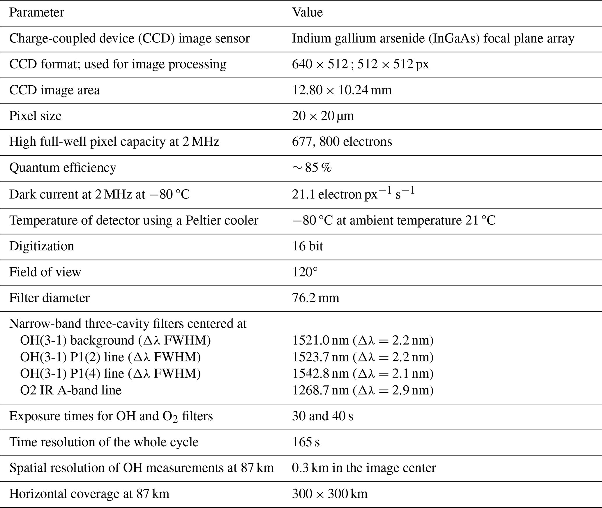
The main component of the OH imager is an infrared camera (Teledyne Princeton Instruments NIRvana 640) equipped with an indium gallium arsenide (InGaAs) sensor for low-light scientific SWIR imaging applications. The NIRvana 640 camera employs a 640 × 512 InGaAs array charge-coupled device (CCD), with a spectral response from 900 to 1700 nm. Each pixel has a size of 20 × 20 µm. The detector is Peltier-cooled to −80 °C to minimize thermally generated noise and thus improve the signal-to-noise ratio. The NIRvana 640 camera has 16-bit digitization, with low readout noise. Other components of the instrument are a SWIR wide-angle primary lens (∼ 120° field of view), an f/1.0 SWIR-optimized telecentric optical system, a thermally stabilized eight-position filter wheel with four narrow-band (three-cavity) interference filters, a brushless DC servo motor drive for the filter wheel, a filter wheel control unit, a power supply, and an instrument control and data acquisition computer. As the center wavelengths of the interference filters are temperature dependent, the filter wheel's closed-loop temperature controller heats the filter wheel cavity to +23 ± 0.1 °C. Along with four narrow-band interference filters, a dark-blocking filter is used to collect data for subtraction of dark-current noise from nighttime measurements. The dark-blocking filter's emissivity is matched to that of the narrow-band interference filters, thus ensuring the dark-current noise collected with it is representative of the dark-current noise present in nighttime measurements. The primary wide-angle lens, telecentric optics and reimaging lens were custom designed and produced for measurements in the SWIR. The reimaging optics consist of a doublet field lens and a combination of a second doublet and an f/1 compound lens in front of the sensor. The optical design of the OH imager inscribes a 120° field-of-view image circle within the short (vertical) dimension of the 640 × 512 px sensor, resulting in an image circle with a 512 px diameter. The image is therefore cropped to 512 × 512 px for image-processing purposes. The OH imager was designed and built by Keo Scientific Ltd (http://keoscientific.com, last access: 27 February 2024). The main instrument characteristics are summarized in Table 1.

Nightglow observations are restricted to nighttime and twilight (solar elevation angle less than −6.5°) for optimum signal quality. At the arctic location of Kiruna, we are thus able to conduct nightglow measurements from September until the middle of April. The exposure times for the OH, background and dark filters are set to 30 s, whereas the exposure time for the O₂ IR A-band filter is set to 40 s, yielding a complete filter cycle in 2.75 min. This yields the Nyquist frequency of the instrument equal to 0.019 s⁻¹ (5.5 min). To avoid aliasing with the Brunt–Väisälä frequency in the mesopause, which is varied around 0.021 s⁻¹ (5 min), the instrument is used to resolve the high-frequency range in the gravity-wave spectrum, corresponding to observed wave periods of about 10 min or more. Figure 1 shows the OH imager installed at the Knutstorp observatory (67.86° N, 20.42° E), 2 km north of IRF, on 29 November 2022.

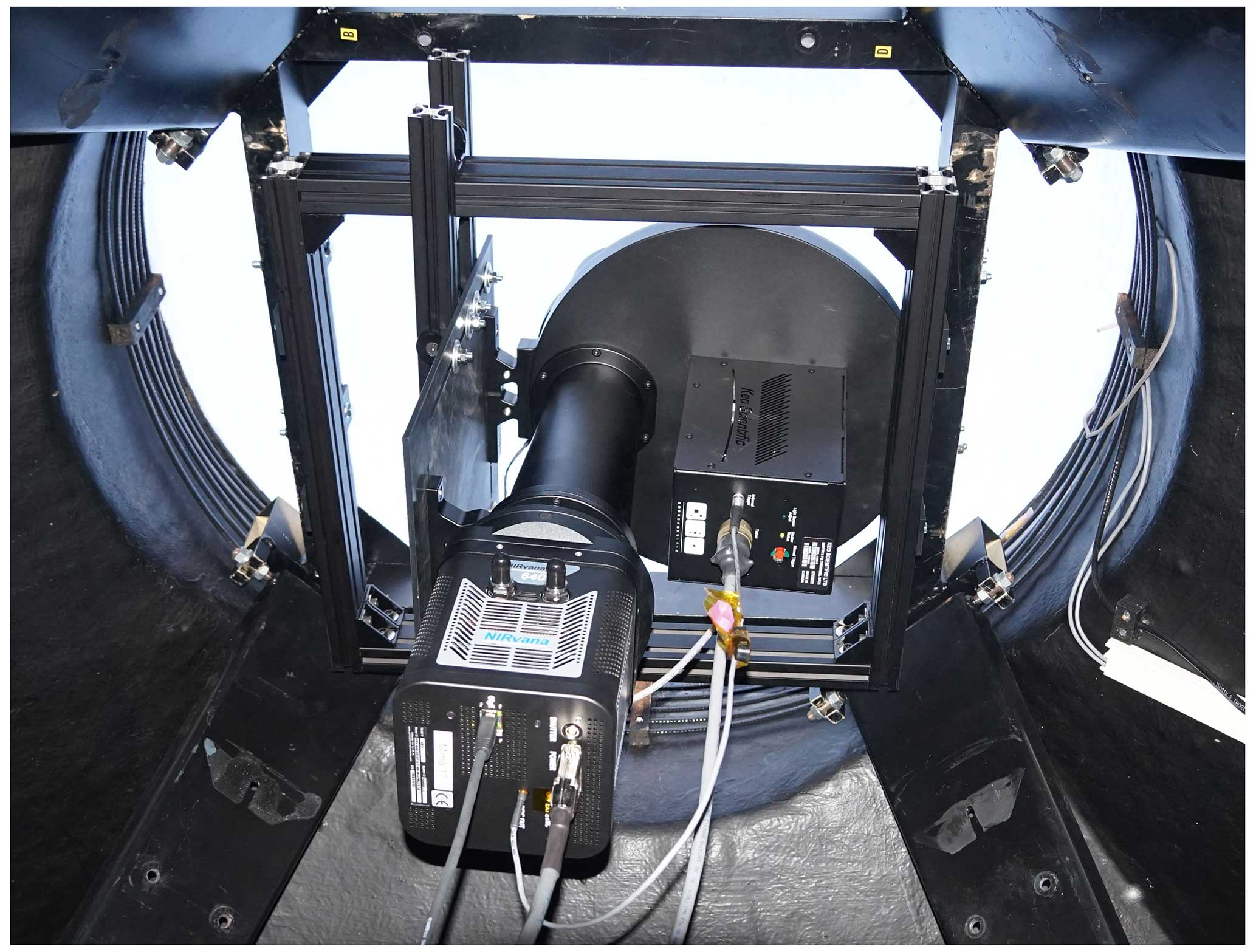
Figure 1 The Keo Scientific OH imager installed in November 2022 at the Swedish Institute of Space Physics (IRF) in Kiruna, Sweden (67.86° N, 20.42° E). The image was taken by Peter Dalin.

3 Temperature estimation and its uncertainty, error analysis, and calibration technique

3.1 Temperature estimation

The temperature of the air in the mesopause region is determined using the brightness ratio of the two vibrational-rotational lines P₁(2) and P₁(4) in the OH(3-1) band. This method is based on the assumption that the rotational level populations are in local thermodynamic equilibrium (LTE). Although the OH vibrational states are excited due to nonthermal processes, the rotational level population is still in LTE due to the long radiative lifetimes of vibrational states (e.g., Savigny, 2017). This method has been proved to be valid and has been applied for several decades in temperature measurements of the mesopause region (Sivjee and Hamwey, 1987; Makhlouf et al., 1995; Espy and Stegman, 2002; Pertsev and Perminov, 2008; Suzuki et al., 2008; Offermann et al., 2010; Grygalashvyly et al., 2014; Pautet et al., 2014; Kalicinsky et al., 2016; Perminov et al., 2018).

For the OH rotational temperature estimation, we use Eq. (4) from Pautet et al. (2014). At the same time, we have corrected this equation for the newly estimated Einstein A coefficients for the OH(3-1) band at the P₁(2) and P₁(4) lines as calculated by Brooke et al. (2016). The new A coefficients for the P₁(2) and P₁(4) lines are 9.895802 and 13.15222 s⁻¹, respectively. After correction for the A coefficients, the following equation for the OH rotational temperature estimation T_r is obtained:

$$\begin{array}{}\text{(1)}& T_{\mathrm{r}}={\displaystyle \frac{\mathrm{259.58}}{\ln \left(\mathrm{2.658}\cdot R\right)}},\end{array}$$

where R is the brightness ratio B(P₁(2)) $/B$(P₁(4)) inferred from measurements of the P₁(2) and P₁(4) lines in absolute units (rayleigh). Equation (1) differs from Eq. (4) by Pautet et al. (2014) in terms of the multiplier of the R parameter: 2.658 versus 2.644. This results in a 0.7–1.2 K temperature difference between temperature estimations in the present paper and Pautet et al. (2014), for a typical range of winter temperatures (180–240 K) in the mesopause region.

3.2 Absolute calibration

The purpose of the absolute calibration of the OH imager is to establish a relationship between the arbitrary, instrument-dependent raw pixel values (counts) and the column emission rate in units of rayleigh (R). Imager absolute calibration is a multistage process that was performed by Keo Scientific Ltd. First, bandpass-filter curves for the three OH(3-1) filters (atmospheric background, the P₁(2) line and P₁(4) line) were measured using a tunable SWIR laser. Second, on-axis broadband sensitivity was determined by imaging the output of a calibrated National Institute of Standards and Technology (NIST)-traceable integrating sphere through the imager, including the filters, and onto the InGaAs photodiode array sensor. Additionally, on-axis, “at-wavelength” sensitivity was measured for each filter using a collimated laser beam calibrated with a NIST-traceable optical power meter through the imager and onto the InGaAs photodiode array sensor. This resulted in the final absolute calibration coefficients, valid on-axis. Finally, a flat-field correction procedure was performed to compensate for off-axis vignetting, resulting in uniformity coefficients (one for each OH filter), allowing one to apply the absolute calibration coefficients to any pixel in the image. The flat-field correction consists of three steps: (1) the cylindrically symmetric component of the lenses is characterized first. This is done on an optical bench (180° rotary table) and an integrating sphere, where the sphere is illuminated with a tunable laser at the emission wavelengths of each of the two OH channels. (2) The imager is inserted into the integrating sphere and an additional diffuser is placed over the fisheye lens. Images are taken with the filters in place and with the uncoated glass blank in place. This is to find the attenuation of the filters relative to the uncoated glass blanks. (3) Zernike polynomials are then used for the fitting to produce the smooth flat fields. A calibration certificate with supporting files was issued by Keo Scientific.

3.3 Geometrical calibration

Geometrical calibration of the OH imager is a necessary procedure to measure the absolute horizontal coordinates of each pixel of the sensor at the instrument location. The geometrical calibration was performed by analyzing images of a clear night sky with reference stars using a wide-band filter (1000–1600 nm) in the filter wheel. The Positions and Proper Motions (PPM) Star Catalogue was used to identify the positions of the reference stars. The third-order polynomial P describes the camera optical model:

$$\begin{array}{}\text{(2)}& \begin{array}{rl}P& =a_{\mathrm{1}}\cdot x^{\mathrm{3}}+a_{\mathrm{2}}\cdot x^{\mathrm{2}}y+a_{\mathrm{3}}\cdot y^{\mathrm{2}}x+a_{\mathrm{4}}\cdot y^{\mathrm{3}}+a_{\mathrm{5}}\cdot x^{\mathrm{2}}\\ & +a_{\mathrm{6}}\cdot xy+a_{\mathrm{7}}\cdot y^{\mathrm{2}}+a_{\mathrm{8}}\cdot x+a_{\mathrm{9}}\cdot y+a_{\mathrm{10}},\end{array}\end{array}$$

where the 10 a_i parameters are free coefficients and x and y are the horizontal coordinates of the reference stars in the analyzed image. By comparing the theoretical horizontal coordinates of reference stars (more than 50 reference stars have been identified in reference images) with their measured coordinates, 10 free coefficients of the third-order polynomial were calculated using the least-squares method. These 10 coefficients describe all possible optical distortions in the whole camera optical path. This procedure finally resulted in the calculation of the absolute horizontal coordinates (elevation and azimuth angles) of each pixel, followed by a georeference procedure to project each pixel onto the Earth's surface. For this, the mean altitudes of the OH and O₂ layers were chosen as 87 and 94 km, respectively. The spatial horizontal resolution in the center of the image is about 0.3 km, reaching ∼ 1.2 km at the edges of the image.

3.4 Error analysis

In order to estimate the total error of temperature estimation, we need to rewrite the basic Eq. (1). The R brightness ratio in Eq. (1) depends on four variables represented by their raw measurement values in counts: the raw intensity of the P₁(2) line I_P12, the raw intensity of the P₁(4) line I_P14, the atmospheric background raw intensity I_bg and instrumental dark-current noise n_dc. The raw intensities I_P12 and I_P14 mean that no corrections for the atmospheric background and noise have been made. Thus, Eq. (1) can be rewritten in terms of these four variables as follows:

$$\begin{array}{}\text{(3)}& T_{\mathrm{r}}={\displaystyle \frac{\mathrm{259.58}}{\ln (\mathrm{2.658}\cdot \frac{k_{\mathrm{1}}\cdot k_{\mathrm{4}}\cdot \left(k_{\mathrm{2}}\cdot I_{\mathrm{P}\mathrm{12}}-k_{\mathrm{3}}\cdot I_{\mathrm{bg}}+\mathrm{0.22}\cdot n_{\mathrm{dc}}\right)}{k_{\mathrm{5}}\cdot k_{\mathrm{7}}\cdot \left(k_{\mathrm{6}}\cdot I_{\mathrm{P}\mathrm{14}}-k_{\mathrm{3}}\cdot I_{\mathrm{bg}}+\mathrm{0.60}\cdot n_{\mathrm{dc}}\right)})}},\end{array}$$

where k₁, k₂, k₃, k₄, k₅, k₆ and k₇ are the coefficients determined in the laboratory during the absolute calibration procedure. Equation (3) comes from Eq. (1) in the following way: the R brightness ratio in Eq. (1) is in absolute units (rayleigh). The instrument registers emission intensities (P₁(2), P₁(4) and atmospheric background) in relative digital units (counts). In order to relate relative to absolute units, the absolute calibration is performed. The main part of this procedure is to determine the absolute filter sensitivities that are different for each filter. These are the coefficients k₂, k₃ and k₆ in Eq. (3). In addition, the dark noise is subtracted both from the P₁(2) and P₁(4) lines and from the atmospheric background line, which, in turn, is finally subtracted from the P₁(2) and P₁(4) lines. Since the coefficients k₂, k₃ and k₆ are different, this procedure results in different constants (0.22 and 0.60) for the subtracted dark noise in the numerator and denominator in Eq. (3). These constants have positive signs since the dark noise is subtracted from the P₁(2) and P₁(4) lines and from the atmospheric background line with different coefficients. The coefficients k₄ and k₇ describe the flat field-correction factors as being different for each OH(3-1) emission line. Finally, the coefficients k₁ and k₅ convert photometric units to rayleigh, including several multipliers and the geometric etendue.

In order to estimate these four raw measurement values (I_P12, I_P14, I_bg and n_dc) and their errors, we follow the method proposed by Pautet et al. (2014). Measurements should be performed during a time when atmospheric and geomagnetic perturbations are at a minimum (i.e., only small variations in raw OH emission lines and in the atmospheric background, no contamination by tropospheric clouds, and no auroral emissions). A period of 1 h on 6 April 2023 was chosen to evaluate the four raw measurement variables and their errors. Figure 2 illustrates the raw intensities for the P₁(2) and P₁(4) lines as well as for the raw atmospheric background (BG) measured at the zenith over a single-pixel area (0.003 × 0.003°). To reduce measurement perturbations as much as possible, the raw data were smoothed using a three-point moving average. Then the residuals were determined by subtracting the smoothed curves from the raw intensity data, and their standard deviations were estimated. We obtained the following smoothed average values and their standard deviations: 57 711 ± 290 counts for the P₁(2) line, 48 552 ± 110 counts for the P₁(4) line and 31 301 ± 126 counts for the BG. The measured random temperature error (δT_m) is calculated using a general equation of error propagation in the case of a function having several variables (Taylor, 1997):

$$\begin{array}{}\text{(4)}& \mathit{\delta }{T}_{\mathrm{m}}=\sqrt{{\left({\displaystyle \frac{\partial T}{\partial I_{{\mathrm{P}}_{\mathrm{12}}}}}\mathit{\delta }{I}_{{\mathrm{P}}_{\mathrm{12}}}\right)}^{\mathrm{2}}+{\left({\displaystyle \frac{\partial T}{\partial I_{{\mathrm{P}}_{\mathrm{14}}}}}\mathit{\delta }{I}_{{\mathrm{P}}_{\mathrm{14}}}\right)}^{\mathrm{2}}+{\left({\displaystyle \frac{\partial T}{\partial I_{\mathrm{bg}}}}\mathit{\delta }{I}_{\mathrm{bg}}\right)}^{\mathrm{2}}},\end{array}$$

where $\partial T/\partial I_{{\mathrm{P}}_{\mathrm{12}}}$, $\partial T/\partial I_{{\mathrm{P}}_{\mathrm{14}}}$ and $\partial T/\partial I_{\mathrm{bg}}$ are the partial derivatives of T_r (see Eq. 3) with respect to raw intensity values P₁(2), P₁(4) and atmospheric background, respectively, and $\mathit{\delta }{I}_{{\mathrm{P}}_{\mathrm{12}}}$, $\mathit{\delta }{I}_{{\mathrm{P}}_{\mathrm{14}}}$ and δI_bg are their standard deviations. When inserting the parameters that were estimated above into Eq. (4), a temperature measurement random error of 1.80 K is derived.

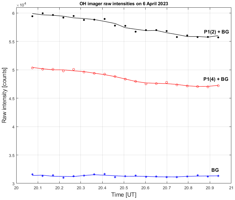
Figure 2 Raw intensities of emission lines at the zenith as measured by the OH imager in Kiruna on 6 April 2023. The black dots, red circles and blue asterisks are the raw intensities of the OH P₁(2), OH P₁(4) (including atmospheric background and noise level of the detector) and raw atmospheric background (BG) lines, respectively. The black, red and blue lines are three-point moving averages.

The temperature instrumental error is mainly governed by the dark-current noise of the CCD sensor and by the coefficients $k_{\mathrm{1},\mathrm{2},\mathrm{3},\mathrm{4},\mathrm{5},\mathrm{6},\mathrm{7}}$ in Eq. (3). The dark-current noise was continuously monitored using the dark-blocking filter as part of the measurement cycle (every 2.75 min) and was subsequently subtracted from the recorded raw intensity values of the OH and O₂ emission lines. An example of dark-current noise is shown in Fig. 3, demonstrating the linear stability of the dark-current noise during the night of 6–7 April 2023, with a small, statistically insignificant regression coefficient equal to 186 ± 355 counts d⁻¹. The mean value of the dark-current noise n_dc and its standard deviation δn_dc is 30 900 ± 183 counts for this night. The relative errors of the coefficients $k_{\mathrm{1},\mathrm{2},\mathrm{3},\mathrm{4},\mathrm{5},\mathrm{6},\mathrm{7}}$ were estimated to vary from 0.8 % to 4.2 % in the course of the absolute calibration, which results in temperature errors ranging from 0.1 to 2.1 K.

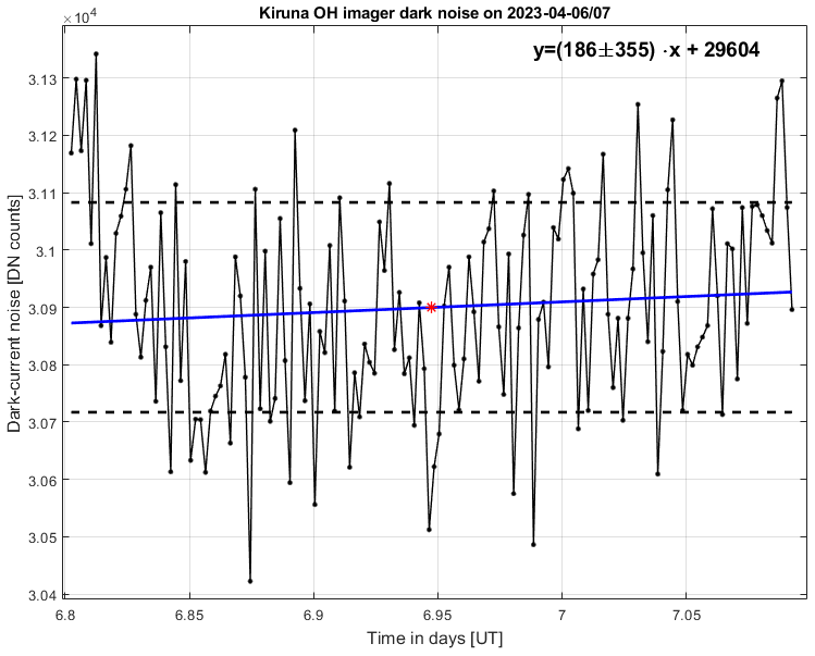
Figure 3 Example of the dark-current noise of the OH imager in Kiruna on the night of 6–7 April 2023. The black dots are dark-current noise counts in the detector center, the blue line is the linear regression, the red asterisk is the mean dark-current noise and the dashed lines are 1 standard deviation around the mean noise.

The total (instrumental and measurement) error δT_tot is calculated by adding the terms for the instrumental error to Eq. (4):

$$\begin{array}{}\text{(5)}& \begin{array}{rl}& \mathit{\delta }{T}_{\mathrm{tot}}=\\ & \sqrt{{\left({\displaystyle \frac{\partial T}{\partial n_{\mathrm{dc}}}}\mathit{\delta }{n}_{\mathrm{dc}}\right)}^{\mathrm{2}}+{\left({\displaystyle \frac{\partial T}{\partial k_i}}\mathit{\delta }{k}_i\right)}^{\mathrm{2}}+{\left({\displaystyle \frac{\partial T}{\partial I_{{\mathrm{P}}_{\mathrm{12}}}\mathit{\delta }{I}_{{\mathrm{P}}_{\mathrm{12}}}}}\right)}^{\mathrm{2}}+{\left({\displaystyle \frac{\partial T}{\partial I_{{\mathrm{P}}_{\mathrm{14}}}\mathit{\delta }{I}_{{\mathrm{P}}_{\mathrm{14}}}}}\right)}^{\mathrm{2}}+{\left({\displaystyle \frac{\partial T}{\partial I_{\mathrm{bg}}}}\mathit{\delta }{I}_{\mathrm{bg}}\right)}^{\mathrm{2}}},\end{array}\end{array}$$

where $\partial T/\partial n_{\mathrm{dc}}$ and $\partial T/\partial k_{i=\mathrm{1},\mathrm{2},\mathrm{3},\mathrm{4},\mathrm{5},\mathrm{6},\mathrm{7}}$ are partial derivatives of the temperature with respect to dark-current noise n_dc, and the coefficients $k_{i=\mathrm{1},\mathrm{2},\mathrm{3},\mathrm{4},\mathrm{5},\mathrm{6},\mathrm{7}}$, δn_dc and $\mathit{\delta }{k}_{i=\mathrm{1},\mathrm{2},\mathrm{3},\mathrm{4},\mathrm{5},\mathrm{6},\mathrm{7}}$ are their standard deviations. Based on the above estimated mean dark-current noise and its standard deviation, the mean temperature instrumental error due to dark-current noise is equal to 0.15 K on the night of 6–7 April 2023. The instrumental temperature error due to the coefficients $k_{\mathrm{1},\mathrm{2},\mathrm{3},\mathrm{4},\mathrm{5},\mathrm{6},\mathrm{7}}$ is equal to 3.37 K, and the total instrumental temperature error $\left(\sqrt{\left({\mathrm{0.15}}^{\mathrm{2}}+{\mathrm{3.37}}^{\mathrm{2}}\right)}\right)$ is 3.38 K. Finally, the resulting rotational temperature and its total error $\left(\sqrt{\left({\mathrm{1.80}}^{\mathrm{2}}+{\mathrm{3.38}}^{\mathrm{2}}\right)}\right)$ is equal to 193.9 ± 3.8 K for the particular case shown in Fig. 2.

At the same time, we should note that the actual variability of atmospheric conditions due to complex wave dynamics (turbulence, gravity and planetary waves, solar and lunar tides, and seasonal variations) is greater, resulting in an average standard deviation of the mesopause temperature above Kiruna of ∼ 10 K in 2023 (see Sect. 5). Most important is that the OH imager enables the resolution of small temperature variations of 4–6 K due to small-scale gravity waves, as will be demonstrated in Sect. 5.

4 Temperature validation and comparison

4.1 OH imager and lidar measurements

A Rayleigh–Mie–Raman backscatter lidar located at Esrange (∼ 40 km east of Kiruna) is used to validate the OH(3-1) temperatures as measured by the OH imager. The Esrange lidar was developed by Bonn University to monitor aerosols in the troposphere, stratosphere and mesosphere (Blum and Fricke, 2005). The signal from the aerosol-free part of the atmosphere can be used to determine the temperature, assuming atmospheric hydrostatic equilibrium. The vertical and time resolutions of the obtained measurements are 150 m and 4.2 min, respectively. We used a lidar backscattered signal from the 532 nm wavelength channel to calculate an atmospheric temperature profile above Esrange. Note that the temperature profile measured by the Esrange lidar is located in the field of view of the OH imager; i.e., common-volume simultaneous temperature measurements have been conducted to validate the OH(3-1) temperatures.

The Esrange lidar was operated when weather conditions were favorable during seven nights in the period from January to March 2023. An example of a temperature comparison, made on the night of 2–3 February 2023, between the OH imager and lidar is shown in Fig. 4. The OH temperature measurement has been selected from the temperature map as the one with the closest position to Esrange with 0.3 km uncertainty. At the upper end of the profile (at around 90 km), a seed temperature equal to 188 K was taken from Aura MLS satellite temperature measurements. The mean values of the OH(3-1) and lidar temperatures averaged for the time interval between 18:43 and 05:58 UTC on this night are presented. In addition, the lidar temperature profile has been smoothed using a 1.5 km running average in height in order to reduce large fluctuations in the upper part of the profile. The Aura MLS temperature profile with the closest position to Kiruna (about 420 km away) for this case is shown in Fig. 4 by the red line. Since the OH(3-1) temperature is measured across the whole OH layer between about 82 and 92 km, with a mean height of ∼ 87 km, for validation purposes the lidar temperature profile has been processed using a Gaussian function with the maximum at 87 km and with the full width at half maximum (FWHM) of 9.3 km height-weighted between 82 and 90 km, the same technique as was used by Pautet et al. (2014). The average height-weighted lidar temperature is equal to 191.8 ± 12.3 K, and the average OH(3-1) temperature is 193.6 ± 8.3 K. The temperature difference between these estimations is 1.8 K for this particular night, i.e., within the error margin. Following the same technique, we have made comparisons between the OH(3-1) and lidar temperatures for all seven available nights of simultaneous common-volume measurements, resulting in the following statistic: the average temperature difference, including the sign, between the OH imager and Esrange lidar is −0.2 ± 1.6 K. It means that, from a statistical point of view, the difference between the OH(3-1) and Esrange lidar temperatures is about zero. The maximum temperature difference between these instruments was −2.9 K on the night of 5–6 March 2023. Note that we estimate the Gaussian height-weighted lidar temperature between 82 and 90 km with the mean height of 87 km. However, the actual height distribution of the OH layer above Esrange is unknown since it varies, in general, in time and space (i.e., Pautet et al., 2014). Thus, one can conclude that there is good agreement between the OH(3-1) and Esrange lidar temperature measurements on individual nights (within 3 K) and on an average basis (close to zero), after taking into account the dynamical processes in the mesopause region and instrument errors.

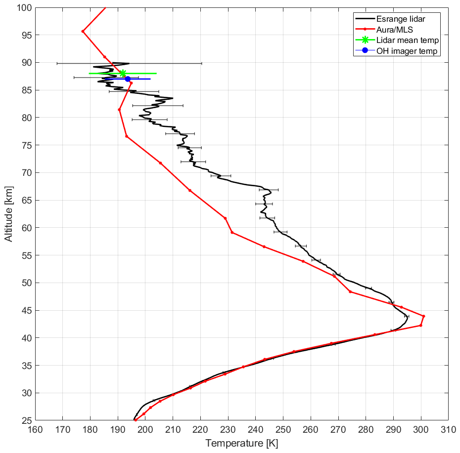
Figure 4 Temperature measurements made between 18:43 and 05:58 UTC on the night of 2–3 February 2023. The blue dot is the mean OH(3-1) temperature at 87 km averaged over the same time period. The black line is the Esrange lidar mean temperature profile. The green asterisk is the average height-weighted lidar temperature as calculated by vertical averaging across the OH layer (see text). Error bars for the OH imager and lidar measurements are 1 standard deviation of the temperature variations for the night. The red line is the Aura MLS temperature profile at 70.3° N, 12.2° E, closest to the position of Kiruna (about 420 km away), measured at 02:32 UTC on 3 February 2023.

4.2 OH imager and Aura MLS measurements

The Microwave Limb Sounder (MLS) radiometer on board the Aura satellite provides temperature profiles of the middle atmosphere with near-global coverage. Aura MLS temperature data (V5.0 and Level 2 data quality) can be obtained from the NASA public website: https://acdisc.gesdisc.eosdis.nasa.gov/data/Aura_MLS_Level2/ (last access: 28 February 2024). The description of MLS temperature retrieval and its validation can be found in Froidevaux et al. (2006) and Schwartz et al. (2008). We used Aura MLS temperature profiles as an additional way to compare temperatures that were retrieved with the OH imager.

The vertical resolution of Aura MLS temperature measurements is about 11–12 km in the mesopause region, and temperature precision of individual profiles is about 3.5 K at mesopause heights (see the Aura MLS data quality and description document available on the NASA website). Aura MLS temperatures at the pressure level of $\mathrm{4.6}\times {\mathrm{10}}^{-\mathrm{3}}$ hPa (about 86 km altitude) were chosen to be closest to the OH imager location (less than 300 km from Kiruna) and were measured simultaneously with OH(3-1) temperatures within the same hour. The comparison between OH imager and Aura MLS temperature measurements for the period January–April 2023 is illustrated in Fig. 5. In total, 22 individual temperature measurements have been collected. One can see that there are several cases in which the temperatures agree well within their uncertainties (days of the year 14, 58, 61, 65, 83, 85, 86, 92, 93, 99 and 101). For other days the agreement is worse. Note that even if the Aura MLS instrument measures temperature in the closest proximity to the OH imager, the Aura MLS horizontally scans a rather large volume of the mesopause (about 250–280 km) along its trajectory, which is not exactly the same mesopause volume as that which the OH imager measures; aside from this, the vertical resolution of Aura MLS temperature data in the mesopause is not equal to the width of the OH layer. All these factors complicate precise comparison. Natural variabilities of the atmosphere due to wave dynamics and chemical processes result in different temperatures in different atmospheric volumes. At the same time, two important conclusions can be drawn from Fig. 5: (a) there is no systematic bias (neither negative nor positive) in the OH(3-1) temperature relative to the Aura MLS temperature since there are OH(3-1) temperatures higher and lower than Aura MLS temperatures, and (b) the average temperature difference, including the sign, between the OH imager and Aura MLS is 2.8 ± 7.8 K. This is a small difference, taking into account the abovementioned limitations.

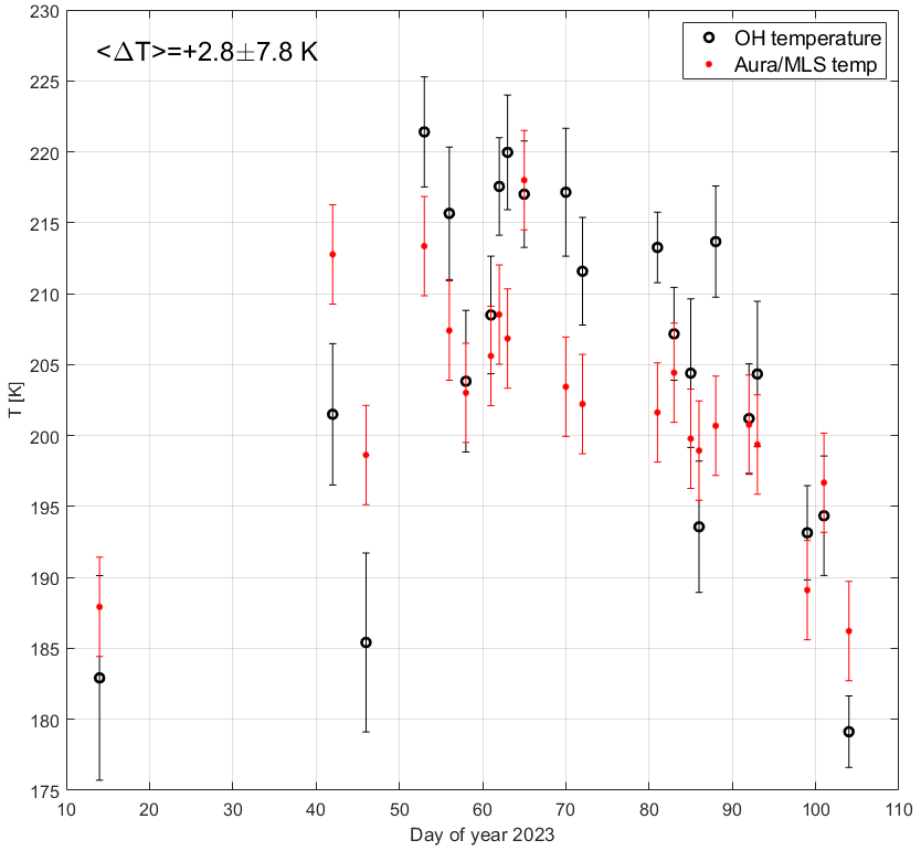
Figure 5 A comparison between simultaneous measurements of the mesopause temperature performed by the OH imager (black circles) above Kiruna at ∼ 87 km and by Aura MLS (red points) at 0.0046 hPa (∼ 86 km), close to the Kiruna location (distance difference is less than 300 km). Error bars of the OH(3-1) temperature are 1 standard deviation for a particular hour. Error bars of the Aura MLS temperature are equal to 3.5 K (see text).

5 Results and discussion

Maps of OH(3-1) intensities in rayleigh and O₂ IR A-band intensity in relative units, as well as the OH(3-1) temperature map on 16 February 2023, are illustrated in Fig. 6. One can see there is fine modulation of the temperature (Fig. 6d) due to small-scale gravity waves with wavelengths of 4–8 km overlying larger gravity-wave crests; the temperature amplitudes due to these small-scale waves are in the range of 4–6 K. It means that this case clearly demonstrates the ability of the OH imager to resolve small-amplitude, small-scale dynamical temperature variations that are important for studying the high-frequency range of the gravity-wave spectrum. Figure 7 illustrates a zoom of the images shown by the black squares in Fig. 6, which focuses on the small-scale wave structure of the approximately 4–6 km wavelength in the P₁(2), P₁(4) and temperature maps. Residuals of the P₁(2) and P₁(4) intensities are shown after subtraction of the mean intensity values from these zoomed-in images. Note that the temperature estimation (see Eq. 1) is not a linear function of the P₁(2) and P₁(4) line intensities, meaning that the linear scale of the P₁(2) and P₁(4) changes shown in Fig. 7a and b cannot directly represent the temperature changes in the observed small-scale wave structures shown in Fig. 7d. Another important feature of this case is that there is a medium-scale modulation, oriented in the direction from northwest to southeast, with horizontal wavelengths of 20–40 km and temperature amplitudes of 7–10 K. These medium-scale gravity-wave crests are clearly seen on all four maps, meaning that the same gravity-wave package was propagating through both the OH layer (maximum at ∼ 87 km) and the O₂ layer (maximum at ∼ 94 km). An analysis of the sequence of temperature maps has demonstrated that these medium-scale gravity waves were moving from southwest to northeast, with an observed horizontal-phase speed of about 30–35 m s⁻¹. This type of medium-scale gravity wave is common in the mesopause region (e.g., Pautet et al., 2011; Demissie et al., 2014). Thus, the OH imager allows the retrieval of information on gravity waves propagating in both horizontal and vertical domains in the mesopause region. A detailed analysis of gravity-wave characteristics and of the gravity-wave spectrum is beyond the scope of this paper and will be addressed in future studies. A file named “OH_imager_video_160223.avi”, which can be found in the Supplement to Dalin (2024) (see “Data availability”), contains a video sequence of the intensities and temperature maps shown in Fig. 6. The video demonstrates the motion of atmospheric gravity waves of various scales, moving preferentially from the southwest to the northeast.

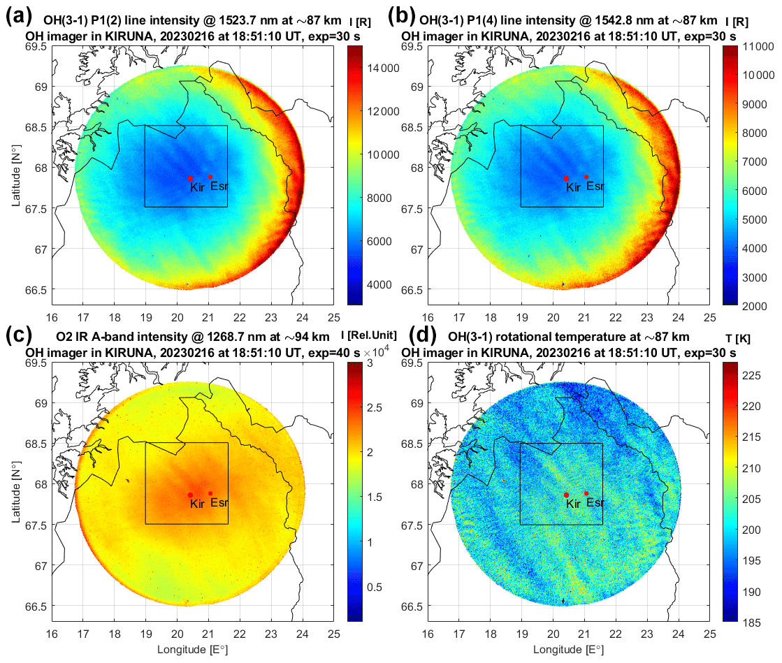
Figure 6 Maps of airglow intensities and temperature obtained from the OH imager on 16 February 2023. (a) Intensity in the rayleigh of the OH(3-1) P₁(2) line at 1523.7 nm. (b) Intensity in the rayleigh of the OH(3-1) P₁(4) line at 1542.8 nm. (c) Intensity in relative units of the O₂ IR A-band at 1268.7 nm. (d) OH(3-1) rotational temperature estimated using the brightness ratio of the two OH(3-1) emission lines (see text). The timestamp in all the maps corresponds to the time of the middle point of the current filter wheel cycle, which takes 2.75 min. The black squares show a zoom of the images, which is shown in Fig. 7.

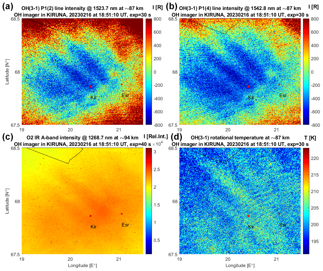
Figure 7 A zoom of the images shown in the black squares in Fig. 6, which focus on the small-scale wave structure of about 4–6 km wavelengths in (a) the P₁(2) map, (b) the P₁(4) map, (c) intensity in relative units of the O₂ IR A-band at 1268.7 nm, and (d) the temperature map. Residuals of the P₁(2) and P₁(4) intensities are shown after subtraction of the mean intensity values from these zoomed-in images.

The OH(3-1) daily mean rotational temperatures measured above Kiruna for the 2023 winter season (13 January–16 April) are illustrated by the black circles in Fig. 8. The OH(3-1) temperature values are within the range of 178–224 K. The average daily winter temperature for this particular period is equal to 203 ± 10 K. For comparison, Aura MLS temperatures close to the Kiruna location (less than 675 km away) are indicated by the red circles. There is good agreement between these time series, with a small average temperature difference of 1.9 ± 6.9 K. The temperature behavior agrees well with the general seasonal temperature behavior in the winter mesopause, with a maximum in the period of December–February followed by a rapid temperature decrease in March–April (e.g., Perminov et al., 2018). Kim et al. (2017) have analyzed mesopause temperatures from OH airglow measurements with a Fourier-transform spectrometer (FTS) for the winter periods of 2003–2014 in Kiruna. The authors have found variations in the winter mesopause temperature above Kiruna in the range of 180–230 K. This temperature range agrees well with the OH(3-1) temperature values presented in Fig. 8. Cho et al. (2011) have studied OH and O₂ airglow temperatures for the winter periods of 2001–2007, measured with a spectral airglow temperature imager (SATI) instrument and a Michelson interferometer, at high northern latitudes at Resolute Bay and Esrange, respectively. Cho et al. (2011) have demonstrated that winter mesopause temperatures vary between 180 and 245 K, which again agrees well with the temperature range obtained by the OH imager. Sigernes et al. (2003) have studied daily mesospheric winter temperatures for more than 20 years of ground-based spectral measurements of the OH layer over Svalbard from 1980 to 2001. The authors have found the average daily winter temperature to be equal to 208 ± 15 K, with a maximum and minimum temperature of 257 and 168 K, respectively, emphasizing that the mesospheric temperature variations over Svalbard in winter are extremely high. The average daily winter OH(3-1) temperature that was estimated in the present study is close to the value found by Sigernes et al. (2003), taking into account the large temperature deviations of the average daily values found in both papers.

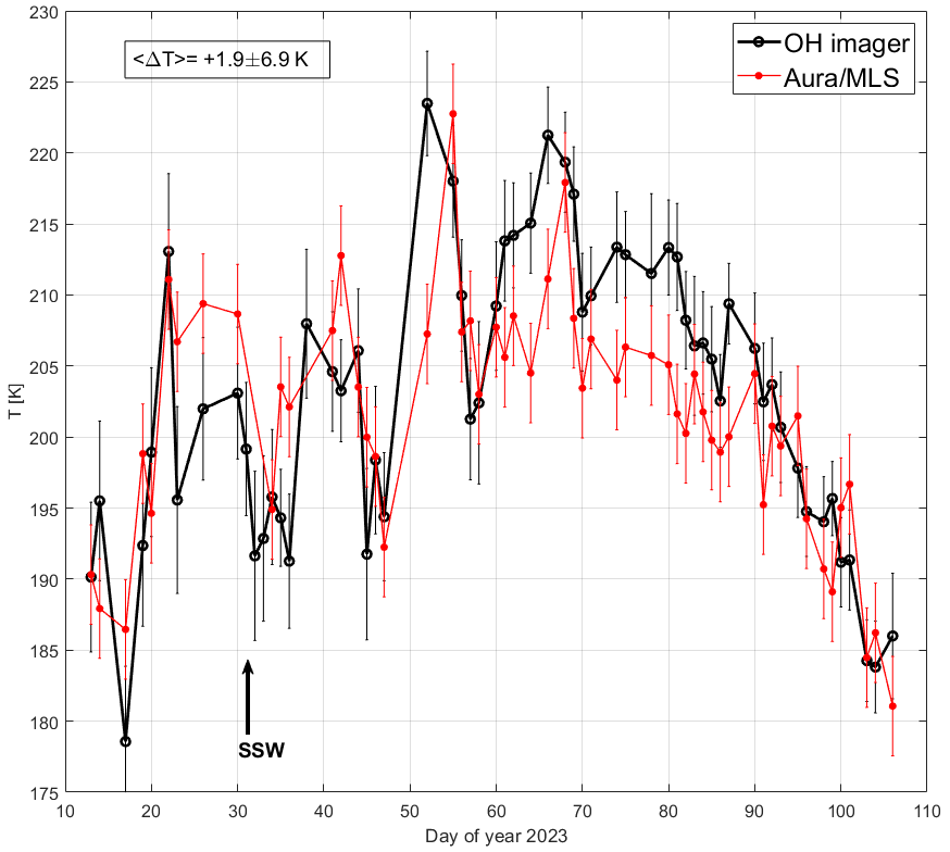
Figure 8 Daily mean OH(3-1) rotational temperature above Kiruna, at zenith, at ∼ 87 km for the 2023 winter season (black circles). Aura MLS instantaneous temperature measurements close to the Kiruna location at ∼ 86 km (red points). Error bars of the OH(3-1) temperature are 1 standard deviation for a particular night. Error bars of the Aura MLS temperature are equal to 3.5 K (see text). The onset of the sudden stratospheric warming is marked by the black arrow. The period considered is from 13 January to 16 April 2023.

It is interesting to discuss the following feature of the OH(3-1) temperature behavior: we observed two rather strong temperature enhancements on day 52 (21 February 2023) and on day 66 (7 March 2023). The 2023 sudden stratospheric warming (SSW) event started around 1 February 2023 (https://www.climate.gov/news-features/event-tracker/disrupted-polar-vortex-brings-sudden-stratospheric- warming-february, last access: 29 Febraury 2024). SSWs are accompanied by both cooling and warming of the mesopause region: cooling is observed at the time of an SSW onset or a few days later, while warming is observed with a delay of about 20–25 d (Cho et al., 2004; Shepherd et al., 2014). Sometimes several mesopause warmings (wavy oscillations) can be generated after an SSW onset (see Fig. 1b, f in Shepherd et al., 2014). This is exactly what was observed in the OH(3-1) temperature behavior: first, there was an OH(3-1) temperature decrease between days 32 and 36 (close to the 2023 SSW onset), and then the two strong temperature maxima occurred on days 52 and 66, i.e., about 20 and 34 d after the 2023 SSW onset. A detailed link of the OH(3-1) temperature above Kiruna to SSW events will be investigated in future papers.

The two emission layers (OH and O₂) are varied in space and time, making different height distances between these layers. This complicates an analysis dealing with the vertical propagation of gravity waves. At the same time, if the same wave package with the same horizontal wavelength, observed phase velocity and propagation direction is observed in both the OH and O₂ layers, one can assume that the same gravity wave was propagating in both the horizontal and vertical domains. According to the general theory of gravity waves (e.g., Gossard and Hook, 1975), a gravity wave propagates at an angle relative to the vertical, with tilted phase lines. This should result in an observed phase shift of the same gravity wave between the OH and O₂ layers. Once a phase shift and a horizontal wavelength are estimated from the OH and O₂ maps, one can calculate the vertical wavelength using the following relation:

$$\begin{array}{}\text{(6)}& {\mathit{\lambda }}_z={\mathit{\lambda }}_x/\tan \left(\mathit{\alpha }\right),\end{array}$$

where λ_z and λ_x are the vertical and horizontal wavelengths of a gravity wave and α is the angle between wave phase lines and the vertical. Furthermore, if the buoyancy frequency N is a known quantity or is estimated using lidar or satellite temperature profiles, one can deduce the intrinsic frequency ω of a gravity wave from the following relation:

$$\begin{array}{}\text{(7)}& \mathit{\omega }=\pm N\cdot \cos \left(\mathit{\alpha }\right).\end{array}$$

By substituting known values of ω, N and λ_x into the dispersion relation for gravity waves, one can estimate the vertical wavelength again, thus verifying the first estimation of the vertical wavelength. Note that this method is valid for a limited number of gravity waves with vertical wavelengths less than the height distance between the two layers (about 7 km).

Another simple method to estimate the vertical wavelength of a gravity wave is based on the assumption that the height difference D between the two layers is a known quantity (Fagundes et al., 1995; Schmidt et al., 2018). If a horizontal phase shift Δφ of a given wave package between both layers is estimated, then one can calculate its vertical wavelength λ_z using the following relation:

$$\begin{array}{}\text{(8)}& {\mathit{\lambda }}_z=D\cdot \mathrm{2}\mathit{\pi }/\mathrm{\Delta }\mathit{\phi }.\end{array}$$

We will use both approaches to estimate vertical wavelengths of gravity waves propagating through the OH and O₂ layers in a future paper, which will be supported by model studies of gravity waves propagating through the whole atmosphere up to the mesopause level (Dalin et al., 2015, 2016).

6 Conclusions

A novel infrared imager (OH imager) began operating in November 2022 in Kiruna (northern Sweden), aimed at studying nightglow emissions coming from the hydroxyl and molecular oxygen layers in the mesopause region. The OH imager registers selected emission lines (1523 and 1542 nm) in the OH(3-1) band to obtain emission intensity and temperature maps at around 87 km altitude. In addition, the imager records infrared emissions coming from the O₂ IR A-band airglow at 1269 nm in order to obtain O₂ emission intensity maps at a slightly higher altitude of ∼ 94 km. This technique allows for the tracing of gravity-wave disturbances in both the horizontal and vertical domains in the mesopause region. The lee location of the OH imager favors studies of mountain waves and their probable influence on the mesopause temperature and dynamics.

Temperature maps demonstrate the ability of the OH imager to resolve small-scale (4–8 km), small-amplitude (4–6 K) gravity waves as well as medium-scale gravity waves with horizontal wavelengths of 20–40 km and temperature amplitudes of 7–10 K. Such medium-scale waves have propagated through both the OH and O₂ layers.

The comparison between the OH imager and collocated Esrange lidar shows good agreement between OH(3-1) and Esrange lidar temperature measurements on individual nights (within 3 K) and on an average basis (−0.2 ± 1.6 K). The comparison between the OH imager and Aura MLS radiometer demonstrates no systematic temperature bias between these instruments and a small average temperature difference of 2.8 ± 7.8 K, which is likely caused by the variable state of the mesopause temperature over the spatial scales of their different observational volumes.

OH(3-1) daily mean rotational temperatures measured above Kiruna for the 2023 winter season (January–April) demonstrate typical seasonal variations, with a maximum in February and a rapid temperature decrease in April in the winter polar mesopause. The OH(3-1) temperature values are within the range of 178–224 K, which agrees well with other high-latitude temperature measurements in the winter mesopause. The average daily winter temperature for the period considered is 203 ± 10 K.