the Creative Commons Attribution 4.0 License.
the Creative Commons Attribution 4.0 License.
 | 25 Mar 2024
CALOTRITON: a convective boundary layer height estimation algorithm from ultra-high-frequency (UHF) wind profiler data
Alban Philibert
Marie Lothon
Julien Amestoy
Pierre-Yves Meslin
Solène Derrien
Yannick Bezombes
Bernard Campistron
Fabienne Lohou
Antoine Vial
Guylaine Canut-Rocafort
Joachim Reuder
Jennifer K. Brooke
Long time series of observations of atmospheric dynamics and composition are collected at the French Pyrenean Platform for Observation of the Atmosphere (P2OA). Planetary boundary layer depth is a key variable of the climate system, but it remains difficult to estimate and analyse statistically. In order to obtain reliable estimates of the convective boundary layer height (Zi) and to allow long-term series analyses, a new restitution algorithm, named CALOTRITON, has been developed. It is based on the observations of an ultra-high-frequency (UHF) radar wind profiler (RWP) from P2OA with the help of other instruments for evaluation. Estimates of Zi are based on the principle that the top of the convective boundary layer is associated with both a marked inversion and a decrease in turbulence. Those two criteria are respectively manifested by larger RWP reflectivity and smaller vertical-velocity Doppler spectral width. With this in mind, we introduce a new UHF-deduced dimensionless parameter which weighs the air refractive index structure coefficient with the inverse of vertical velocity standard deviation to the power of x. We then search for the most appropriate local maxima of this parameter for Zi estimates with defined criteria and constraints such as temporal continuity. Given that Zi should correspond to fair-weather cloud base height, we use ceilometer data to optimize our choice of the power x and find that x=3 provides the best comparisons. The estimates of Zi by CALOTRITON are evaluated using different Zi estimates deduced from radiosounding according to different definitions. The comparison shows excellent results with a regression coefficient of up to 0.96 and a root-mean-square error of 71 m, which is close to the vertical resolution of the UHF RWP of 75 m, when conditions are optimal. In more complex situations, that is when the atmospheric vertical structure is itself particularly ambiguous, secondary retrievals allow us to identify potential thermal internal boundary layers or residual layers and help to qualify the Zi estimations. Frequent estimate errors are observed nevertheless; for example, when Zi is below the UHF RWP first reliable gate or when the boundary layer begins its transition to a stable nocturnal boundary layer.
- Article
(7778 KB) - Full-text XML
- BibTeX
- EndNote


1.1 Instrumental techniques for convective boundary layer retrieval
The convective boundary layer (CBL) depth (Zi) is a key variable in the climate system for its role in modulating energy, water, and trace species exchange at the interface between the surface and free atmosphere. For this reason, it has significant applications in the fields of air quality, numerical weather predictions, climate models, and applied sectors such as renewable energy production. There are challenges in understanding the role of the convective boundary layer over heterogeneous surfaces; in complex terrains, coastal areas, and polar regions; and for surface–atmospheric exchange, transport, and mesoscale circulation, all of which require a comprehensive estimate of the CBL depth. Nevertheless, it remains difficult to accurately and exhaustively quantify it in the real world in terms of both the spatial and temporal variability due to its complexity.
Instrumental techniques for Zi retrieval are numerous and have led to an abundance of literature. Kotthaus et al. (2023) propose a recent overview of the CBL top detection techniques with an exhaustive description of their capabilities and limitations. Here we summarize the most relevant techniques applicable to this study.
There are several ways to identify Zi based on its characteristic atmospheric processes, which can be used to define different observational techniques. They can be classified into three main approaches based on the (i) thermodynamical processes, (ii) turbulent processes, and (iii) tracers. Figure 1 schematizes those various definitions through the vertical profiles of key variables.
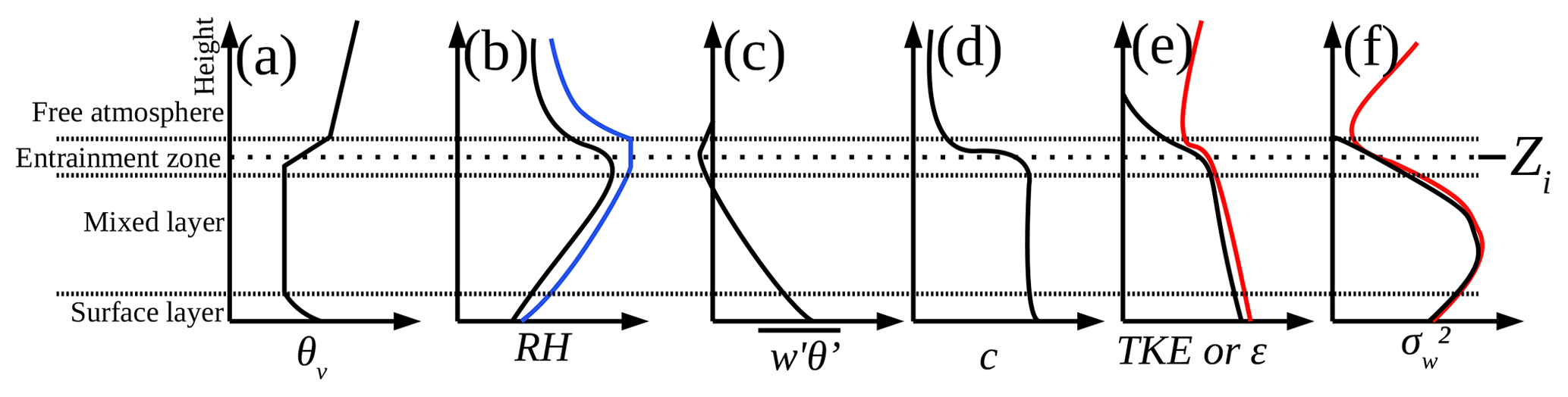
Figure 1Idealized CBL profiles (black line) of the (a) potential temperature, (b) relative humidity (blue line indicates the situation in the presence of clouds), (c) buoyancy flux, (d) scalar concentration, (e) turbulence kinetic energy (TKE) or TKE dissipation rate (ε), and (f) vertical velocity variance (red line indicates the situation in the presence of external forcing).
The thermodynamical approach considers Zi to be the height from the surface at which the summital inversion occurs, characterized by strong gradients of temperature and moisture (Fig. 1a, b). Several instrumental methods estimate Zi based on this approach, such as
-
the detection of the gradients of either the potential temperature, relative humidity (RH), or water vapour mixing ratio (e.g. Hennemuth and Lammert, 2006);
-
the detection of the maximum of relative humidity (Couvreux et al., 2016);
-
the so-called parcel method, which considers the potential temperature (or virtual potential temperature) at the surface θs and searches for the height above the surface where θ = θs (Holzworth, 1964) or θ = θs + δθ, where δθ is a small positive variation in surface potential temperature (Seibert et al., 2000).
In situ measurements from radiosounding, aircraft, or remotely piloted aircraft systems (RPASs) can be used based on this approach. Remote sensing provides an indirect measure of thermodynamical variables such as microwave radiometers, Raman lidar, or differential absorption lidar. Indirectly related to this approach, ultra-high-frequency (UHF) radar wind profilers (RWPs) in L-band are also appropriate devices to detect the CBL summital inversion, which is associated with a significant increase in reflectivity (White, 1993; Angevine et al., 1994).
Approaches based on turbulent processes consider Zi to be the height from the surface where turbulence intensity starts to strongly decrease (Fig. 1e). This height is coupled with the minimum (and negative) buoyancy flux (Deardorff, 1972) and a decrease in vertical velocity variance (Stull, 1988), turbulence kinetic energy (TKE), or TKE dissipation rate (ε). Both buoyancy flux and vertical velocity variance reach zero above Zi in textbook cases (unforced conditions and clear air). However, in cases of external forcing such as clouds, wind shear, or advection, a local minimum can be observed on each profile (see the red line in Fig. 1e, f). Doppler lidar and UHF RWPs give information on the turbulence intensity (Frehlich et al., 2006; Jacoby-Koaly et al., 2002, respectively). The variance of the Doppler velocity (Lothon et al., 2006) or the turbulence kinetic energy dissipation rate (e.g. Frehlich et al., 2006) can be used to detect the CBL top based on a threshold. Note that studies based on numerical weather predictions models often use TKE as a reference for Zi determination (Couvreux et al., 2016), whereas studies based on large eddy simulation often consider the minimum of the buoyancy flux (e.g. Pino et al., 2006). This makes those turbulence-based approaches very relevant for model evaluation.
The tracer-based approach considers Zi to be the height from the surface where strong discontinuity is observed in scalar concentration profiles (Fig. 1d) such as aerosol or gas concentration. Optical remote sensing such as lidar and ceilometers measure the optical backscatter coefficient from which aerosol concentration can be inferred (see Kotthaus et al., 2023, for an exhaustive list). Wavelet methods are typically used to detect the top of the more loaded CBL (e.g. Haeffelin et al., 2012), where the aerosol concentration abruptly falls from the CBL to the free troposphere (see e.g. Davis et al., 2000, for the use of the Haar-wavelet-based method). The mixing ratio maximum gradient method described above could also be considered a scalar concentration approach.
Some approaches use the synergy of instruments or methods. The bulk Richardson method (Hanna, 1969), with a threshold on the gradient Richardson number, is a combination of the wind gradient and the potential temperature gradient. The complementarity of instruments is widely used for Zi estimations. For example, Min et al. (2020) or Turner and Lohnert (2021) use the association of a microwave radiometer with a ceilometer or Raman lidar respectively. Since they are based on different definitions, all the methods discussed potentially result in slightly different estimates of Zi (Caicedo et al., 2017), especially when the observed CBL is not a simple idealized case.
In this study, we revisit the methodology of estimating Zi from UHF RWP measurements and propose a new complementary algorithm. The advantage of RWPs relative to other remote sensing devices is their ability to measure in all weather types and not be limited by cloud types and the amount thereof, precipitation, or clear-sky conditions. Their height coverage limitation is predominately related due to water vapour content. One known weakness is their sensitivity to bird echoes, which typically occur in the nighttime during bird migration events, particularly in spring and autumn. It is usually not a significant issue during daytime convection.
1.2 Motivations and main objectives
The multi-instrumented site of the ACTRIS-Fr1 infrastructure, the Pyrenean Platform for Observation of the Atmosphere (P2OA – Lothon et al., 2024), gathers a comprehensive set of instruments for the monitoring of the atmosphere, with a subselection of instrumentation located at the Centre de Recherches Atmosphériques (CRA), Campistrous, in south-west France, close to the Pyrenees mountain ridge. Among them, a UHF RWP purchased by the LAERO3 laboratory has continuously measured the boundary layer since 2010. Retrieving the CBL height from this instrument from this multi-year time series allows for a statistical study of the dynamical processes in this mountainous region. These processes include the influence of plain–mountain circulations and thermally driven winds, the interaction between mountain waves and the boundary layer, and the impact of mesoscale subsidence related to orographic convection. This unique dataset enables us to make statistical analyses and climatologies, with applications in air quality, weather forecasting, and climate studies.
An existing technique, partly based on Angevine et al. (1994), was used for this specific radar to estimate Zi (Jacoby-Koaly et al., 2002). Angevine et al. (1994) base the estimate of Zi on the absolute maximum of the air refractive index structure coefficient (), which, however, does not always correspond to the current CBL top but can correspond to the residual inversion above. To address this, Jacoby-Koaly et al. (2002) attempted to retrieve the local maximum of that could be the most appropriate estimate of Zi by using temporal continuity and other criteria. This is also the approach of Collaud Coen et al. (2014). Note that reaches local maxima where temperature and humidity show not only large vertical gradients, but also large wind gradients and turbulence (which induces fluctuations in the air refractive index). This technique provides very satisfying results on a case-by-case investigation for fair-weather convective conditions without the complex vertical structure of the atmosphere (Heo et al., 2003; Jacoby-Koaly, 2000). However, statistical studies of the time series based on this technique may not be possible without significant errors. One obvious limitation, for example, is that it often catches the top of the residual layer in the early morning rather than the top of the shallower developing CBL top. The temporal continuity criterion does not solve this issue. Attributing Zi to the top of the residual layer during the morning transition potentially leads to large errors. This can also occur in late afternoon, when this method will likely attribute Zi to the top of the pre-residual layer (Nilsson et al., 2016b) and then residual layer, while true Zi may decay with the decreasing surface heat flux and decaying turbulence layer (Grimsdell and Angevine, 2002; Lothon et al., 2014). It can also catch upper inversions, which are not directly connected to the mixed layer. Also note that residual layers are not always a local phenomenon but may be advected (Angevine, 2000). In the presence of clouds at different levels, the difficulties increase due to more complexity, with greater stratification of the atmosphere and in cloud turbulence (Grimsdell and Angevine, 1998; Angevine, 2000; Collaud Coen et al., 2014; Duncan et al., 2022).
Several other techniques are based on the same principle of the existence of a local maximum of reflectivity. For example, Liu et al. (2019) use local maxima of normalized signal-to-noise ratio (SNR); Compton et al. (2013) use the covariance wavelet transform to detect the large step in SNR associated with Zi; and Molod et al. (2015) use a simple algorithm with the use of SNR, based on the determination of the “emergence time”, and corresponding height and temporal continuity, based on backscatter standard deviation. All of them, however, encounter the same difficulties mentioned above, to a greater or lesser extent. Molod et al. (2015) used this technique to retrieve long series of Zi from a network of profilers, but the departure from in situ estimates based on the bulk Richardson number shows that although simple and significantly robust, the proposed algorithm still cannot handle the high complexity of the low troposphere. Collaud Coen et al. (2014) developed a climatology of the CBL height based on multiple remote sensing instruments and validated the dataset against radiosoundings. They found that their estimates from the RWP were more dispersed due to false attributions, revealing the difficulty of this approach when dealing with the various encountered conditions.
One way to improve this method is to also consider the decrease in turbulence at the top of the convective layer (see Fig. 1e, f) combined with the association to a local maximum of (Heo et al., 2003) or SNR (Bianco and Wilczak, 2002; Bianco et al., 2008). Heo et al. (2003) assume that the zero buoyancy flux is reached where the vertical velocity standard deviation is null. They search for this height and then select the nearest local maximum of . With the same basic assumption, Bianco and Wilczak (2002) and Bianco et al. (2008) use the fuzzy logic method to determine the height which corresponds to the combination of radar variables. Those techniques definitely improve the CBL depth estimates relatively to the more standard approaches.
In this study, we use this same fundamental assumption and combination to improve the initial method used for the LAERO UHF RWP radar in order to develop a new algorithm to address a broader range of atmospheric conditions, including the complex vertical structure of the atmosphere, cloudy situations, and multilayered lower troposphere.
We present the experimental data used in Sect. 2, and we describe the Zi-retrieval algorithm (CALOTRITON) and discuss the choice of configuration parameters in Sect. 3. Illustrative examples are given in Sect. 4, and a comparison of the CALOTRITON UHF-based Zi estimates to in situ measurements is presented in Sect. 5. A conclusive discussion is presented in Sect. 6.
2.1 Datasets
In this study, we consider the data of the LAERO UHF RWP at P2OA-CRA from 2015 to 2022 to develop the new CALOTRITON algorithm. This time period is shorter than the whole available time series for the sake of data process homogeneity. The year 2018 is more intensively used for the primary development of the algorithm. We also use sensible heat flux measurements from a sonic anemometer installed at 30 m on the P2OA-CRA 60 m instrumented tower and relative humidity measurements made at 2 m.
To optimize CALOTRITON parameters, we compare Zi estimates with cloud base heights (Sect. 3.3) measured by a CT25k ceilometer from Centre National de Recherche Météorologique (CNRM) present from December 2016 to December 2019 at P2OA-CRA.
The algorithm results are then validated (see Sect. 5) by comparison to in situ profiles made using a radiosonde or remotely piloted aircraft system (RPAS) during two intensive field campaigns; (i) BLLAST (Boundary-Layer Late Afternoon and Sunset Turbulence; Lothon et al., 2014), which took place at P2OA-CRA, and (ii) LIAISE (Land surface Interactions with the Atmosphere over the Iberian Semi-arid Environment; Boone et al., 2021), which took place in north-east Spain, close to Lleida. The latter enables us to test CALOTRITON in a meteorological and geographical context other than that of the long-term observational record of P2OA-CRA and thus generalize its applicability and use. For both measurement campaigns, the CNRM UHF RWP is used in addition to the LAERO UHF RWP, which also enables testing the algorithm on a different UHF RWP.
Table 1 summarizes the contexts of RWP measurements used and corresponding time periods, the location of RWPs, the complementary instrumentation used, and their role in this study. The corresponding datasets are listed and referenced in the “Data availability” section at the end of the article, with more precision on the specific periods for each instrument.
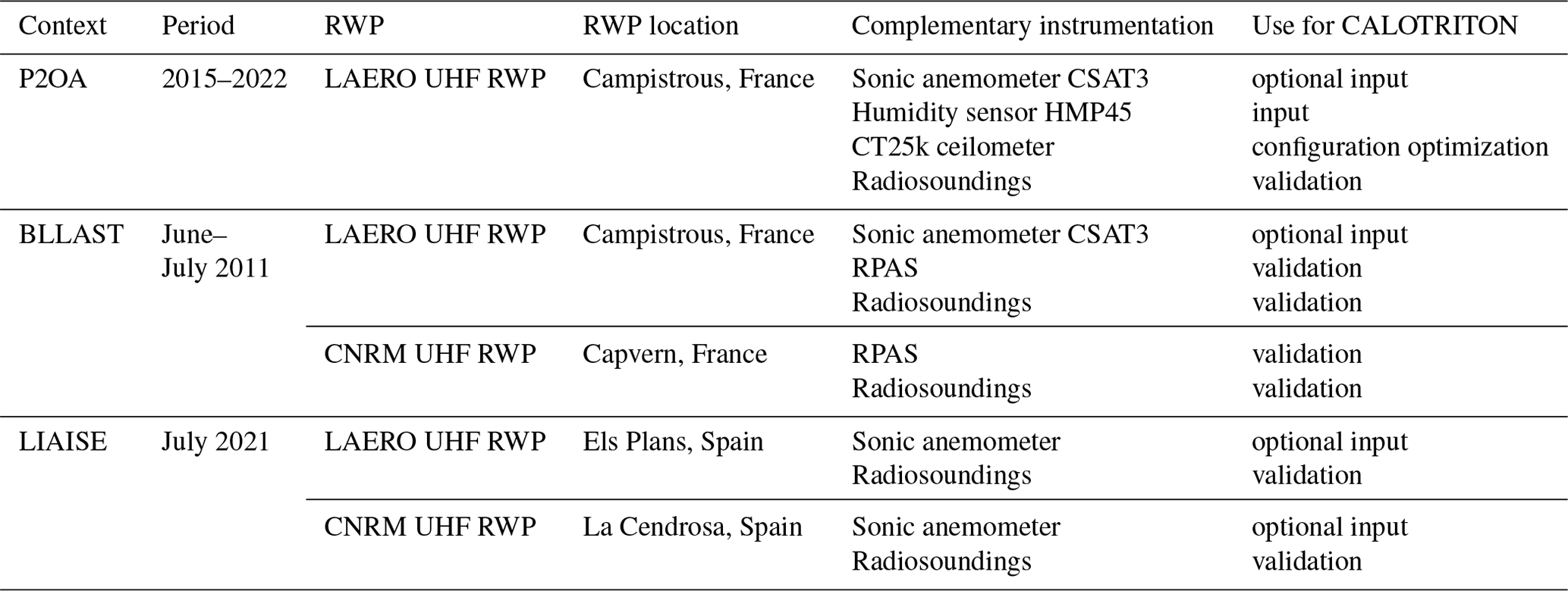
The sensible heat flux is calculated using 30 min duration samples with EddyPro software, based on the eddy correlation technique. The UHF RWP instruments and data process are detailed in the following section.
2.2 UHF radar wind profiler technical characteristics and data process
The LAERO UHF RWP is a 1.274 GHz wind profiler with five beams, four oblique beams, and one vertical beam. Its main characteristics are listed in Table 2 (for more details, see Jacoby-Koaly, 2000). It alternates between two modes: a “low mode” with a pulse width of 500 ns corresponding to a range resolution of 75 m and a “high mode” with the pulse width of 2.5 µs corresponding to a range resolution of 150 m and a slightly better height coverage. For our use here, we only consider the low mode. The maximum height for this mode is usually around 3000 m a.g.l. but may be only 500 or 1000 m in winter, when dry anticyclonic conditions occur. It can reach 7 or 9 km within deeper clouds and rain. The first gate is at 75 m but with a poor confidence index. We consider the 225 m gate to be the first gate with very good confidence. The CNRM UHF RWP mainly presents the same characteristics but with the first level with a good confidence index at 300 m.
Table 2Main characteristics of the Laboratoire d’Aérologie's ultra-high-frequency radar wind profiler (LAERO UHF RWP; https://p2oa.aeris-data.fr/sedoo_instruments/profileur-de-vent-uhf/, last access: 22 March 2024).
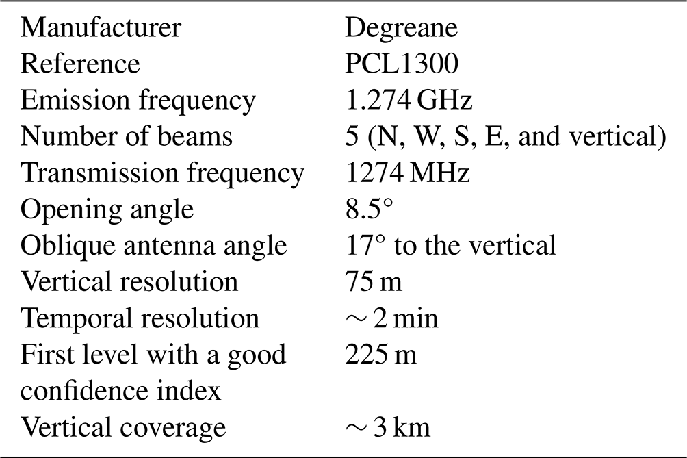
The three components of the wind are deduced from the Doppler radial velocity of the five beams every 75 m and every 2 min. The first main critical step is to select the meteorological peak from the Doppler spectrum. We use a process developed at the LAERO laboratory, which optimizes the meteorological peak selection and data coverage relative to the manufacturer processing. During this phase, an automatic quality control is done, eliminating Doppler spectral erroneous peaks before the wind component calculation. The second step is typical of the velocity volume processing technique (Wadteufel and Corbin, 1979), which computes the three wind components from the radial velocity with a minimum least-squares error. The air refractive index structure coefficient is deduced from the reflectivity as a function of the received power (Doviak and Zrnic, 1993). The vertical velocity variance is obtained from the Doppler spectral half-width of the backscattered signal on the vertical beam and gives and allows for the estimation of TKE dissipation rate ε (Cohn and Angevine, 2000; Jacoby-Koaly et al., 2002). Hereafter, is the median air refractive index structure coefficient over the five beams and depends on altitude and time. ε is the median TKE dissipation rate over the five beams. σw is deduced from the vertical antenna and corrected for the effect of the horizontal wind within the antenna aperture (Jacoby-Koaly et al., 2002). All those variables are calculated at 2 min time intervals.
3.1 CALOTRITON specific objectives
The new Zi-retrieval algorithm (CALOTRITON) was developed with five main objectives and constraints in mind:
-
to restrict the Zi estimate to the convective boundary layer by only considering daytime conditions and excluding precipitation periods;
-
to respect the temporal continuity of Zi growth and to follow it as finely as possible in time in order to describe the smallest convective scales (5 to 30 min; Stull, 1988), as Zi should start close to the ground early in the day;
-
to manage complex cases, as in the presence of clouds or thermal internal boundary layer (TIBL) or when cold air advection in the lower layers can create a new convective boundary layer such as in the case of slope wind (Kossmann et al., 1998) or sea breeze (Durand et al., 1989);
-
to take into account abrupt CBL growth, which occurs in the presence of a residual neutral layer above Zi, when the current CBL potential temperature gets to reach the residual neutral layer potential temperature (Blay-Carreras et al., 2014);
-
to use limited instrumental synergy in order to apply it in other sites (or measurement campaigns) equipped with a UHF RWP and not to depend on the availability of an advanced instrument suite to establish the Zi estimate.
3.2 CALOTRITON operation
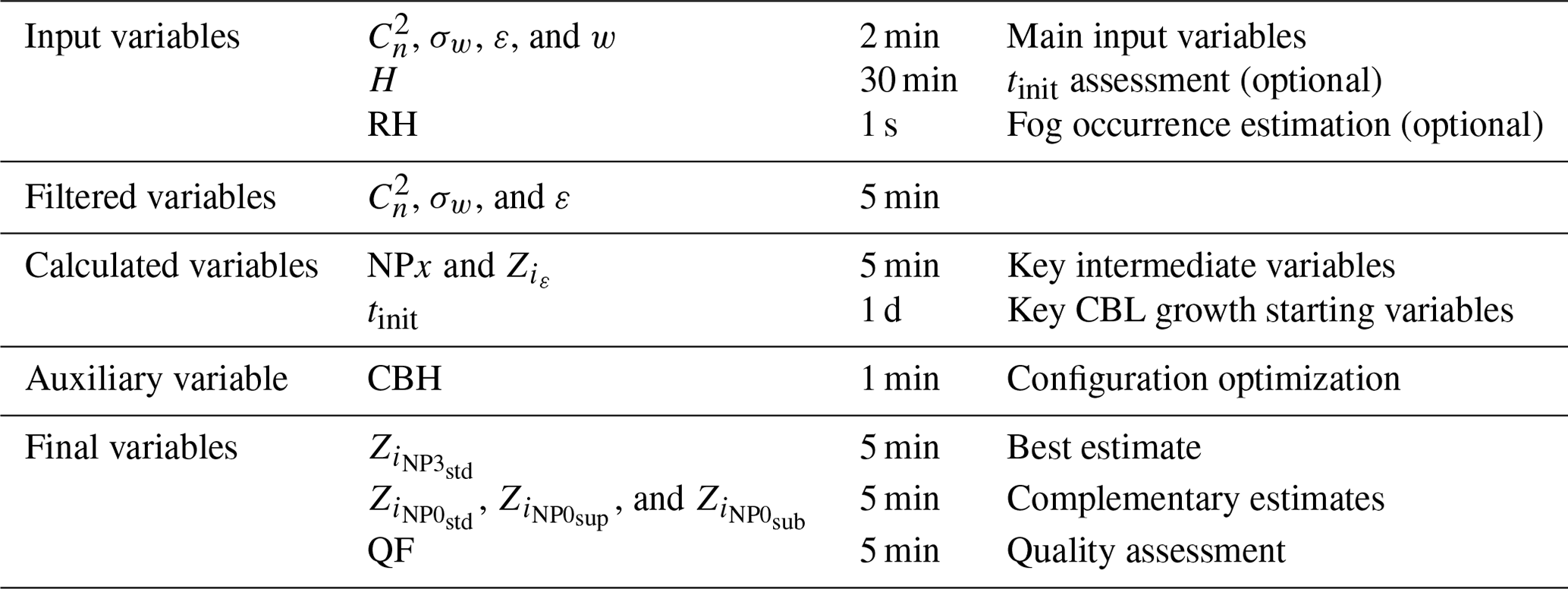
Figure 2 presents a scheme of the CALOTRITON algorithm, which is described in this section, and Table 3 recapitulates the variables used at the different steps of CALOTRITON with the corresponding timescales.
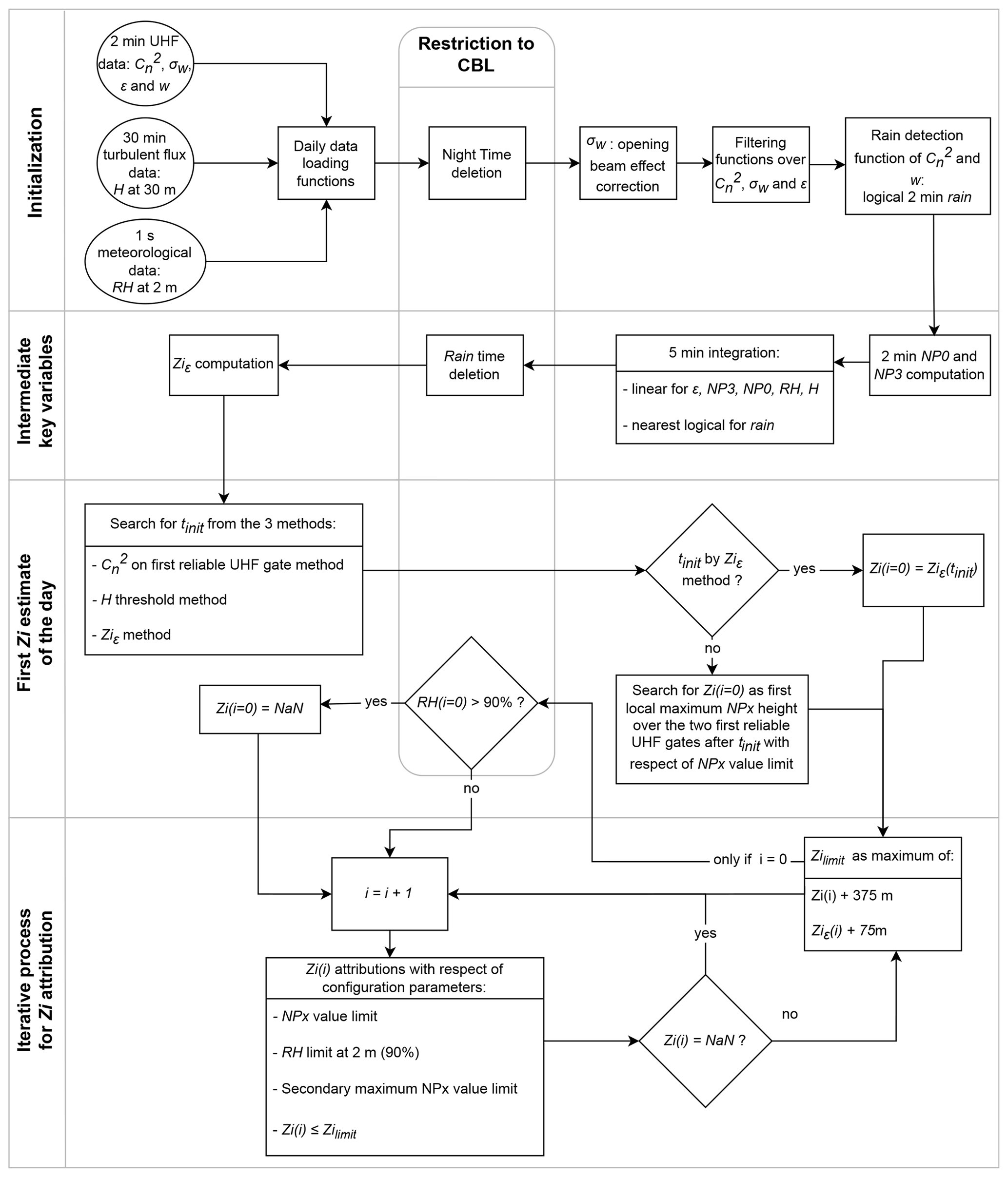
Table 3Variables used in CALOTRITON at the different steps of the algorithm and their time intervals.
3.2.1 Restriction to CBL conditions
First, we consider UHF RWP data only above 225 m a.g.l. and below 3000 m a.g.l. The height of 225 m is the first gate where data are always of high quality. Only daytime data are selected to estimate Zi from the UHF RWP. For this, sunrise and sunset times are retrieved as a function of date, altitude, latitude, and longitude. Precipitation periods (including virga) are excluded by a function based on empirical thresholds on and Doppler vertical velocity (w). Any profile which meets > 10−14 m and m s−1 over five consecutive levels is removed, including all profiles occurring 15 min before and after. We do not assign Zi in the case of fogs, notably due to the limitation of the UHF RWP below 225 m a.g.l. It was found at the P2OA site that relative humidity at 2 m larger than 90 % was associated with fog occurrence as confirmed by ceilometer measurements (not shown). We therefore take this as a criterion for fog occurrence and remove corresponding periods from the further analysis.
3.2.2 Data averaging
In order to disregard non-meteorological disturbances (e.g. birds) affecting the UHF RWP signal, , σw, and ε data are filtered by complementary sliding median filters:
-
and ε – a median over 6 min (three data points), none over the height in order to keep the original UHF RWP vertical resolution of 75 m;
-
σw – a median over 8 min (four data points) and a median over 225 m (three points) because of a more pronounced spatiotemporal variability in these data (see Figs. 4d, 6d, 8d), using coarser filters for σw to compensate for the fact that and ε are already integrated over the five beams.
If a larger integrated time is chosen, the corresponding median time filter should be adjusted and applied to , ε, and σw.
3.2.3 Definition of intermediate key variables
As the reflectivity maximum does not always correspond to Zi, especially in the case of a cloudy sky, we suggest using a new dimensionless variable which takes into account both the increase in reflectivity at the summital inversion and the decrease in turbulence; the variable NPx (Eq. 1) weighs by σw to the power of x and allows for a better account of a large value of associated with a small value of σw. Dimensionless NPx is obtained by averaging values of and up to 3000 m for each profile (overlines in Eq. 1):
Dimensionless NPx is computed with the filtered data discussed previously (Sect. 3.2.2) and is linearly integrated over a 5 min time step to describe the smallest characteristic convective scale. The choice of x is discussed in Sect. 3.3.2. As an example, Figs. 4d and 6d discussed later show cross sections of NP3 in a simple and complex case respectively. Note that this approach is based on the same main assumption as in the methods proposed by Heo et al. (2003) and Bianco and Wilczak (2002), who also combined the need for an increase in reflectivity and a decrease in turbulence.
We also consider another variable purely defined by the level of turbulence; variable is the height above the surface at which the TKE dissipation rate ε falls below m2 s−3. This technique was previously used by Couvreux et al. (2016) and Nilsson et al. (2016a). It thus represents a rough estimate of the depth of significant turbulence. Height is computed on filtered and integrated ε data (5 min as NPx). In order to consider only the that would respect a certain temporal continuity, a sliding median filter over 15 min (three points) is applied to .
Variable NPx is the core variable of CALOTRITON, but will help us with documenting the associated turbulence and optimize the selection of the most appropriate local maximum of NPx as an estimate of Zi (we hereafter call this selection “Zi attribution”).
3.2.4 Determination of the first Zi estimate of the day
In a typical CBL development, Zi starts close to the ground, below the UHF RWP detection limits (225 m), and grows until it reaches a plateau in the early afternoon (Stull, 1988). It is therefore necessary to wait for some time (called tinit) before Zi can be detected by the UHF RWP. We found that the sensible heat flux, which governs the evolution of Zi, remains very low (lower than a few tens of W) at least until 1.5 h after sunrise (not shown). Therefore, tinit is not defined before 1.5 h has passed after sunrise.
Several methods are used to determine tinit. The first is based on at the first reliable UHF RWP gate (225 m a.g.l.) and considers tinit to be the time when the 30 min sliding median exceeds its daily mean value. That way, it is investigated when an increase in becomes significant and may correspond to Zi. The second method is based on the measured sensible heat flux (H) and considers tinit when H exceeds the significant threshold of 50 W m−2. In that case, tinit is taken as the earliest time over those two. The first assigned Zi of the day (Zi(i=0)) can only be established at a local maximum of the vertical profile of NPx located at one of the two first reliable levels of the UHF RWP and occurring after tinit.
Sometimes, a thin layer is mixed by dynamical turbulence before sunrise, e.g. in the presence of a low-level jet. In order to take those situations into account, we allow the attribution of the first Zi at the height of if the latter corresponds exactly to the height of the NPx maximum of the profile independently of tinit and provided that this attribution is always done 1.5 h after sunrise.
This initialization process is somehow similar to Molod et al. (2015), who called this time the “emergence time” and determined it based on the same principle; i.e. they also consider a first good-confidence gate and look for the first determinable Zi at this level but in a different way.
3.2.5 Iterative process for Zi attribution
Once the initial Zi is found, the search for subsequent Zi is done by temporal iteration on the most significant local maximum of NPx that is located within a vertical growth limit of 375 m since its last effective attribution. Residual layers or clouds above Zi can potentially return a higher signal contribution to NPx than Zi itself and might be misinterpreted if located within the 375 m growth limit. To take this into account, the algorithm allows for attributions to local secondary maxima of NPx below the first maximum value if the value of the corresponding NPx is at least 90 % of the first maximum value of NPx before 10:00 UTC and 50 % after. These empirical values are discussed in Sect. 3.3.2 and named relative thresholds of the secondary maximum of NPx. Finally, a minimum value of NPx is required for attribution and fixed to the mean profile value of NPx in order to take into account a certain significance. Sometimes, strong growth of Zi can occur and exceed the imposed limit (375 m). This motivated us to use in order to consider up to which level significant turbulence is found. If at i time is higher than the last effective attribution plus the growth limit, then Zi(i) can be searched up to + dz (where dz=75 m).
3.3 Algorithm parameter choice
3.3.1 Parameter optimization
All the parameters presented above were obtained empirically by subjectively judging the quality of the attributions of Zi for about 100 d in 2018 at P2OA-CRA. In order to verify their quality in a more objective way and possibly to adjust some parameters, we compared the estimates of Zi with the lowest cloud base height (CBH) measured by the CT25k ceilometer within a 5 min interval of each attribution. This comparison is based on data from December 2016 to December 2019. When comparing the two configurations with the distributions shown in Fig. 3, one would favour the configuration which leads to fewer attributions above cloud base and lower values of ε at Zi.
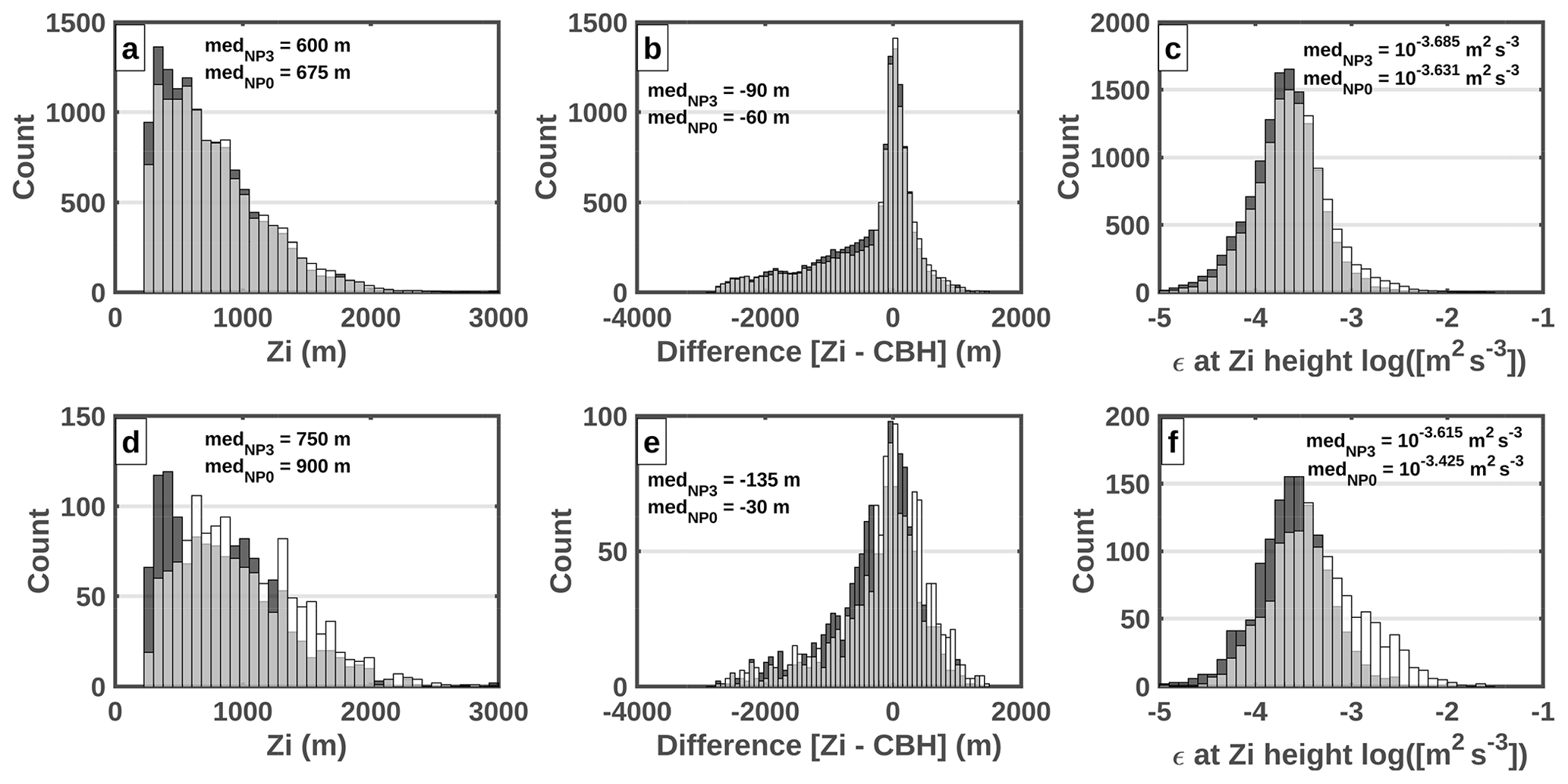
Figure 3Histograms showing the differences between the distributions of (white bar) and (black bar) in the presence of clouds measured by the CT25k ceilometer from December 2016 to December 2019: (a) Zi distribution, (b) distribution of difference between Zi and cloud base height, and (c) ε-value distribution at Zi height. Panels (d) to (f) are respectively the same as panels (a) to (c) but considering only attributions which present more than 225 m difference between and . For the distributions of and , the median values are indicated by medNP3 and medNP0 respectively.
Table 4List of the best parameters for CALOTRITON configuration.
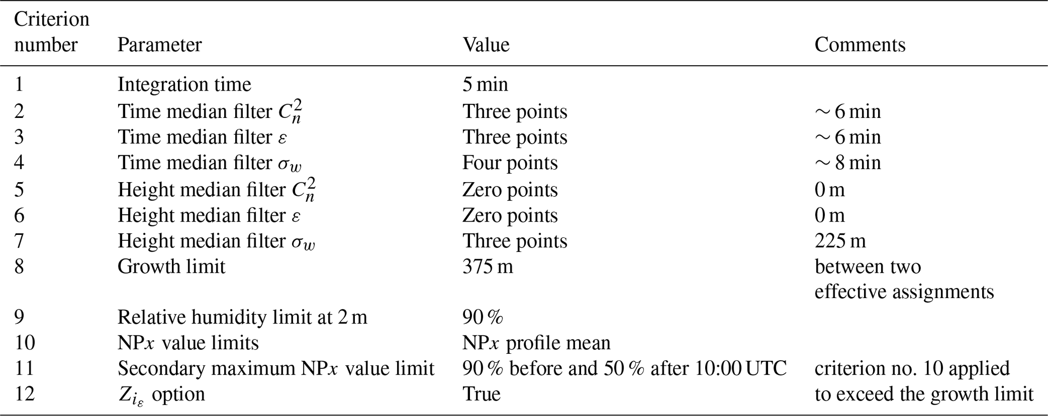
Figure 3 shows an example of the results of this comparison for Zi estimates based on either NP3 or NP0, with the use of the optimal parameters listed in Table 4. Figure 3a shows the distribution of the set of Zi attributions for the different values of NPx (x=0 and x=3) and indicates more attributions by NP3, especially for Zi<700 m. Figure 3b shows the distribution of the differences between Zi and CBH. It can be seen that there are slightly more attributions above the cloud base when using NP0. Figure 3c presents the distribution of all ε values at Zi height and shows that NP3 attributions tend to get lower ε values at Zi height. The fact that NP3 attributions of Zi are more often lower than NP0 attributions and associated with lower ε values is a sign of better quality attributions. When clouds are present, the difference between Zi estimates based on NP3 and NP0 is on average twice as large as in clear-sky cases due to the complexity of the atmosphere in cloudy conditions. Thus, the observed differences between Zi attributions based on NP3 and NP0 give an indication of the CBL complexity. Figure 3d–f present the same figure as the top panels (Fig. 3a–c) but only considering the attributions by NP3 and NP0 when they differ by more than 225 m from each other. This represents only 10 % of the total attributions. The same conclusions as previously stated can be drawn even more clearly here. We therefore confirm that NP3 statistically gives better results.
3.3.2 Tested parameters and optimum set
In this way, the set of NPx values for x=1 to x=5 was compared two by two with the configuration presented in Table 4. It was noted that attributions were potentially better for x=3 than x=0, 1, or 2. However, no significant trend was noticed for x≥3. We limit ourselves to x=3 in order to keep the attributions predominantly based on . In this section, only a few results of our search for the best parameters by attribution distribution analysis are presented. All are based on NP3. The largest differences appeared between whether or not we considered a limit on relative humidity. Not setting a limit allows for about 4 % more attributions in clear-sky conditions and 40 % more in the presence of clouds. Among those 40 %, half of them correspond to cloud base heights below 225 m, which is the first level of the UHF RWP. Considering the limit on relative humidity, 13 % of all attributions in the presence of clouds take place 225 m above the cloud base compared to 22 % without a limit. This limit, therefore, both avoids attributions in the presence of clouds whose base is below the UHF RWP lower limit and reduces the number of attributions above the cloud base by half.
The methods for the search for tinit were tested. Using solely the maximum technique leads to almost no difference in Zi attributions, but, additionally, using the technique based on sensible heat flux leads to 3 % more attributions.
Other values related to the growth limit were also tested. It was noticed that a limit of 300 m with the last effective attribution potentially allows for better quality attributions to be obtained but leads to a reduction of 3 % in the attributions compared to a limit of 375 m. Empirically, it was found that 300 m was not sufficient to properly track the evolution of Zi compared to 375 m. On the other hand, a 450 m growth threshold did not improve the results statistically. Although it leads to an increase in the total number of attributions by 3 %, all additional attributions under cloudy skies were above the cloud base. This is the reason we finally chose 375 m as the optimal growth threshold.
Other important parameters are the values selected for the relative thresholds of secondary maximum NPx on which attributions are possible. Not setting a limit leads to an increase of 40 % in attributions above CBH + 225 m, which is associated with higher ε values and thus less appropriate. Thresholds of 50 % and 90 % were tested over the whole day, and it was found that the threshold of 50 % led to more attributions over residual layers than the threshold of 90 %, especially in the morning. In contrast, a threshold of 90 % leads to more attributions inside the CBL, especially in the afternoon. This is why thresholds of 90 % before 10:00 UTC and of 50 % afterwards were chosen. A threshold of 75 % for the whole day was also tested but provided poorer results.
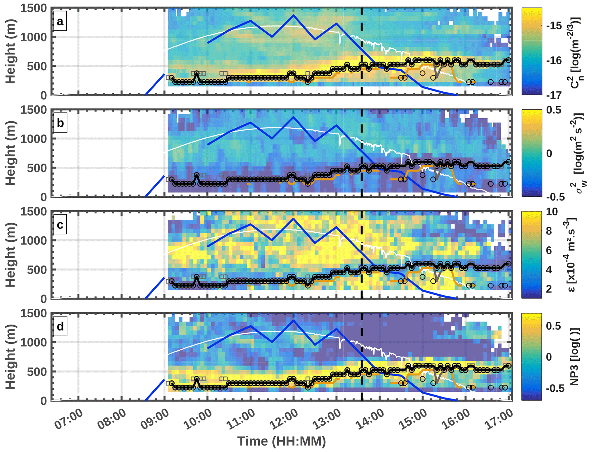
Figure 4UHF RWP observations for 27 October 2021 at P2OA-CRA during clear-sky conditions: (a) filtered in log scale, (b) filtered in log scale, (c) filtered and integrated ε in log scale, and (d) integrated NP3 in log scale. For all panels, Zi estimates are as described in Sect. 3.2.2 and 3.3.3 – (orange line), (grey line), (grey squares), (black line), and (black circles) – and based on the same ordinate axis (but with different units), i.e. downward shortwave radiation (W m−2) (white line) and sensible heat flux (dW m−2) (thick blue line). The vertical dashed line corresponds to the time of the discussed radiosounding.
3.3.3 Final assignment and flags
As we have seen previously, the difference between NP0 and NP3 attributions with the parameter set as described in Table 4 gives useful and complementary information about the complexity of the lower troposphere. This is why we perform the following four estimates of Zi:
-
is estimated with the standard configuration for NP3 as described in Table 4, which is considered to be the best set of attributions.
-
is estimated with the standard configuration for NP0 as described in Table 4.
-
is estimated from NP0 as described in Table 4 but without applying criteria nos. 9, 10, and 11. With this configuration, the 375 m growth limit (no. 8) is applied between the Zi searched for and the already allocated maximum Zi. There is also no tinit restriction after sunrise. This configuration allows for the search for levels higher than the estimates made with a standard configuration, which may correspond to the top of a residual layer or to Zi if the standard configuration assigns it to a TIBL top.
-
is estimated from NP3 as described in Table 4 but without applying criterion no. 11. With this configuration, the NPx profile mean of the criterion no. 10 is replaced by the median, which gives lower values most of the time, mainly because of high values of . This configuration allows us to search for levels lower than the estimates made with a standard configuration, which may correspond to a TIBL top or to Zi if the standard configuration assigns it to a residual layer top.
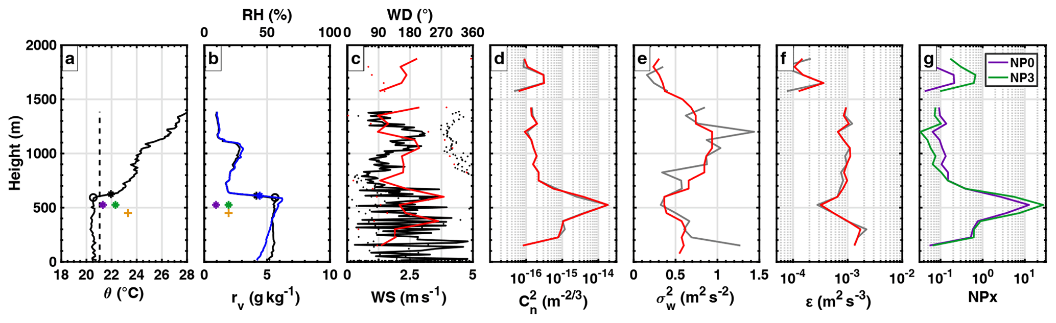
Figure 5Profiles measured by radiosondes and UHF RWP at P2OA-CRA on 27 October 2021 at 13:35 UTC. (a) Potential temperature (solid black line), surface potential temperature +0.25 °C (dashed black line), Zi from the in situ subjective method (black circle), Zi from the in situ potential temperature gradient method (black asterisk), (purple “×”), (purple “+”), (green “×”), (green “+”), and (orange “+”). (b) Mixing ratio (black line) and relative humidity (blue line), Zi from the in situ mixing ratio gradient method (black asterisk), Zi from the in situ relative humidity gradient method (blue asterisk); purple, green, and orange crosses denote the same values as described in panel (a). (c) Wind speed (solid line) and wind direction (dotted line) from the radiosonde (black) and UHF RWP (red). (d) Air refractive index structure coefficient from UHF RWP with raw data (grey line) and filtered data as described in Sect. 3.2.2 (red line). (e) Vertical velocity variance from UHF RWP with the same colour scheme as in panel (d). (f) TKE dissipation rate from UHF RWP with the same colour scheme as in panel (d). (g) NP0 (purple line) and NP3 (green line).
Our best proposed estimate is for the reasons explained earlier. However, the four estimates embed the large complexity that is often observed in the lower troposphere.
In order to qualify this complexity and to facilitate the correct use of the four estimates, a quality flag QF is defined as follows:
-
When QF = 1, all attributions are equal. It indicates very good confidence in the assignment quality and a textbook case.
-
When QF = 2, only , , and are equal. It indicates good confidence in the assignment quality and the likely presence of a residual layer above Zi located at . It also indicates that the Zi estimate does not match the height of the maximum.
-
When QF = 3, only , , and are equal. It indicates medium confidence in the assignment quality and the likely presence of a TIBL located at .
-
When QF = 4, only and are in exact agreement. It indicates medium confidence in the assignment quality and the likely presence of both a TIBL and a residual layer located at and respectively.
-
When Q = 5, there is no agreement between the four attributions of heights. This indicates poor confidence in the assignment quality and a highly complex case.
Other flags could be produced in order to more thoroughly document the meaning of those various estimates. They could, for example, qualify the temporal continuity of (i.e. the occurrence of abrupt changes) or the consistency of with .
In this section, we present three study cases to illustrate the capability of CALOTRITON and the improvements of Zi retrieval relatively to a more standard approach:
-
a reference simple clear-sky case (27 October 2021 at P2OA),
-
a complex cloudy-sky case (15 March 2018 at P2OA),
-
a complex multiple-layering clear-sky case (27 July 2021 during the LIAISE field experiment).
4.1 Clear-sky case at P2OA
Figure 4 shows the height–time section of four UHF-based variables defined earlier: the air refractive index structure coefficient (Fig. 4a), the air vertical velocity variance (Fig. 4b), the turbulence kinetic energy (TKE) dissipation rate ε (Fig. 4c), and the new combined parameter NP3 (Fig. 4d).
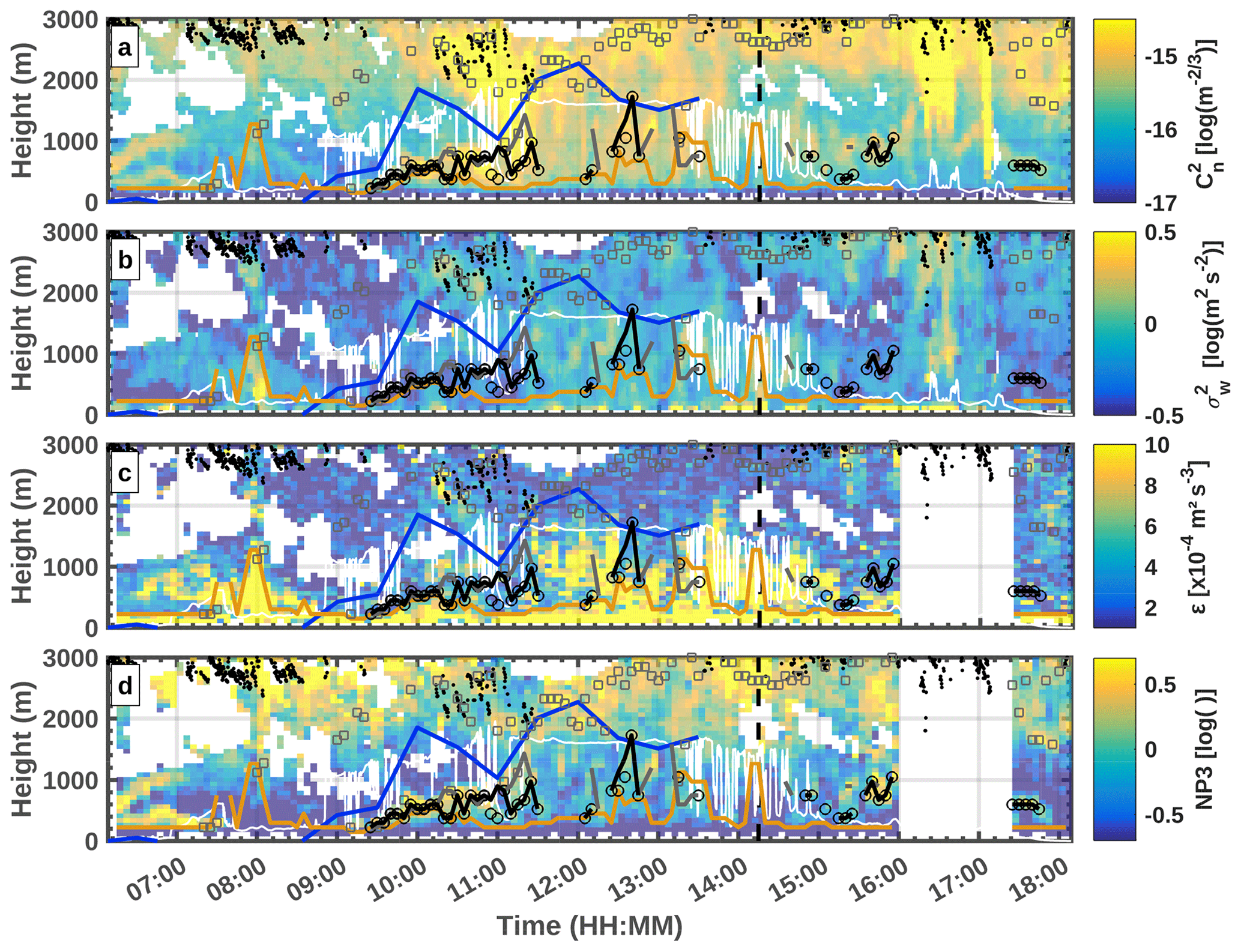
Figure 6LAERO UHF RWP observations for 15 March 2018 at P2OA-CRA with the same description as Fig. 4 and cloud base height measured by the CT25k ceilometer (black dots).
The downward shortwave radiation (white line) and the sensible heat flux (blue line) are overlaid on all panels. The shortwave radiation shows that this day was mainly clear with only a few thin and occasional cirrus clouds in the afternoon. Sensible heat flux shows a typical diurnal cycle. Also overlaid are different estimates of Zi defined in the previous section (, , , and ) and the intermediate variable . We note for this case very large consistency between the four different estimates . That means whatever the method, standard or more sophisticated, taking account of turbulence intensity or not, they all agree for the Zi estimation for the CBL growth and simply match the absolute maximum reflectivity for most of the time.
In order to make the correspondence between the UHF RWP and the thermodynamical profiles, Fig. 5 compares in situ measurements of thermodynamical variables measured by radiosondes with the UHF RWP measured variables at 13:35 UTC on this same clear day of 27 October 2021.
The comparison shows that the absolute maximum reflectivity corresponds well to the CBL top, characterized by a strong gradient of the potential temperature and mixing ratio (Fig. 5a and b). It also shows that (Fig. 5e) and ε (Fig. 5f) are small at this height, leading to a local minimum. On “ideal” clear days without external forcing, we would typically not observe significant turbulence above Zi (Fig. 1e). In this case, forcing is small with weak wind, but the wind shears still generate significant turbulence (Fig. 4c). In a subjective way, we estimate Zi at about 550 m from this radiosonde, where a strong potential temperature gradient is observed, which is associated with a strong humidity gradient (mixing ratio and relative humidity). This height is in good agreement with all the estimates made by CALOTRITON at that time and with the simplest standard estimate of Zi made by RWP. This case is a typical clear-sky case with QF =1 for most of the day (Fig. 4). Height consequently has a good confidence index, except around 15:30 UTC, where is slightly lower than . Note in Fig. 4 that remains equal to or below those estimates and especially decreases in the late afternoon with a strong decay of the surface flux. This is one typical late afternoon transition scenario, as described in Grimsdell and Angevine (2002) and Lothon et al. (2014). Value also interestingly decays during the same phase, thus defining a potential pre-residual layer situated between (or ) and (or ). The pre-residual layer is defined when the surface heat flux is not strong enough anymore to keep the mixing up to the midday summital inversion and falls between the thinning turbulence layer and the residual inversion (Nilsson et al., 2016b; Lothon et al., 2024). The different estimates made in CALOTRITON can thus help identify interfaces and layers in the complex afternoon transition phase. Standard and simple methods do not enable us to describe this subtle and still poorly understood complexity.
4.2 Complex cloudy case at P2OA
Figure 6 gives another example of UHF RWP measurements on 15 March 2018, this time with a marked external forcing, identified by a cloudy sky and high wind speed in the upper layer. For this figure, the cloud base height measured with the ceilometer is added and also revealed by the downward shortwave radiation.
In this complex case, the maximum of remains constant for most of the day between 2000 and 3000 m, related to the clouds and associated hydrometeors rather than to the top of the CBL. This makes high in this nearby cloud layer. Between 10:00 and 11:30 UTC, this maximum of is competitive with the local maximum below, which is what we can interpret as the top of the growing CBL and which is better detected with NP3. Between 16:00 and 17:20 UTC, the reflectivity field shows the presence of virga (verified by observations of the weather radars of Météo-France). In cases where droplet size is close to the RWP wavelength, this induces a strong reflectivity (and ) on the entirety of the profiles. For this more complex case, , , and are consistent only until 11:00 UTC. After this time, and are higher than and , suggesting that the latter may be assigned to the top of a TIBL. After 11:30 UTC, the assignments based on NP3 become more discontinuous due to the limit of NPx values (NPx profile mean). This discontinuity indicates an increased uncertainty in the attributions. Value is then systematically located above the others, suggesting that may potentially identify the top of a TIBL. However, we believe that these attributions are correct as they are located at the height where the strongest wind shear is observed. After 15:00 UTC, Fig. 6 shows more discontinuity on attributions, demonstrating a CBL complexity with small incoming shortwave radiation, no positive sensible heat flux, and the occurrence of precipitation mentioned above.
In order to better interpret this complex day, Fig. 7 compares in situ measurements of thermodynamical variables with the UHF RWP variables at 14:15 UTC on that same day.
In a subjective way, Zi can be estimated at 1500 m from this radiosounding (Fig. 7a), the height where the atmosphere starts to be stable (positive θ gradient), which is also associated with a strong discontinuity in the mixing ratio profile. This height corresponds well to . However, the absolute maximums of (Fig. 7d) and (indicated in Fig. 7a) correspond to an inversion around 2500 m, identified by a strong potential temperature gradient. This actually corresponds to a cloud base (see the black dots in Fig. 6) which is decoupled from the CBL. Value is thus inappropriate here. There is no marked local maximum of at the height of Zi estimated from the in situ radiosonde, but σw (Fig. 7e) and ε (Fig. 7f) profiles have a well-marked local minimum, forming a marked local maximum on NP3.
This example illustrates the benefit of taking σw into account via NPx with x>0 in the attribution of Zi. It also shows the advantage of the various Zi estimates to identify different interfaces in the case of complex vertical structure. Of course, the large complexity of this case and the weak CBL encountered in some phases of the day due to clouds and precipitation make this issue still difficult to deal with.
4.3 Clear sky with multiple layering during LIAISE
The use of the LIAISE dataset (Boone et al., 2021) allows us to test the CALOTRITON algorithm with the same UHF RWP at a different location and in different meteorological conditions. During the LIAISE campaign, the LAERO UHF RWP was deployed from June 2021 to October 2021 in the semi-arid region of Lleida, Spain, at a distance of about 15 km from large areas of irrigated crops. Figure 8 illustrates the complexity that can be observed in clear-sky conditions in this region and tests the capability of CALOTRITON for CBL with multilayer conditions. The analyses of this rich dataset have only recently started, but the study by Jimenez et al. (2023) already testifies to this complexity.
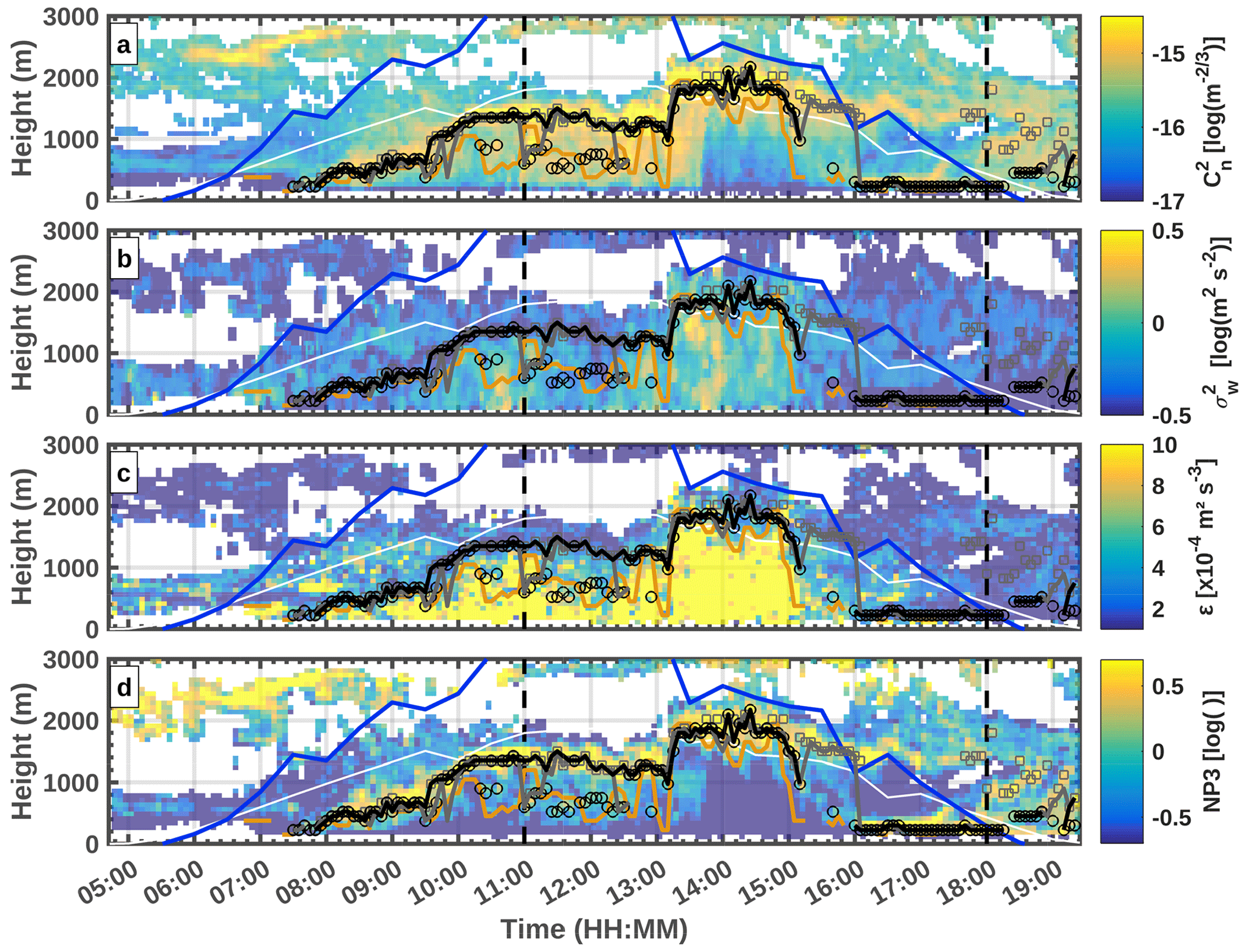
Figure 8LAERO UHF RWP observations for 27 July 2021 at Els Plans (Spain) during the LIAISE campaign with the same description as Fig. 4.
Early in the morning, an elevated local (actually absolute) maximum of is present between 2 and 3 km. This corresponds to a high inversion, potentially coming from a residual transported layer (shown later). An algorithm purely based on maximum would start the day with this erroneous Zi estimate. In CALOTRITON, the process of finding the first estimate of the day at the first possible gate enables us to avoid this situation. Most of the various Zi estimates agree until 09:30 UTC. Between 10:00 and 13:00 UTC, indicates the potential presence of a TIBL located below 1000 m, whilst at 11:00 UTC is at the level of at about 600 m. Firstly, note that the maximum discussed previously is still present at 11:00 UTC in Fig. 8a and corresponds to a large moisture and temperature inversion. It is not thin but associated with a large change in the water vapour mixing ratio.
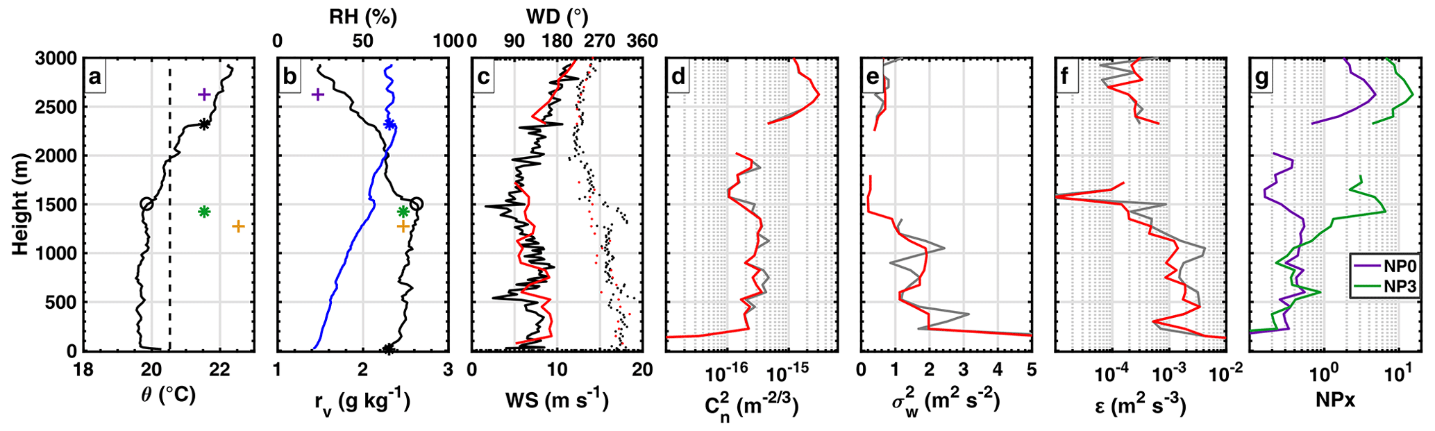
Figure 9 shows measurements from a radiosonde taken at this time.
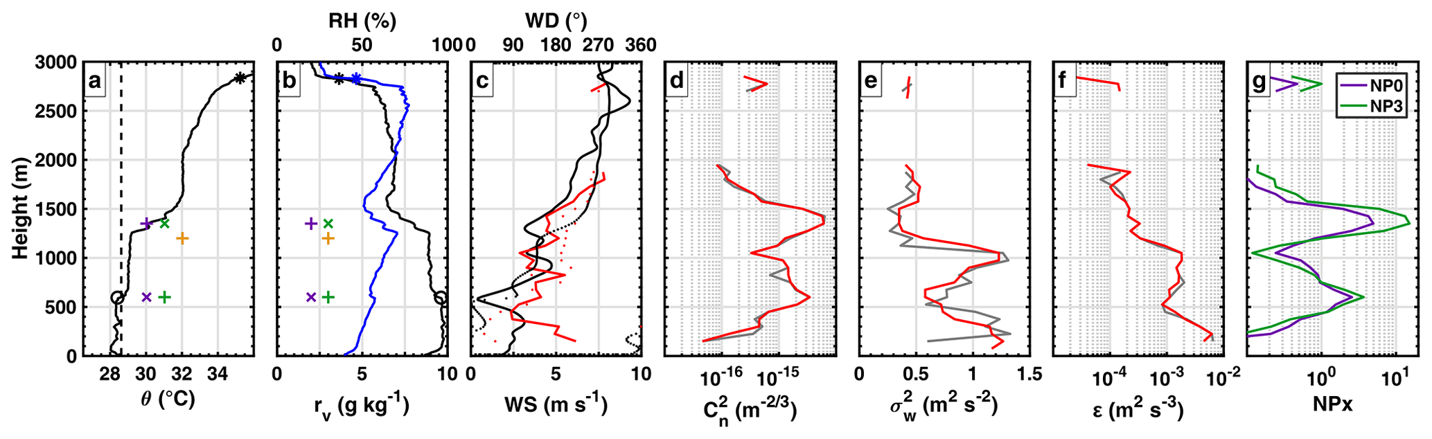
Figure 9Same as Fig. 5 but with profiles measured by radiosounding and LAERO UHF RWP at Els Plans (Spain) during the LIAISE campaign on 27 July 2021 at 11:00 UTC.
In the first 1500 m, we notice the presence of two superimposed layers with constant potential temperatures and mixing ratio (Fig. 9a and b) separated by a thermal inversion at 600 m. Strictly speaking, according to the definition of the thermodynamic approach, Zi should be located at the top of the first layer, since the surface over-adiabaticity (28 °C) theoretically does not allow a parcel of air to cross the inversion at 600 m (29 °C above). By a scalar concentration approach, Zi could also be attributed to 600 m where a discontinuity in the mixing ratio is indeed observed. The latter is, however, not considered to be very strong, and the fact that a constant (but slightly different) mixing ratio is observed above and up to 1300 m indicates mixing within this upper layer. An earlier sounding at 10:00 UTC (not shown here) reveals that the CBL was well mixed up to 1200 m a.g.l. on this day over this dry site. What is seen at 11:00 UTC in Fig. 9a and b is an intrusion of a nearby boundary layer likely advected into the region from the north-east, that is from the irrigated site, which has much thinner CBL. The cooler and moister air observed over the dry site in Fig. 8b up to 600 m is consistent with air coming from the irrigated area. In this case, that is over Els Plans, some turbulence structures may be able to overcome the 600 m high inversion and some others may not. We indeed find high turbulence values ( m2 s−3) up to 600 m. This turbulence contributes to the mixing of both layers and eroding the inversion. This is observed later in the soundings (not shown). Comparing the 11:00 UTC radiosonde profile with the UHF RWP estimates, defines Zi at 1300 m with the presence of a TIBL inside, whose top would be located at 600 m and detected by and .
In Fig. 8b–c, shortly after 13:00 UTC we notice a sudden increase in turbulence up to about 2000 m a.g.l. This may be due to another boundary layer advection as the wind direction (not shown) suddenly changes from ∼200 to ∼90° between ∼ 1000 and ∼ 2000 m. A break in the temporal continuity of NP3 local maxima is then observed, and the imposed growth limit does not allow us to follow this sudden evolution. The use of (1875 m at 13:15 UTC) allows for the attributions of and to follow this rapid change from 975 m at 13:10 UTC to 1800 m at 13:20 UTC. From 14:00 UTC onwards, a low-level marine breeze (<500 m) can be seen in Fig. 8a and b. This marine air is called “La Marinada” in this region (Jimenez et al., 2023) and is typical of the area. It is an entrance of marine air coming from the Mediterranean Sea, which is usually favoured by a continental heat low over northern Spain. Between 15:00 and 16:00 UTC, differences between and are observed, showing the high complexity of the atmosphere. After 16:00 UTC, all the attributions are made at 225 m on the first UHF RWP gate.
Figure 10 shows the data from a radiosonde launched at 18:00 UTC on the same day, where it can be seen that and are well established at the height of the maximum potential temperature and mixing ratio gradient. The observed breeze has therefore set up a new convective boundary layer.
At 19:00 UTC, the radiosonde data (not shown) indicate that Zi decreases below the first reliable RWP gate; CALOTRITON attributions are then erroneously overestimated by about 500 m a.g.l.
This example has shown a highly complex situation, which can occur even in clear-sky conditions. It exemplifies the complexity of automatically assigning Zi with radiosonde data or remote sensing when several boundary layers interact and lead to multilayering in the lower troposphere. It also illustrates how the different CALOTRITON attributions can help to identify CBL top, TIBL top, and the advection of internal boundary layers. The flag defined in Sect. 3.3.3 helps to identify the days when this kind of complex layering of the low troposphere may occur.
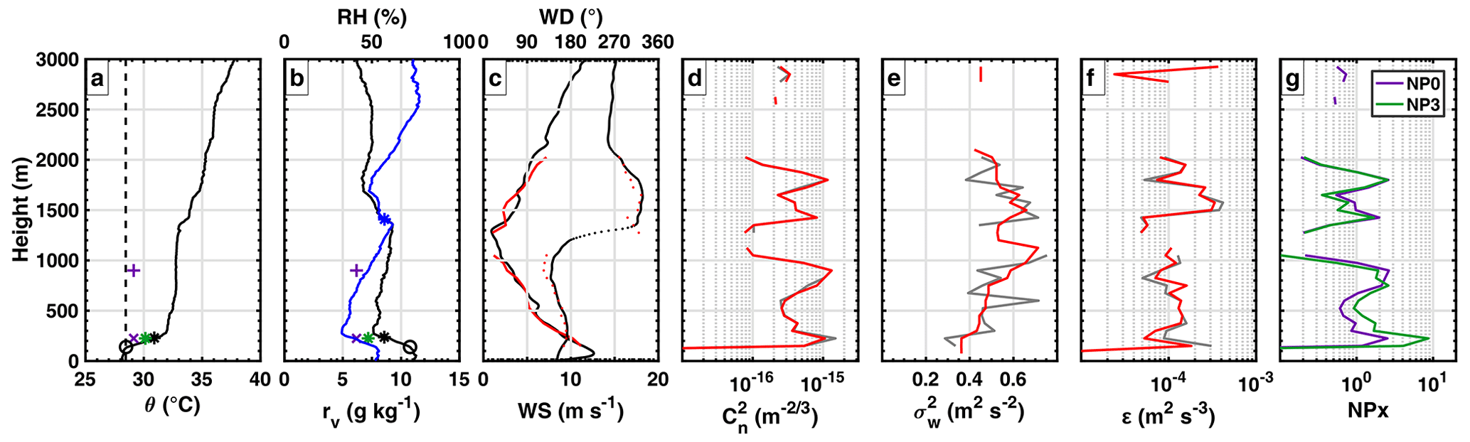
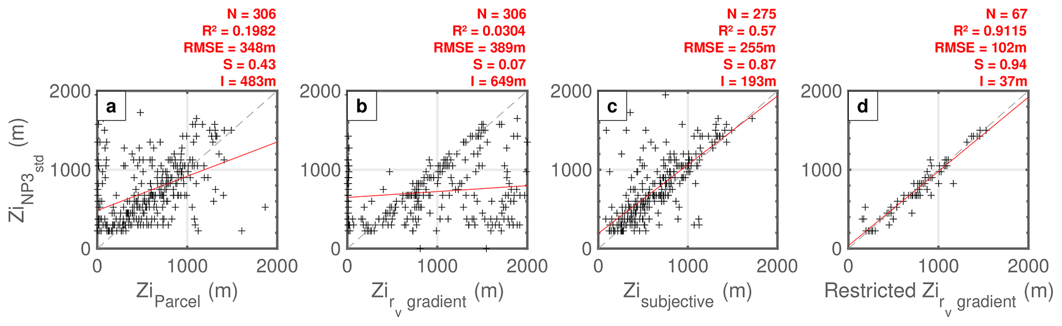
Figure 11Comparison between and (a) Zi from the in situ parcel method, (b) Zi from the in situ water vapour mixing ratio gradient method, (c) subjective Zi estimates, and (d) restricted Zi from the convergence of all the in situ-based estimates. In all panels, the dashed grey line represents the 1 : 1 slope, and the red line is the linear regression. The characteristics of the regression are indicated in red: the number of data points (N), the regression coefficient (R2), the root-mean-square error (RMSE), the regression slope (S), and the intercept (I).
The previous sections have shown that gives the best estimates of Zi. To validate this estimate, all CALOTRITON attributions were compared to the numerous radiosonde data made during the LIAISE and BLLAST field experiments near two UHF RWPs (Table 1). During BLLAST, the LAERO UHF RWP was at P2OA-CRA, and the CNRM UHF RWP was about 5 km to the south. RPAS (Reuder et al., 2016) profiles were made near the two sites, and radiosounding balloons were launched from both sites (Lothon et al., 2014; Legain et al., 2013), a few tens of metres from the RWPs. During LIAISE, the LAERO UHF RWP was installed on a dry area (Els Plans) and the CNRM UHF RWP was installed on an irrigated area (La Cendrosa) (see Sect. 4.3) about 15 km away (Boone et al., 2021). Radiosoundings were launched from the two sites as well, near the RWPs (also a few tens of metres away). A total of about 500 profiles are available for the evaluation of the CALOTRITON estimates. Median filters are applied over the vertical to the in situ data to match a vertical resolution of 10 m. Those numerous in situ profiles give the opportunity to evaluate and validate CALOTRITON and also give some insight into the results from automatic estimates from thermodynamic profiles.
In Fig. 11a–b, we compare with automatic in situ estimates based respectively on the parcel method (one of the most frequently used methods) and on the water vapour mixing ratio gradient method (as an example of the gradient method).
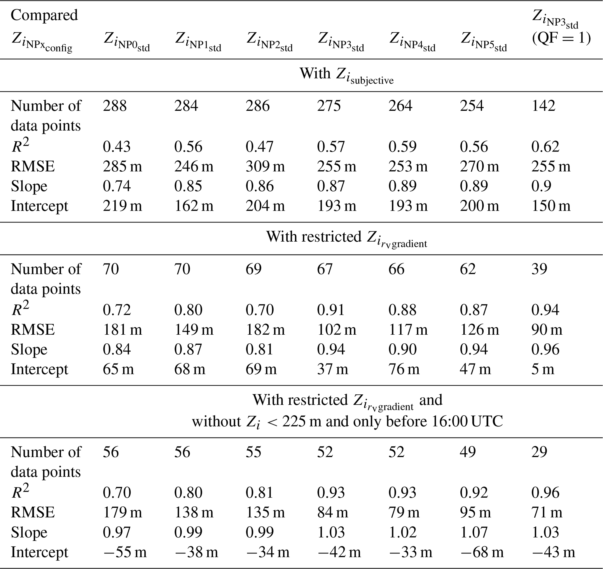
Table 5Summary of linear regression characteristics between Zi from CALOTRITON with NPx (x=0 to x=5) in standard configuration as described in Table 4 and Zi from the in situ subjective method; restricted Zi estimates based on the in situ mixing ratio gradient method, agreeing with other in situ-based estimates as described in the text; and the same Zi with further restrictions (no attributions below 225 m or after 16:00 UTC).
In the parcel method, a small amount δθ is added to the surface potential temperature (θs), and is defined as the height where above the surface (Seibert et al., 2000). Here we set δθ to 0.25 °C (Fig. 5a). A great disparity in points is observed, which is mainly explained by a poor estimation of in non-textbook cases. They are indeed either overestimated (example in Fig. 7a) or underestimated by the potential presence of TIBL (example in Fig. 9a). Value δθ may not always be appropriate, according to the actual super-adiabatism close to surface. In addition, a large number of small Zi estimates by the parcel method (<200 m) can be observed due to the observation of a positive potential temperature gradient in the very first metres of the profiles. Hennemuth and Lammert (2006) attribute this to evening transitions, but it may actually happen at any time (see Fig. 9a), for example, by the establishment of local breezes or other types of advection. It can also occur when the surface layer is not clear (showing fluctuations over the vertical) during the start and at the spot of the sounding. The parcel method may or may not be fair in those cases. The in situ radiosounding or RPAS profile are very local and instantaneous. Note that using the bulk Richardson method rather than the parcel method did not significantly change the result of this comparison (not shown). The bulk Richardson Zi estimates were actually slightly less relevant than the parcel method estimates with more frequent overestimation of Zi due to the attribution of Zi on upper inversions.
The in situ-based gradient methods assign Zi at the height of the strongest gradient of potential temperature, water vapour mixing ratio, or relative humidity below 3000 m. Figure 11b shows the comparison between and the water vapour mixing ratio gradient estimates. There is a large majority of cases where attributions based on the water vapour mixing ratio gradient method () are largely above . They mostly correspond to attributions to residual layers or upper inversion, as described by Hennemuth and Lammert (2006) and as seen in the previous examples (Figs. 7 and 9). Furthermore, a significant number of attributions by gradient methods are very low and correspond not only to the stable surface layer (around morning or evening transitions), but also to the fact that one can observe large fluctuations in the surface layer as seen in Fig. 7b. Similar results are found when considering the potential temperature or the relative humidity for the gradient method (not shown).
Figure 11a–b show that it remains difficult to qualify CALOTRITON estimates with the automatically determined estimates from in situ parcel or gradient methods. For this reason, a subjective method of assigning Zi from in situ thermodynamical profiles is helpful. We attempt to keep this method as objective as possible by assigning Zi at the height where we observe the first notable discontinuity in the mixing ratio profile associated with discontinuity in the potential temperature profile. The approach is similar to searching for the top of a conserved scalar tracer, and it should also correspond to the height where the entrainment zone starts (see Fig. 1d). Figure 11c shows the comparison of this subjective Zi with CALOTRITON estimates based on NP3std. We obtain a much better agreement between the attributions with a higher regression coefficient (R2=0.57), but some points still deviate from the trend, and this may be due to subjective misinterpretation as we have seen in the presence of TIBL, for example, or due to the failure of CALOTRITON estimates.
In order to disregard errors in the in situ estimates, we finally restrict the comparison of with in situ estimates to the cases where the standard deviation within the estimates from the various in situ methods is lower than 100 m. This way, we ensure consistency between those methods; that is, we keep the more “simple” or “textbook” situations. We also ensure objectivity. Figure 11d shows an excellent comparison between and Zi from the in situ mixing ratio gradient method in those conditions, with R2=0.91 and a root-mean-square error (RMSE) of 102 m. However, there are still a few points that deviate, which is mainly due to
-
late afternoon conditions, when the atmosphere starts to stabilize in the surface layer (In these cases, we are actually at the limit of the CBL definition);
-
attributions below the UHF RWP vertical detection limitation.
If we ignore in situ attributions below 225 m and at times later than 16:00 UTC, we obtain R2=0.93 and RMSE =84 m (which is close to the 75 m UHF RWP vertical resolution), which confirms the consistency of CALOTRITON estimates in those conditions.
Table 5 summarizes all the comparisons made between the UHF RWP CALOTRITON estimates (based on various orders of NPx in standard configuration as described in Table 4) and in situ estimates (based on the different methods). has slightly larger R2 and a lower RMSE when compared with the subjective in situ Zi estimates. However, generally, NP3std-based attributions are very similar to NP4std-based attributions and, moreover, lead to 4 % more attributions when compared to the subjective-method in situ estimates. This further supports the optimum choice of using to estimate Zi with CALOTRITON and the validity of those estimates. Finally, when we compare the attributions of NP3std with QF =1 with those of restricted , which both reflect a simple textbook case, the results are excellent with an R2 of more than 0.96 and an RMSE = 71 m, which is lower than the RWP vertical resolution (75 m).
Lothon (2023a)Saïd (2012)Lothon and Vial (2022)Garrouste (2011)Lothon (2023b)Lohou et al. (2023a, b)Lohou (2017)Price (2023a)Canut et al. (2022)Lothon (2018)Legain (2011)Price (2023b)Garrouste et al. (2022)Reuder and Jonassen (2017)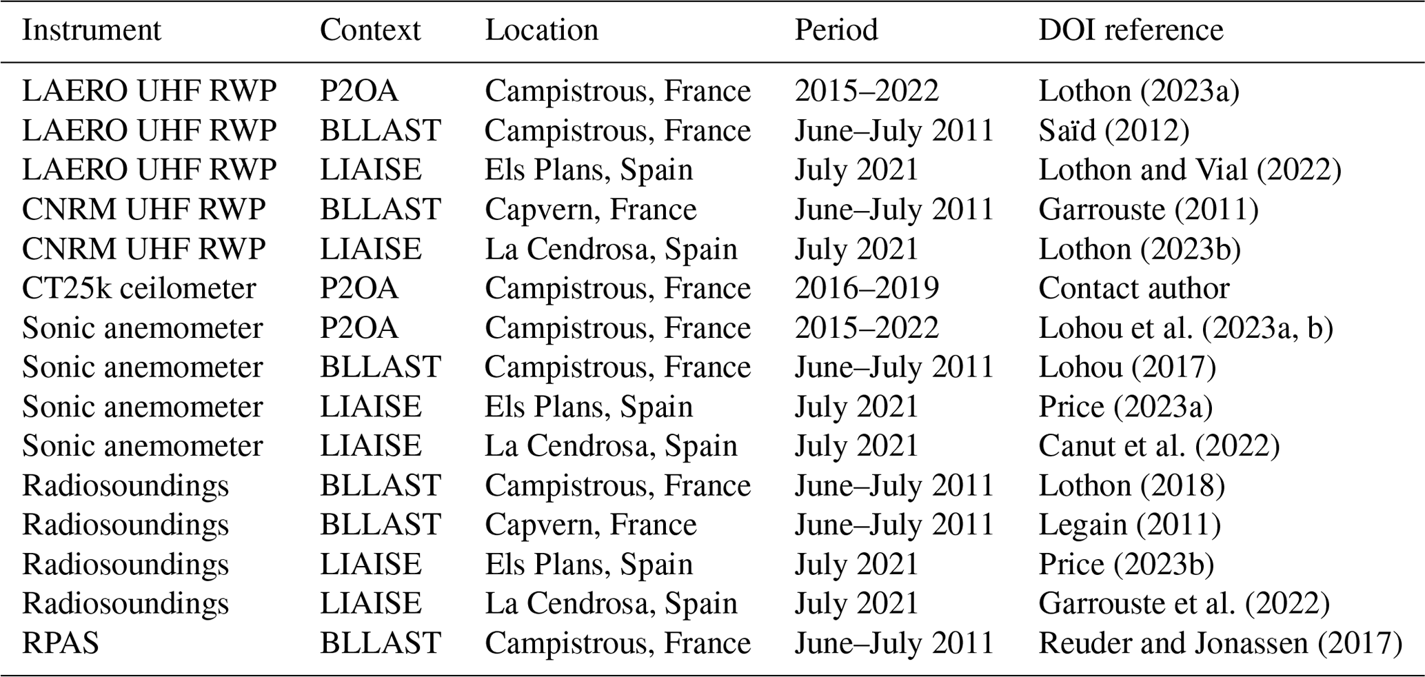
In conclusion, we also show that CALOTRITON is not specific to one UHF RWP and one observational site.
With this new algorithm, the main objective of obtaining reliable estimates of Zi with a UHF RWP for the analysis of long-term series is met here, except for CBL thinner than 225 m.
CALOTRITON uses two surface sensors in addition to the RWP: a humidity sensor at 2 m and a sonic anemometer for the evaluation of the sensible heat flux. We have seen that CALOTRITON can give satisfying results without the sensible heat flux input. The use of the humidity sensor allows for strong restriction of the attributions, especially in the presence of low stratus and fog. It thus remains useful and a low-cost and easy-to-use input. If this sensor is missing, CALOTRITON will likely attribute inaccurate Zi estimates on the top of the fog when it occurs. Using the sensible heat flux to restrict the estimations to days with significant fluxes (for example larger than 50 W m−2) can help to avoid the difficult CBL detection in winter (with very shallow or nonexistent CBL) or in certain strong foehn or heat wave cases (when the sensible heat fluxes may be low or even negative).
Relatively to the simpler, previously used algorithms for this profiler and to standard methods, CALOTRITON manages to deal with quite complex cases. Those “standard methods” are mainly based on catching the appropriate local maximum of with the help of temporal continuity. In CALOTRITON, the search for the first attribution of Zi at the first reliable UHF RWP gate is a significant progress consistent with the approach of Molod et al. (2015). Furthermore, taking into account both the higher reflectivity at inversions and the amount of turbulence within the CBL by use of the new key variable NPx allows for improvement in the attributions, in particular in the presence of clouds (the value of x being 3 or 4 seems the most appropriate). This was also found by Bianco and Wilczak (2002) with a different innovative fuzzy logic approach.
The criterion of temporal continuity, which appears as a real need, sometimes induces errors. Indeed, the associated jump threshold that is tolerated for CBL growth is somehow arbitrary and prevents the potential abrupt growth in certain conditions. Using to allow for a higher growth limit in those specific conditions helps to better manage complex cases. This is another improvement introduced by CALOTRITON. However, this one can also induce errors, in particular in the morning, by attributing Zi at the height of residual layers. Using an additional median filter on could allow us to limit these errors by better considering a certain temporal continuity of . The definition of could itself be improved. It is by itself an interesting useful variable.
The comparison of CALOTRITON Zi estimates with in situ thermodynamic profiles has shown that there is no automatic method based on in situ thermodynamic profiles which can deal with the complexity of the atmospheric structure and that the subjective method remains the best one. Such a subjective approach was actually also considered to be a reference in Bianco et al. (2008) but applied to the RWP variables.
CALOTRITON is definitely not a simple algorithm, but this actually reveals the need to adapt to the high complexity of the lower-atmosphere vertical structure. Bianco et al. (2008) proposed an improved algorithm relative to Bianco and Wilczak (2002) with more complexity added, which demonstrates this need for complexity and adjustments to optimize the understanding and detection of the appropriate interface. The flag system and various types of Zi estimates proposed in CALOTRITON allow us to express and document this vertical structure complexity while giving information on the quality and difficulty of the Zi estimations. In complex cases, characterizing the convective boundary layer by a single height may actually not be appropriate, in particular in the presence of TIBL, where it is difficult to determine (and even define) Zi even based on in situ thermodynamical data. It becomes very difficult to statistically qualify CALOTRITON attributions in such cases. Over the 8-year time series of the UHF RWP at P2OA, we find that 17 % of the days have more than 75 % of their Zi estimates with QF =1. This means that about 17 % of the days are quite close to textbook cases, with high confidence in CALOTRITON Zi estimates. In contrast, at Els Plans during the LIAISE campaign none of the days present QF =1 for more than 75 % of the time of day. That is why there is no simple textbook case in this area during the LIAISE summer campaign.
The use of the different Zi estimates by CALOTRITON is also of large interest for documenting the complex structure of the CBL, like the one found both in P2OA (at the foothills of the Pyrenees ridge) and at LIAISE (with the influence of the sea and the mountain at mesoscale). Moreover, it should only be used for statistical purposes with caution. One can, for example, estimate the occurrence of significant differences between and . At P2OA during the 8-year time series we find that only 3 % of the days show a significant difference between both estimates for more than 25 % of the time. This would mean that TIBLs are not very frequent at P2OA. In contrast, at Els Plan during LIAISE we find that 26 % of the days to be this way, which likely means that TIBLs occurred very frequently during the LIAISE campaign. One can also estimate the occurrence of differences between and ; at P2OA, over the 8-year time series, 72 % of the days show a significant difference between both variables for more than 25 % of each day. Those days can be related to the high occurrence of cloud layers above the CBL top, which generate inversions. At Els Plans during LIAISE this number reaches 92 %, which likely means that there are established upper inversions in the LIAISE area. Those preliminary statistics reveal the high complexity of the LIAISE study area and the potential of the CALOTRITON various estimates and flags. However, case-by-case studies and further analyses are needed to help us with qualifying this potential.
CALOTRITON code is available from the authors upon request.
Table 6 presents the list of available datasets, with DOIs and references. The CT25k ceilometer data are available from the authors upon request.
AP is the main author of the CALOTRITON algorithm, tackling conception, coding, tests, evaluation, and data analysis. He is also the main writer of the article. ML supervised the work and analysis and helped with the writing. She is the principal investigator of the Laboratoire d’Aérologie's ultra-high-frequency radar wind profiler (LAERO UHF RWP). JA and PYM are the coordinators of the funding contract and collaborated to do the work. BC is the author of the initial code for the UHF RWP data process and of the previous algorithm for Zi estimates. He helped with the algorithm conception. SD is responsible for the P2OA-CRA instrumentation and data. She and AV helped with the instrumentation maintenance, data process, and data availability. YB operated the LAERO UHF RWP at P2OA and during field experiments and helped with the operation of the CNRM UHF RWP during LIAISE. FL is the principal investigator of the 60 m tower and contributed to the writing. GC was the lead of the instrumental deployment during LIAISE and especially of the CNRM instruments installed at La Cendrosa. JB was responsible for the deployment of radiosoundings at Els Plans during LIAISE and contributed to the writing. JR was the PI of SUMO RPAS during BLLAST and contributed to the writing.
The contact author has declared that none of the authors has any competing interests.
Publisher’s note: Copernicus Publications remains neutral with regard to jurisdictional claims made in the text, published maps, institutional affiliations, or any other geographical representation in this paper. While Copernicus Publications makes every effort to include appropriate place names, the final responsibility lies with the authors.
P2OA-CRA observation data were collected at the Pyrenean Platform for Observation of the Atmosphere (P2OA; https://p2oa.aeris-data.fr/, last access: 22 March 2024). P2OA is a component of the ACTRIS-Fr research infrastructure and benefits from the AERIS data centre (https://www.aeris-data.fr/, last access: 22 March 2024) for hosting service data.
The BLLAST field experiment was hosted by the instrumented site of Centre de Recherches Atmosphériques, Campistrous, France (Observatoire Midi-Pyrénées, Laboratoire d’Aérologie). BLLAST data are managed by SEDOO from the Observatoire Midi-Pyrénées. For the data collected during the LIAISE campaign, we acknowledge the contribution of Gilles André, Géraldine Pagan, Vinciane Unger, Alain Dabas, Alexandre Paci, and the GMEI/LISA team of CNRM UMR. We also acknowledge the contribution of Jeremy Price and the entire Met Office team involved in LIAISE.
The contribution of Joachim Reuder to this study was partially supported by the LOWT project funded by the Research Council of Norway (RCN) under project number 325294.
This study has been supported by the French Alternative Energies and Atomic Energy Commission (CEA) and the Université of Toulouse III, Paul Sabatier, Toulouse.
P2OA facilities and staff are funded and supported by University Paul Sabatier Toulouse III, France, and CNRS (Centre National de la Recherche Scientifique).
The 60 m tower is partly supported by the POCTEFA/FLUXPYR European programme.
The BLLAST field experiment was made possible thanks to the contribution of several institutions and other supporters: INSU CNRS (Institut National des Sciences de l'Univers, Centre national de la Recherche Scientifique, the LEFE-IDAO programme), Météo-France, Observatoire Midi-Pyrénées (University of Toulouse), EUFAR (the EUropean Facility for Airborne Research), and COST (European Cooperation in Science and Technology) ES0802. The field experiment would not have occurred without the contribution of all participating European and American research groups, which have all contributed in a significant manner (see https://bllast.aeris-data.fr/bllast-supports/, last access: 22 March 2024). The French ANR (Agence Nationale de la Recherche) supported the BLLAST analysis during the 2013–2015 BLLAST-A project.
The French contribution to the LIAISE project was supported by ANR HILIAISE and Météo-France.
This paper was edited by Laura Bianco and reviewed by two anonymous referees.
Angevine, W. M.: Atmospheric boundary layer height measurements with wind profilers: Successes and cautions, International Geoscience and Remote Sensing Symposium (IGARSS), 1, 197–198, https://doi.org/10.1109/igarss.2000.860466, 2000. a, b
Angevine, W. M., White, A. B., and Avery, S. K.: Boundary-layer depth and entrainment zone characterization with a boundary-layer profiler, Bound.-Lay. Meteorol., 68, 375–385, https://doi.org/10.1007/BF00706797, 1994. a, b, c
Bianco, L. and Wilczak, J. M.: Convective boundary layer depth: Improved measurement by Doppler radar wind profiler using fuzzy logic methods, J. Atmos. Ocean. Technol., 19, 1745–1758, https://doi.org/10.1175/1520-0426(2002)019<1745:CBLDIM>2.0.CO;2, 2002. a, b, c, d, e
Bianco, L., Wilczak, J. M., and White, A. B.: Convective boundary layer depth estimation from wind profilers: Statistical comparison between an automated algorithm and expert estimations, J. Atmos. Ocean. Technol., 25, 1397–1413, https://doi.org/10.1175/2008JTECHA981.1, 2008. a, b, c, d
Blay-Carreras, E., Pino, D., Vilà-Guerau de Arellano, J., van de Boer, A., De Coster, O., Darbieu, C., Hartogensis, O., Lohou, F., Lothon, M., and Pietersen, H.: Role of the residual layer and large-scale subsidence on the development and evolution of the convective boundary layer, Atmos. Chem. Phys., 14, 4515–4530, https://doi.org/10.5194/acp-14-4515-2014, 2014. a
Boone, A., Bellvert, J., Best, M., Brooke, J., Canut-Rocafort, G., Cuxart, J., Hartogensis, O., Le Moigne, P., Miró, J. R., Polcher, J., Price, J., Quintana Seguí, P., and Wooster, M.: Updates on the international Land Surface Interactions with the Atmosphere over the Iberian Semi-Arid Environment (LIAISE) Field Campaign, Gewex News, 31, 17–21, 2021. a, b, c
Caicedo, V., Rappenglück, B., Lefer, B., Morris, G., Toledo, D., and Delgado, R.: Comparison of aerosol lidar retrieval methods for boundary layer height detection using ceilometer aerosol backscatter data, Atmos. Meas. Tech., 10, 1609–1622, https://doi.org/10.5194/amt-10-1609-2017, 2017. a
Canut, G., Garrouste, O., and Etienne, J.-C.: LIAISE LA-CENDROSA CNRM MTO-1MIN L2, AERIS [data set], https://doi.org/10.25326/33, 2022. a
Cohn, S. A. and Angevine, W. M.: Boundary Layer Height and Entrainment Zone Thickness Measured by Lidars and Wind-Profiling Radars, J. Appl. Meteorol., 39, 1233–1247, https://doi.org/10.1175/1520-0450(2000)039<1233:BLHAEZ>2.0.CO;2, 2000. a
Collaud Coen, M., Praz, C., Haefele, A., Ruffieux, D., Kaufmann, P., and Calpini, B.: Determination and climatology of the planetary boundary layer height above the Swiss plateau by in situ and remote sensing measurements as well as by the COSMO-2 model, Atmos. Chem. Phys., 14, 13205–13221, https://doi.org/10.5194/acp-14-13205-2014, 2014. a, b, c
Compton, J. C., Delgado, R., Berkoff, T. A., and Hoff, R. M.: Determination of planetary boundary layer height on short spatial and temporal scales: A demonstration of the covariance wavelet transform in ground-based wind profiler and lidar measurements, J. Atmos. Ocean. Technol., 30, 1566–1575, https://doi.org/10.1175/JTECH-D-12-00116.1, 2013. a
Couvreux, F., Bazile, E., Canut, G., Seity, Y., Lothon, M., Lohou, F., Guichard, F., and Nilsson, E.: Boundary-layer turbulent processes and mesoscale variability represented by numerical weather prediction models during the BLLAST campaign, Atmos. Chem. Phys., 16, 8983–9002, https://doi.org/10.5194/acp-16-8983-2016, 2016. a, b, c
Davis, K. J., Gamage, N., Hagelberg, C., Kiemle, C., Lenschow, D., and Sullivan, P.: An objective method for deriving atmospheric structure from airborne lidar observations, J. Atmos. Ocean. Technol., 17, 1455–1468, https://doi.org/10.1175/1520-0426(2000)017<1455:AOMFDA>2.0.CO;2, 2000. a
Deardorff, J. W.: Theoretical expression for the countergradient vertical heat flux, J. Geophys. Res., 77, 5900–5904, https://doi.org/10.1029/jc077i030p05900, 1972. a
Doviak, R. and Zrnic, D.: Doppler Radar and Weather Observations, Elsevier, ISBN 9780122214226, https://doi.org/10.1016/C2009-0-22358-0, 1993. a
Duncan Jr., J. B., Bianco, L., Adler, B., Bell, T., Djalalova, I. V., Riihimaki, L., Sedlar, J., Smith, E. N., Turner, D. D., Wagner, T. J., and Wilczak, J. M.: Evaluating convective planetary boundary layer height estimations resolved by both active and passive remote sensing instruments during the CHEESEHEAD19 field campaign, Atmos. Meas. Tech., 15, 2479–2502, https://doi.org/10.5194/amt-15-2479-2022, 2022. a
Durand, P., Druilhet, A., and Briere, S.: A Sea-Land Transition Observed during the COAST Experiment, J. Atmos. Sci., 46, 96–116, https://doi.org/10.1175/1520-0469(1989)046<0096:ASLTOD>2.0.CO;2, 1989. a
Frehlich, R., Meillier, Y., Jensen, M. L., Balsley, B., and Sharman, R.: Measurements of Boundary Layer Profiles in an Urban Environment, J. Appl. Meteorol. Climatol., 45, 821–837, https://doi.org/10.1175/JAM2368.1, 2006. a, b
Garrouste, O.: UHF CNRM Site 2, AERIS [data set], https://doi.org/10.6096/bllast.uhf.site2, 2011. a
Garrouste, O., Canut, G., and Roy, A.: LIAISE LA-CENDROSA CNRM RS L2, AERIS [data set], https://doi.org/10.25326/322, 2022. a
Grimsdell, A. W. and Angevine, W. M.: Convective boundary layer height measurement with wind profilers and comparison to cloud base, J. Atmos. Ocean. Technol., 15, 1331–1338, https://doi.org/10.1175/1520-0426(1998)015<1331:CBLHMW>2.0.CO;2. , 1998. a
Grimsdell, A. W. and Angevine, W. M.: Observations of the Afternoon Transition of the Convective Boundary Layer, J. Appl. Meteorol., 41, 3–11, https://doi.org/10.1175/1520-0450(2002)041<0003:OOTATO>2.0.CO;2, 2002. a, b
Haeffelin, M., Angelini, F., Morille, Y., Martucci, G., Frey, S., Gobbi, G. P., Lolli, S., O'Dowd, C. D., Sauvage, L., Xueref-Rémy, I., Wastine, B., and Feist, D. G.: Evaluation of Mixing-Height Retrievals from Automatic Profiling Lidars and Ceilometers in View of Future Integrated Networks in Europe, Bound.-Lay. Meteorol., 143, 49–75, https://doi.org/10.1007/s10546-011-9643-z, 2012. a
Hanna, S. R.: The thickness of the planetary boundary layer, Atmos. Environ., 3, 519–536, https://doi.org/10.1016/0004-6981(69)90042-0, 1969. a
Hennemuth, B. and Lammert, A.: Determination of the atmospheric boundary layer height from radiosonde and lidar backscatter, Bound.-Lay. Meteorol., 120, 181–200, https://doi.org/10.1007/s10546-005-9035-3, 2006. a, b, c
Heo, B. H., Jacoby-Koaly, S., Kim, K. E., Campistron, B., Benech, B., and Jung, E. S.: Use of the Doppler spectral width to improve the estimation of the convective boundary layer height from UHF wind profiler observations, J. Atmos. Ocean. Technol., 20, 408–424, https://doi.org/10.1175/1520-0426(2003)020<0408:UOTDSW>2.0.CO;2, 2003. a, b, c, d
Holzworth, G. C.: Estimates of mean maximum mixing depths in the contiguous united states, Mon. Weather Rev., 92, 235–242, https://doi.org/10.1175/1520-0493(1964)092<0235:EOMMMD>2.3.CO;2, 1964. a
Jacoby-Koaly, S.: Application d'un radar profileur de vent UHF à l'étude de la couche limite atmosphérique, Ph.D. thesis, thèse de doctorat dirigée par Campistron, Bernard Physique de l'atmosphère Toulouse 3 2000, http://www.theses.fr/2000TOU30144 (last access: 22 March 2024), 2000. a, b
Jacoby-Koaly, S., Campistron, B., Bernard, S., Bénech, B., Ardhuin-Girard, F., Dessens, J., Dupont, E., and Carissimo, B.: Turbulent Dissipation Rate In The Boundary Layer Via UHF Wind Profiler Doppler Spectral Width Measurements, Bound.-Lay. Meteorol., 103, 361–389, https://doi.org/10.1023/A:1014985111855, 2002. a, b, c, d, e
Jiménez, M. A., Grau, A., Martínez-Villagrasa, D., and Cuxart, J.: Characterization of the marine-air intrusion Marinada in the eastern Ebro sub-basin, Int. J. Climatol., 43, 7682–7699. https://doi.org/10.1002/joc.8287, 2023. a, b
Kossmann, M., Gtlin, R. V., Corsmeier, U., Vogel, B., Fiedler, F., Binder, H.-J., Kalthoff, N., and Beyrich, F.: Aspects of the convective boundary layer structure over complex terrain, Atmos. Environ., 32, 1323–1348, https://doi.org/10.1016/S1352-2310(97)00271-9, 1998. a
Kotthaus, S., Bravo-Aranda, J. A., Collaud Coen, M., Guerrero-Rascado, J. L., Costa, M. J., Cimini, D., O'Connor, E. J., Hervo, M., Alados-Arboledas, L., Jiménez-Portaz, M., Mona, L., Ruffieux, D., Illingworth, A., and Haeffelin, M.: Atmospheric boundary layer height from ground-based remote sensing: a review of capabilities and limitations, Atmos. Meas. Tech., 16, 433–479, https://doi.org/10.5194/amt-16-433-2023, 2023. a, b
Legain, D.: Frequent radiosoundings Site 2, AERIS [data set], https://doi.org/10.6096/bllast.frequentsoundingssite2, 2011. a
Legain, D., Bousquet, O., Douffet, T., Tzanos, D., Moulin, E., Barrie, J., and Renard, J.-B.: High-frequency boundary layer profiling with reusable radiosondes, Atmos. Meas. Tech., 6, 2195–2205, https://doi.org/10.5194/amt-6-2195-2013, 2013. a
Liu, Z., Barlow, J. F., Chan, P.-W., Fung, J., Li, Y., Ren, C., Mak, H., and Ng, E.: A Review of Progress and Applications of Pulsed Doppler Wind LiDARs, Remote Sens., 11, 2522, https://doi.org/10.3390/rs11212522, 2019. a
Lohou, F.: Meteorological parameters and flux, AERIS [data set], https://doi.org/10.6096/bllast.60mtower.meteo, 2017. a
Lohou, F., Derrien, S., Vial, A., Philibert, A., Gabella, O., Said, F., Pique, E., and Meyerfeld, Y.: P2OA-CRA station – Turbulence measurements – L2A, ERIS, https://doi.org/10.25326/550, 2023a. a
Lohou, F., Derrien, S., Vial, A., Philibert, A., Gabella, O., Said, F., Pique, E., and Meyerfeld, Y.: 60 m Tower – P2OA-CRA station – Meteorological variables – L2A, AERIS [data set], https://doi.org/10.25326/551, 2023b. a
Lothon, M.: MODEM Radiosoundings Site 1, AERIS [data set], https://doi.org/10.6096/bllast.modem, 2018. a
Lothon, M.: UHF-RADAR – P2OA-CRA station – Level 2A wind profiles – Monthly files, AERIS [data set], https://doi.org/10.25326/563, 2023a. a
Lothon, M.: LIAISE LA-CENDROSA CNRM UHFWindProfiler-LowMode L2, AERIS [data set], https://doi.org/10.25326/471, 2023b. a
Lothon, M. and Vial, A.: LIAISE ELS-PLANS LAERO UHFWindProfiler-LowMode L2, AERIS [data set], https://doi.org/10.25326/363, 2022. a
Lothon, M., Lenschow, D. H., and Mayor, S. D.: Coherence and scale of vertical velocity in the convective boundary layer from a Doppler lidar, Bound.-Lay. Meteorol., 121, 521–536, https://doi.org/10.1007/s10546-006-9077-1, 2006. a
Lothon, M., Lohou, F., Pino, D., Couvreux, F., Pardyjak, E. R., Reuder, J., Vilà-Guerau de Arellano, J., Durand, P., Hartogensis, O., Legain, D., Augustin, P., Gioli, B., Lenschow, D. H., Faloona, I., Yagüe, C., Alexander, D. C., Angevine, W. M., Bargain, E., Barrié, J., Bazile, E., Bezombes, Y., Blay-Carreras, E., van de Boer, A., Boichard, J. L., Bourdon, A., Butet, A., Campistron, B., de Coster, O., Cuxart, J., Dabas, A., Darbieu, C., Deboudt, K., Delbarre, H., Derrien, S., Flament, P., Fourmentin, M., Garai, A., Gibert, F., Graf, A., Groebner, J., Guichard, F., Jiménez, M. A., Jonassen, M., van den Kroonenberg, A., Magliulo, V., Martin, S., Martinez, D., Mastrorillo, L., Moene, A. F., Molinos, F., Moulin, E., Pietersen, H. P., Piguet, B., Pique, E., Román-Cascón, C., Rufin-Soler, C., Saïd, F., Sastre-Marugán, M., Seity, Y., Steeneveld, G. J., Toscano, P., Traullé, O., Tzanos, D., Wacker, S., Wildmann, N., and Zaldei, A.: The BLLAST field experiment: Boundary-Layer Late Afternoon and Sunset Turbulence, Atmos. Chem. Phys., 14, 10931–10960, https://doi.org/10.5194/acp-14-10931-2014, 2014. a, b, c, d
Lothon, M., Gheusi, F., Lohou, F., Pont, V., Derrien, S., Bezombes, Y., Leclerc, E., Vial, A., Athier, G., Jambert, C., Gardrat, E., Andriatiana, A., Meyerfeld, Y., Campistron, B., Saïd, F., Philibert, A., Stark, F., Estrampes, J.-B., Pique, E., Guesdon, F., Bret, G., Lacassagne, F., Guesdon, L., Gueffier, J., Jeroen, S., and Zaïda, G. K.: The long-term dataset of the Pyrenean Platform for Observation of the Atmosphere, Earth Syst. Sci. Data Discuss., submitted, 2024. a, b
Min, J.-S., Park, M.-S., Chae, J.-H., and Kang, M.: Integrated System for Atmospheric Boundary Layer Height Estimation (ISABLE) using a ceilometer and microwave radiometer, Atmos. Meas. Tech., 13, 6965–6987, https://doi.org/10.5194/amt-13-6965-2020, 2020. a
Molod, A., Salmun, H., and Dempsey, M.: Estimating planetary boundary layer heights from NOAA Profiler Network wind profiler data, J. Atmos. Ocean. Technol., 32, 1545–1561, https://doi.org/10.1175/JTECH-D-14-00155.1, 2015. a, b, c, d
Nilsson, E., Lohou, F., Lothon, M., Pardyjak, E., Mahrt, L., and Darbieu, C.: Turbulence kinetic energy budget during the afternoon transition – Part 1: Observed surface TKE budget and boundary layer description for 10 intensive observation period days, Atmos. Chem. Phys., 16, 8849–8872, https://doi.org/10.5194/acp-16-8849-2016, 2016a. a
Nilsson, E., Lothon, M., Lohou, F., Pardyjak, E., Hartogensis, O., and Darbieu, C.: Turbulence kinetic energy budget during the afternoon transition – Part 2: A simple TKE model, Atmos. Chem. Phys., 16, 8873–8898, https://doi.org/10.5194/acp-16-8873-2016, 2016b. a, b
Pino, D., Jonker, H. J. J., Arellano, J. V.-G. D., and Dosio, A.: Role of Shear and the Inversion Strength During Sunset Turbulence Over Land: Characteristic Length Scales, Bound.-Lay. Meteorol., 121, 537–556, https://doi.org/10.1007/s10546-006-9080-6, 2006. a
Price, J.: LIAISE ELS-PLANS UKMO MTO-30MIN L2, AERIS [data set], https://doi.org/10.25326/430, 2023a. a
Price, J.: LIAISE ELS-PLANS UKMO radiosondes L1, AERIS [data set], https://doi.org/10.25326/429, 2023b. a
Reuder, J. and Jonassen, M.: SUMO, AERIS [data set], https://doi.org/10.25326/469, 2017. a
Reuder, J., Båserud, L., Jonassen, M. O., Kral, S. T., and Müller, M.: Exploring the potential of the RPA system SUMO for multipurpose boundary-layer missions during the BLLAST campaign, Atmos. Meas. Tech., 9, 2675–2688, https://doi.org/10.5194/amt-9-2675-2016, 2016. a
Saïd, F.: LA Site 1, AERIS [data set], https://doi.org/10.6096/bllast.uhf.site1, 2012. a
Seibert, P., Beyrich, F., Gryning, S.-E., Joffre, S., Rasmussen, A., and Tercier, P.: Review and intercomparison of operational methods for the determination of the mixing height, Atmos. Environ., 34, 1001–1027, https://doi.org/10.1016/S1352-2310(99)00349-0, 2000. a, b
Stull, R. B.: An Introduction to Boundary Layer Meteorology, Springer Netherlands, ISBN 978-90-277-2769-5, https://doi.org/10.1007/978-94-009-3027-8, 1988. a, b, c
Turner, D. D. and Löhnert, U.: Ground-based temperature and humidity profiling: combining active and passive remote sensors, Atmos. Meas. Tech., 14, 3033–3048, https://doi.org/10.5194/amt-14-3033-2021, 2021. a
Wadteufel, P. and Corbin, H.: On the analysis of single-Doppler data, J. App. Meteor., 18, 523–542, https://doi.org/10.1175/1520-0450(1979)018<0532:OTAOSD>2.0.CO;2, 1979. a
White, A. B.: Mixing Depth Detection Using 915-MHz Radar Reflectivity Data, Proceedings of the 8th Symposium on Meteorological Observations and Instrumentation, Anaheim, CA, American Meteorological Society, 45 Beacon St., Boston, MA, 248–250, Anaheim, CA, USA, 1993., 1993. a
ACTRIS-Fr is the French component of the European Aerosol, Cloud and Trace Gases Research Infrastructure (ACTRIS), https://www.actris.fr/ (last access: 22 March 2024).
https://p2oa.aeris-data.fr/ (last access: 22 March 2024).
Laboratoire d'Aérologie, Université de Toulouse, CNRS, UPS, France.
- Abstract
- Introduction
- Instrumentation and data
- The CALOTRITON algorithm
- Illustrative case studies
- Validation of CALOTRITON with in situ measurements
- Summary and discussion
- Code availability
- Data availability
- Author contributions
- Competing interests
- Disclaimer
- Acknowledgements
- Financial support
- Review statement
- References