An improved OMI ozone profile research product version 2.0 with collection 4 L1b data and algorithm updates

We describe the new and improved version 2 of the ozone profile research product from the Ozone Monitoring Instrument (OMI) on the Aura satellite. One of the major changes is to switch the OMI L1b data from collection 3 to the recent collection 4 as well as the accompanying auxiliary datasets. The algorithm details are updated on radiative transfer model calculation and measurement calibrations, along with the input changes in meteorological data, and with the use of a tropopause-based ozone profile climatology, an improved high-resolution solar reference spectrum, and a recent ozone absorption cross-section dataset. A super Gaussian is applied to better represent OMI slit functions instead of a normal Gaussian. The effect of slit function errors on the spectral residuals is further accounted for as pseudo-absorbers in the iterative fit process. The OMI irradiances are averaged into monthly composites to reduce noise uncertainties in OMI daily measurements and to cancel out the temporal variations of instrument characteristics that are common in both radiance and irradiance measurements, which was previously neglected due to use of climatological composites. The empirical soft calibration spectra are re-derived to be consistent with the updated implementations and derived annually to remove the time-varying systematic biases between measured and simulated radiances. The “common mode” correction spectra are derived from remaining residual spectra after soft calibration as a function of solar zenith angle. The common mode is included as a pseudo-absorber in the iterative fit process, which helps to reduce the discrepancies of ozone retrieval accuracy between lower and higher solar zenith angles and between nadir and off-nadir pixels. Validation with ozonesonde measurements demonstrates the improvements of ozone profile retrievals in the troposphere, especially around the tropopause. The retrieval quality of tropospheric column ozone is improved with respect to the seasonal consistency between winter and summer as well as the long-term consistency before and after the row-anomaly occurrence.

1 Introduction

The Smithsonian Astrophysical Observatory (SAO) ozone profile algorithm was originally developed to retrieve ozone profiles with sensitivity down to the lower troposphere from Global Ozone Monitoring Experiment (GOME) measurements (Liu et al., 2005) and has been continuously adapted to the Ozone Monitoring Instrument (OMI) (Liu et al., 2010), GOME/2A (Cai et al., 2012), the Ozone Mapping and Profiler Suite (OMPS) (Bak et al., 2017), the TROPOspheric Monitoring Instrument (TROPOMI) (Zhao et al., 2021), the Geostationary Environment Monitoring Spectrometer (GEMS) (Bak et al., 2019a), and Tropospheric Emissions: Monitoring of Pollution (TEMPO) (Zoogman et al., 2017). The SAO algorithm has been put into production in NASA's OMI Science Investigator-led Processing System (SIPS) to create the OMI ozone profile research product titled OMPROFOZ v0.93 (referred to as version 1 hereafter) that is publicly distributed via the Aura Validation Data Center (AVDC) (https://avdc.gsfc.nasa.gov/pub/data/satellite/Aura/OMI/V03/L2/OMPROFOZ/, last access: 12 March 2024). The OMPROFOZ product has contributed to a better understanding of chemical and dynamical ozone variability associated with anthropogenic pollution over central and eastern China (Hayashida et al., 2015; Wei et al., 2022), transport of anthropogenic pollution in free troposphere (Walker et al., 2010), and stratospheric ozone intrusion (Kuang et al., 2017), as well as ozone concentration changes in the Asian summer monsoon (Lu et al., 2018; Luo et al., 2018). Moreover, this product has been used to quantify the global tropospheric budget of ozone and to evaluate how well current chemistry–climate models reproduce the observations (Hu et al., 2017; Zhang et al., 2010). OMI shows progressively low optical degradation over the mission, with a change of ∼ 3 % in the radiance over roughly 1.5 decades (Kleipool et al., 2022). However, the long-term reliability of the OMPROFOZ product, particularly concerning tropospheric ozone measurements, remains susceptible to optical instrument degradation (Gaudel et al., 2018; Huang et al., 2018, 2017). Huang et al. (2018, 2017) conducted an in-depth assessment of 10 years of the OMPROFOZ product through spatiotemporal validation using a global reference dataset collected from balloon-borne ozonesondes and the spaceborne Microwave Limb Sounder (MLS), which is one of the payloads on board the Aura satellite, along with OMI. They concluded that there are noticeable discrepancies in time series of data quality and suggested the need to address the spatiotemporal variations of the retrieval performance and the related cross-track dependency. Since the first release of OMPROFOZ data, implementation details have been externally refined to improve the retrieval quality. Bak et al. (2013) demonstrated improvements of ozone profile retrievals around the extratropical tropopause region by better constraining climatological a priori information. To better represent an instrument spectral response function (ISRF), Sun et al. (2017) employed a super Gaussian function which can represent more complex shapes compared to a classical Gaussian function. The slit function linearization was experimented with in Bak et al. (2019b) to account for the effects of errors in slit function parameters on the spectral fit residuals. Moreover, the best spectroscopic inputs were investigated with respect to the ozone cross-section (Bak et al., 2020; Liu et al., 2013) and the high-resolution solar reference spectrum (Bak et al., 2022). To accelerate the time-consuming radiative transfer (RT) calculation, an RT model based on principal component analysis (PCA) was employed as a forward model with the correction scheme of RT approximation errors using lookup tables (LUTs) (Bak et al., 2021). The updates to radiometric corrections were made with the time-dependent soft calibration and solar-zenith-angle-dependent common mode correction, improving the spatiotemporal consistency of retrieval quality, which are detailed in this paper. Individual refinements mentioned above are incorporated in the OMPROFOZ version 2 (v2) algorithm, along with the switch of OMI L1b data product from collection 3 to collection 4. Note that OMI measurements have been reprocessed to deliver the recent collection 4 dataset, which supersedes and improves the collection 3 with respect to the ongoing instrument effects and optical degradations, drifts in electronic gain, and pixel quality flagging (Kleipool et al., 2022).

In this paper we describe updates made in the OMI ozone profile algorithm, discuss their impact on spectral fit and ozone profile retrievals, and provide an initial quantitative assessment of tropospheric ozone columns with respect to their long-term consistency. Section 2 describes OMI L1b and auxiliary products used in retrieving ozone profiles, along with the retrieval methodology and OMPROFOZ v2 product. In Sect. 3 the updates of implementation details are specified and verified. Section 4 presents the validation results using ozonesonde measurements. This paper is summarized and concluded in Sect. 5.

2 Description of the SAO OMI ozone profile algorithm and OMPROFOZ product

2.1 OMI products

Table 1 lists the OMI standard or auxiliary products used in reprocessing OMI ozone profiles, which are publicly available through NASA's Goddard Earth Sciences Data and Information Services Center (GES DISC). OMI is a nadir-viewing UV and visible spectrometer in which two-dimensional (spectral × spatial) charged-coupled device (CCD) detectors are employed. The collection 4 L0-1b processor was newly built based on the TROPOMI L0-1b processor at the OMI SIPS, which produces radiometrically calibrated and geolocated solar irradiances and earthshine radiances from the raw sensor measurements. Insights learned from the usage of OMI collection 3 data over the past 17 years are leveraged to correct optical and electronic aging and improve pixel quality flagging. The details of switching from collection 3 to collection 4 can be found in Kleipool et al. (2022). The OML1BIRR provides the daily averaged irradiance measurements. The OML1BRUG contains Earth view spectral radiances taken in the global mode from the UV detector. To increase a signal-to-noise ratio (SNR) at shorter UV wavelengths, a measured spectrum is divided into two sub-channels at ∼ 310 nm and then the spatial resolution of the shorter wavelength is degraded by a factor of 2 in cross-track pixels, resulting in 48 and 24 km at nadir in band 1 (UV-1, 159 channels in 264–311 nm) and in band 2 (UV-2, 557 channels in 307–383 nm), respectively. The spatial resolution is 13 km in the flight direction. Cloud information is taken from OMCLDO2 based on the spectral fitting of the O₂–O₂ absorption band at 477 nm, while a climatological surface albedo is taken from OMLER. The OMUANC is a new ancillary product, geo-collocated to UV2 spatial pixels, developed to support the production of OMI L2 products in the framework of collection 4. This product contains flags to identify snow–ice pixels based on the Near real-time Ice and Snow Extent (NISE) data and to screen out anomaly rows based on the NASA flagging scheme. The row anomaly (RA) is an anomaly which affects OMI measurements at all wavelengths for some particular rows of the CCD detector. Only two of OMI's 60 rows in the UV2 image were initially affected in 2007, but the anomalies have become more serious since January 2009 (∼ 30%), spreading to ∼ 50 % (rows 25–55) during the period of 2010–2012. There is no reliable correction scheme for RA-affected measurements, and therefore flagging the row anomalies as bad data is crucial to ensure the L2 product quality. An RA flag is available from both OML1BRUG and OMUANC. The former relies on the analysis of features observed in radiance measurements to identify the row-anomaly-contaminated pixels, referred as to the KNMI flagging method, which remains unchanged from collection 3 to 4 (Ludewig et al., 2021). The latter is based on a statistical analysis of errors detected in the OMI TOMS-like total column ozone data, referred as to the NASA flagging method. According to Schenkeveld et al. (2017), who compared the KNMI and NASA flagging results in the UV2 channel, the two methods produce consistent flagging results over the full course of the OMI mission, but the NASA method is likely to be stricter and more reliable. In this paper, row anomalies are filtered out when either OML1BRUG (UV2 only) or OMUANC flags are raised. The OMUFPMET and OMUFPSLV supply meteorological fields at OMI overpass positions, which is further detailed in Sect. 3.2 where the updates to meteorological inputs in OMPROFOZ are verified. We applied the OMI total column ozone product (OMTO3d) to adjust the ozone profile shape used as an input for deriving empirical correction spectra (Sect. 3.8).

Table 1 Input list of OMI data.

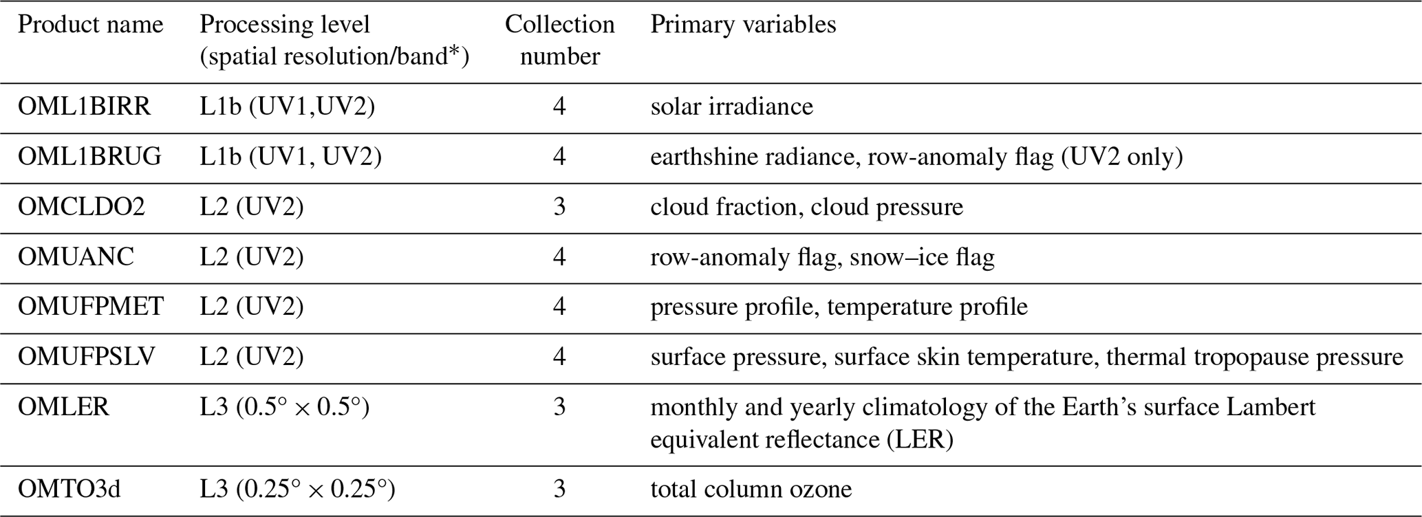
^* UV1, UV2, and VIS represent bands and their corresponding spatial resolutions (except for OML1BIRR) of 13 × 48, 13 × 24, and 13 × 24 km² at nadir, respectively.

2.2 OMPROFOZ algorithm

As depicted in Fig. 1, our algorithm is composed of an inversion based on optimal estimation (OE) (Rodgers, 2000), radiative transfer (forward) model simulations, and state-of-the-art calibrations. We have two spectral windows: one spanning 270–309 nm in the UV-1 band and another spanning 312–330 nm in the UV-2 band. Two UV-2 spatial pixels are co-added to match UV-1 spatial resolution in the cross-track direction. To meet the computational budget, OMI measurements were spatially co-added in the flight direction, reducing the spatial resolution to 48 × 52 km² in the earlier data processing. In the new data processing, OMPROFOZ will be released at 48 × 26 km², owing to the speed-up of radiative transfer calculations described in Sect. 3.7. In the calibration process, a cross-correlation technique is implemented to characterize in-orbit slit functions and wavelength shift errors (Δλ) using a well-calibrated, high-resolution solar reference spectrum. The empirical correction or so-called soft calibration is applied to eliminate the systematic measurement biases in the wavelength range of 270–330 nm for ozone fitting and around 347 nm for the initial surface albedo and cloud fitting. This correction was previously applied dependent on wavelength and cross-track position but currently updated to enable a correction for time-dependent degradation (Sect. 3.8).

Figure 1 Flowchart for retrieving ozone profiles with optimal-estimation-based inversion.

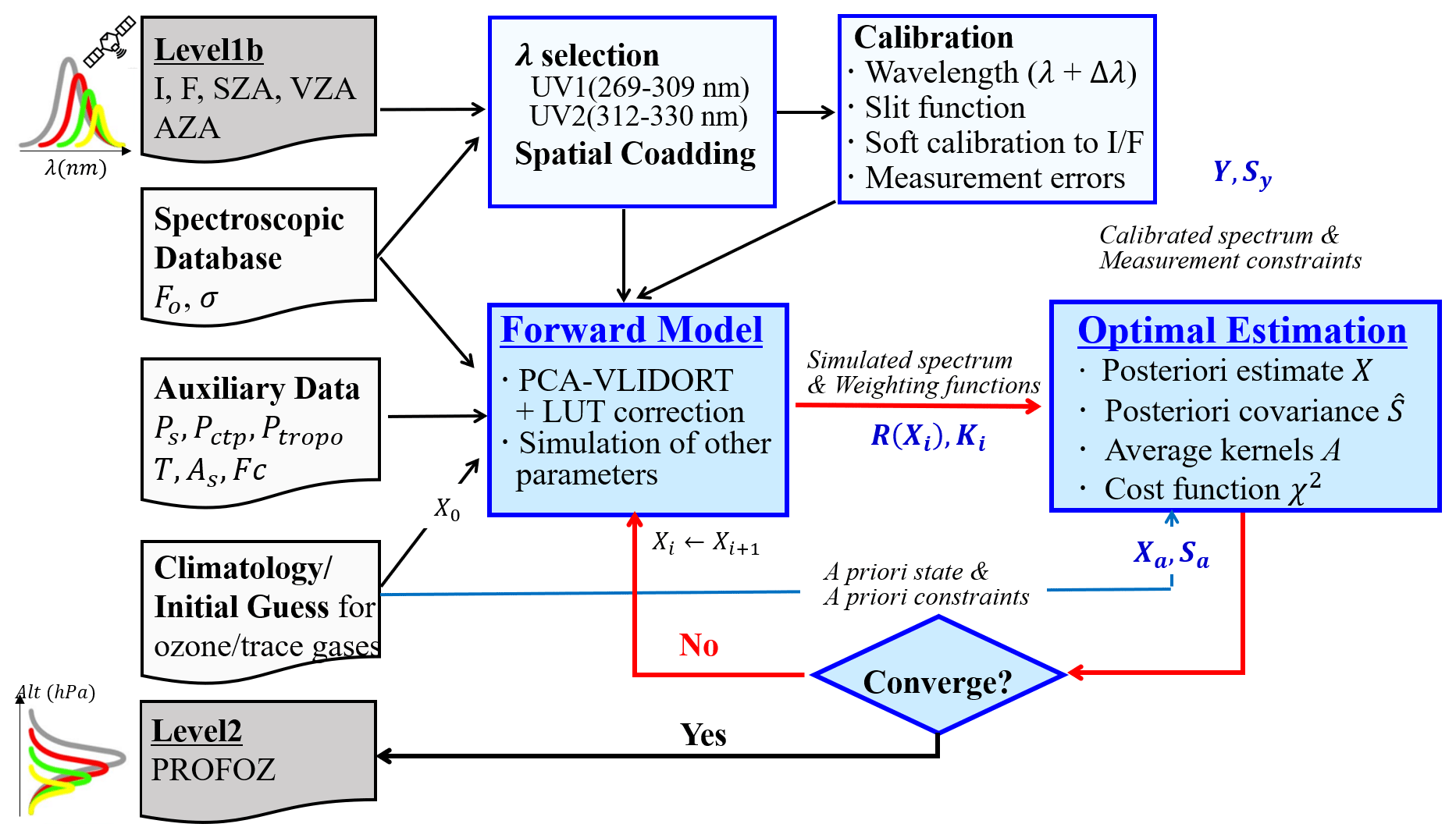
This OE-based inversion is physically regularized toward minimizing the difference between a measured spectrum Y and a spectrum that is simulated by the forward model R(X), constrained by measurement error covariance matrix S_y and statistically regularized by an a priori state vector X_a and error covariance matrix S_a. The solution at iteration step i+1 is written as

$$\begin{array}{}\text{(1)}& \begin{array}{rl}{\mathit{X}}_{i+\mathrm{1}}& ={\mathit{X}}_i+{\left({\mathbf{K}}_i^T{\mathbf{S}}_y^{-\mathrm{1}}{\mathbf{K}}_i+{\mathbf{S}}_{\mathrm{a}}^{-\mathrm{1}}\right)}^{-\mathrm{1}}\\ & \left[{\mathbf{K}}_i^T{\mathbf{S}}_y^{-\mathrm{1}}\left(\mathit{Y}-\mathbf{R}\left({\mathit{X}}_i\right)\right)-{\mathbf{S}}_{\mathrm{a}}^{-\mathrm{1}}\left({\mathit{X}}_i-{\mathit{X}}_{\mathrm{a}}\right)\right],\end{array}\end{array}$$

where each component of K is the derivative of the forward model, called the Jacobians or weighting function matrix. Y is composed of the logarithm of the sun-normalized radiance. To construct S_y, the normalized random noise errors of radiance and irradiance taken from OMI L1b products are summed up as total measurement errors. The measurement errors are typically underestimated and then noise floors (0.4 % below 310 nm, 0.15 %–0.2 % above) are imposed on as a minimum value. S_y is a diagonal matrix, assuming that measurement errors are uncorrelated among wavelengths.

The optimal estimate is iteratively updated until convergence when the relative change in the cost function between previous and current iterations is less than 1.0 %. The cost function χ² is given by

$$\begin{array}{}\text{(2)}& \begin{array}{rl}{\mathit{\chi }}^{\mathrm{2}}& ={∥{\mathbf{S}}_y^{-\frac{\mathrm{1}}{\mathrm{2}}}\left\{{\mathbf{K}}_i\left({\mathit{X}}_{i+\mathrm{1}}-{\mathit{X}}_i\right)-\left[\mathit{Y}-\mathbf{R}\left({\mathit{X}}_i\right)\right]\right\}∥}_{\mathrm{2}}^{\mathrm{2}}\\ & +{∥{\mathbf{S}}_{\mathrm{a}}^{-\frac{\mathrm{1}}{\mathrm{2}}}\left({\mathit{X}}_{i+\mathrm{1}}-{\mathit{X}}_{\mathrm{a}}\right)∥}_{\mathrm{2}}^{\mathrm{2}},\end{array}\end{array}$$

where $\Vert {\Vert }_{\mathrm{2}}^{\mathrm{2}}$ denotes the sum of each element squared. The maximum number of iterations is set to be 10 against the divergence. Typically, it takes two to three iterations to converge, but increasing to six to seven for thick clouds. Table 2 provides fitting variables for OMPROFOZ v2, along with their a priori values and a priori errors. In comparison to the previous version, three kinds of parameters are newly added to implement the slit function linearization (slit width coefficient, shape factor coefficient) and common mode correction as a pseudo-absorber. The a priori value and error are set empirically for spectroscopic parameters and are taken from climatological datasets for geophysical parameters such as atmospheric ozone and surface albedo. They are assumed to be uncorrelated between fitting parameters, except for atmospheric profiles with a correlation length of 6 km, which gives

$${\mathbf{S}}_{\mathrm{a}}(i,j)={\mathit{\sigma }}_i^{\mathrm{a}}{\mathit{\sigma }}_j^{\mathrm{a}}\exp \left(-\mathrm{|}i-j\mathrm{|}/\mathrm{6}\right),$$

where σ^a is a priori error, with i and j being layer numbers. The cloud fraction is initially taken from OMCLDO2 and fitted at 347 nm together with initial surface albedo taken from OMLER.

Table 2 List of fitting variables, a priori values, and a priori errors. A correlation length of 6 km is used to construct the a priori covariance matrix for ozone variables. All the other variables are assumed to be uncorrelated with each other.

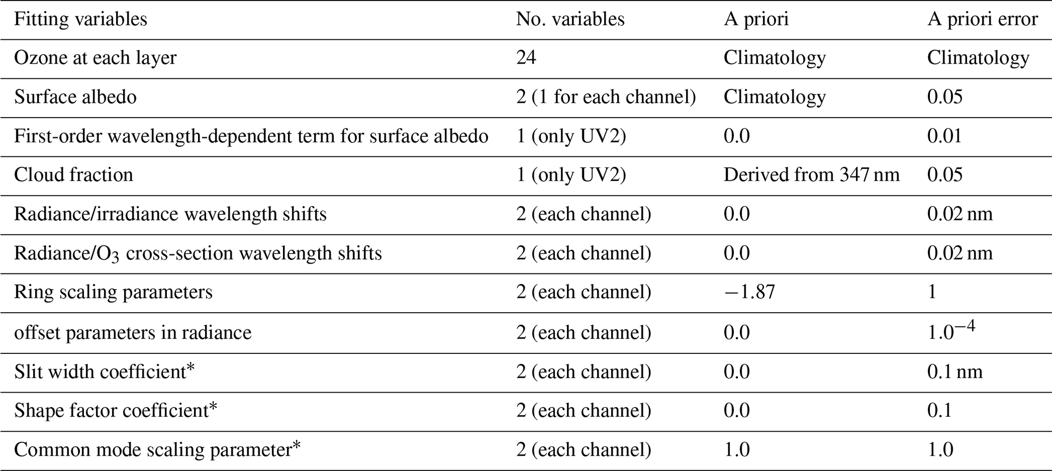
^* New variables incorporated into the OMPROFOZ v2 algorithm.

2.3 OMPROFOZ product

The previous version product was stored in the HDF-EOS5 format, but the NetCDF-4 format is applied to create the OMPROFOZ v2 product, similar to other collection 4 OMI data products. Also, it is written using the TEMPO output libraries so that it shares common data structures and metadata definitions with TEMPO data products.

The main product parameters are partial ozone columns at 24 layers, ∼ 2.5 km for each layer, from the surface to ∼ 65 km in Dobson units (DU, 1 DU $=\mathrm{2.69}\times {\mathrm{10}}^{\mathrm{16}}$ molecules cm⁻²). The 25-level vertical pressure grid is set initially at $P_i={\mathrm{2}}^{-i/\mathrm{2}}$ atm for i= 0, 23 and with the top of the atmosphere set for P₂₄. This pressure grid is then modified: the surface pressure and the thermal tropopause pressure are used to replace the level closest to each one, and tropospheric layers are distributed equally with logarithmic pressure. Correspondingly, the random noise error and solution error profiles are provided in terms of a square root of diagonal elements of random noise error covariance matrix S_n and solution error covariance matrix $\widehat{\mathbf{S}}$ that is directly estimated from the retrievals:

$$\begin{array}{}\text{(3)}& \begin{array}{rl}{\mathbf{S}}_n& ={\mathbf{GS}}_y{\mathbf{G}}^T,\widehat{\mathbf{S}}={\left({\mathbf{K}}^T{\mathbf{S}}_y^{-\mathrm{1}}\mathbf{K}+{\mathbf{S}}_{\mathrm{a}}^{-\mathrm{1}}\right)}^{-\mathrm{1}},\text{and}\\ & \mathbf{G}=\widehat{\mathbf{S}}{\mathbf{K}}^T{\mathbf{S}}_y^{-\mathrm{1}},\end{array}\end{array}$$

where G is the matrix of contribution functions. The smoothing error covariance S_s can be also directly estimated but is not provided in the output file. That is because it can be derived with the following relationship:

$$\begin{array}{}\text{(4)}& {\displaystyle }\widehat{\mathbf{S}}={\mathbf{S}}_{\mathrm{s}}+{\mathbf{S}}_n,\text{(5)}& {\displaystyle }{\mathbf{S}}_{\mathrm{s}}=\left(\mathbf{A}-\mathbf{I}\right){\mathbf{S}}_{\mathrm{a}}{\left(\mathbf{A}-\mathbf{I}\right)}^T,\end{array}$$

where I is the unit vector and A is the matrix of averaging kernels:

$$\begin{array}{}\text{(6)}& \begin{array}{rl}\mathbf{A}& ={\displaystyle \frac{\partial \mathit{X}}{\partial {\mathit{X}}_T}}={\left({\mathbf{K}}^T{\mathbf{S}}_y^{-\mathrm{1}}\mathbf{K}+{\mathbf{S}}_{\mathrm{a}}^{-\mathrm{1}}\right)}^{-\mathrm{1}}{\mathbf{K}}^T{\mathbf{S}}_y^{-\mathrm{1}}\mathbf{K}\\ & =\widehat{\mathbf{S}}{\mathbf{K}}^T{\mathbf{S}}_y^{-\mathrm{1}}\mathbf{K}=\mathbf{GK}.\end{array}\end{array}$$

A particular row of A describes how the retrieved profile in a particular layer is affected by changes in the true profile in all layers. It is a very useful variable to characterize the retrieval sensitivity and vertical resolution of the retrieved profile. The diagonal elements of A, known as degrees of freedom for signal (DFS), represent the number of useful independent pieces of information available at each layer from the measurement. To quantify the performance of the spectral fitting, the mean fitting residuals are calculated for each fitting window (UV1, UV2) in the form of the root mean square of spectral differences relative to the measured spectrum and the measured error as follows:

$$\begin{array}{}\text{(7)}& \begin{array}{rl}& \text{rms}=\sqrt{{\displaystyle \frac{\mathrm{1}}{N}}{\sum }_{\mathrm{1}}^N{\left(\left({\mathit{I}}_{\mathrm{m}}-{\mathit{I}}_{\mathrm{s}}\right)/{\mathit{I}}_{\mathrm{m}}\right)}^{\mathrm{2}}}\times \mathrm{100}\left(\mathit{\%}\right),\text{and}\\ & \text{RMSE}=\sqrt{{\displaystyle \frac{\mathrm{1}}{N}}{\sum }_{\mathrm{1}}^N{\left(\left({\mathit{I}}_{\mathrm{m}}-{\mathit{I}}_{\mathrm{s}}\right)/{\mathit{I}}_{\mathrm{e}}\right)}^{\mathrm{2}}},\end{array}\end{array}$$

where I_m, I_s, and I_e represent the measured spectrum, simulated spectrum, and measured errors, respectively, with N the number of the wavelengths in each window. The root mean square (rms) of fitting residuals needs to be better than 0.2 %–0.3 % in the Huggins band (310–340 nm) for reliable retrievals of tropospheric ozone (Munro et al., 1998). The root mean square (RMSE) describes both spectral fit quality and the stability of regularization. The ideal value of RMSE is 1. If RMSE ≪ 1, either the fitting is overfitted or the measurement errors are overestimated. On the other hand, if RMSE ≫ 1, either the fitting is underfitted or the measurement errors are underestimated.

3 Specification and verification of updated implementations

This section specifies new and improved updates made in the OMPROFOZ algorithm, listed in Table 3. The corresponding impacts on the spectral fit and ozone retrievals are verified. Note that the verification results of several implementations have already been presented in related papers indicated in the fourth column of Table 3, which is briefly described in this paper. The unpublished implementations are specifically described in this paper.

Table 3 List of updates to algorithm implementations.

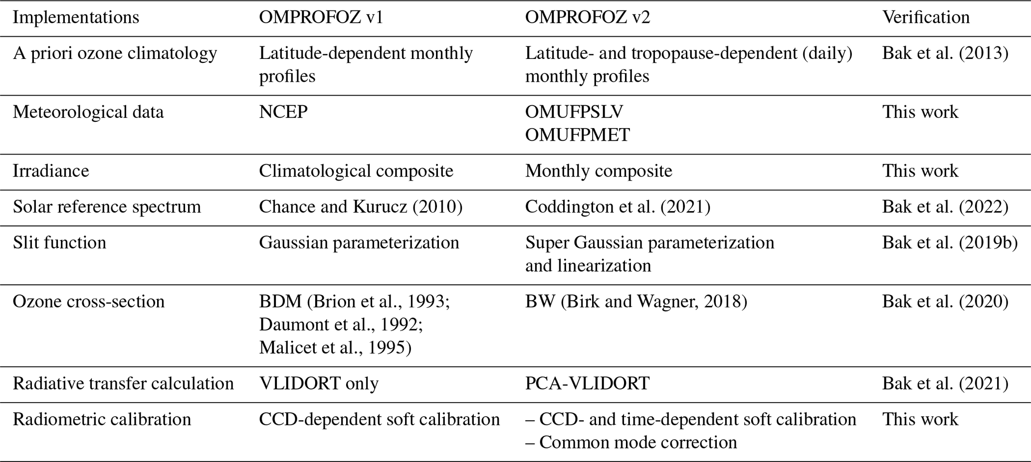
3.1 A priori ozone climatology

An OE-based ozone retrieval can be significantly affected by the quality of a priori data given insufficient measurement information. Therefore, the constraint can push the retrieval away from the actual state of the atmosphere toward a priori information, especially near the boundary layer or the tropopause where the vertical resolution of nadir satellite observations is inherently limited. In the v1 algorithm, the a priori ozone information was taken from McPeters et al. (2007) (abbreviated as LLM climatology) consisting of monthly average ozone profiles for every 10° latitude zone based on ozonesonde measurements in the troposphere and lower stratosphere and satellite measurements above. The v2 algorithm implements a tropopause-based (TB) ozone profile climatology from which a zonal monthly mean profile is vertically adjusted according to the tropopause height taken from the daily meteorological database described in Sect. 3.2. Applying the TB climatology as OMI a priori was thoroughly verified in Bak et al. (2013), who demonstrated improvements of OMI ozone profile retrievals in comparison with ozonesondes as well as in representing the sharp gradients of ozone vertical structures near the tropopause. Figure 2 compares tropospheric ozone retrievals on 1 February 2007 with a priori ozone constraints being taken from LLM and TB, respectively. The most noticeable difference is identified in the northern region of Europe where abnormally high concentrations are retrieved when LLM is used as a priori. This retrieval issue was also mentioned in comparing OMPROFOZ v1 with other satellite products, data assimilation, and chemical transport model calculation (Gaudel et al., 2018; Ziemke et al., 2014), showing large positive biases in tropospheric column ozone during high-latitude winter, but it has not been explained. It is clearly seen that the abnormal feature of the retrieved high ozone is closely correlated with the high LLM a priori (Fig. 2c) resulting from abnormally low tropopause pressure or high tropopause height (Fig. 2e). LLM can represent the typical vertical profiles whose ozonepause is located at ∼ 8 km over high latitudes during the winter. Therefore, with the presence of the abnormally high tropopause height, the lower-stratospheric layers of LLM profiles can be misrepresented as a priori in the upper-tropospheric ozone layers, which likely causes the large positive biases of ozone retrievals in the troposphere seen in OMPROFOZ v1. However, an ozone profile taken from the TB climatology is redistributed according to the daily tropopause, which becomes an ozonepause of TB profiles. In the subtropical region, LLM may also provide incorrect information in the presence of high tropopause height, but ozone retrievals are less affected, implying that OMI retrievals are less constrained by the a priori information in this case due to more measurement information, unlike in the northern high latitudes.

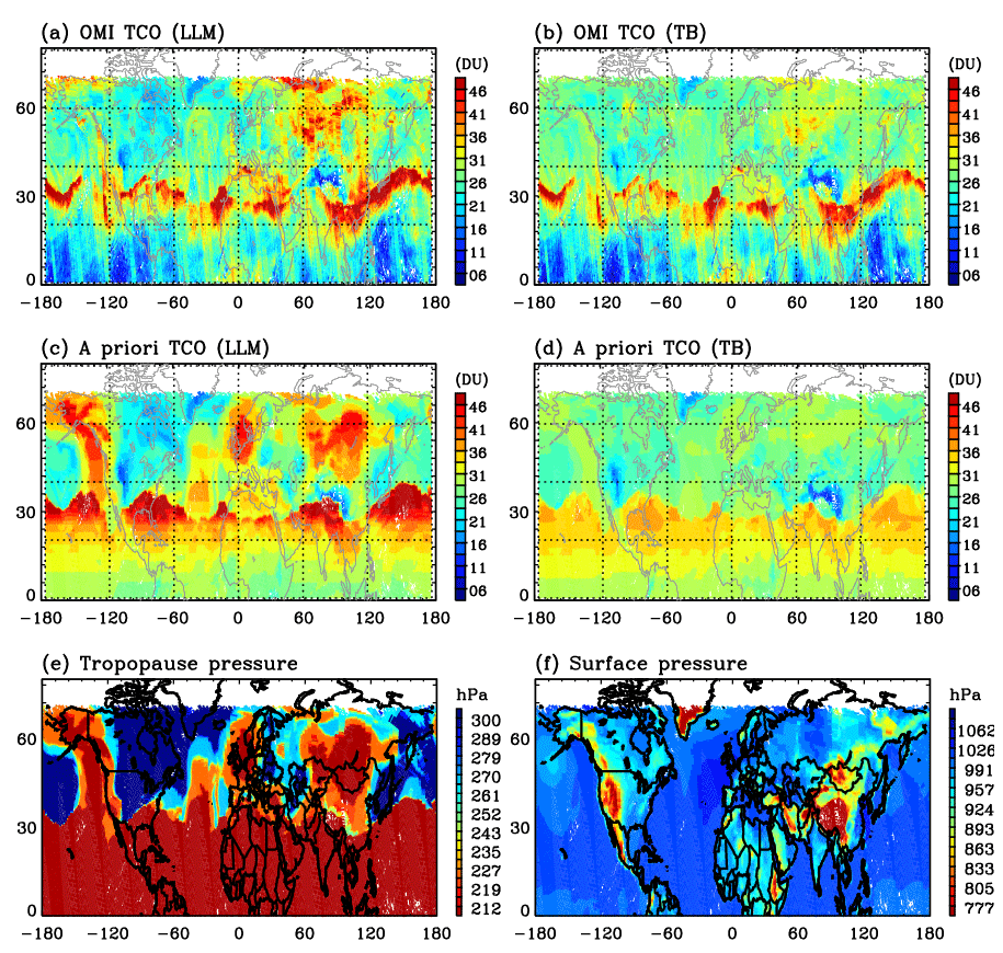
Figure 2 Comparison of (a, b) OMI tropospheric column ozone (TCO) and (c, d) the corresponding a priori TCO taken from monthly and zonal mean climatologies (LLM left, TB right), respectively, in the Northern Hemisphere on 1 February 2007. (e) Tropopause and (f) surface pressure fields are presented in the bottom panels. It is noted that the meteorological fields are commonly taken from the NCEP reanalysis data to see the impact of applying different a priori ozone data to the retrieval.

3.2 Meteorological data

As a forward model input, the surface pressure is required to define the bottom of the atmosphere, with the air temperature profile to account for the temperature dependence of the ozone absorption cross-section, especially in the Huggins band. The tropopause pressure is also required to be used as one of the retrieval vertical levels to separate stratospheric ozone from tropospheric ozone and determine the a priori ozone profile in the case of using the TB climatology. In v1, these meteorological variables were taken externally from National Centers for Environmental Prediction (NCEP) reanalysis data (http://www.cdc.noaa.gov/, last access: 12 March 2024), which provide 6-hourly (four times a day) global analyses on 2.5 ° × 2° grids with 17 vertical pressure levels below 10 hPa. These databases were pre-interpolated to 13:45 local solar time when OMI crosses the Equator and OMI's ground pixels using nearest-neighbor interpolation and then manually transmitted to OMI SIPS. However, the data transmission has been accidently halted since June 2011, and hence climatological monthly mean data have been used as a back-up in the data processing. To avoid this risk, the meteorological input is switched to the internal meteorological products, geo-collocated to the OMI UV-2 1-Orbit L2 Swath from the 2D Time-Averaged Single-Level Diagnostics (OMUFPSLV) and the GEOS-5 FP-IT 3D Time-Averaged Model-Layer Assimilated Data (OMUFPMET). We take the air temperatures given at 72 pressure levels above the center of the ground pixel from OMUFPMET as well as surface temperature, surface pressure, and thermal tropopause pressure at the center of the ground pixel from OMUFPSLV. The impact of switching meteorological input on the spectral fitting residuals is insignificant (not shown here), implying that the residuals might be absorbed by other state vectors. Figure 3 illustrates that ozone profile retrievals are changed by 2–3 DU, especially in the tropopause region due to changes in a priori ozone profiles in adjusting the climatological TB ozone profile around the daily tropopause height.

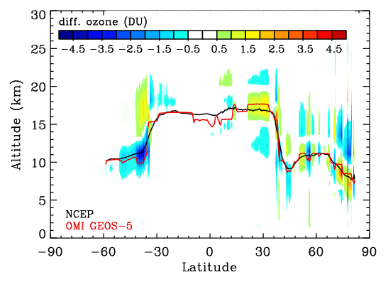
Figure 3 Differences of OMI ozone profile retrievals (DU) along the nadir view from the seventh orbit of measurements on 15 June 2006 due to switching the meteorological input from NCEP to OMI GEOS-5 (OMUFPSLV and OMUFPMET). The solid line represents the tropopause height from NCEP (black) and OMI GEOS-5 (red).

3.3 Ozone cross-section

The BDM cross-section measurements have been the standard input for retrieving ozone profiles using backscattered ultraviolet (BUV) measurements over the last decade (Liu et al., 2013, 2007; Orphal et al., 2016). In a related paper (Bak et al., 2020), the new BW ozone cross-section dataset was tested to check if there is room to improve our ozone profile retrievals, which made us switch the cross-section from BDM to BW in OMPROFOZ v2. As illustrated in Fig. 4 (top), the BW dataset provides improved temperature coverage from 193 to 293 K every 20 K over the BDM dataset given only at five temperatures above 218 K. Therefore, BW measurements were better parameterized as quadratic temperature-dependent coefficients with uncertainties of 0.25 %–2 %, whereas for BDM measurements fitting residuals of 2 %–20 % remain. Note that parameterized coefficients of cross-section measurements are typically applied in both column ozone and ozone profile retrievals for conveniently representing the temperature dependence of the cross-section spectrum. Bak et al. (2020) also showed a large impact of switching cross-sections on ozone profile retrievals when soft calibration is turned off. With soft calibration derived using consistent cross-sections, some of the systematic differences due to cross-sections can be greatly reduced; using BW can still improve the retrievals due to its better temperature dependence, but it does not cause the most impactful changes.

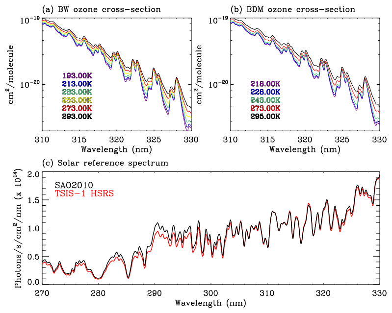
Figure 4 Comparisons of (a, b) ozone cross-sections and (c) the solar reference spectrum used in OMPROFOZ v1 and v2 algorithms. Note that the high-resolution solar reference spectrum is convolved with a Gaussian slit function of 0.4 nm FWHM (full width at half-maximum) resolution.

3.4 High-resolution solar reference spectrum

An accurate, high-resolution extraterrestrial solar reference spectrum is required for either wavelength calibration or slit function characterization. We decided to switch the solar reference spectrum from Chance and Kurucz (2010) to Coddington et al. (2021). Figure 4c illustrates radiometric discrepancies between the new solar reference called the TSIS-1 Hybrid Solar Reference Spectrum (HSRS) and the old solar reference called the SAO2010. A related paper evaluated the radiometric uncertainties of the new reference spectrum as below ∼ 1 %, whereas for SAO2010 they range from 5 % in the longer UV part to 15 % in the shorter UV part (Bak et al., 2022). Furthermore, they confirmed an opportunity to improve the spectral fitting of slit functions and hence the spectral fitting of ozone when using the TSIS-1 spectrum; the impact on ozone profile retrievals is 5 %–7 % in the troposphere.

3.5 Solar irradiance spectrum

OMI makes solar irradiance measurements near the Northern Hemisphere terminator of an orbit once per day, which are required to calculate top-of-atmosphere reflectance and to estimate an on-orbit slit function in ozone profile retrievals. In order to reduce the short-term noise of individual measurements, the earlier algorithm implemented the use of climatological solar spectra derived from 3 years of daily OMI L1b products (2005–2007). In the newer algorithm, collection 4 irradiance spectra are tabled as a monthly average to improve short-term noise and address seasonal variations of instrument characteristics that are common in both radiance and irradiance measurements. Figures 5 and 6 compare irradiance measurements averaged over July for each year from collection 3 and collection 4, respectively. Collection 3 shows significant short-term noise in daily measurements in the UV2 range of around 3 %–5 % and also systematically decreasing patterns of monthly irradiance spectra from −10 % in the UV1 range to −6 % in the UV2 range over the mission. Collection 4 provides much improved irradiance spectra with respect to both degradation and noise errors. In addition, OMI random noise errors in the monthly average spectra are compared. Collection 4 ranges from 0.02 % in the UV1 to 0.04 % in the UV2 consistently over the mission. However, collection 3 shows somewhat different features in the UV2 range, like more wavelength dependence and a systematic drift as of 2008–2009. Figure 7 shows the impact of switching the OMI L1b product from collection 3 to 4 on fitting residuals resulting from ozone profile retrievals on 16 July 2020; the average fitting residuals are plotted as a histogram for each fitting window. In this experiment, the v2 implementations are identically applied without radiometric corrections (soft calibration and common mode correction are turned off). In addition, the impact of using monthly and daily irradiance is investigated. As shown, fitting residuals are noticeably improved in both fitting windows due to switching from collection 3 to 4. This experiment illustrates that monthly irradiances should be used instead of daily measurements when using the collection 3 product. In comparison, the corresponding impact on fitting residuals with the collection 4 product is not very significant due to improvements of short-term noise errors in daily irradiance measurements, but the number of retrievals with smaller fitting residuals increases in the UV2 band.

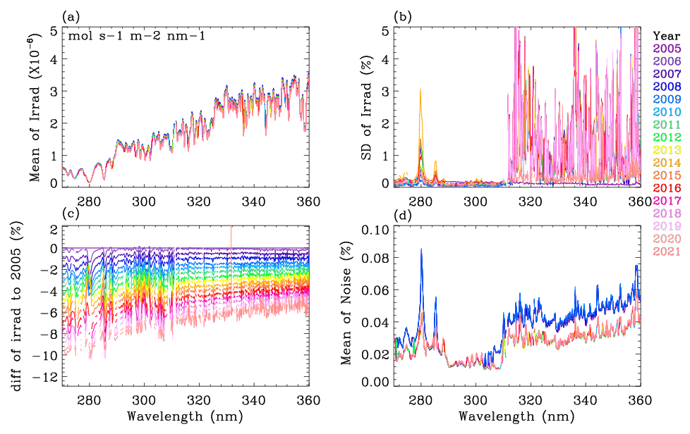
Figure 5 (a) Monthly mean irradiance spectra of the OMI collection 3 product in July from 2005 to 2021 at the 10th cross-track position for the UV-1 band and 20th cross-track position for the UV-2 band without co-adding. (b) Corresponding standard deviations of the monthly mean irradiances, (c) biases of the mean irradiances relative to 2005, and (d) monthly mean random noise errors.

Figure 6 Same as Fig. 5, but for the OMI collection 4 irradiance product.

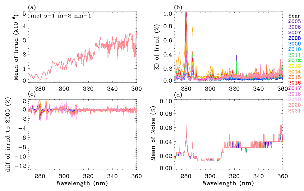
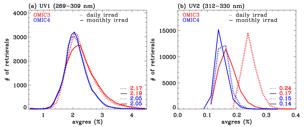
Figure 7 Histograms of average fitting residuals from OMI collection 3 (red) and 4 (blue) L1b products on 15 July 2020 in (a) UV1 and (b) UV2 ranges, respectively. In order to make a fair comparison, this experiment limits OMI measurements to the western side of the swath to avoid using row-anomaly cross-track pixels and empirical recalibration is not applied. Fitting residuals are evaluated with both daily (dashed) and monthly mean (solid) OMI irradiance measurements. The median values of average fitting residuals are presented in the legend.

3.6 Instrument spectral response function (ISRF) parameterization and linearization

OMI ISRFs were previously parameterized as a standard Gaussian by fitting the slit width (w) from OMI solar irradiances separately for each channel and each cross-track position. In the updated implementation, one more parameter, the shape factor (k), is added to parameterize ISRFs as a super Gaussian $\left(S\left(\mathrm{\Delta }\mathit{\lambda }\right)=\exp \left[-{\left|\frac{\mathrm{\Delta }\mathit{\lambda }}{w}\right|}^k\right]\right)$. However, slit functions in radiance could deviate from those derived from solar spectra due to the sensitivity to scene heterogeneity, differences in stray light between radiance and irradiance, and intra-orbit instrumental changes. These might cause some spectral structures in the radiance fitting. Therefore, the v2 algorithm treats these spectral errors as pseudo-absorbers (PAs), which is derived as $\frac{\partial I}{\partial p}$ (p=w or k) through the slit function linearization. As specified in Table 2, these PAs are iteratively adjusted with a zero-order scaling parameter. These PA coefficients are weakly correlated with ozone variables, except for the UV2 shape factor coefficient (Δk) and tropospheric ozone (0.2–0.3). The description and evaluation of this implementation for OMI ozone profile retrievals are detailed in a related paper (Bak et al., 2019b).

3.7 Radiative transfer calculation

The radiative transfer (RT) model is needed for calculating the forward model component such as top-of-the-atmosphere radiances and Jacobians of radiances with respect to the atmospheric and surface parameters. The radiance calculation is made for a Rayleigh atmosphere (no aerosols) with Lambertian reflectance assumed for the surface and for clouds. The independent pixel approximation (IPA) is employed to treat partial clouds by assuming a cloud reflectivity of 80 %:

$$I=I\left(R_{\mathrm{sfc}},P_{\mathrm{sfc}}\right)(\mathrm{1}-f_{\mathrm{c}})+I\left(R_{\mathrm{cloud}},P_{\mathrm{cloud}}\right)f_{\mathrm{c}},$$

where R and P represent reflectivity and pressure at bottom level (surface or cloud) with f_c as an effective cloud fraction. According to the Nyquist criterion (Goldman, 1953), individual spectra need to be simulated at grid spacings finer than a minimum of 2 pixels (4 pixels in practice) per spectral resolution. To reduce the computational burden, a few wavelengths are effectively selected (λ_e) for running the RT model and then interpolated to regular high-resolution grids (λ_h) with the radiance adjustment for errors caused by the spectral resolutions as follows:

$$\begin{array}{}\text{(8)}& \begin{array}{rl}I\left({\mathit{\lambda }}_{\mathrm{h}}\right)& =I\left({\mathit{\lambda }}_{\mathrm{e}}\right)+{\sum }_{l=\mathrm{1}}^N{\displaystyle \frac{\partial I\left({\mathit{\lambda }}_{\mathrm{e}}\right)}{\partial {\mathrm{\Delta }}_l^{\mathrm{gas}}}}\left({\mathrm{\Delta }}_l^{\mathrm{gas}}\left({\mathit{\lambda }}_{\mathrm{h}}\right)-{\mathrm{\Delta }}_l^{\mathrm{gas}}\left({\mathit{\lambda }}_{\mathrm{e}}\right)\right)\\ & +{\displaystyle \frac{\partial I\left({\mathit{\lambda }}_{\mathrm{e}}\right)}{\partial {\mathrm{\Delta }}_l^{\mathrm{ray}}}}\left({\mathrm{\Delta }}_l^{\mathrm{ray}}\left({\mathit{\lambda }}_{\mathrm{h}}\right)-{\mathrm{\Delta }}_l^{\mathrm{ray}}\left({\mathit{\lambda }}_{\mathrm{e}}\right)\right),\end{array}\end{array}$$

where $\frac{\partial I}{\partial {\mathrm{\Delta }}_l}$ represents Jacobians with respect to optical properties at layers l (l=1 to N). In the v2 forward model, both λ_c and λ_h are set to be finer than intervals previously used as noted in Table 4 where the implementation details between v1 and v2 forward models are compared. To accelerate forward model calculations, the RT model has been switched from the earlier version 2.4 of VLIDORT to a newer PCA-based VLIDORT model (version 2.8). Formerly, multiple scattering (MS) calculations were performed at individual wavelengths, whereas in the newer model MS calculations are carried out only for a few EOF-derived optical states which are developed from spectrally binned sets of inherent optical properties that possess some redundancy. In both these VLIDORT-based forward models, the polarization is not accounted for in the direct RT simulation of the entire spectrum; instead, polarization correction is applied to speed up the RT. In the earlier forward model, vector calculations are additionally executed at 14 wavelengths to establish 14 scalar vs. vector intensity differences which are then interpolated to all other wavelengths. However, residual polarization errors remain, along with other forward model errors arising from the use of a low number of discrete ordinates (4 streams in each polar hemisphere) and relatively coarse vertical layerings (∼ 2.5 km thick). The newer forward model reduces the number of half-space discrete ordinate streams from 4 to 2, and this increases the speed by a factor of ∼ 2. To compensate for the resulting increase in RT approximation errors, a correction based on a lookup table (LUT) is performed; this corrects for the differences in RT variables due to the number of discrete ordinates (2 vs. 6) and number of layers (24 vs. 72) as well as correcting for the neglect of polarization. As described in a related paper, these updates improve the retrieval speed by a factor of ∼ 3.3 as well as the retrieval accuracy (Bak et al., 2021). Note that the ring simulation remains unchanged from the v1 algorithm; the spectral structure of the ring signal is externally simulated with the iterative fitting of amplitude of the ring spectrum and then subtracted from the measured spectral reflectance (Liu et al., 2010).

Table 4 Comparison of implementation details for forward model simulation.

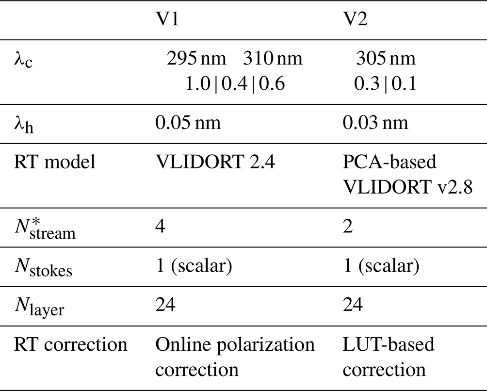
^* The N_stream is the number of discrete ordinate streams in the half-space.

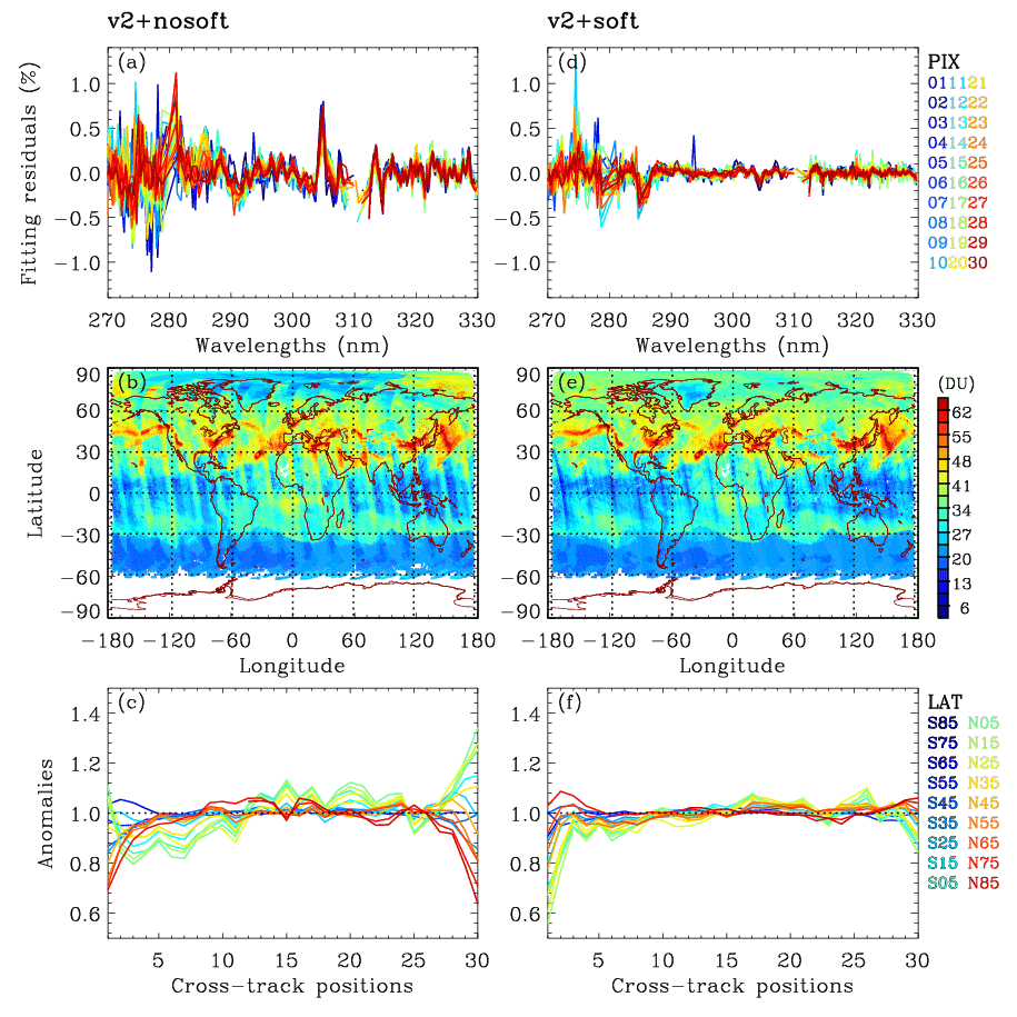
Figure 8 (a, d) Spectral fitting residuals (%) averaged in the latitude of 60° S and 60° N from OMI measurements on 15 June 2006, (b, e) the global distribution of tropospheric column ozone (TCO, DU), and (c, f) anomalies of TCO as a function of 18 latitude bands. Left and right panels are for without and with soft calibration, respectively.

3.8 Soft calibration

The left panels of Fig. 8 show (a) the spectral fitting residuals averaged in the latitude band of 60° S to 60° N, (b) tropospheric column ozone (TCO) distribution, and (c) cross-track-dependent stripe errors of TCOs where the OMI collection 4 L1b product is applied without any radiometric corrections. As shown, quite persistent residuals remain of up to ∼ 1.0 % in the UV1 range and of up to 0.3 % in the UV2 range. The TCO distribution shows the along-track stripes that are commonly found in OMI trace gas products (e.g., Kroon et al., 2011; Lamsal et al., 2021; Wang et al., 2016). The cross-track-dependent stripes of TCO are evaluated for 18 bands of latitude, as anomalies in the ratio of each cross-track column to the average column taken within cross-track positions 5–25 (1-based). The amplitude of anomalies is within ±10 % at nadir pixels but reaches 40 % at off-nadir pixels, with some dependency on latitudes. However, stratospheric column ozone (SCO) retrievals are almost free of stripe errors (not shown here). To reduce the striping, a soft calibration was applied to OMI radiances in OMPROFOZ v1. The soft spectra are derived as a systematic component of differences between measured and simulated radiances at tropical clear-sky pixels in summer where the forward model calculations are more accurate to attribute the residuals to measurement biases. The soft spectra are re-derived for the OMI collection 4 L1b product using the v2 forward model calculations (Sect. 3.7). The ozone profile input is prepared from 10° zonal averages of daily MLS measurements above 215 hPa and climatological ozone profiles below 215 hPa taken from McPeters and Labow (2012). In order to account for the daily variability, the climatological profile is scaled to match the total ozone value taken from 10° zonal averages of the level 3 OMI TOMS-like total ozone product (OMTO3d). To smooth out the impact of daily ozone variabilities, 1-week measurements during 11–17 July over the tropics 20° S–20° N are used in deriving the soft spectra after screening out outliers of extreme viewing geometries (SZA > 60°), cloudy pixels (f_c> 0.2), bright surfaces (A_sfc> 0.1), and aerosol-contaminated pixels (aerosol index > 5), as well as abnormally large values of average residuals (UV1 > 8, UV2 > 3). Note that the threshold value of filtering out aerosol pixels needs to be relaxed due to the overestimation errors of aerosol index at initial iteration. Figure 9 displays the cross-track-dependent soft spectrum for the case of July 2005 when instrument degradation is negligible and row-anomaly damage has not occurred. It illustrates the existence of systematic residuals between measured and simulated radiances within 2 % in UV2 and mostly from −7 % to 3 % in the UV1, except for some spikes. The right panels of Fig. 8 demonstrate how soft calibration works for improving ozone retrievals in comparison to the left panels where soft calibration is tuned off. It is clearly shown that the systematic spikes are mostly eliminated and cross-track-dependent stripes are globally reduced even up to high latitudes. In particular, the “anomalies” are reduced to within 0.1 %, except at the first cross-track pixels. This calibration has been applied independent of time and latitude in the v1 algorithm. To account for OMI degradation errors, the v2 soft spectra are developed for every year. As an example, the yearly soft spectra are displayed at several cross-track positions in Fig. 10. There is noticeable yearly variation in the UV1 band, typically within 2 %–3 % over 17 years. The most significant degradation features are found at the first cross-track pixel in the UV1 band, with a relative change of 5 % or more. For cross-track positions 13, 18, and 22, correction spectra cannot be derived for most of the time periods after 2008 due to the occurrence of a serious row anomaly. Although correction can be derived for cross-track position 13 during 2020, it is significantly different from those before 2008, indicating that it is still affected by the row anomaly. The yearly variation in the UV2 band is much smaller and can be clearly identified below ∼ 315 nm to be within 1 %. However, it could have a significant impact on ozone profile retrievals because the spectral fit residuals need to be smaller than 0.2 %–0.3 % in the Huggins band for reliable retrieval quality of tropospheric ozone (Munro et al., 1998).

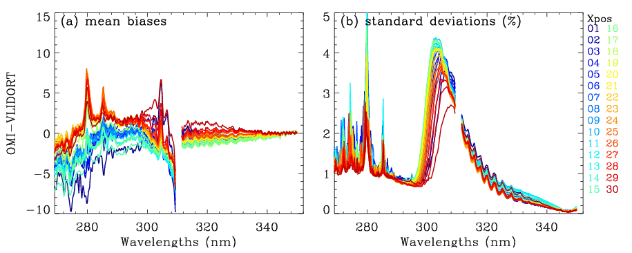
Figure 9 (a) Soft calibration spectra derived for collection 4 OMI L1b products on 11–17 July 2005, representing the systematic biases between the measured and simulated spectrum. (b) The standard deviations of the systematic biases, representing the uncertainties of soft calibration spectra.

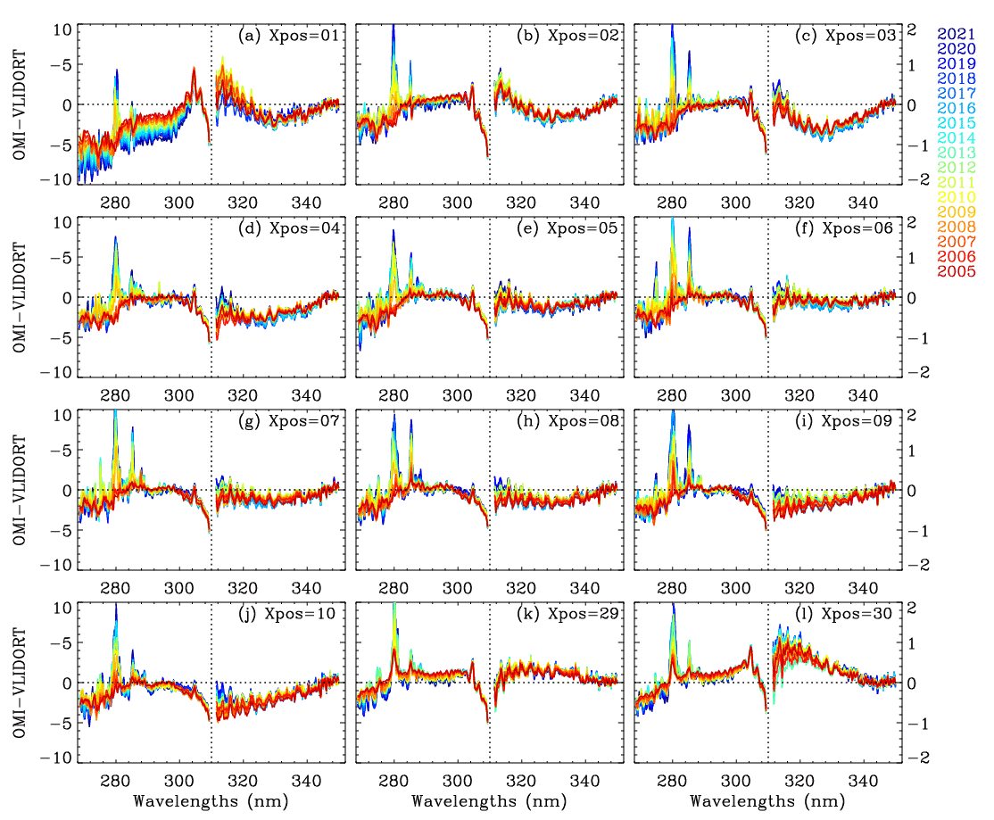
Figure 10 Yearly dependent soft calibration spectra from 2005 to 2021 at several cross-track positions (Xpos, UV1-based) which have not been affected by row anomalies over the mission. Note that the UV1 and UV2 bands are plotted with different y-axis ranges (left y axis for UV1 and right y axis for UV2) for better visualization.

3.9 Common mode correction

As compared in Fig. 11 (left and middle panels), the soft calibration is less effective in eliminating the systematic residuals at high solar zenith angles, especially in the UV2 band where the spectral residuals vary from 0.1 % at lower SZAs to 0.4 % at higher SZAs. This implies the existence of a spectral dependence of the radiometric calibration and detector sensitivity to the signal represented by solar zenith angle, which is not accounted for in the soft calibration dependent only on CCD dimension. Therefore, common mode correction (CMC) is newly implemented in OMPROFOZ v2 to correct the remaining radiometric errors. The common mode spectrum of the fitting residuals is physically treated as a pseudo-absorber, along with a scaling coefficient that is iteratively fitted in each of the UV1 and UV2 windows. Therefore, the scene-dependent radiometric errors could be partly accounted for. This kind of correction is originally used in the spectral fitting process where a common mode residual could be calculated online for each orbit of measurement. However, additional online calculation is not practical for the time-consuming optimal-estimation-based ozone profile retrieval process. Therefore, we derive time-independent common mode spectra by averaging 3 d of fitting residuals (13–15 July 2005) over five solar zenith angle regimes $[\mathrm{0}-\mathrm{40}\mathit{°},\mathrm{40}-\mathrm{60}\mathit{°},\mathrm{60}-\mathrm{70}\mathit{°},\mathrm{70}-\mathrm{80}\mathit{°},\mathrm{80}-\mathrm{85}\mathit{°}]$ for each cross-track position. As demonstrated in Fig. 11 (right panel), the applied common mode spectrum is likely to absorb the remaining spectral errors and hence the fitting accuracy is globally improved. For example, the systematic features are clearly reduced above 285 nm in the UV1 window, but the noisy features are still not well fitted below 285 nm. In the UV2 band, applying CMC reduces the dependence of fitting residuals on both solar zenith angle and cross-track pixels, and hence the remaining residuals are globally less than 0.1 % at most wavelengths. As shown in Fig. 12, striping patterns of tropospheric ozone retrievals could be reduced due to improvements of retrievals at the first cross-track pixels in the tropics where soft calibration deepens anomalies (Fig. 8f). Comparisons with OMPROFOZ v1 retrievals (Fig. 12d–f) demonstrate that the OMPROFOZ v2 product provides global information on tropospheric column ozone with smaller retrieval biases due to radiometric calibration errors and more consistent data quality with respect to different viewing geometries and latitude.

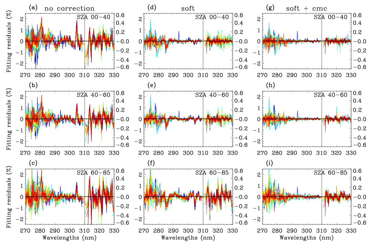
Figure 11 Comparison of spectral fitting residuals (%) averaged for three solar zenith angle regimes (00–40, 40–60, and 60–85°) from OMI measurements on 15 June 2005, with different radiometric calibration settings: (a, b, c) all radiometric correction turned off, (d, e, f) soft calibration turned on, (g, h, i) soft calibration and common model correction turned on. Note that the residuals are plotted in a different y-axis range below (left y axis) and above (right y axis) 310 nm, respectively.

4 Validation with ozonesonde measurements

Comparisons against ozonesonde measurements are performed to highlight improvements of data quality and long-term consistency of OMPROFOZ v2 over OMPROFOZ v1. Ozonesonde measurements are obtained from three sites over central Europe during the period of 2005 to 2020, listed in Table 5. Balloon-borne ozone profiles are regularly measured two to three times per week at these sites located close to each other. The coincidence criteria used to pair OMI and ozonesonde measurements are within 100 km and 6 h, and then the closest pair is selected after screening out row-anomaly-flagged pairs. For comparison, individual ozonesonde soundings are converted from mPa into DU and then interpolated at OMI vertical grids, but without adjusting the vertical resolution to address the total errors of OMI retrievals including smoothing errors. The relative difference is calculated as (OMI-ozonesonde) $/$ ozonesonde × 100 %. Extreme values that are beyond the mean by 3σ are dropped in estimating the comparison statistics. The comparison statistics of tropospheric column ozone between OMI and ozonesondes are summarized in Table 5 for each station. Overall, the mean biases (MBs) are within ±3 DU (5 %–10 %) with standard deviations (SDs) of 5.5 DU (15 %) and correlation coefficients of 0.81–0.85 for the updated product. These comparison statistics represent improvements over those derived for the existing product. Figure 13 shows comparisons of ozone profiles between OMI and ozonesondes during the periods before and after the row anomaly (RA), respectively. The pre-RA period is set to be from the beginning of the mission through 2008 when the row anomaly affects the data in a few rows, and the post-RA period is after that. Both v1 and v2 profiles are positively biased relative to ozonesonde measurements. The MBs of profile differences are less than 20 % over the layers when OMPROFOZ v2 profiles are compared during the pre-RA period. On the other hand, MBs of OMPROFOZ v1 are largely skewed by ∼ 45 % in the tropopause region. The comparison also confirms significant improvements of OMPROFOZ v2 retrievals, with the reduction of SDs by ∼ 40 % around the tropopause. These improvements are achieved mainly due to implementing TB ozone profile climatology, which could better represent the profile shape in the UTLS as mentioned in Sect. 3.1. Comparison statistics between OMPROFOZ v2 and ozonesonde profiles are generally consistent before and after the RA occurrence in spite of the inconsistent sampling resulting from the occurrence of RA so that only about half of the OMI measurements remain valid, mostly west of nadir during the post-RA period. However, OMPROFOZ v1 profiles are shown to be much more affected by temporal changes in OMI instrumental stability, especially in the lower atmosphere.

Table 5 List of ozonesonde stations¹ and comparison statistics² of the tropospheric column ozone (900–200 hPa) between OMPROFOZ and ozonesondes.

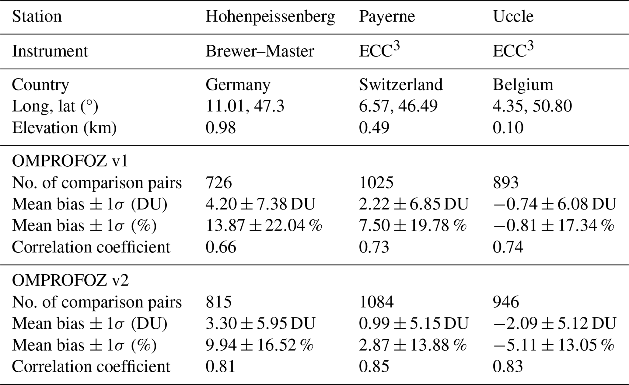
¹ All data are downloaded from the World Ozone and Ultraviolet Data Center (WOUDC) via https://woudc.org/ (last access: 12 March 2024).
² The number of comparison pairs between OMI and ozonesonde during the period 2005 to 2020. Mean biases and 1σ standard deviations are in both DU (Dobson units) and percent from (OMI–ozonesonde) $\times \mathrm{100}/$ ozonesonde.
³ Electrochemical concentration cell (ECC).

The rest of this section is concentrated on assessing the consistency of tropospheric ozone retrieval quality with respect to temporal changes. For this comparison, tropospheric ozone columns (TCOs) are integrated over the troposphere between 200 and 900 hPa from ozone profiles to avoid the impact of different meteorological inputs used in v1 and v2 retrievals. In order to check the seasonal changes in retrieval quality, comparison statistics of tropospheric ozone between OMI and ozonesondes are derived for each month during the pre-RA period. The seasonal changes in retrieval quality could be mainly related to the solar zenith angle dependency of OMI measurement sensitivity to lower-tropospheric ozone, which also causes the inconsistency of retrieval quality between lower and higher latitudes. As shown in Fig. 14a, monthly biases of OMI TCO are minimized below ∼ 2 DU from June to October when the solar zenith angles are relatively small, commonly for OMPROFOZ v1 and v2. However, the mean biases of OMPROFOZ v1 increase up to ∼ 6–9 DU during January–March, while OMPROFOZ v2 shows a moderate change in monthly biases from winter to summer, with smaller SDs of TCO differences by ∼ 3–4 DU during December–March (Fig. 14b).

In order to check the long-term stability, TCO differences are averaged into four seasons for each year from 2005 to 2020 in Fig. 14c and d. The existence of a long-term drift is clear with MBs of OMPROFOZ v1 TCO decreasing from ∼ 4.35 DU before 2008 to ∼ 0.05 DU after 2015. This temporal drift is largely corrected in OMPROFOZ v2 retrievals and the standard deviations of TCO differences are generally reduced over the entire period. In addition, OMPROFOZ v1 shows more spikes in both MBs and SDs than OMPROFOZ v2, especially during the period of 2011 to 2015 when the RA dynamically expands. Those spikes could be attributed to row-anomaly-contaminated retrievals unscreened with the row-anomaly flags taken from the OMI collection 3 L1b product. The related improvements in OMPROFOZ v2 retrievals are contributed by applying stricter flags taken from the OMUANC product.

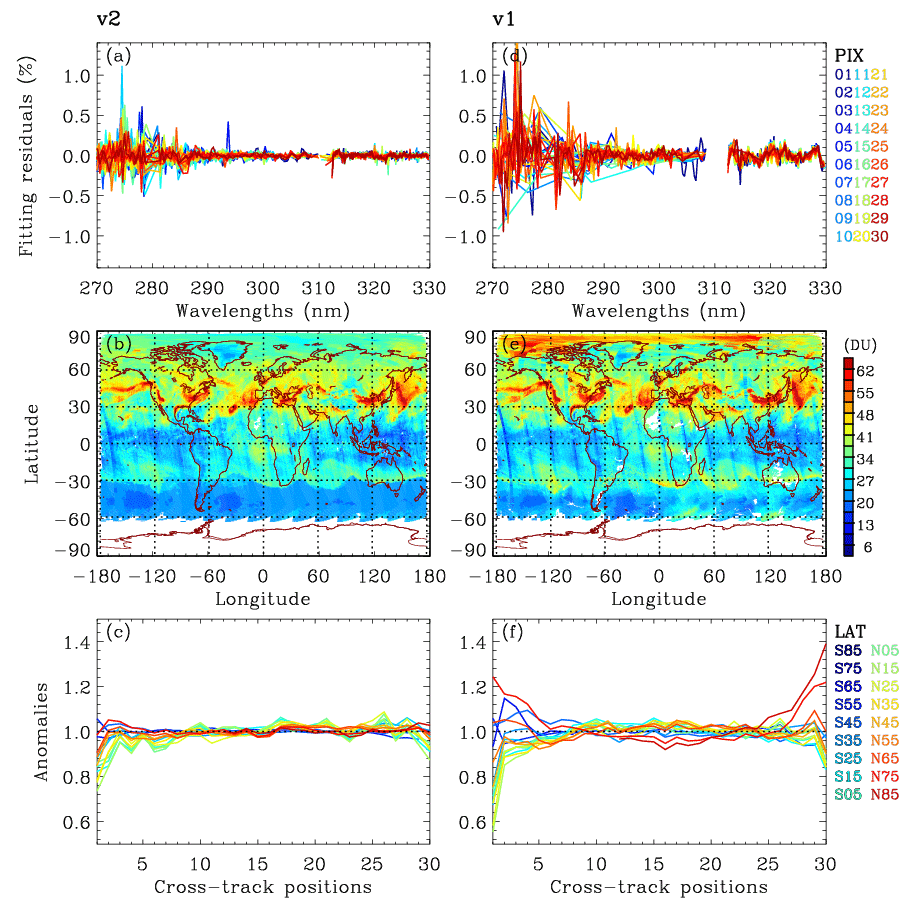
Figure 12 Same as Fig. 8, but for V2 (OMI collection 4 product with the final v2 algorithm) and V1 (OMI collection 3 with the v1 algorithm).

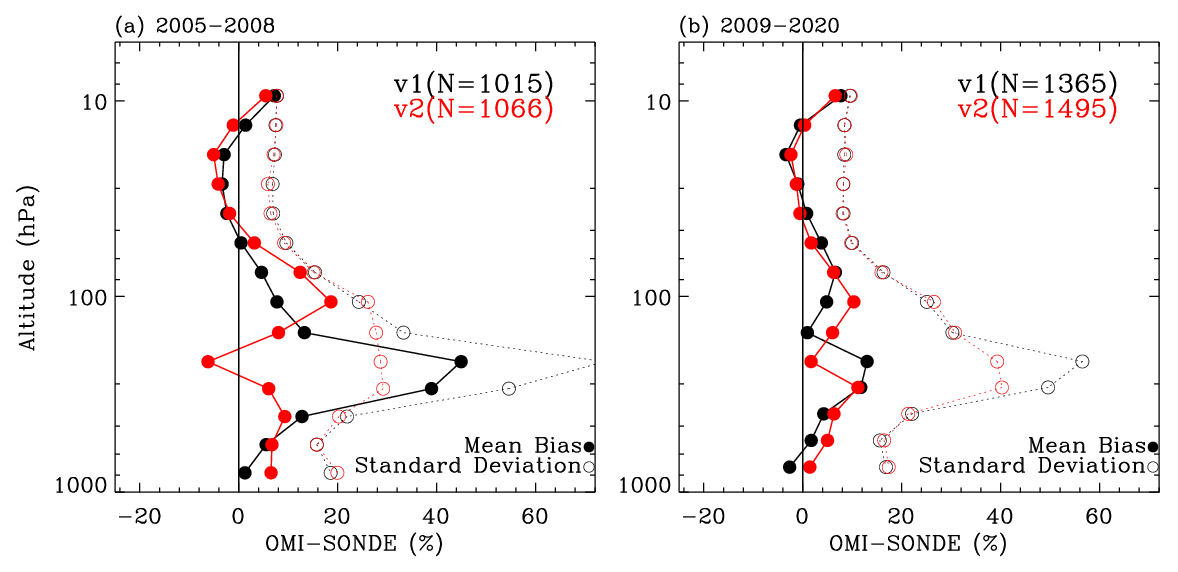
Figure 13 Comparisons of ozone profiles between OMI and ozonesonde during (a) pre-row anomaly and (b) post-row anomaly periods, respectively. OMI retrievals are qualified with RMSE < 3, rms < 2 %, and cloud fraction less than 0.6. The number of coincident pairs (N) is given in legend.

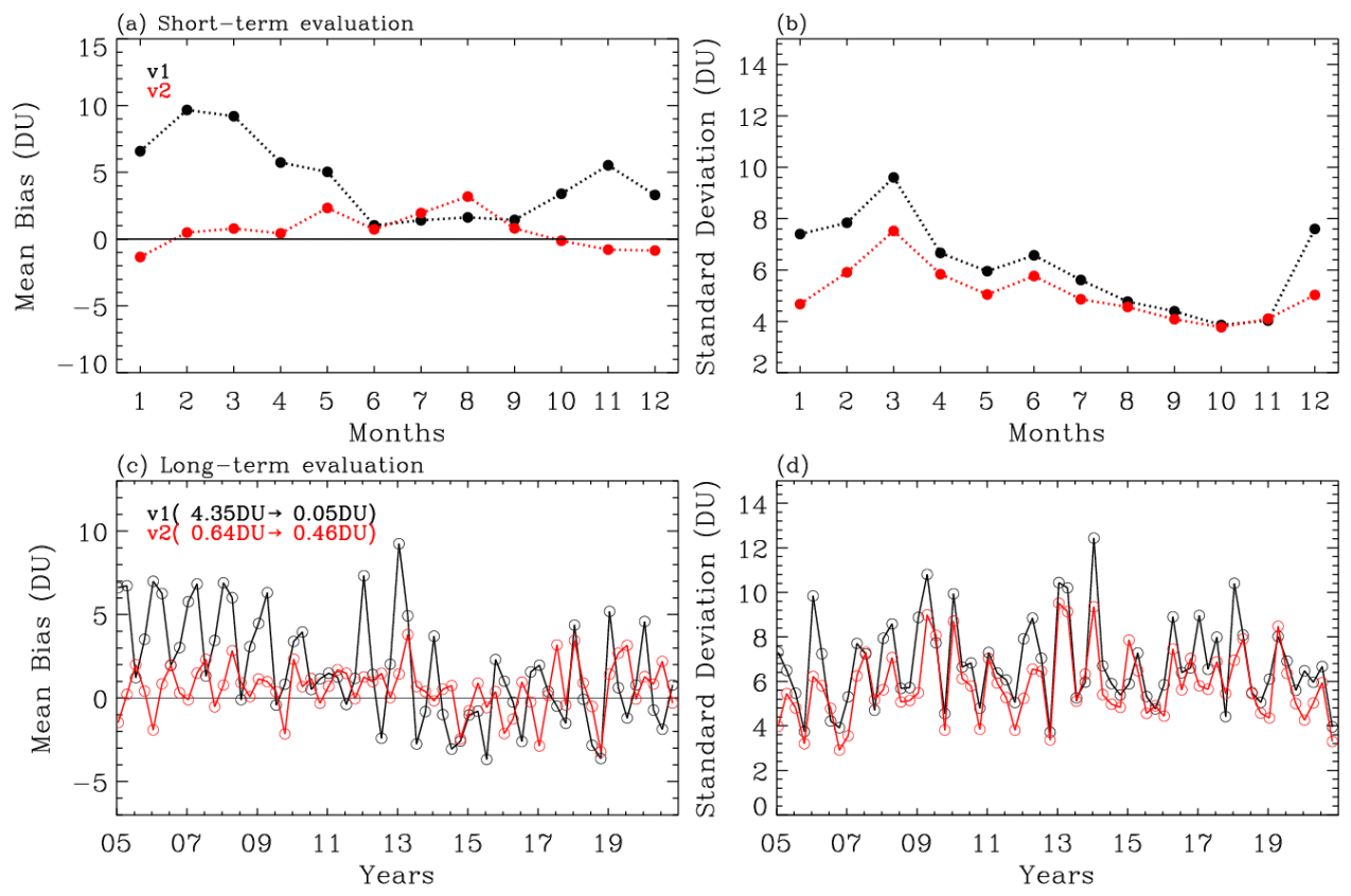
Figure 14 (a) Monthly mean and (b) corresponding standard deviations for differences in tropospheric column ozone (TCO, 200–900 hPa) between OMI and ozonesondes during the period of 2005 to 2008. Panels (c) and (d) are the same as panels (a) and (b), but for seasonal differences in TCO from 2005 to 2020. The legend in panel (c) represents the overall mean for the periods of 2005–2008 and 2015–2020.

5 Summary and conclusion

The Smithsonian Astrophysical Observatory (SAO) ozone profile retrieval algorithm has been run in NASA's Science Investigator-led Processing System (SIPS) to create the Ozone Monitoring Instrument (OMI) ozone profile (OMPROFOZ) research product, which has not been updated since its initial data release. In this paper, we introduce algorithmic updates for reprocessing the OMPROFOZ product to enhance the retrieval accuracy and to ensure long-term consistency. This second version will be released at GES-DISC, while the first version will remain archived at AVDC. One of the major changes is to switch the L1b data from collection 3 to collection 4 for both radiance and irradiance as well as the accompanying auxiliary datasets. We also changed several geophysical and spectroscopic inputs including meteorological data, ozone profile climatology, the high-resolution solar reference spectrum, and the ozone absorption cross-section dataset. Implementations of forward model calculations and measurement calibrations are improved. The v2 forward model employs a faster VLIDORT model based on principal component analysis (PCA), along with the LUT-based correction which speeds up the online radiative transfer model calculation while corrections to the approximation produce improved accuracy. The resulting speed-up allows OMI native measurements to be processed for OMPROFOZ, with data resolution of 48 × 26 km² at nadir. Note that to meet the computational cost, the previous data were processed after co-adding OMI measurements at the spatial resolution of 48 × 52 km². To better represent the shape of OMI slit functions, the slit width and shape factor are parameterized from OMI irradiances, assuming a super Gaussian instead of a normal Gaussian. Moreover, the effects of slit function differences between radiance and irradiance on ozone retrievals are accounted for as pseudo-absorbers in the iterative fit process. The OMI irradiance measurements are included via a monthly average instead of a 3-year climatological mean to cancel out the temporally varying calibration parameters commonly existing in radiance and irradiance measurements. The empirical soft calibration spectra are re-derived annually to be consistent with the updated implementations to remove the systematic differences between measured and simulated radiances. Common mode correction spectra are derived from remaining residual spectra after soft calibration with the dependency on solar zenith angle. The common mode is included as a pseudo-absorber in the iterative fit process, which helps to smooth out the discrepancies of ozone retrieval accuracy between lower and higher solar zenith angles and between nadir and off-nadir pixels.

To verify improvements of data quality, both v1 and v2 ozone profiles are evaluated against ozonesonde measurements collected from three stations over central Europe during the period of 2005–2020. Overall, the consistency of the tropospheric columns between OMI and ozonesondes is improved by 0.1–0.15 in correlation coefficients and by 3 %–6 % in standard deviations of individual differences (Table 5). It is clearly shown that ozone profile retrievals are greatly improved in the troposphere, especially around the tropopause, with the reduction of mean biases by ∼ 25 % during the pre-RA season (Fig. 13). The standard deviations of mean biases are also improved by ∼ 40 % and ∼ 20 % before and after the RA occurrence. The comparison with ozonesondes also confirms that the temporal consistency of tropospheric ozone quality is improved (Fig. 14). The seasonal change in data quality from summer to winter is predominant in OMI tropospheric ozone with the v1 data processing. However, OMPROFOZ v2 data quality shows much better consistency, with the seasonal changes in retrieval biases within ∼ 2–3 DU. Above all, we confirm that the OMI long-term degradation is better accounted for in the v2 data processing, along with switching OMI L1b data from collection 3 to collection 4 and updating implementation details. In OMPROFOZ v1, mean biases of tropospheric ozone relative to ozonesondes show a drift in errors from 4.35 to 0.05 DU before and after the RA occurrence, which are greatly reduced to within ±0.5 DU for both periods in OMPROFOZ v2.

This new algorithm has been delivered to the NASA OMI SIPS for operational processing and the reprocessing of the entire mission is in progress. The OMPROFOZ v2 product will be distributed via the NASA GES DISC in 2024. In the follow-up paper to this work, the reprocessed OMI collection 4 ozone profile dataset will be thoroughly evaluated against a comprehensive dataset of ozonesonde soundings and MLS stratospheric ozone profiles for establishing geophysical validation results and for ensuring the long-term consistency of OMI ozone profile product data quality.