An improved BRDF hotspot model and its use in VLIDORT for studying the impact of atmospheric scattering on hotspot directional signatures in the atmosphere

The term “hotspot” refers to the sharp increase in the reflectance occurring when incident (solar) and reflected (viewing) directions almost coincide in the backscatter direction. The accurate simulation of hotspot directional signatures is important for many remote sensing applications. The RossThick–LiSparse–Reciprocal (RTLSR) bidirectional reflectance distribution function (BRDF) model is widely used in radiative transfer simulations, and the hotspot model mostly used is from Maignan–Bréon, but it typically requires large values of numerical quadrature and Fourier expansion terms in order to represent the hotspot accurately for its use coupled with atmospheric radiative transfer modeling (RTM). In this paper, we have developed a modified version based on the Maignan–Bréon's hotspot BRDF model that converges much faster numerically, making it more practical for use in the RTMs that require Fourier expansion of BRDF to simulate the top-of-atmosphere (TOA) hotspot signatures, such as in the RTM models using the Doubling–Adding or discrete ordinate method. Using the vector linearized discrete ordinate radiative transfer model (VLIDORT), we found that reasonable TOA–hotspot accuracy can be obtained with just 23 Fourier terms for clear atmosphere and 63 Fourier terms for atmosphere with aerosol scattering.

In order to study the impact of molecular and aerosol scattering on hotspot signatures, we carried out a number of hotspot signature simulations with VLIDORT. We confirmed that (1) atmospheric molecule scattering and the existence of aerosol tend to smooth out the hotspot signature at the TOA and that (2) the hotspot signature at the TOA in the near-infrared is larger than in the visible, and its impact by surface reflectance is more significant. As the hotspot amplitude at the TOA with aerosol scattering included is smaller than that with molecular scattering only, the amplitude of hotspot signature at the surface is likely underestimated in the previous analysis based on the POLDER measurements, where the atmospheric correction was based on a single-scatter Rayleigh-only calculation. This modified model can calculate the amplitude of the hotspot accurately, and, as it agrees very well with the original RossThick model away from the hotspot region, this model can be simply used in conditions with and without hotspots. However, there are some differences in this modified model compared to the original Maignan–Bréon model for the scattering angles close to the hotspot point; thus, it may not be appropriate for those who need an exact representation of the hotspot angular signature.

1 Introduction

Most land surfaces reflect incident light anisotropically. For a given incident Sun angle, the surface reflectance may vary by a factor of 2 in the near-infrared (Kriebel, 1978). An accurate accounting of the anisotropic reflectance at the Earth's surface is very important for many remote sensing applications, including monitoring of climate changes, mapping land covers, analyzing vegetation densities, or inter-calibration between different satellite instruments (e.g., Yang et al., 2020, and references therein). Lorente et al. (2018) investigated the importance of surface reflectance anisotropy with regard to cloud and NO₂ retrievals from satellite measurements by the Global Ozone Monitoring Experiment-2 (GOME-2) and the Ozone Monitoring Instrument (OMI). This study showed that retrieved cloud fractions have an east–west across-track bias of 10 %–50 %, and under moderately polluted NO₂ scenarios with backward scattering geometry, clear-sky air mass factors can be as much as 20 % higher when the surface anisotropic reflection is included in the calculations.

The angular distribution of reflected light by a surface is normally represented mathematically by the bidirectional reflectance distribution function (BRDF) (Nicodemus et al., 1977), which is a function of the incident solar zenith angle (SZA), the reflected viewing zenith angle (VZA) and the relative azimuth angle between these two directions. Usually, there is a strong increase in BRDF toward the backward-scatter direction, with much smaller BRDF variations seen around the opposite forward-scatter direction. Peak BRDF values occur when backscatter incident and reflected directions coincide; this sharp reflectance increase is usually referred to as the “hotspot” (Kuusk, 1985; Hapke, 1986). The hotspot effect has been observed for a variety of planetary bodies, including the Moon, Mars, asteroids and planetary satellites, as well as terrestrial vegetation (Bréon et al., 2002). The most widely accepted explanation for the hotspot effect is the so-called “shadow hiding” effect. Here, particles at the surface (e.g., leaves, soil grains) cast shadows on adjacent particles; these shadows are visible at large-phase angles, but at zero-phase angles, the shadows are hidden by the particles that cast them. Coherent backscatter is another physical explanation of reflectance enhancement in the hotspot direction (Kuga and Ishimaru, 1984; Hapke et al., 1993).

The bidirectional reflective spectra of land surfaces have been measured in laboratories, fields and airborne experiments or derived from satellite observations. The two most widely used hyperspectral bidirectional reflective spectra of land surfaces are (1) the U.S. Geological Survey (USGS) Spectral Library (Version 7) (Kokaly et al., 2017), comprising very diverse land surface BRDF database with about 40 000 spectra in all, and (2) the ASTER Spectral Library from NASA's Jet Propulsion Laboratory, with a collection of over 2000 measured spectra (Baldridge et al., 2009). Using these two databases and the RossThick–LiSparse–Reciprocal (RTLSR model), Yang et al. (2020) went on to develop a hyper-spectral bidirectional reflectance (HSBR) model for remote sensing applications. BRDF data derived from satellite observations have been used to evaluate and correct anisotropy in several instruments, including, for example, the Advanced Very High Resolution Radiometer (AVHRR) (e.g., Gutman, 1987; Roujean et al., 1992), the Along Track Scanning Radiometer (ATSR-2) located on board on the ERS-2 platform (Godsalve, 1995) and the Moderate Resolution Imaging Spectroradiometer (MODIS) (Wanner et al., 1997; Lucht et al., 2000; Schaaf et al., 2002). However, the AVHRR, ATSR and MODIS instruments have limited viewing geometry options; in contrast, the POLarization and Directionality of the Earth's Reflectances (POLDER) instrument on board the Advanced Earth Observing Satellite (ADEOS) in August 1996 provided a much better directional sampling to measure the BRDF up to 65° VZA and for the full azimuth range (Deschamps et al., 1994). So, these POLDER reflectance measurements were used to examine the hotspot signature for different vegetated surfaces (Bréon et al., 2002).

Many BRDF models have been developed in order to simulate or reproduce directional signatures of land surface reflectance. These include empirical models (Walthall et al., 1985), semi-empirical models (Hapke, 1981, 1986; Rahman et al., 1993; Roujean et al., 1992; Wanner et al., 1995, 1997; Lucht et al., 2000) and physical models (Pinty and Verstraete, 1991). In particular, kernel-driven semi-empirical models have been used frequently to generate global BRDF and albedo products. Several studies have identified the so-called RTLSR kernel combination as the BRDF model best suited for the operational MODIS BRDF/Albedo algorithm (Wanner et al., 1997; Lucht et al., 2000; Schaaf et al., 2002). Using about 22 000 sets of the measured BRDFs derived from carefully selected cloud-free measurements with large directional coverage from the spaceborne POLDER instrument (Bicheron and Leroy, 2000), Maignan et al. (2004) evaluated the efficacy of several analytical models to reproduce these observed BRDF signatures. They found that a simple kernel-driven model with only three free parameters can provide an accurate representation of the BRDF. One of the best models is the three-parameter linear Ross–Li model. However, this model fails to capture the sharp reflectance increase centered around the hotspot backscatter direction. From an analysis of POLDER data, a correction to this model to capture the hotspot effect was proposed by Bréon et al. (2002). By means of an explicit representation of the hotspot effect for a few degrees around the backscattering direction, Maignan et al. (2004) found that the hotspot modified RTLSR linear BRDF model with three free parameters produced the best agreement with measurement. This BRDF model from Maignan et al. (2004) was referred to as the “Ross–Li–Maignan” model in Vermote et al. (2009).

With three linear parameters characterizing the Ross–Li model, it is a straightforward process to invert the model by minimizing the root mean square difference between the measurements and the modeled directional reflectances. This BRDF inversion technique has been used to derive the MODIS BRDF/Albedo product (Schaaf et al., 2002). An improvement was made by Vermote et al. (2009) to correct the time series of surface reflectance derived from MODIS. Using POLDER data, Bacour and Bréon (2005) retrieved the three parameters, using the modified Ross–Li model, and further analyzed the variability in these parameters with vegetation cover types. A common approach to derive the surface reflectance directional signatures from satellite observations is to first remove the atmospheric absorption and scattering effects. This process, which converts the top-of-the-atmosphere (TOA) signal to a surface reflectance, is often called “atmospheric correction”. The surface is generally taken to be Lambertian in such atmospheric correction algorithms; however, it was found that without considering the BRDF effects, atmosphere correction errors can reach up to 10 % at certain geometries and under turbid conditions (Vermote et al., 1997). Since the mid-1980s, atmospheric correction algorithms have evolved from the earlier “empirical line” and “flat-field” methods to more modern approaches based on rigorous radiative transfer modeling (Gao et al., 2009). Clearly, the accurate simulation of atmospheric and surface radiative transfer is a critical element in the derivation of surface BRDF from satellite measurements.

Several key numerical radiative transfer models (RTMs) were developed in the 1980s, and the most popular RTMs in use today are usually based on discrete ordinate methods or the Doubling–Adding technique. Following detailed mathematical studies made by Hovenier and others (Hovenier and van der Mee, 1983; de Rooij and van der Stap, 1984), a general Doubling–Adding model was developed for atmospheric radiative transfer modeling (e.g., de Haan et al., 1987, and Stammes et al., 1989). DISORT is a discrete ordinate model developed by Stamnes and co-workers and released for public use in 1988 (Stamnes et al., 1988, 2000); a vector discrete ordinate radiative transfer model (VDISORT) was developed later in the 1990s (Schulz et al., 1999). In the 1980s, Siewert and colleagues made a number of detailed mathematical examinations of the vector RT equations. The development of the scattering matrix in terms of generalized spherical functions was reformulated in a convenient analytic manner (Siewert, 1981, 1982; Vestrucci and Siewert, 1984), and a new and elegant solution from a discrete ordinate viewpoint was developed for the scalar (Siewert, 2000a) and vector (Siewert, 2000b) single-layer slab models. LIDORT (Spurr et al., 2001; Spurr, 2002) and VLIDORT (Spurr, 2006) are multiple-scattering multi-layer discrete ordinate scattering codes with simultaneous linearization facilities for the generation of the radiation field and analytically derived Jacobians (weighting functions or partial derivatives of the radiation field with respect to any atmospheric or surface parameter). SCIATRAN is a comprehensive software package for the modeling of radiative transfer processes in the terrestrial atmosphere and ocean from the ultraviolet to the thermal infrared, including multiple-scattering processes, polarization, thermal emission and ocean–atmosphere coupling; the software package contains several radiative transfer solvers, including discrete ordinate techniques (Rozanov et al., 2014). The Second Simulation of the Satellite Signal in the Solar Spectrum (6S) (Vermote et al., 1997) RTM is widely used in the atmospheric correction community; 6S is based on the successive orders of scattering approach (SOS) (Lenoble et al., 2007). In this study, we will use the VLIDORT RTM, which has a fully developed supplemental code package for the generation of surface BRDFs. This package includes a variety of BRDF kernel models (semi-empirical BRDF functions developed for particular types of surfaces) that can be combined linearly to provide total BRDFs required as input for the full VLIDORT RTM calculations. These kernels include the Ross–Li model both with and without the hotspot correction.

In the first part of this study (Sect. 2), we discuss the Ross–Li kernel hotspot correction in detail and present an alternative model of the hotspot correction; this new formulation is designed to improve the hotspot convergence with respect to the number of cosine–azimuth Fourier terms needed to represent the BRDF and also to the number of azimuth quadrature angles needed for the numerical derivation of these Fourier terms. In Sect. 3, we investigate accuracies for reconstructed BRDFs in the hotspot region, comparing our new model with older hotspot corrections. Then, using VLIDORT and the new hotspot correction model, we examine the impact of atmospheric scattering on the simulated TOA–hotspot signature. Summary and conclusions are given in Sect. 4.

2 Hotspot BRDF models

2.1 RossThick–LiSparse–Reciprocal (RTLSR) BRDF model

Land surfaces possess complicated structural elements, making the reflective properties of such surfaces very hard to model. The geometric structure of a given land surface greatly influences its reflectance, thanks to shadowing and multiple-scattering effects (Roujean et al., 1992); this angle-dependent scattering component is called “geometric scattering”. Another structure-related scattering effect is called “volumetric scattering”, which usually consists of multiple reflections from different components within a volume and produces a minimum reflectance near-nadir viewing. Scatterings by trees, branches, soil layers and snow layers are a typical manifestation of volumetric scattering. These two scattering processes are usually used to characterize the surface BRDF. For example, the operational MODI) BRDF/Albedo product is derived based on semi-empirical kernel-driven linear BRDF models that comprise the following three components: an isotropic scattering term, a geometric scattering kernel, and a volumetric scattering kernel. The RTLSR kernel combination has been identified as the best model suited for the operational MODIS BRDF/Albedo retrieval (Schaaf et al., 2002, and references therein) in which the land surface reflectance function $B({\mathit{\theta }}_{\mathrm{i}},{\mathit{\theta }}_{\mathrm{r}},\mathrm{\Delta }\mathit{\phi })$ is represented as

$$\begin{array}{}\text{(1)}& \begin{array}{rl}B\left({\mathit{\theta }}_{\mathrm{i}},{\mathit{\theta }}_{\mathrm{r}},\mathrm{\Delta }\mathit{\phi }\right)& =P_{\mathrm{1}}{K}_{\mathrm{Lamb}}+P_{\mathrm{2}}{K}_{\mathrm{geo}}\left({\mathit{\theta }}_{\mathrm{i}},{\mathit{\theta }}_{\mathrm{r}},\mathrm{\Delta }\mathit{\phi },P_{\mathrm{4}},P_{\mathrm{5}}\right)\\ & +P_{\mathrm{3}}{K}_{\mathrm{vol}}\left({\mathit{\theta }}_{\mathrm{i}},{\mathit{\theta }}_{\mathrm{r}},\mathrm{\Delta }\mathit{\phi }\right).\end{array}\end{array}$$

Here, θ_i and θ_r are the incident (solar) and reflected (viewing) zenith angles, and φ_i and φ_r are the corresponding azimuth angles, with $\mathrm{\Delta }\mathit{\phi }={\mathit{\phi }}_{\mathrm{r}}-{\mathit{\phi }}_{\mathrm{i}}$ as the relative azimuth angle. P₁ is the Lambertian kernel amplitude with K_Lamb≡1, while P₂ and P₃ are the weights of the LiSparse–Reciprocal geometric scattering kernel K_geo and the RossThick volume scattering kernel K_vol, respectively. Parameters P₄ and P₅ characterize K_geo and are discussed below. This three-kernel semi-empirical model has shown surprising ability to reproduce with high accuracy the measured directional signatures of the main land surfaces; the RTLSR model is significantly better than other analytical models or combinations thereof (Maignan et al., 2004).

The LiSparse–Reciprocal geometric scattering kernel was derived from surface scattering and the theory of geometric shadow casting by Li and Strahler (1992) and is given by

$$\begin{array}{}\text{(2)}& {\displaystyle }\begin{array}{rl}& K_{\mathrm{geo}}\left({\mathit{\theta }}_{\mathrm{i}},{\mathit{\theta }}_{\mathrm{r}},\mathrm{\Delta }\mathit{\phi },P_{\mathrm{4}},P_{\mathrm{5}}\right)=\\ & {\displaystyle \frac{\mathrm{1}+\sec {\mathit{\theta }}_{\mathrm{r}}^{\prime }\sec {\mathit{\theta }}_{\mathrm{i}}^{\prime }+\tan {\mathit{\theta }}_{\mathrm{r}}^{\prime }\tan {\mathit{\theta }}_{\mathrm{i}}^{\prime }\cos \mathrm{\Delta }\mathit{\phi }}{\mathrm{2}}}\\ & +\left({\displaystyle \frac{t-\sin t\cos t}{\mathit{\pi }}}-\mathrm{1}\right)\left(\sec {\mathit{\theta }}_{\mathrm{r}}^{\prime }+\sec {\mathit{\theta }}_{\mathrm{i}}^{\prime }\right),\end{array}\text{(3)}& {\displaystyle }\begin{array}{rl}{\cos }^{\mathrm{2}}t=& {\left({\displaystyle \frac{P_{\mathrm{4}}}{\sec {\mathit{\theta }}_{\mathrm{r}}^{\prime }+\sec {\mathit{\theta }}_{\mathrm{i}}^{\prime }}}\right)}^{\mathrm{2}}\left[G{\left({\mathit{\theta }}_{\mathrm{r}}^{\prime },{\mathit{\theta }}_{\mathrm{i}}^{\prime },\mathrm{\Delta }\mathit{\phi }\right)}^{\mathrm{2}}\right.\\ & \left.+{\left(\tan {\mathit{\theta }}_{\mathrm{r}}^{\prime }\tan {\mathit{\theta }}_{\mathrm{i}}^{\prime }\sin \mathrm{\Delta }\mathit{\phi }\right)}^{\mathrm{2}}\right],\end{array}\text{(4)}& {\displaystyle }G\left({\mathit{\theta }}_{\mathrm{r}}^{\prime },{\mathit{\theta }}_{\mathrm{i}}^{\prime },\mathrm{\Delta }\mathit{\phi }\right)=\sqrt{{\tan }^{\mathrm{2}}{\mathit{\theta }}_{\mathrm{r}}^{\prime }+{\tan }^{\mathrm{2}}{\mathit{\theta }}_{\mathrm{i}}^{\prime }-\mathrm{2}\tan {\mathit{\theta }}_{\mathrm{r}}^{\prime }\tan {\mathit{\theta }}_{\mathrm{i}}^{\prime }\cos \mathrm{\Delta }\mathit{\phi }},\text{(5)}& {\displaystyle }\tan {\mathit{\theta }}_{\mathrm{r}}^{\prime }=P_{\mathrm{5}}\tan {\mathit{\theta }}_{\mathrm{r}},\tan {\mathit{\theta }}_{\mathrm{i}}^{\prime }=P_{\mathrm{5}}\tan {\mathit{\theta }}_{\mathrm{i}}.\end{array}$$

We also note the following expression for the scattering angle ζ:

$$\begin{array}{}\text{(6)}& \cos \mathit{\zeta }=\cos {\mathit{\theta }}_{\mathrm{r}}\cos {\mathit{\theta }}_{\mathrm{i}}+\sin {\mathit{\theta }}_{\mathrm{r}}\sin {\mathit{\theta }}_{\mathrm{i}}\cos \mathrm{\Delta }\mathit{\phi }.\end{array}$$

Assuming a dense leaf canopy and tree crowns that are spheroids with vertical length 2b, horizontal width 2r and centroid distance h above the ground, then $P_{\mathrm{4}}=h/b$ and $P_{\mathrm{5}}=b/r$ are two parameters representing the crown relative height. P₄ and P₅ can be obtained empirically, and they are usually assumed to take values 2 and 1, respectively.

The RossThick volume scattering kernel K_vol was derived from volume scattering radiative transfer models by Ross (1981), and it is often referred to as “Ross thick” (Wanner et al., 1995):

$$\begin{array}{}\text{(7)}& K_{\mathrm{vol}}\left({\mathit{\theta }}_{\mathrm{i}},{\mathit{\theta }}_{\mathrm{r}},\mathrm{\Delta }\mathit{\phi }\right)={\displaystyle \frac{\left(\frac{\mathit{\pi }}{\mathrm{2}}-\mathit{\zeta }\right)\cos \mathit{\zeta }+\sin \mathit{\zeta }}{\cos {\mathit{\theta }}_{\mathrm{r}}^{\prime }+\cos {\mathit{\theta }}_{\mathrm{i}}^{\prime }}}-{\displaystyle \frac{\mathit{\pi }}{\mathrm{4}}}.\end{array}$$

Since we are using the RTLSR linear model to reproduce natural target BRDFs, it follows that the three parameters will contain most of the reflectance directional information for view angles of less than 60°. Theoretically, parameters P₁ and P₂ in Eq. (1) can be derived, but due to the extensive variability in the surface cover and biome types, there remains the practical question as to the determination of the free parameters (Vermote et al., 2009), and for the MODIS BRDF/Albedo product, P₁, P₂ and P₃ are derived from MODIS measurements in a few channels. A hyperspectral bidirectional reflectance (HSBR) model for land surface was developed by Yang et al. (2020). The HSBR model includes a diverse land surface BRDF database with about 40 000 spectra stored in terms of the three Ross–Li parameters. The HSBR model has been validated using the USGS vegetation database and the Airborne Visible/Infrared Imaging Spectrometer (AVIRIS) reflectance product and can be used to generate hyperspectral reflectance spectra at different sensor and solar observation geometries.

2.2 Hotspot models, including an improved formulation

Based on an analysis of POLDER measurements, Bréon et al. (2002) found that the hotspot directional signature is proportional to $(\mathrm{1}+\mathit{\zeta }/{\mathit{\zeta }}_{\mathrm{0}}{)}^{-\mathrm{1}}$, where ζ₀ is the hotspot half-width that can be related to the ratio of scattering element size and canopy vertical density. This hotspot modeling has been validated against measurements acquired with the spaceborne POLDER instrument with a very high directional resolution, i.e., on the order of 0.3° (Bréon et al., 2002). Maignan et al. (2004) brought this hotspot correction into the Ross–Li model and re-wrote the RossThick kernel with hotspot correction as

$$\begin{array}{}\text{(8)}& K_{\mathrm{vol}}={\displaystyle \frac{\mathrm{4}}{\mathrm{3}\mathit{\pi }}}{\displaystyle \frac{\left(\frac{\mathit{\pi }}{\mathrm{2}}-\mathit{\zeta }\right)\cos \mathit{\zeta }+\sin \mathit{\zeta }}{\cos {\mathit{\theta }}_{\mathrm{r}}^{\prime }+\cos {\mathit{\theta }}_{\mathrm{i}}^{\prime }}}\left(\mathrm{1}+{\displaystyle \frac{\mathrm{1}}{\mathrm{1}+\mathit{\zeta }/{\mathit{\zeta }}_{\mathrm{0}}}}\right)-{\displaystyle \frac{\mathrm{1}}{\mathrm{3}}}.\end{array}$$

We note here that there is a difference of a factor of $\frac{\mathrm{4}}{\mathrm{3}\mathit{\pi }}$ between Eqs. (7) and (8). Bréon et al. (2002) indicated that ζ₀ is generally in a small range between 0.8 and 2°, while some dispersion occurs in the range 1–4° for scenarios classified as forest and desert types in the International Geosphere–Biosphere Programme (IGBP) system. For the sake of simplicity, and to avoid the addition of a free parameter in the BRDF modeling, Maignan et al. (2004) suggested setting a constant value of ζ₀=1.5°. The version of the RTLSR model which accounts for the hotspot signature using Eq. (8) will be denoted as RossThickHT-M in this paper. Using multidirectional PARASOL (Polarization & Anisotropy of Reflectances for Atmospheric Sciences coupled with Observations from a Lidar) data at coarse resolution (6 km) over a large set of representative targets, Maignan et al. (2004) showed that the simple three-parameter model permits accurate representation of the BRDFs.

Another hotspot correction was developed by Chen and Cihlar (1997), as a negative exponential function, and Jiao et al. (2013) brought this latter correction to the Ross–Li model, as follows:

$$\begin{array}{}\text{(9)}& K_{\mathrm{vol}}={\displaystyle \frac{\mathrm{4}}{\mathrm{3}\mathit{\pi }}}{\displaystyle \frac{\left(\frac{\mathit{\pi }}{\mathrm{2}}-\mathit{\zeta }\right)\cos \mathit{\zeta }+\sin \mathit{\zeta }}{\cos {\mathit{\theta }}_{\mathrm{r}}^{\prime }+\cos {\mathit{\theta }}_{\mathrm{i}}^{\prime }}}\left(\mathrm{1}+C_{\mathrm{1}}{e}^{\left(-\frac{\mathit{\zeta }}{\mathit{\pi }}\right)C_{\mathrm{2}}}\right)-{\displaystyle \frac{\mathrm{1}}{\mathrm{3}}}.\end{array}$$

Here, C₁ is physically related to the difference between the spectral reflectance of foliage and the background, controlling the height of the hotspot; C₂ is related to the ratio of canopy height to the size of the predominant canopy structure, determining the width of the hotspot. We found that we can simply set C₂ to be ζ₀. We remark that ζ₀ is given in radians in Eq. (8) and in degrees in Eq. (9). However, Bréon et al. (2002) determined that observed hotspot signatures are better fitted with a function of $(\mathrm{1}+\mathit{\zeta }/{\mathit{\zeta }}_{\mathrm{0}}{)}^{-\mathrm{1}}$ rather than with a negative exponential that is often used for hotspot modeling.

In this paper, we denote the version of the RTLSR model that accounts for the hotspot process using Eq. (9) as RossThickHT-C. Some validation to the RossThickHT-C model has been made by Jiao et al. (2013). Although one advantage of RossThickHT-C model is the ability to use parameter C₁ to adjust the amplitude of hotspot (Jiao et al., 2013), such an adjustment can be also easily made by adding one parameter in the correction term in Eq. (8), i.e., to change $(\mathrm{1}+\mathit{\zeta }/{\mathit{\zeta }}_{\mathrm{0}}{)}^{-\mathrm{1}}$ to $C_{\mathrm{1}}/(\mathrm{1}+\mathit{\zeta }/{\mathit{\zeta }}_{\mathrm{0}})$. With this in mind, our effort will focus on an improvement in the RossThick BRDF kernel, starting with the baseline model of Maignan et al. (2004).

A number of kernel BRDF models have been incorporated in the LIDORT and VLIDORT RTMs, including the RTLSR model and the RossThickHT-M model. In VLIDORT (and this applies equally to other polarized radiative transfer models), it is necessary to develop solutions for the radiation fields in terms of Fourier cosine and sine azimuth series; the same considerations apply to the BRDFs. For scalar kernel models without polarization, only the Fourier cosine series is needed. The Fourier components of the total BRDF are calculated through

$$\begin{array}{}\text{(10)}& B^m\left(\mathit{\mu },{\mathit{\mu }}^{\prime }\right)={\displaystyle \frac{\mathrm{1}}{\mathrm{2}\mathit{\pi }}}\underset{\mathrm{0}}{\overset{\mathrm{2}\mathit{\pi }}{\int }}B\left(\mathit{\mu },{\mathit{\mu }}^{\prime },\mathit{\phi }\right)\cos m\mathit{\phi }\mathrm{d}\mathit{\phi }.\end{array}$$

Integration over the azimuth angle is done by double numerical quadrature over the ranges [0,π] and [$-\mathit{\pi },\mathrm{0}$]. The number of BRDF azimuth quadrature abscissa (N_BRDF) should be set to at least 100 in order to obtain a numerical accuracy of 10⁻⁴ for most kernels considered in the VLIDORT BRDF supplement (Spurr, 2004). However, at and near the hotspot region, many more quadrature points and Fourier terms (N_FOURIER) will be needed, as we will demonstrate below. Indeed, Lorente et al. (2018) found that in order to reach an accuracy of 10⁻³ over the hotspot region, 720 Gaussian points were needed for the azimuth integration, and 300 Fourier terms were needed for the reconstruction of any BRDF in terms of its Fourier components; they also determined that, in the final implementation of the surface BRDF in the DAK (Doubling–Adding KNMI; Lorente et al., 2017) radiative transfer model designed to perform with optimal simulation time, some 100 Fourier terms and 360 Gaussian points were necessary for proper hotspot characterization.

These values of N_BRDF and N_FOURIER are still unacceptably high, and in order to use VLIDORT to simulate the hotspot signature with a modest number of discrete ordinates, we have made an empirical modification to the hotspot correction in the RossThickHT-M model by choosing the function with a smooth transition near the hotspot peak and considering that sin (ζ) can be used to replace ζ approximately when the phase angle is a small value. We experimented with different powers of this function and finally came up with a function of ${\sin }^x\left(\mathit{\zeta }\right)\times \frac{\mathrm{1}}{{\sin }^x\left({\mathit{\zeta }}_{\mathrm{0}}\right)}$ to replace $\mathit{\zeta }/{\mathit{\zeta }}_{\mathrm{0}}$, where $x=\mathrm{2}+\sin \left({\mathit{\theta }}_{\mathrm{r}}^{\prime }\right)$. Thus,

$$\begin{array}{}\text{(11)}& \begin{array}{rl}{K}_{\mathrm{vol}}=& {\displaystyle \frac{\mathrm{4}}{\mathrm{3}\mathit{\pi }}}{\displaystyle \frac{\left(\frac{\mathit{\pi }}{\mathrm{2}}-\mathit{\zeta }\right)\cos \mathit{\zeta }+\sin \mathit{\zeta }}{\cos {\mathit{\theta }}_{\mathrm{r}}^{\prime }+\cos {\mathit{\theta }}_{\mathrm{i}}^{\prime }}}\\ & \left(\mathrm{1}+{\displaystyle \frac{\mathrm{1}}{\mathrm{1}+{\sin }^x\left(\mathit{\zeta }\right)\times \frac{\mathrm{1}}{{\sin }^x\left({\mathit{\zeta }}_{\mathrm{0}}\right)}}}\right)-{\displaystyle \frac{\mathrm{1}}{\mathrm{3}}}.\end{array}\end{array}$$

We use the nomenclature RossThickHT-X to indicate the model with the hotspot correction given in Eq. (11).

In the next section, we first examine the above sets of hotspot signatures, with particular emphasis on the accuracy of reconstructed BRDFs in terms of the two numerical indices N_BRDF and N_FOURIER. We then determine the impact of a scattering atmosphere, using these hotspot BRDF quantities as inputs to VLIDORT calculations based on standard-atmosphere pressure/temperature profiles with two cases, where one is Rayleigh scattering only and another one with aerosols added. Aerosol is in the form of an optically constant layer from the surface to 3.0 km with the total optical depth of 0.2, and aerosol optical properties are taken from a “continental pollution” aerosol type (Hess et al., 1998), with lognormal polydisperse size distribution. Please note that the use of an optical depth of 0.2 for aerosol might be a little high than the background aerosol, and it does not consider the spectral dependence of optical depth of atmospheric aerosols.

3 Results and discussion

3.1 Hotspot comparisons and BRDF reconstruction accuracy

Figure 1 shows a comparison of the volume scattering kernel for the three hotspot models, RossThickHT-X, RossThickHT-C and RossThickHT-M, with actual hotspots at three different solar zenith angles in the principal plane backscatter direction. For reference, the original RossThick kernel is also plotted. The heights of hotspot peaks from the three models are the same, and the hotspot peak is higher and narrower at larger zenith angles. For model RossThickHT-X, the angular shape around the hotspot peak (VZA = SZA) is not as sharp as the reference model RossThickHT-M; thus, it may not be appropriate for those who need an exact representation of the hotspot angular signature. However, from limited validation, Jiao et al. (2013) found that RossThickHT-M apparently overestimates the hotspot magnitude, and RossThickHT-M looks too sharp from Fig. 2 of Jiao et al. (2013). Another major difference between the three models is outside the hotspot region. As indicated by Jiao et al. (2013), one asset of RossThickHT-C is that it better matches the RossThick model in regions beyond the hotspot, while, on the other hand, there remain some differences between the RossThickHT-M and RossThick model away from the hotspot. Our new model RossThickHT-X has the same advantage as RossThickHT-C in that agreement with the standard RossThick model beyond the hotspot region is accurate; thus, RossThickHT-X can be used automatically in conditions with and without hotspot impact and do not switch the BRDF models from RossThick to the one with HT correction, i.e., RossThickHT-M, when the hotspot occurs.

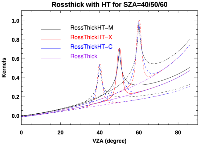
Figure 1 Four RossThick volume scattering kernels for a range of reflection zenith angles and for three solar incident angles as indicated; reflectance is in the principal plane.

Table 1 Values of N_BRDF and N_FOURIER needed to reconstruct a hotspot with ζ₀ = 1.5°.

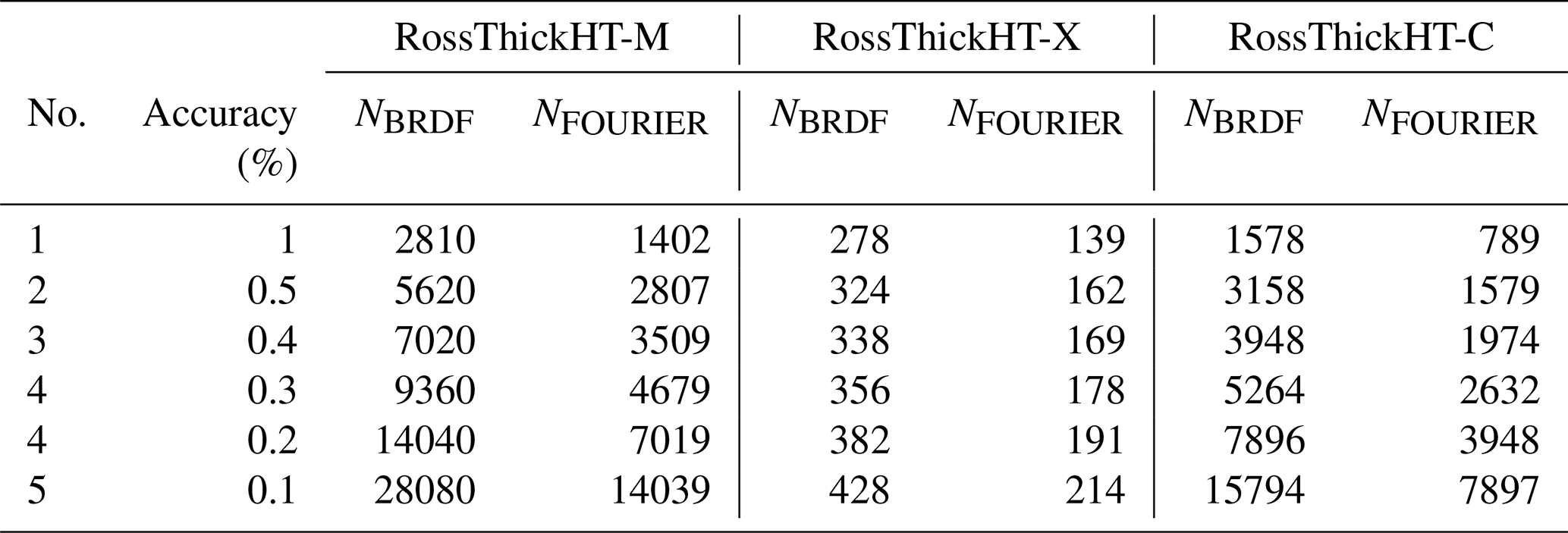
The major advantage of our new hotspot correction model is the rapid convergence for reconstruction. Table 1 lists values of N_BRDF (number of azimuth quadrature abscissae) and N_FOURIER (number of Fourier terms) that are needed to reconstruct the BRDF to different accuracy levels; the accuracy is computed as the relative difference in the reconstructed BRDF to its exact value at the hotspot. Compared to numbers required for the RossThickHT-M, values of N_BRDF and N_FOURIER for the RossThickHT-X case are 10 to 60 times smaller (Table 1). These results show that RossThickHT-X converges much faster than RossThickHT-M. We see also that convergence of RossThickHT-C is somewhat faster than that for RossThickHT-M but still much slower than that for RossThickHT-X. The computation time is roughly the third power of the number of streams. Since the number of terms used in our hotspot model is more than 10 times fewer than that specified for the original hotspot model (as shown in the Table 1), there would be a considerable performance gain with the BRDF simulations.

While both numbers are necessary for the reconstructed BRDF accuracy, the main impact comes from the number of Fourier terms N_FOURIER used when the value of N_BRDF is twice (or more) that of N_FOURIER. In Fig. 2, using a fixed value N_BRDF = 100 for the RossThickHT-M, RossThickHT-C and RossThickHT-X models, we show the dependence of the relative error in the reconstructed BRDF on the solar zenith angle for four different values of N_FOURIER. Choices of N_FOURIER (23, 31, 63 and 95) correspond to values 12, 16, 32 and 48 for the number N_STREAMS (number of half-space polar discrete ordinates) used in VLIDORT ($N_{\mathrm{FOURIER}}=\mathrm{2}{N}_{\mathrm{STREAMS}}-\mathrm{1}$). In this example, also used by Lorente et al. (2018; their Fig. 6), the BRDF represents a vegetated surface over Amazonia at wavelength 758 nm with free parameters $[P_{\mathrm{1}},P_{\mathrm{2}},P_{\mathrm{3}}]$ = $[\mathrm{0.36},\mathrm{0.24},\mathrm{0.03}]$ taken from MODIS band 2 (841–876 nm) to account for the increase in surface reflectivity near 700 nm.

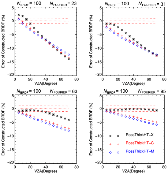
Figure 2 Accuracy of Fourier-reconstructed BRDFs relative to their exact values, for the three Ross–Li models. N_BRDF = 100, with N_FOURIER set to four different values as indicated. Surface BRDF parameters represent a vegetated surface over Amazonia at 758 nm, with $[P_{\mathrm{1}},P_{\mathrm{2}},P_{\mathrm{3}}]$ = $[\mathrm{0.36},\mathrm{0.24},\mathrm{0.03}]$.

Overall, the error decreases with increasing values of N_FOURIER. The error also increases with those viewing angles at which the hotspot occurs, since the hotspot peaks are higher and narrower for larger viewing angles. Errors for all three models are large when N_FOURIER is as small as 23. The advantage of RossThickHT-X starts to show when N_FOURIER increases to 31, but this is not significant when the hotspot viewing angle is larger than 45°. When N_FOURIER is set to 95, the performance of RossThickHT-X is much better than that for the other two models; the error is less than 1 %, even for large viewing hotspot angles, whereas the corresponding errors using RossThickHT-M or RossThickHT-C are still at the 5 %–8 % level for hotspots at viewing angles larger than 30°. Overall, the error with RossThickHT-C is slightly smaller than that for RossThickHT-M.

Next we examine the simulated TOA reflectances at 758 nm with the three hotspot models providing inputs to the main VLIDORT RT calculations. We again set N_BRDF = 100 and N_STREAMS = 12, 16, 32 and 48. Results are shown in Fig. 3 for two solar zenith angles. The hotspot signature is evident at 30° (upper panels) and 50° (lower panels), and the peak signature with aerosols present is higher than that without aerosol. The widths of the hotspots in Fig. 3 are very similar, echoing the argument of Powers and Gerstl (1988) that the hotspot width is expected to be relatively invariant to atmospheric perturbations. Lines of different colors correspond to simulations using different values of N_STREAMS; in general, differences between these lines are pretty small, especially in the atmosphere without aerosol and when the viewing angle is less than 60°. To better illustrate patterns in TOA reflectance values using different values N_STREAMS, we used the simulated reflectances obtained with N_STREAMS = 48 as the reference, and the results of this comparison are shown in Fig. 4.

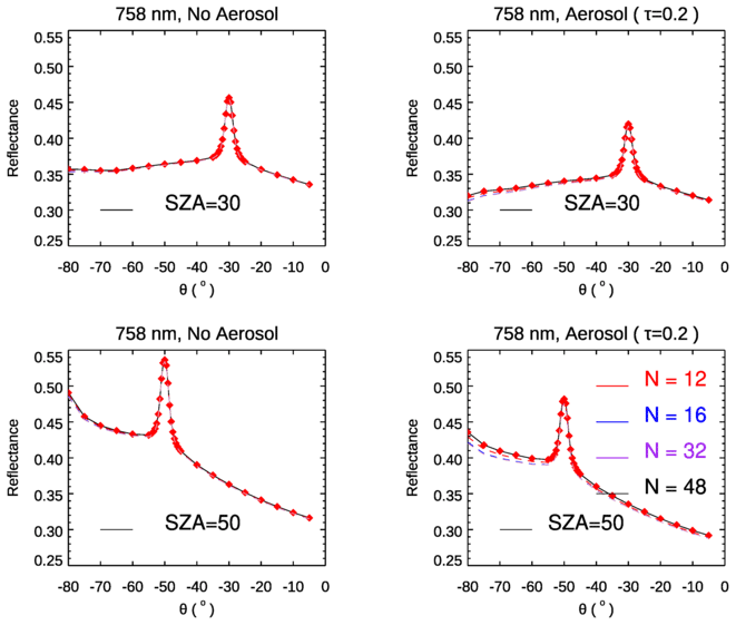
Figure 3 TOA reflectance as a function of viewing zenith angle simulated by VLIDORT at 758 nm with a Ross–Li surface BRDF model with hotspot correction RossThickHT-X. Geometries are in the principal plane for two solar zenith angles as indicated, and results were obtained with and without aerosol. Surface BRDF parameters represent a vegetated surface over Amazonia at 758 nm with $(P_{\mathrm{1}},P_{\mathrm{2}},P_{\mathrm{3}})$ = $(\mathrm{0.36},\mathrm{0.24},\mathrm{0.03})$.

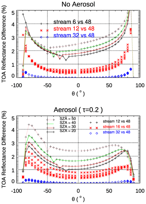
Figure 4 Same setup as Fig. 3 but now plotting the TOA reflectance differences with four solar zenith angles as indicated.

From Fig. 4 it is evident that relative differences in TOA reflectances for an atmosphere with aerosols are larger than those for the atmosphere without aerosols. As the typical viewing angle range for BRDF kernels is mostly within 60°, we will focus on these differences for viewing angles < 60°. In the upper panel, we see that TOA differences (comparing N_STREAMS = 12 with N_STREAMS = 48) increase with solar zenith angle; the difference at SZA = 50° is almost double that at SZA = 20°. The relative difference in percentage at the hotspot region is smaller than beyond the hotspot, which is easy to understand as the absolute value of the TOA reflectance at the hotspot is larger. In both cases with and without aerosol, TOA reflectance differences (comparing N_STREAMS = 32 with N_STREAMS = 48) are very small; VLIDORT simulations with N_STREAMS = 32 are accurate enough in this case.

For the atmosphere with aerosol, the bias in simulated TOA reflectances using N_STREAMS = 16 (relative to N_STREAMS = 48) is 0.5 %–1.0 %. In the clear atmosphere without aerosol, the bias of using N_STREAMS = 6 can be in the region of 2 %–3 %, but the bias with N_STREAMS = 12 is around 0.5 %, suggesting that the setting for N_STREAMS should be 12 or higher in a Rayleigh atmosphere overlying a hotspot surface.

As noted already, $N_{\mathrm{FOURIER}}=\mathrm{2}{N}_{\mathrm{STREAMS}}-\mathrm{1}$. Compared to the value of N_FOURIER needed for reconstruction of surface BRDFs near the hotspot (Table 1), that is, N_FOURIER = 139–162 for an accuracy of 0.5 %–1.0 %, the values of N_FOURIER = 23 (for the Rayleigh scenario) and N_FOURIER = 63 (for the atmosphere with aerosol) needed for full VLIDORT RT simulations are much smaller. The reason for this reduction lies with the separation in VLIDORT between the first-order (FO; single scattering and direct reflectance) calculations and the multiple-scatter (MS) calculations in VLIDORT. The first-order calculation in VLIDORT is always done with full accuracy with solar beam and line-of-sight attenuations treated for a curved atmosphere and with an exact value for the surface BRDF used to calculate the “direct-bounce” reflectance (which is very often the dominant contribution from the surface). No Fourier reconstruction is necessary for this contribution. For the MS contribution, multiple scatter is treated using Fourier cosine–sine azimuth expansions and associated Fourier terms for both the truncated-phase matrix for scattering and the diffuse-field BRDF contributions. The important point to note here is the use of the exact BRDF for the direct-bounce contribution in VLIDORT; RT models without this FO/MS separation will be constrained by the need to use a Fourier-expanded reconstruction for the direct-bounce BRDF contribution.

The results shown in Figs. 3–4 are confined to a single standard atmosphere and aerosol model. In the next section below, we use VLIDORT simulations to investigate the impact of scattering on hotspot signatures. For this study, we choose N_BRDF = 200 and N_STREAMS = 32; this should be conservative enough to avoid any uncertainty associated with the use of surface BRDFs and the choice of stream numbers in VLIDORT.

3.2 Impact of scattering on the hotspot signature at TOA

Here we use the three parameters $(P_{\mathrm{1}},P_{\mathrm{2}},P_{\mathrm{3}})=(\mathrm{0.0399},\mathrm{0.0245},\mathrm{0.0072})$ for the RTLSR surface BRDF model. These are the spatially averaged parameters from MODIS (BRDF/Albedo product MCD43A1) band 3 (459–479 nm) over Amazonia (latitude 5° N–10° S, longitude 60–70° W) for March 2008 (Lorente et al., 2018). TOA reflectances are calculated as a function of viewing zenith angle in the principal plane, with the solar zenith angle set at 30° (Fig. 5). In this experiment, we simulated two atmospheric conditions with and without aerosol and using the new hotspot correction model, RossThickHT-X, and the RTLSR BRDF model without a hotspot correction (RossThick). From the comparison of TOA reflectances at all angles between the left and the right panels in Fig. 5, we can see that the TOA reflectance in the atmosphere with aerosol is overall larger than that without aerosol, indicating that the aerosol scattering increases the TOA reflectance. Compared to the molecular scattering only, the addition of aerosol leads to an increase in TOA reflectance near the hotspot peak by ∼ 8 % and 17 % at 469 and 645 nm, respectively. However, from a comparison of the TOA reflectances with and without hotspot correction, i.e., using RossThickHT-X and RossThick, we found that at 469 nm the increase in surface reflectance at hotspot results in an increase in TOA reflectance by ∼ 4 % for atmosphere with molecular scattering only, while in the atmosphere with moderate aerosol the value of increase is only 2 %. At 645 nm, the values of reflectance increase at hotspot are about 12.5 % and 7 % for atmosphere with and without aerosol, indicating that for the longer wavelength at 645 nm, the TOA–hotspot signature is much stronger than at 469 nm. The smaller TOA–hotspot signature at 469 nm is due to the influence of stronger Rayleigh scattering. The inclusion of aerosol scattering smooths out the hotspot signature at the TOA by ∼ 44 % to −50 % compared to the atmosphere with molecular scattering only in these two wavelengths, suggesting aerosol scattering further smooths out the hotspot signature at the TOA and makes it harder to discriminate the TOA reflectance difference between the runs with and without hotspot correction. This observation agrees with the results from Bréon et al. (2002), in which it was noted that no significant hotspot signature has been observed when the surface reflectance is very small, as in the blue channel or over the ocean.

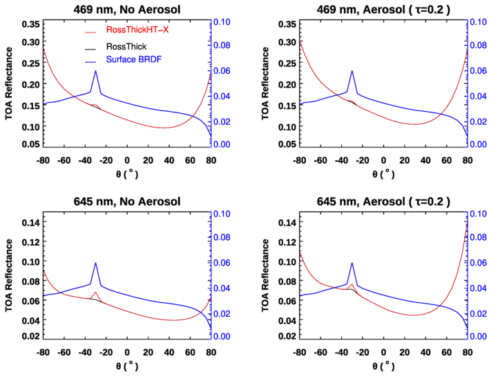
Figure 5 VLIDORT TOA reflectances as a function of viewing zenith angle with solar angle 30° in the principal plane at 469 and 645 nm, using a Ross–Li surface BRDF model RossThick and RossThickHT-X and with and without aerosol. The aerosol model used is the same as in Fig. 3, with an optical depth of 0.2. Surface BRDF parameters represent a vegetated surface over Amazonia with $(P_{\mathrm{1}},P_{\mathrm{2}},P_{\mathrm{3}})$ = $(\mathrm{0.0399},\mathrm{0.0245},\mathrm{0.0072})$, and blue curves are surface reflectance.

We also examine the hotspot signatures in 765 and 865 nm, two wavelengths used in POLDER data analysis. The three linear weighting parameters in the BRDF model are $(P_{\mathrm{1}},P_{\mathrm{2}},P_{\mathrm{3}})=(\mathrm{0.36},\mathrm{0.24},\mathrm{0.03})$, which is the same set as that used by Lorente et al. (2018). As noted already, these are taken from MODIS band 2 (841–876 nm) to account for the “red-edge” increase in surface reflectivity near 700 nm (e.g., Tilstra et al., 2017). To test the representativeness of band 2 at 758 nm, Lorente et al. (2018) scaled the parameters from band 3 (459–479 nm) using the ratio of reflectances at 772 and 469 nm; they found that differences with parameters taken from MODIS band 2 were negligible. Since we would like to focus on the difference in the impact of atmospheric scattering on the hotspot signatures at 758 and 865 nm, we have chosen to use the same two sets of surface BRDF parameters. The results are plotted in Figs. 6 and 7. To highlight the differences caused by the $\mathrm{3}\mathit{\pi }/\mathrm{4}$ factor normalizing the volume scattering kernels K_vol (see note in Sect. 2.2), we have added two simulated TOA reflectances in Fig. 7, with one based on the original hotspot correction model from Maignan et al. (2004) (RossThickHT-M) and the other using the BRDF noted in the paper of Lorente et al. (2018) (indicated by RossThickHT-L). Compared to Fig. 5, much larger TOA–hotspot signatures at both 865 and 758 nm are evident in Figs. 6 and 7, respectively, and they are slightly larger at SZA = 50° than at SZA = 30°. As expected, in the scattering region within 2° of hotspot there are some differences between RossThickHT-M and RossThickHT-X, but beyond the hotspot (±5°), the TOA reflectance using RossThickHT-X agrees very well with that using the original RossThick model. However, from Fig. 7, we see that the simulated reflectance using RossThickHT-M is slightly larger than that using RossThick model, even in a region of ±15° beyond the hotspot, particularly in the large viewing angles in the forward direction. In the region of ±5 to ±15° beyond the hotspot, the simulated reflectance using RossThickHT-M is clearly larger than that using RossThick and RossThickHT-X.

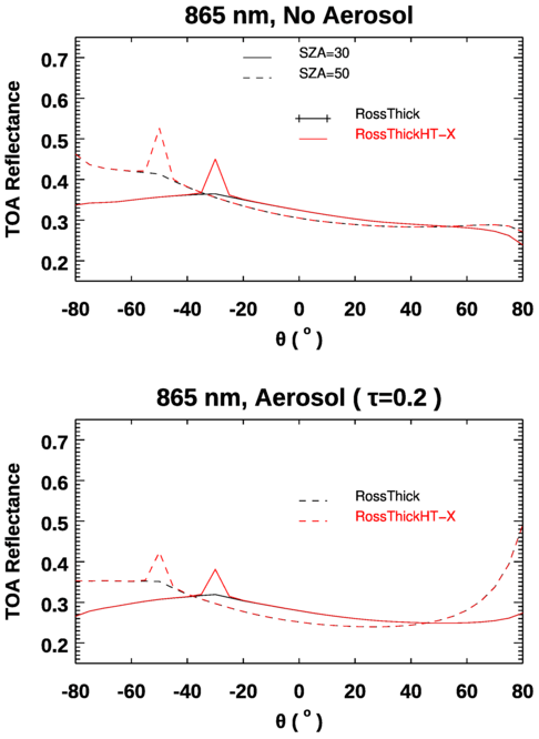
Figure 6 Same as Fig. 5 but results are calculated at 865 nm for solar zenith angles of 30 and 50°. Surface BRDF parameters represent a vegetated surface over Amazonia with $(P_{\mathrm{1}},P_{\mathrm{2}},P_{\mathrm{3}})$ = $(\mathrm{0.36},\mathrm{0.24},\mathrm{0.03})$.

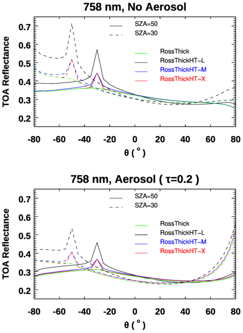
Figure 7 Similar to Fig. 6 but results calculated at wavelength 758 nm. For comparison, we have added simulated TOA reflectances using the original hotspot correction model from Maignan et al. (2004) (RossThickHT-M) and again using the model in Lorente et al. (2018), which is a factor of $\mathrm{4}\mathit{\pi }/\mathrm{3}$ times larger than RossThickHT-M in the hotspot region and is denoted here as RossThickHT-L.

To better quantify the hotspot effect and the impact due to scattering in the atmosphere, we define the “hotspot amplitude” (HS amplitude) as the difference between the TOA reflectance at the hotspot and the corresponding TOA reflectance calculated without hotspot correction, namely

$${\mathrm{HS}}_{\mathrm{Amplitude}}={\displaystyle \frac{R\left(\mathit{\theta }o,\mathit{\theta },\mathit{\varphi }=\mathrm{180},\text{RossThickHT-Li}\right)}{R\left(\mathit{\theta }o,\mathit{\theta },\mathit{\varphi }=\mathrm{180},\text{RossThick-Li}\right)}}.$$

The impacts of molecular and aerosol scattering on these amplitudes are illustrated in Fig. 8 for a range of hotspot viewing angles and for four wavelengths. For comparison, the hotspot amplitudes at the surface are also plotted. From Fig. 8, it is evident that scattering in the atmosphere smooths out the hotspot signature at TOA, and the impact of scattering is much larger in the visible compare with that in the near-infrared part of the spectrum. Even in the visible, the amplitude of the hotspot signature at 469 nm is much smaller than that at 645 nm. When the SZA increases from 20 to 50°, the HS amplitude at 469 nm decreases by −1.34 % and −1.08 % for atmospheric conditions without aerosol and with aerosol, respectively. Similarly, the HS amplitude at 645 nm decreases by −1.24 % and −2.14 %. In contrast, the HS amplitudes increase by 3.36 % (0.03 %)​​​​​​​ at 758 nm and by 3.9 % (1.5 %) at 865 nm as SZA increases from 20 to 50°. Since molecular scattering is much smaller than in the visible, the large difference in the amounts of HS amplitude increase between no-aerosol and with-aerosol conditions indicates the impact of multiple scattering, and the existence of aerosol smooths out the TOA hotspot signature. The increase in HS amplitudes with SZA following with the increase in surface reflectance in the near-infrared, particularly in the no-aerosol condition, indicates that the HS amplitude is largely affected by surface reflectance in the near-infrared.

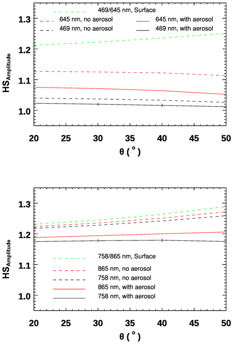
Figure 8 Comparison of hotspot amplitudes at the TOA for an atmosphere with and without aerosols in the visible (469 and 645 nm, upper) and near-infrared (758 and 865 nm, lower) ranges. Hotspot amplitudes at the surface are computed using the differences between the RossThickHT-Li and RossThick-Li BRDF models.

These simulated results agree well with the analysis of POLDER data by Bréon et al. (2002); at 440 nm, they found that the amplitude of the hotspot signature is very small. The much larger amplitudes observed at 758 and 865 nm also confirm the findings by Maignan et al. (2004), who showed that near-infrared measurements are preferred to those in the visible, not only because of the larger-amplitude directional effects but also because of the lower atmospheric perturbation. Indeed, Maignan et al. (2004) suggested that near-infrared measurement data are better suited for the evaluation of different BRDF models.

In the processing of POLDER data done by Bréon et al. (2002) and Maignan et al. (2004), only molecular scattering to first order was taken into account for the atmospheric correction. As there is no correction for the effects of aerosol scattering or the coupling of surface reflectance with molecular scattering, absolute values of the reflectances may not be fully representative of the surface for POLDER (Bréon et al., 2002). From our simulations shown in Fig. 8, the amplitude of the hotspot signature with aerosol scattering included is smaller than that without aerosol, suggesting that the results from POLDER (Bréon et al., 2002) might underestimate the amplitude of hotspot signature at the surface. Based on the differences in the HS amplitudes between the atmosphere with aerosol and without aerosol, we estimate that, on average, the HS amplitude is underestimated by 4.0 ± 1.7 % when not considering aerosol for a moderately polluted atmosphere with an optical depth of 0.2, even though most satellite observations are less affected by the aerosols than this simulation may suggest.

A final issue is related to a factor difference that exists between the equation of Lorente et al. (2018; i.e., their Eq. A1) with our Eq. (8), which is the one used in Maignan et al. (2004). The one used by Lorente et al. (2018) is $\mathrm{3}\mathit{\pi }/\mathrm{4}$ times larger; this discrepancy results in a TOA–hotspot signature that is more than twice as large, as shown in Fig. 7. Since we used the same BRDF parameters as Lorente et al. (2018), this factor difference is the main reason that the TOA–hotspot signatures shown by Lorente et al. (2018; their Fig. 5) at 469 and 645 nm from their DAK model are higher than our simulated results in this paper. In addition, in the paper of Lorente et al. (2018), the authors obtained the VLIDORT result using an older version of the code, and this result showed the hotspot peak that was smaller than that generated with the other RT models. We think the reason for this lies with a scaling factor difference between the hotspot BRDF equation cited in Lorente et al. (2018) and the equation used in the earlier VLIDORT model. Hence, we have added this simulation result here in order to bring attention to users when using scaling factor data from the MODIS BRDF product. Therefore, we caution users to be careful and check the equations for the presence of this $\mathrm{3}\mathit{\pi }/\mathrm{4}$ factor, particularly when using MODIS BRDF products.

4 Summary and conclusions

In remote sensing, it is common practice to deploy a simple kernel-driven semi-empirical model with three free parameters to represent land surface BRDFs (except snow and ice); the commonly used model is the RossThick–LiSparse combination with a correction to account for the hotspot (Maignan et al., 2004). In our study, we modified this BRDF model to improve convergence of the Fourier azimuth series decomposition. Furthermore, using this new hotspot model, we studied the impact of Rayleigh scattering and aerosol on the TOA atmospheric hotspot signature in the visible and near-infrared wavelengths using the VLIDORT RTM.

With the improved hotspot correction, we found that the numbers of Gaussian points (N_BRDF) and Fourier terms (N_FOURIER) are more than 10 times smaller than those needed with the original hotspot model from Maignan et al. (2004); this makes our BRDF model much more practical for use with VLIDORT to simulate the hotspot signature at the TOA. Another advantage of this modified model is that the new hotspot model agrees very well with the original RossThick model away from the hotspot region, thus allowing the use of this single model in the conditions with and without hotspot in applications.

We carried out a number of investigations on the impact of molecular and aerosol scattering on the hotspot signature at the TOA. TOA reflectances were calculated for different solar and viewing angles and at four wavelengths. These simulations using VLIDORT show the following:

1. In agreement with previous analysis using POLDER measurement data, hotspot signatures in the near-infrared are larger than those in the visible, as it is less impacted by scattering molecules, making it better for deriving the surface hotspot signature.

2. In agreement with the POLDER study, the hotspot amplitudes at TOA and the surface both increase with solar zenith angle in the near-infrared; however, at 469 and 645 nm, this increase with solar zenith angle is not obvious at TOA, due to stronger Rayleigh scattering at shorter wavelengths, which is more pronounced for longer path lengths at larger solar zenith angles.

3. Scattering by molecules and aerosols in the atmosphere tends to smooth out the hotspot signature at TOA, and the hotspot amplitude is reduced when aerosols are added to an otherwise clear (Rayleigh-scattering-only) atmosphere.

4. In VLIDORT, the direct-beam solar reflectance is calculated using the exact BRDF (rather than in a truncated Fourier series form); this means that smaller values of N_FOURIER (i.e., 23 and 63 for atmospheres without and with aerosol scattering) can be used in for the multiple-scattering calculations in VLIDORT to obtain hotspot signature with acceptable accuracy.

Since atmospheric corrections in the POLDER data processing were performed using Rayleigh-only single scattering without any consideration of aerosol, we found from our simulations that the amplitude of hotspot signature at the surface is likely underestimated by 4.0 ± 1.7 % in the analysis of hotspot signature using POLDER data (Bréon et al., 2002), highlighting the importance of considering the multiple scattering and including aerosols in the retrievals of surface BRDF (hotspot).

Our improved hotspot kernel is now a standard feature in the latest version of the VLIDORT BRDF supplement code that significantly improves the numerical efficiency. Since this new model has not been validated using any real observation data, and considering the difference between this model and the original hotspot model from Maignan et al. (2004) in scattering angles close to the peak of hotspot, it may not be appropriate for those who need an exact representation of the hotspot angular signature around the peak of hotspot.