A multi-decadal time series of upper stratospheric temperature profiles from Odin-OSIRIS limb-scattered spectra

A new upper stratospheric (35–60 km) temperature data product has been produced using Optical Spectrograph and InfraRed Imager System (OSIRIS) limb-scattered spectra that now spans over 22 years. Temperature is calculated by first estimating the Rayleigh scattering signal and then integrating hydrostatic balance combined with the ideal gas law. Uncertainties are estimated to be 1–5 K, with a vertical resolution of 3–4 km. Correlative comparisons with the Atmospheric Chemistry Experiment Fourier Transform Spectrometer (ACE-FTS) and the Microwave Limb Sounder on Aura (MLS) are consistent with these uncertainty estimates and generally have no regions of statistically significant drift. The data product has been publicly released as part of the nominal OSIRIS v7.3 processing.

1 Introduction

Stratospheric cooling over the past several decades is a key sign of anthropogenic climate change (e.g., Gulev et al., 2021). In order to monitor temperature variations on climate time scales it is necessary to have an observational dataset that extends for multiple decades. It has thus far been difficult to quantify the magnitude of stratospheric cooling due to a deficit of long-term and vertically resolved observational datasets, particularly in the upper stratosphere where observations from Global Navigation System (GNSS) Radio Occultation (RO) measurements are highly uncertain (Steiner et al., 2020a). Temperature trend studies in the middle and upper stratosphere have largely relied on merged datasets with limited vertical resolution (e.g., Randel et al., 2016; Steiner et al., 2020b; Maycock et al., 2018; Randel et al., 2017). Global trends from these studies for the ozone recovery period (post ∼ 1998) range from −0.19 K per decade (Randel et al., 2016) to −0.5 K per decade (Steiner et al., 2020b) near 40 km, and from −0.28 K per decade (Randel et al., 2016) to −0.6 K per decade (Steiner et al., 2020b) near 45 km. This relatively large uncertainty in upper stratospheric cooling limits our ability to understand the response of the stratosphere to anthropogenic climate change and spurs the development of a new stratospheric temperature product.

Several studies have demonstrated the ability to retrieve stratospheric and mesospheric temperature profiles from limb scatter measurements. The first demonstration was via the visible light spectrometer on board the Solar Mesosphere Explorer satellite (Rusch et al., 1983). Sheese et al. (2012) used spectra from the Optical Spectrograph and Imager System (OSIRIS, Llewellyn et al., 2004) to determine temperatures in the range 55–80 km and Hauchecorne et al. (2019) used Global Ozone Monitoring by Occultation of Stars (GOMOS, Kyrölä et al., 2004) daytime limb observations to retrieve temperature in the 35–85 km range. While these methods differ in algorithmic details, they share a common core procedure of using isolated wavelengths in the UV–Vis to retrieve Rayleigh scattering number density and then using a combination of hydrostatic balance and the ideal gas law to estimate temperatures, which goes back to a technique developed for LIDAR sensors by Hauchecorne and Chanin (1980). In limb scatter measurements there is an additional complication of multiple scattering in the atmosphere and the prior methods for OSIRIS and GOMOS both assume that multiple scattering in the atmosphere can be neglected. Chen et al. (2023) retrieved temperatures from 35–75 km with Ozone Mapping and Profiler Suite Limb Profiler (OMPS-LP, Flynn et al., 2004) measurements using a similar technique; however, a multiple scattering correction along with altitude normalization was performed to improve the retrieval at lower altitudes.

Recently, the primary OSIRIS data products (ozone, nitrogen dioxide, and stratospheric aerosol) have been updated to v7 and described in several publications (Bognar et al., 2022; Rieger et al., 2019; Dubé et al., 2022). One key improvement in the processing chain is that all of these products are processed self-consistently rather than separately as was done in the past. Included in this new v7 processing chain is the retrieval of stratospheric temperature. The profiles are derived through a multi-stage procedure of estimating the Rayleigh scattering signal from OSIRIS spectra and then integrating hydrostatic balance combined with the ideal gas law. The useful range of these profiles is approximately 35–60 km. The temperature data product is publicly distributed as part of the recently released OSIRIS v7.3 data products. An example of the produced data is shown in Fig. 1. The technique differs from previous techniques in that multiple scattering is included rigorously in the forward model, with a novel method to estimate the amount of upwelling radiation.

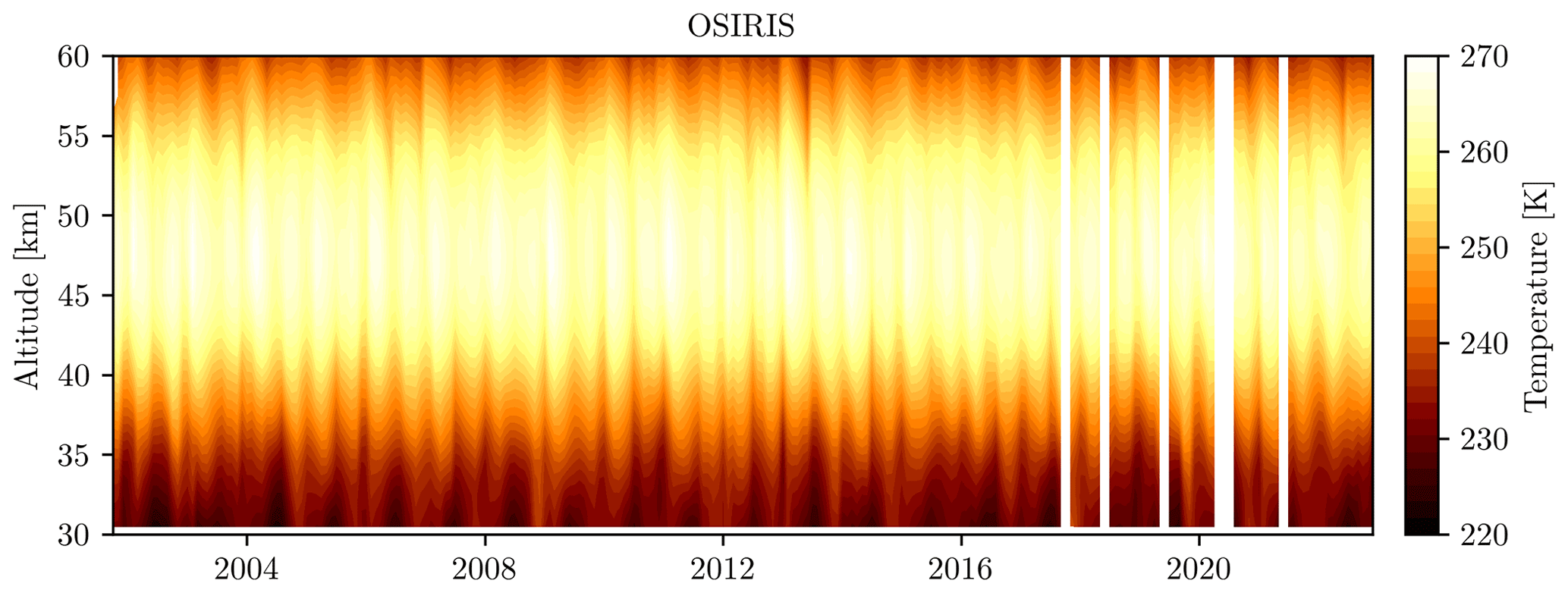
Figure 1 Tropical (20° S to 20° N) monthly zonal mean time series calculated from the OSIRIS v7.3 temperature data product.

Section 2 describes the OSIRIS measurement technique, while the retrieval technique is given in Sect. 3. The associated sensitivity studies and internal assessments are presented in Sect. 4 and intercomparisons with other instruments are given in Sect. 5. A future publication is being prepared which relates the full OSIRIS temperature time series to reanalysis datasets.

2 OSIRIS limb scatter measurements

The Swedish satellite Odin (Murtagh et al., 2002) was launched in 2001 and continues to make atmospheric measurements resulting in an ongoing time series of more than 22 years. One of two instruments on board, OSIRIS, measures limb-scattered sunlight in the 280–800 nm spectral region, using a diffraction grating to disperse the signal with a spectral sampling and resolution of about 1 nm. Odin continuously scans the atmosphere in the vertical direction to obtain altitude-resolved spectra. Each scan takes approximately 90 s, with a tangent altitude spacing of 2–3 km. Odin primarily operates in three scanning modes: Strat, Meso, and Strat+Meso. The majority of Odin scans (especially in recent years) are in the Strat mode, which scans the stratosphere from the surface to ∼ 65 km.

Odin is in sun-synchronous orbit with a local time at ascending node of ∼ 18:00, which causes the majority of measurements to be made at times near dawn or dusk. Since Odin's orbit is not controlled, the local time has drifted later over time, in many cases causing the ascending node to drift past the 88° solar zenith angle cutoff used by the retrieval. Since this drift does not affect the sampling of the AM, or the descending node measurements, in this study we focus only on the AM measurements. On average, this results in ∼ 100 measurements per day across the entire mission.

3 Method

Stratospheric temperature is retrieved from OSIRIS limb scatter measurements in a two-step procedure. First, Rayleigh scattering number density is inferred from radiances at 310 and 350 nm. Next, the number density is used in conjunction with hydrostatic balance and the ideal gas law to obtain temperature. Here we describe the method used to obtain stratospheric temperature from OSIRIS limb-scattered radiances. The temperature retrieval steps are described in reverse order, beginning with the process of determining temperature from the Rayleigh scattering number density as we believe this is most informative.

3.1 Temperature determination

Knowing the Rayleigh scattering number density as a function of altitude, n(z), it is possible to determine atmospheric temperature. The conversion follows almost identically to that of Sheese et al. (2012), Hauchecorne and Chanin (1980), and Hauchecorne et al. (2019), where hydrostatic balance and the ideal gas law are combined to obtain

$$\begin{array}{}\text{(1)}& T\left(z\right)={\displaystyle \frac{\mathrm{1}}{n\left(z\right)}}\left(n\right(z_{\mathrm{0}}\left)T\right(z_{\mathrm{0}})-{\displaystyle \frac{\mathrm{1}}{k}}\underset{z_{\mathrm{0}}}{\overset{z}{\int }}g(z^{\prime }\left)n\right(z^{\prime }\left)m\right(z^{\prime }\left)\mathrm{d}{z}^{\prime }\right),\end{array}$$

where T(z) is the temperature profile at altitude z, g is local gravitational acceleration, k is the Boltzmann constant, m is the mean molecular mass of air, and z₀ is a reference altitude. The application of Eq. (1) is straightforward with numerical integration techniques as long as temperature at a reference altitude is known. Sheese et al. (2012) opted to pin the reference altitude at ∼ 85 km, and to calculate the reference temperature from an estimate using OSIRIS A-band emission spectra (Sheese et al., 2010); however, this is only possible for Odin-OSIRIS scans in stratospheric–mesospheric mode. Instead, we calculate the temperature profile using two different reference values at the upper limit of the retrieved Rayleigh scattering number density.

The first reference value is an interpolated MERRA2 (Gelaro et al., 2017) profile used in the standard OSIRIS processing. This value is a reasonable estimate of the mesospheric temperature (Long et al., 2017) and it most likely produces the most accurate OSIRIS temperature profile; however, any spurious trend in the MERRA2 data at the reference altitude will be aliased into the OSIRIS temperature values. To obtain more robust trend estimates, we compute a second temperature profile pinned by a climatological value estimated from the NRLMSISE-00 model (Picone et al., 2002). Differences in these two temperature products are assessed in the following sections.

There are two natural ideas to take note of with Eq. (1). First, the temperature profile does not depend on the magnitude of the retrieved Rayleigh scattering number density, only on its shape. In other words, scaling the retrieved number density profile by a constant factor does not change the retrieved temperature profile. The scaling invariance provides some robustness to errors either in the instrument calibration or in radiative transfer modeling. The second is that errors in the reference temperature directly introduce errors in the retrieved profile; however, these errors drop off exponentially in altitude and can be immediately estimated.

3.2 Rayleigh scattering number density retrieval

Rayleigh scattering number density is retrieved using a standard optimal estimation retrieval scheme (Rodgers, 2000). The state vector, x, consists of the logarithm of dry air number density on an altitude grid and is updated iteratively through the relation

$$\begin{array}{}\text{(2)}& {\mathit{x}}_{i+\mathrm{1}}={\mathit{x}}_i+\left[{\mathbf{K}}^T{\mathbf{S}}_y^{-\mathrm{1}}\mathbf{K}+{\mathbf{\Gamma }}^T\mathbf{\Gamma }\right]{\mathbf{K}}^T{\mathbf{S}}_y(\mathit{y}-F({\mathit{x}}_i\left)\right),\end{array}$$

where y is OSIRIS-measured radiance at 350 nm, S_y is the error covariance matrix of these measurements, Γ is a second-order Tikhonov regularization matrix, K is the Jacobian matrix, and F is a combination of an OSIRIS instrument model and the SASKTRAN radiative transfer model (Zawada et al., 2015). Included in the forward model calculation are the OSIRIS v7 estimates of stratospheric aerosol, ozone, and nitrogen dioxide. The Jacobian matrix is calculated analytically by the SASKTRAN radiative transfer model (Zawada et al., 2017). The logarithm of dry air number density is used since its second derivative is approximately 0 inside the Earth's atmosphere.

The state vector is represented on a 1 km uniform altitude grid beginning at 30 km and extending to the top of the OSIRIS scan or to 80 km, whichever is lower. We expect that any measurement below ∼ 35 km is contaminated by the effects of stratospheric sulfate aerosol; setting the lower bound at 30 km allows us to test this assumption without adversely affecting the entire profile. Most of the time, OSIRIS operates in stratospheric mode where each scan stops at ∼ 65 km; in these cases the scan top is set as the upper limit of the state vector. OSIRIS can also operate in a mesospheric mode, where the scan extends to ∼ 100 km or above. Here the upper limit is set to 80 km to avoid regions of significant stray light. Above the upper bound and below the lower bound the number density profile is scaled by a constant factor to line up with the state vector at each iteration.

The second-order Tikhonov factor is chosen in a semi ad hoc fashion so that the average χ² value, calculated through

$$\begin{array}{}\text{(3)}& {\mathit{\chi }}^{\mathrm{2}}={\displaystyle \frac{{\left(\mathit{y}-F\left(\widehat{\mathit{x}}\right)\right)}^T{\mathbf{S}}_y\left(\mathit{y}-F\left(\widehat{\mathit{x}}\right)\right)}{M-\mathrm{1}}},\end{array}$$

where M is the number of measurements, is approximately equal to 1. This criterion minimizes the amount of overfitting done by the retrieval and results in a mean vertical resolution of 3–3.5 km (see Sect. 4.3.5).

3.3 Lambertian-equivalent reflectance estimation

Radiances at 350 nm contain significant signal from multiple scattering. Multiple scattering in this wavelength region is primarily an upwelling radiation effect: light scatters either at the ground or the cloud top and undergoes multiple scattering events until scattering a final time along the instrumental line of sight. Accounting for every physical process in this scattering path is not feasible both from a lack of atmospheric composition information and also from the large increase in radiative transfer modeling complexity. Instead, we assume a clear sky troposphere and a Lambertian reflectance at the Earth's surface parameterized by a scalar, spectrally invariant, surface albedo. Prior to beginning the Rayleigh scattering number density retrieval, we estimate the surface albedo.

For the OSIRIS v7 retrievals of ozone, stratospheric aerosol, and nitrogen dioxide, surface albedo is required and retrieved; however, this estimate is not suitable for use in the temperature retrieval. The primary surface albedo estimated is retrieved at 675 nm to be applicable for wavelengths in the aerosol retrieval and Chappuis ozone absorption bands; however, the albedo at this wavelength may be significantly different than that at 350 nm. The method used also cannot simply be repeated at 350 nm. Absolute radiances at a high altitude can be used to estimate the surface albedo; however, these radiances at 350 nm are already used in the retrieval of Rayleigh scattering number density and do not contain any independent pieces of information for surface albedo. Instead, a new method has been developed to estimate surface albedo in this region.

Our goal is to obtain a piece of information in the OSIRIS radiances that varies with surface albedo but is approximately independent of Rayleigh scattering number density and ozone absorption, which are the primary radiative effects in this wavelength region. Simulations were performed in the nearby spectral area using varying amounts of ozone and surface albedo at an altitude of 60 km and are shown in Fig. 2. At 350 nm, the spectrum is only sensitive to the underlying surface albedo. From 310 to 340 nm, we see dependence on the atmospheric ozone profile. However, this dependence is not through absorption along the line of sight but through attenuation of the multiply scattered upwelling signal. Direct line-of-sight sensitivity to ozone begins around ∼ 295 nm and continues to increase as the wavelength decreases. The spectral range of ∼ 295 to ∼ 305 nm is generally insensitive to both the atmospheric ozone profile and the surface albedo.

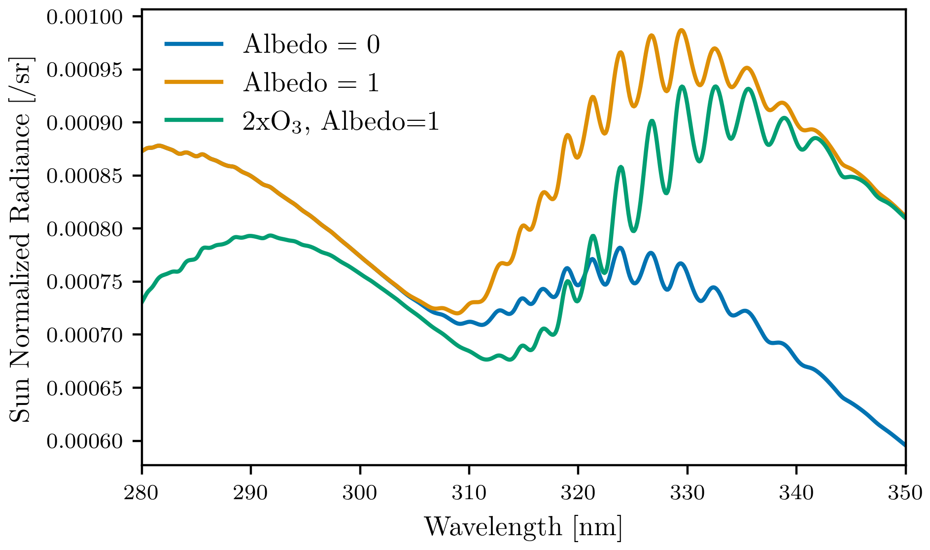
Figure 2 Sun-normalized radiance spectra as simulated by SASKTRAN at 60 km for three different scenarios. “Albedo 0”: standard atmosphere, surface albedo set to 0. “2× O₃”: atmosphere with twice as much ozone, albedo set to 1. “Albedo 1”: standard atmosphere, surface albedo set to 1.

To retrieve effective surface albedo we define the measurement vector,

$$\begin{array}{}\text{(4)}& y_a=\log I(\mathrm{350}\mathrm{nm},\mathrm{60}\mathrm{km})-\log I(\mathrm{305}\mathrm{nm},\mathrm{60}\mathrm{km}),\end{array}$$

which is approximately insensitive to both Rayleigh scattering number density and ozone absorption, but retains sensitivity to the surface albedo. The retrieval then proceeds by setting the state vector to be the scalar surface albedo and performing an unregularized form (Γ=0) of Eq. (2). Since SASKTRAN is unable to analytically compute the derivative of surface albedo, we calculate the measurement vector once with an albedo of 0 and estimate the derivative as

$$\begin{array}{}\text{(5)}& {\displaystyle \frac{\partial I}{\partial a}}=K={\displaystyle \frac{y_a\left(a\right)-y_a\left(\mathrm{0}\right)}{a}}.\end{array}$$

Using an approximate Jacobian most likely increases the number of iterations required in the retrieval, but reduces computation time overall since the problem is sufficiently linear.

We have noticed that many scenes result in the retrieval wanting to push the albedo to negative. Rather than allowing a negative albedo in SASKTRAN, we leave the albedo at the minimum value and add a flat absorber to the troposphere. The absorber is assumed to have a constant number density from 0–5 km and have a spectrally flat cross section. The state vector element is then switched from albedo to vertical optical depth of this absorber. The Jacobian is estimated in a fashion similar to Eq. (5) using the previously computed radiance at an albedo of zero. Currently any scene where an absorber is added is recommended to be filtered out, this happens in approximately 7.1 % of measured scans.

4 Internal assessment and sensitivity studies

4.1 Absolute calibration effect

As previously noted, a scaling of the retrieved Rayleigh scattering number density does not directly influence the retrieved temperature profile. However, only in certain conditions does a multiplicative scaling of the radiance profile (e.g., absolute calibration error) directly result in a scaling of the retrieved number density profile. The two sufficient conditions are (a) that the fraction of multiple scatter is constant as a function of altitude and (b) that the optical depth along the limb line of sight is sufficiently small that attenuation from the Beer–Lambert law is linear. Generally these two conditions are met at higher altitudes in the atmosphere and start to become significant at altitudes below 40–45 km. Section 4.1 quantifies this effect through simulation.

Little effort has been put into characterizing the absolute calibration of OSIRIS during the multi-decade mission. Most of the other retrieved OSIRIS data products (ozone, stratospheric aerosol, nitrogen dioxide) are only weakly sensitive to the absolute calibration through coupling with the estimated surface albedo. The platform itself also contains no on-board calibration sources and is unable to directly measure known brightness features that fully illuminate the slit. An updated OSIRIS absolute calibration has been developed specifically to improve the temperature retrieval data product.

OSIRIS-measured radiances are compared with SASKTRAN simulations using reanalysis atmospheric inputs over time for specific measurement geometries that we are confident can be simulated accurately. We restrict ourselves to scans with a tangent point solar zenith angle of ∼ 90°, which minimizes the amount of upwelling radiation, and solar scattering angles of ∼ 90°, which limits the change in solar zenith angle along the line of sight. Larger solar zenith angles may further increase the relative importance of single scattering; however, solar zenith angles above 90° result in the solar beam passing through altitudes below the measurement tangent point, which is undesired. Only high-altitude measurements (tangent altitudes near ∼ 60 km) are used to minimize the impacts of unknown ozone concentrations for the UV wavelengths. The exact latitudes, longitudes, and seasonality of these measurements vary from year to year due to drifts in the Odin orbit.

The results of the absolute calibration procedure are shown in Fig. 3. Only annual mean data are used to attempt to minimize variations in sampling. A logistic curve is fit to the annual mean data to create a smoothly varying correction that varies only in time and wavelength. Curiously, over time the signals observed from OSIRIS have increased and not decreased. The mechanism for the increase is unknown, but it may be related to a coating that was applied to the UV portion of the detector. Much of the variation within each year may be caused by uncertainties in the OSIRIS absolute pointing (Bourassa et al., 2018); however, since the determination of the absolute pointing is relatively insensitive to the absolute calibration, we do not expect there to be significant biases due to pointing uncertainty.

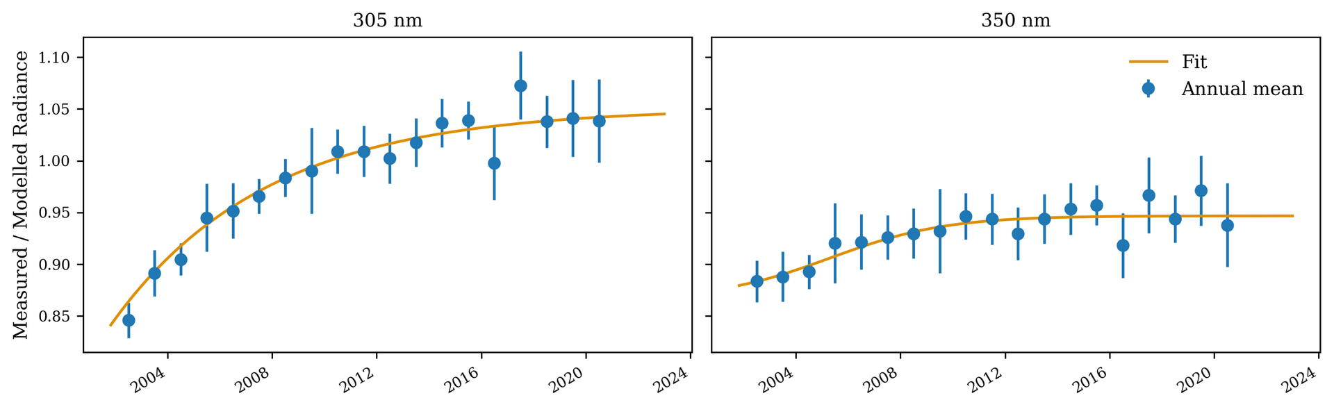
Figure 3 Annual mean measured radiances divided by modeled radiances at 60  km for the absolute calibration scenarios described in the text (blue dots) and their associated 1σ uncertainties (error bars) at the two wavelengths used in the temperature product retrieval. The orange curve shows the result of fitting a logistic curve to the data and is the curve that is applied to OSIRIS data.

As an initial assessment of the new absolute calibration, we compared the v7.3 temperature data product with a special processing version, with the only difference being that it did not contain the absolute calibration correction in Fig. 4. We analyze the lowest usable altitude (35.5 km), since low altitudes are both affected by errors in absolute calibration (see Sect. 4.1) and are expected to be more accurate in MERRA2. Without the absolute calibration, a significant (−2.43 ± 0.43 K per decade) drift is observed relative to MERRA2. With the new absolute calibration the drift becomes insignificant (−0.22 ± 0.23 K per decade). Potential drifts at low altitudes are further examined in Sect. 5.4.

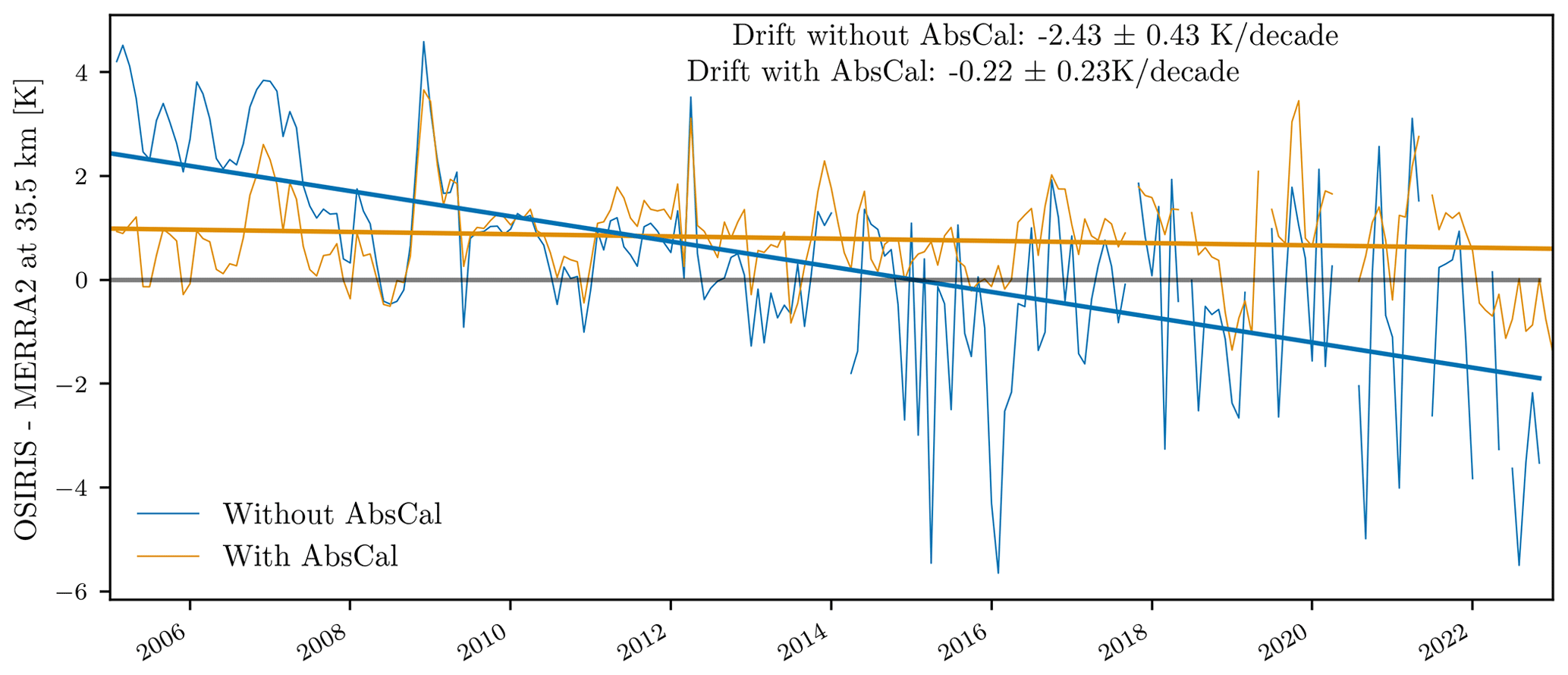
Figure 4 Monthly zonal mean differences between OSIRIS and MERRA2 at 35.5 km in the 10° S to 10° N latitude band with and without the new absolute calibration. Linear fits to each time series are shown with associated 2σ error estimates.

4.2 Aerosol contamination at low altitudes

The limiting factor in pushing the retrieval lower into the stratosphere is the presence of stratospheric aerosol scattering. It is difficult to decouple the scattering effect of aerosols from that of Rayleigh scattering particles. The temperature retrieval includes the OSIRIS v7 retrieved aerosol extinction as an ancillary parameter; however, this retrieval primarily uses information from longer wavelengths (Rieger et al., 2019). Uncertainties in the aerosol particle size distribution and composition can introduce significant errors in the shorter wavelengths that are used in the temperature retrieval. Rather than setting the retrieval lower bound at a safe altitude where we are certain there is no aerosol influence (e.g., 40 km), we have opted to set the lower bound to an altitude that we know will be contaminated with aerosol (30 km) and then to post-filter the data.

Since the OSIRIS v7 aerosol profile is used as ancillary data inside the retrieval, it is not the presence of aerosol itself that causes errors in the retrieval, but rather the uncertainties due to unknown aerosol particle size and composition. Therefore, we determine which altitudes are adversely affected by aerosol uncertainties by analyzing correlations with the single scattering angle (SSA). Similar ideas have been used to analyze errors of unknown aerosol particle size in retrieved aerosol extinction. Figure 5 shows the tropical monthly zonal mean differences relative to the MERRA2 ancillary data as a function of SSA for different altitude levels. At the lowest retrieved altitude (30.5 km), we see a strong dependence on SSA, with temperature differences varying almost linearly from 5 to −5 K over the 50° of observed OSIRIS scattering angles. The dependence decreases with increasing altitude, as expected with decreasing aerosol concentrations. At 35.5 km the observed scattering angle dependence decreases to ±0.5 K and stays below that level for all altitude levels above it. Therefore, we recommend that the retrieved temperature data product not be used at altitude levels below 35 km.

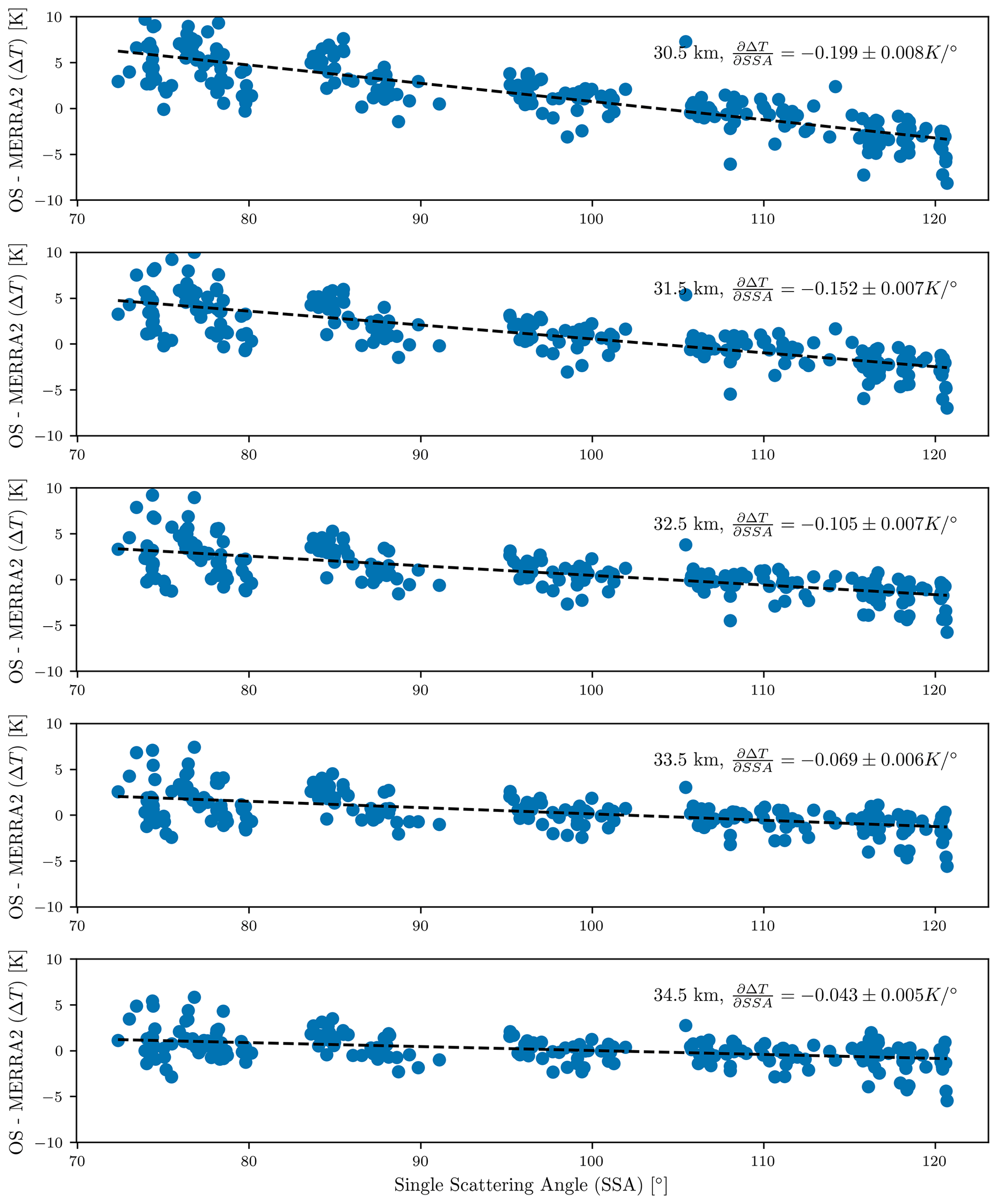
Figure 5 Differences between OSIRIS and MERRA2 at a set of tangent altitudes as a function of single scattering angle in the 10° S to 10° N latitude band for the entire mission time period. Slopes are shown with associated 2σ error estimates.

4.3 Error analysis

We have identified three primary sources of error that influence the retrieved temperature data product: (1) error due to errors in the assumed reference temperature; (2) error due to random noise present within the OSIRIS spectral measurements; and (3) error from errors in the absolute signal level of the measurements, primarily originating from errors in the instrumental absolute calibration. To assess these errors we processed 100 OSIRIS orbits from the year 2009 chosen randomly with different retrieval configurations. The following subsections outline the setup of these tests and highlight the results.

4.3.1 Reference temperature errors

Errors due to errors in the reference temperature are estimated by comparing the retrieved temperature that uses NRLMSISE-00 as the reference temperature to the retrieved temperatures pinned to the MERRA2 value. Differences between these two values provides a conservative estimate for uncertainty at the reference temperature. The mean differences observed for the 100 test orbits is shown in Fig. 6. Near the reference altitude, both the mean difference and observed scatter approach 5 K, decreasing exponentially with decreasing altitude.

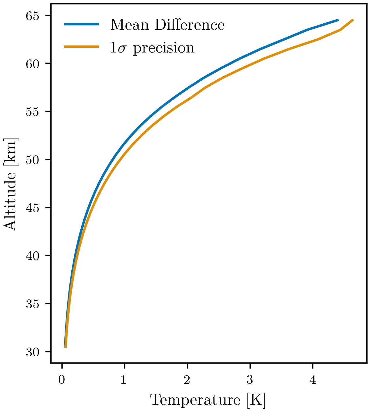
Figure 6 Mean differences and 1σ standard deviation between the NRLMSISE-00 pinned and MERRA2 pinned temperature data products for the 100 test orbits.

The exponential decrease in error with decreasing altitude can be directly seen from Eq. (1). An error in the pinning temperature, δT(z₀), directly results in an error in the retrieved temperature profile:

$$\begin{array}{}\text{(6)}& \mathit{\delta }T\left(z\right)={\displaystyle \frac{n\left(z_{\mathrm{0}}\right)\mathit{\delta }T\left(z_{\mathrm{0}}\right)}{n\left(z\right)}}.\end{array}$$

At the nominal reference altitude, 65 km, we observe mean differences of 5.6 K between the climatological NRLMSISE-00 value and the interpolated MERRA2 temperatures, with a standard deviation of 5.1 K. The error in the retrieved profile can be estimated directly from the retrieved number density, but owing to the exponential nature of the atmospheric density profile it is well approximated through the relation

$$\begin{array}{}\text{(7)}& \mathit{\delta }T\left(z\right)=\exp \left(-{\displaystyle \frac{z_{\mathrm{0}}-z}{z_{\mathrm{s}}}}\right)\mathit{\delta }T\left(z_{\mathrm{0}}\right),\end{array}$$

where z_s is the scale height of the atmosphere (∼ 8.5 km). From this relation we can see that the temperature error due to errors in the reference temperature decreases exponentially in altitude and for a reference altitude of 65 km, the error reaches a 10-fold reduction at approximately 45 km.

4.3.2 Random noise

We assess the random-noise component in two, somewhat equivalent, ways. The random-noise component of the retrieval can be estimated through standard linear error analysis. For details on how this is applied to the derived temperature product, see Appendix B. The OSIRIS signal-to-noise ratio (SNR) is approximately ∼ 500 for the wavelength used in the retrieval and has minimal variation in altitude or viewing condition since an auto-exposure time process is used during nominal operation. Since almost the entire signal originates from Rayleigh scattering, the precision in the retrieved number density, and in the temperature values, is expected to be very close to this SNR value.

The second method to determine the random component of the retrieval is to change the wavelength used to retrieved Rayleigh scattering number density. For this test, we move the retrieval wavelength to 345 from 350 nm, with the results shown in Fig. 7. The observed scatter matches closely with the predicted scatter and is a constant 0.8 K from 35 to 55 km, increasing slightly to values marginally greater than 1 K at higher altitudes. We believe the slight deviation between the two methods at 60 km is caused by pseudo-systematic errors in the radiance at the upper retrieval limit, most likely stray light. A small −0.2 K mean bias is observed when moving the wavelength to 345 nm. The cause of the bias is unknown, but it does suggest that there is the potential for small, most likely constant in time, biases in the retrieved temperature depending on the exact OSIRIS wavelength chosen. The current wavelength of 350 nm was chosen because this pixel is used in the operational OSIRIS ozone retrieval and is well understood. A future version of the data product will explore improving the precision by using multiple wavelengths.

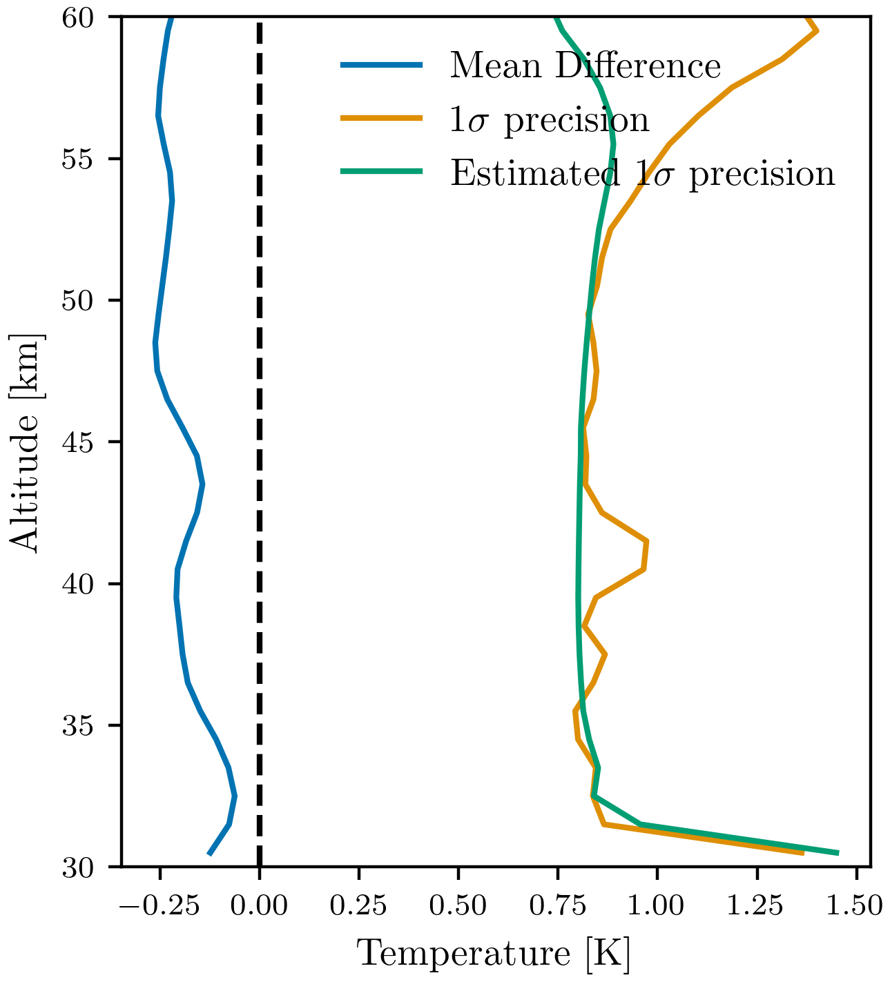
Figure 7 Mean differences and 1σ standard deviation for the 100 test orbits when the nominal retrieval wavelength is moved to 345 from 350 nm.

4.3.3 Absolute calibration error

The temperature retrieval uses two distinct wavelengths, 350 and 305 nm. Errors in the absolute calibration of each of these channels will alias into errors in the retrieved temperature values. The primary mechanism for the introduced error is non-linearity of the radiative transfer equation as we move lower into the atmosphere. Based on the technique to determine the absolute calibration described in Sect. 4.1, we expect errors in the estimated absolute calibration to be highly correlated between these two measurements. Therefore to assess errors in the absolute calibration, we artificially multiply the observed radiance by a spectrally flat value of 1.05. The results of the test are shown in Fig. 8.

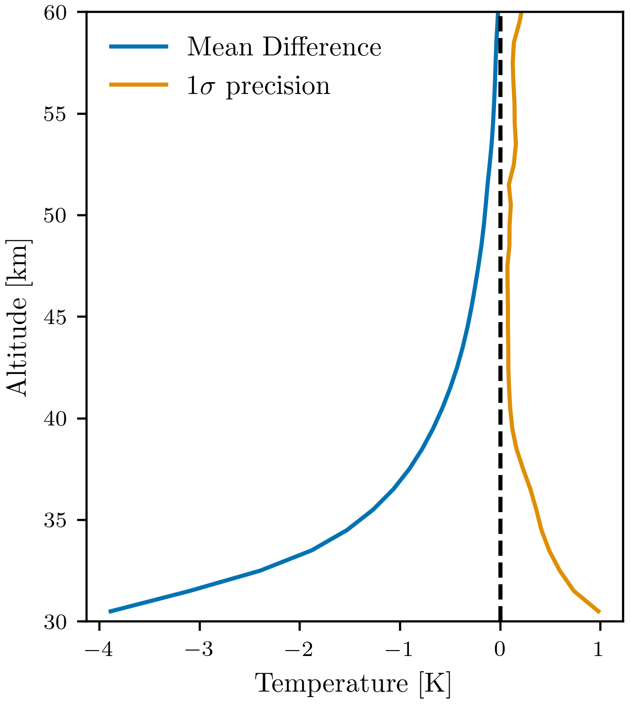
Figure 8 Mean differences and 1σ standard deviation for the 100 test orbits when the OSIRIS absolute radiances are artificially scaled by 1.05.

There is a small increased scatter from the absolute calibration scaling; however, above 35 km it is less than 0.3 K and likely is a result of the non-linear nature of the problem. The bias introduced from the absolute calibration scaling appears to increase exponentially with decreasing altitude, reaching −1 K at 37.5 km. At the lowest usable altitude of the retrieval, 35 km, the mean retrieved temperature difference nears −2 K for a 5 % change in absolute radiance.

4.3.4 Other potential forms of bias

While the previous three sections outline what we believe to be the primary sources of error in the retrieved temperature data product, there do exist other sources of error for the retrieved data product. In addition, we have tested the retrieval sensitivity to:

• the assumed aerosol particle size in the aerosol retrieval by increasing the log-normal median radius from 80 to 100 nm,

• the neglect of polarization in the retrieval forward model by including the effects of polarization in the calculation,

• the wavelength used in the equivalent Lambertian reflectance retrieval by switching the wavelength from 305 to 307 nm,

• a pointing knowledge shift of 100 m at the tangent point (implemented as a constant angular shift in the OSIRIS pointing frame with a mean tangent altitude shift of 100 m).

The results of these studies are shown in Fig. 9.

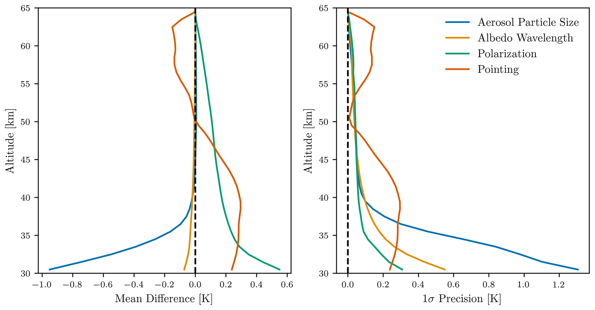
Figure 9 Mean differences and 1σ standard deviation for the 100 test orbits for perturbations in aerosol particle size, albedo retrieval wavelength, and simulating polarization in the retrieval forward model. See text for details.

Generally, all four effects introduce very little bias in the retrieved temperature data product. Aerosol particle size and the wavelength used for the albedo retrieval are negligible above 35 km. The neglect of polarization and potential pointing errors have the largest bias, introducing a bias on the order of 0.2 K above 35 km. We note that polarization errors are partly canceled from the absolute calibration correction. A 100 m pointing shift causes biases of ±0.25 K depending on the direction of the shift and whether or not the altitude is above or below the stratopause. The scatter of the aerosol particle size, albedo wavelength, and polarization effects is less than 0.1 K above 40 km and rapidly increases below that. The aerosol particle size effect is the largest, increasing to 0.6 K at 35 km. Owing to the large uncertainties in stratospheric aerosol composition, it is not unreasonable to expect that errors larger than this could be observed in the 35–40 km altitude region in time periods of enhanced aerosol.

4.3.5 Vertical resolution

The vertical resolution of the Rayleigh scattering number density retrieval is available through the retrieval averaging kernel; however, the averaging kernel for the temperature data product is not the same due to the conversion in Eq. (1). Note that since the temperature conversion is non-linear, there is no exact conversion from the Rayleigh scattering number density averaging kernel to the temperature averaging kernel. The proper way to apply the averaging kernel to a comparison dataset would be to convert to number density, apply the averaging kernel, then re-apply Eq. (1). However, since the temperature at a specific level is primarily influenced by the number density at that level (see Eq. A9), the vertical resolution of the number density retrieval provides a rough estimate of the vertical resolution of the temperature data product.

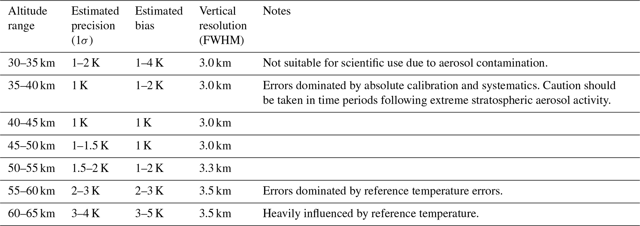
For each retrieved profile the vertical resolution is estimated through fitting of a Gaussian shape to the central peak of the averaging kernel. Generally, mean vertical resolutions are in the range 3.0–3.5 km across the usable retrieval altitudes, which is on the same order as the OSIRIS vertical sampling (2–3 km). A summary of the vertical resolution as a function of altitude is provided in Table 1.

Table 1 Summary of the estimated precision, bias, and vertical resolution of the temperature data product for each altitude range.

4.4 Summary and discussion

All of the assessed sources of error and their quadrature summation are shown in Fig. 10. Bias is dominated by biases in the reference temperature above 45 km and then becomes dominated by errors in the absolute calibration below that. Biases are on the order of 1–4 K depending on the altitude range considered. It should be remembered that the estimated error due to absolute calibration was calculated using an assumed error of 5 % in the absolute radiances, which is only a reasonable estimate. The precision of the retrieval is controlled by random noise below 50 km and then dominated by noise in the reference temperature above that. Precision is typically on the order of 1 K up to 50 km and then increases to 5 K at the highest altitudes. A summary of the estimated precision, bias, vertical resolution, and useful notes to consider for prospective data users is provided in Table 1.

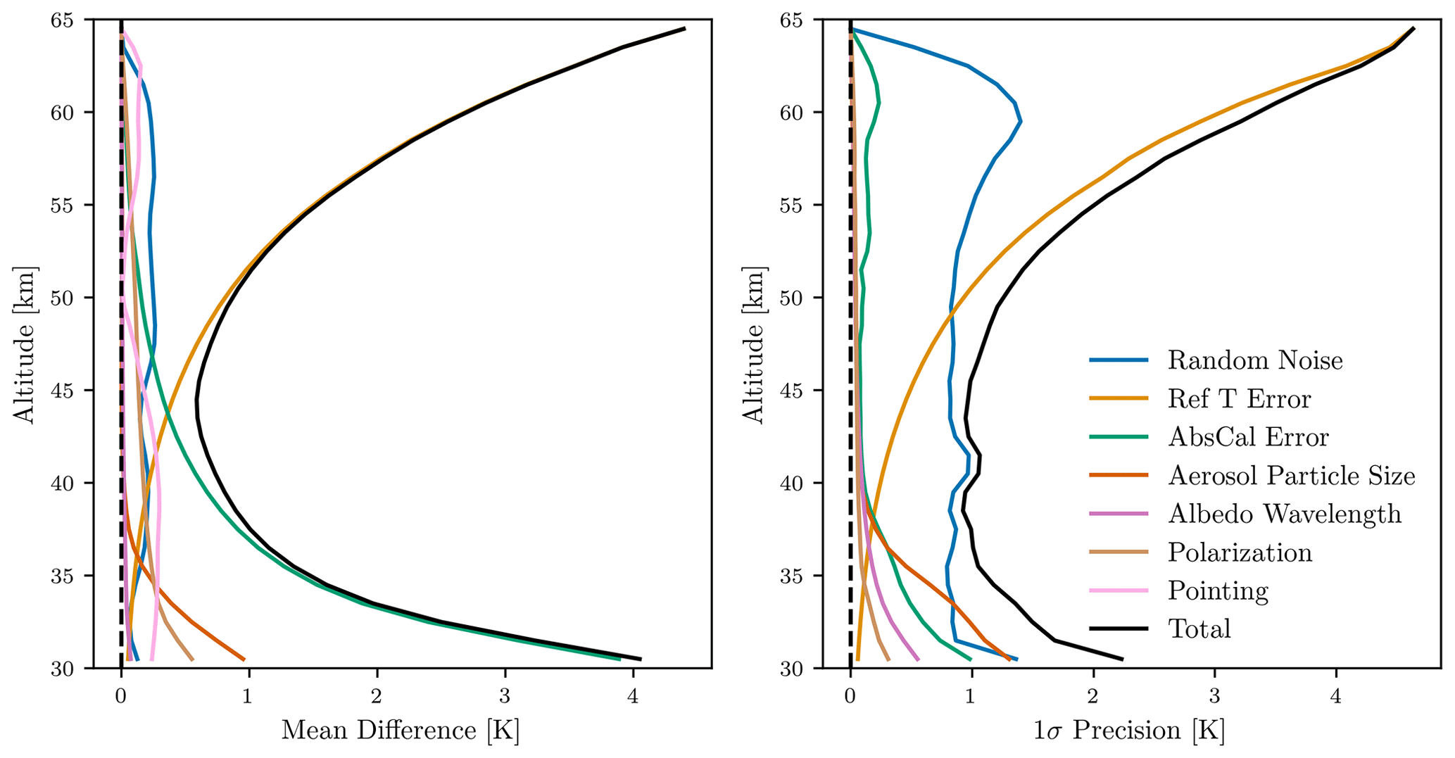
Figure 10 Mean differences and 1σ standard deviation for the 100 test orbits for all perturbation studies performed. See text for details.

So far, the effect of polar mesospheric clouds (PMCs) has not been discussed. PMCs can have a significant impact on the limb scattered radiance signal and can cause extreme variations in the retrieved temperature data product (Chen et al., 2023). Since typical OSIRIS scans terminate at 65 km, well below the nominal altitude of PMCs (80–85 km), accurate detection and filtering of PMCs in OSIRIS data is challenging. Therefore we recommend that use of data in the high latitude summer months be avoided.

5 Comparison with other datasets

5.1 Data descriptions

The retrieved OSIRIS temperatures were validated through comparison with temperature profiles from the Microwave Limb Sounder on Aura (MLS, Waters et al., 2006) and the Atmospheric Chemistry Experiment–Fourier Transform Spectrometer (ACE-FTS, Bernath et al., 2005). All comparisons use the version of the OSIRIS temperatures estimated with MERRA2 as the upper altitude reference value.

MLS observes microwave limb emissions and measures approximately 3500 vertical profiles each day. Temperatures are retrieved near the O₂ spectral lines at 118 and 239 GHz (Livesey et al., 2022). Version 5 of the retrieval is used here and all profiles are filtered according to the guidelines provided in Livesey et al. (2022). The MLS geopotential height (GPH) profiles that are retrieved along with each temperature profile are used to convert the temperature profiles from a vertical pressure grid to a geometric altitude grid before comparing with OSIRIS. Version 5 of the MLS GPH data product matches the 100 hPa surface to input reanalysis data, correcting many systematic issues that were observed with prior versions of the GPH data.

ACE-FTS measures approximately 30 atmospheric transmission profiles each day using a solar occultation geometry: there are ∼ 15 profiles at sunrise and ∼ 15 profiles at sunset. ACE-FTS temperatures are retrieved using observations of CO₂ spectral features in the mid-infrared region. Profiles from version 4.2 of the temperature retrieval, described in Boone et al. (2020), are considered here. The observations are filtered according to the data quality flags developed by Sheese et al. (2015) before being used.

5.2 Coincident comparisons

Coincident profiles between OSIRIS and each MLS and ACE-FTS profile are compared across the January 2005 to December 2023 time period. The coincidence criteria were chosen such that there was a reasonable number of profiles in each of the Northern Hemisphere mid-latitudes, tropics, and Southern Hemisphere mid-latitudes, but without the pairings being too far apart in space and time. For OSIRIS and MLS, the coincident profiles are within 6 h, 2° latitude and 5° longitude. This largely corresponds to comparing OSIRIS, with a local time close to 06:30, to nighttime MLS profiles. For OSIRIS and ACE-FTS the coincident profiles are within 3 h, 5° latitude and 10° longitude. The 3 h time criterion means that only ACE-FTS sunrise profiles are considered.

The mean biases between OSIRIS and MLS temperature profiles in three broad latitude bins are given by the blue lines in Fig. 11, while the mean biases between OSIRIS and ACE-FTS are given by the green lines. In general, OSIRIS and ACE-FTS agree within 3 K at all latitude and altitudes, with OSIRIS biased high compared to ACE-FTS. The differences slightly exceed the predicted systematic biases in Sect. 4.4.

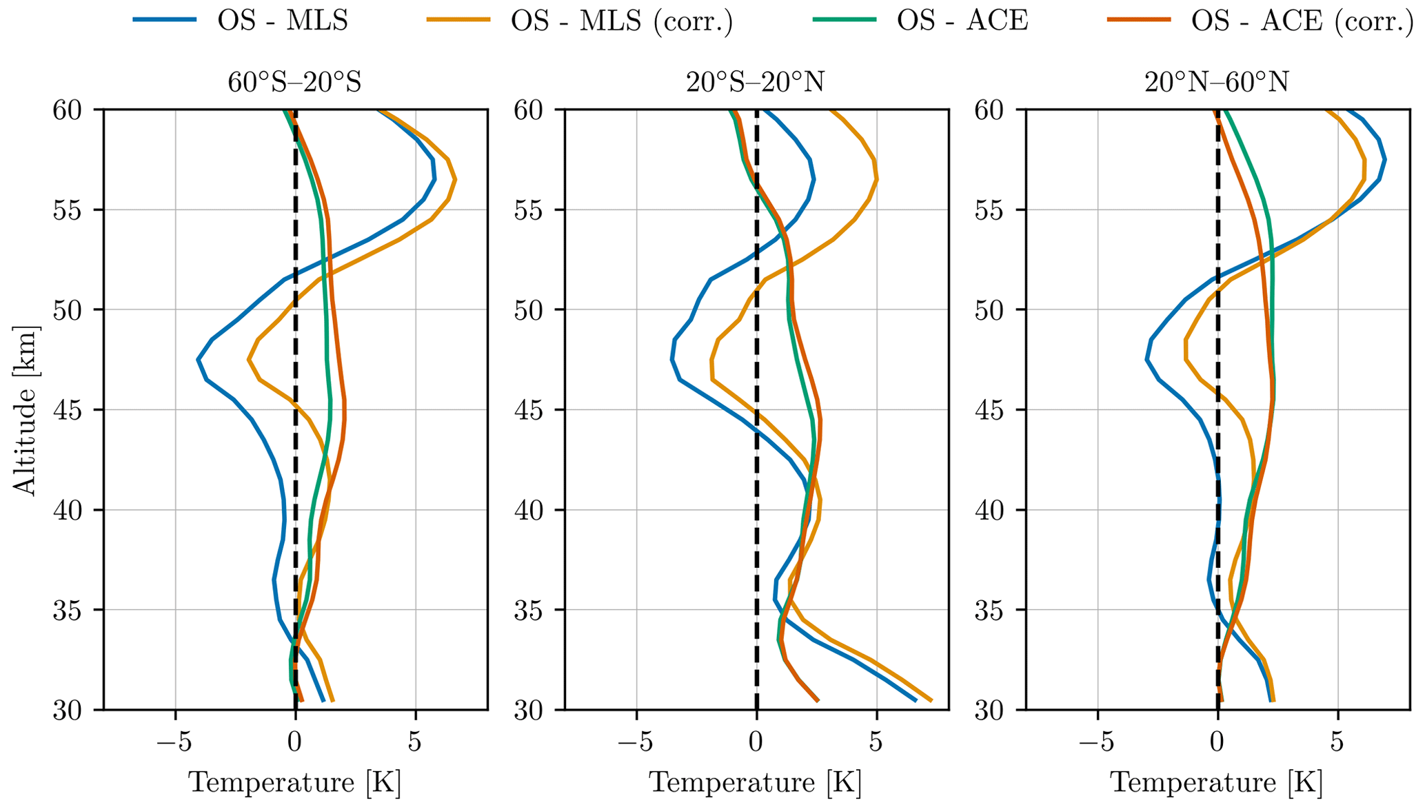
Figure 11 Mean difference between coincident temperature profiles retrieved from OSIRIS, MLS, and ACE-FTS in three latitude bands. Here “corr.” indicates that an estimated diurnal sampling correction has been applied.

MLS and OSIRIS agree within 5 K at all latitudes and altitudes below 55 km. The sign of the bias varies with latitude and altitude. (Schwartz et al., 2008) showed that a previous version of the MLS temperature profiles was biased low by up to 10 K compared to numerous other datasets above 1 hPa. This is likely the main cause of the bias between MLS and OSIRIS above 50 km.

A possible explanation for the observed biases is from the diurnal variation of temperatures, i.e., tidal effects. A correction was performed to assess the impact of the coincident profile sampling on the observed biases. The sampling correction was calculated as the difference between MERRA2 temperatures interpolated to the OSIRIS profile geolocation and MERRA2 temperatures interpolated to the ACE-FTS or MLS geolocation. Since MERRA2 has a 3 h temporal resolution, tidal effects are not well resolved; however, it gives an indication of whether or not the differences are potentially explainable by tides. These results are shown, respectively, by the orange and red lines in Fig. 11. The effect of sampling is at most 1 K for ACE-FTS and 4 K for MLS. Since only ACE-FTS sunrise profiles are used, and OSIRIS usually measures close to sunrise, the effect is generally negligible. For MLS, the sampling effect can be as large as 1–3 K depending on the exact area, suggesting that some of the biases observed between MLS and OSIRIS could be caused by diurnal sampling.

5.3 Seasonal cycle evaluation

The primary driver of longer-scale temperature variations in the middle atmosphere is through the seasonal cycle and thus validation of the seasonal cycle serves as a good test that the retrieval is working as expected. The mean seasonal cycles in temperatures from OSIRIS, MLS, and ACE-FTS are compared in Fig. 12. The structure of the seasonal cycle is broadly similar for each dataset. The greatest difference occurs in the Southern Hemisphere, where MLS and ACE-FTS display colder winter temperatures than those from OSIRIS. The ACE-FTS and MLS temperatures are also slightly colder than those from OSIRIS in the Northern Hemisphere winter. Both of these differences are most likely primarily due to sampling effects where OSIRIS does not uniformly sample the winter hemisphere. In areas where OSIRIS does uniformly sample the latitude band in question, differences rarely exceed 2–4 K.

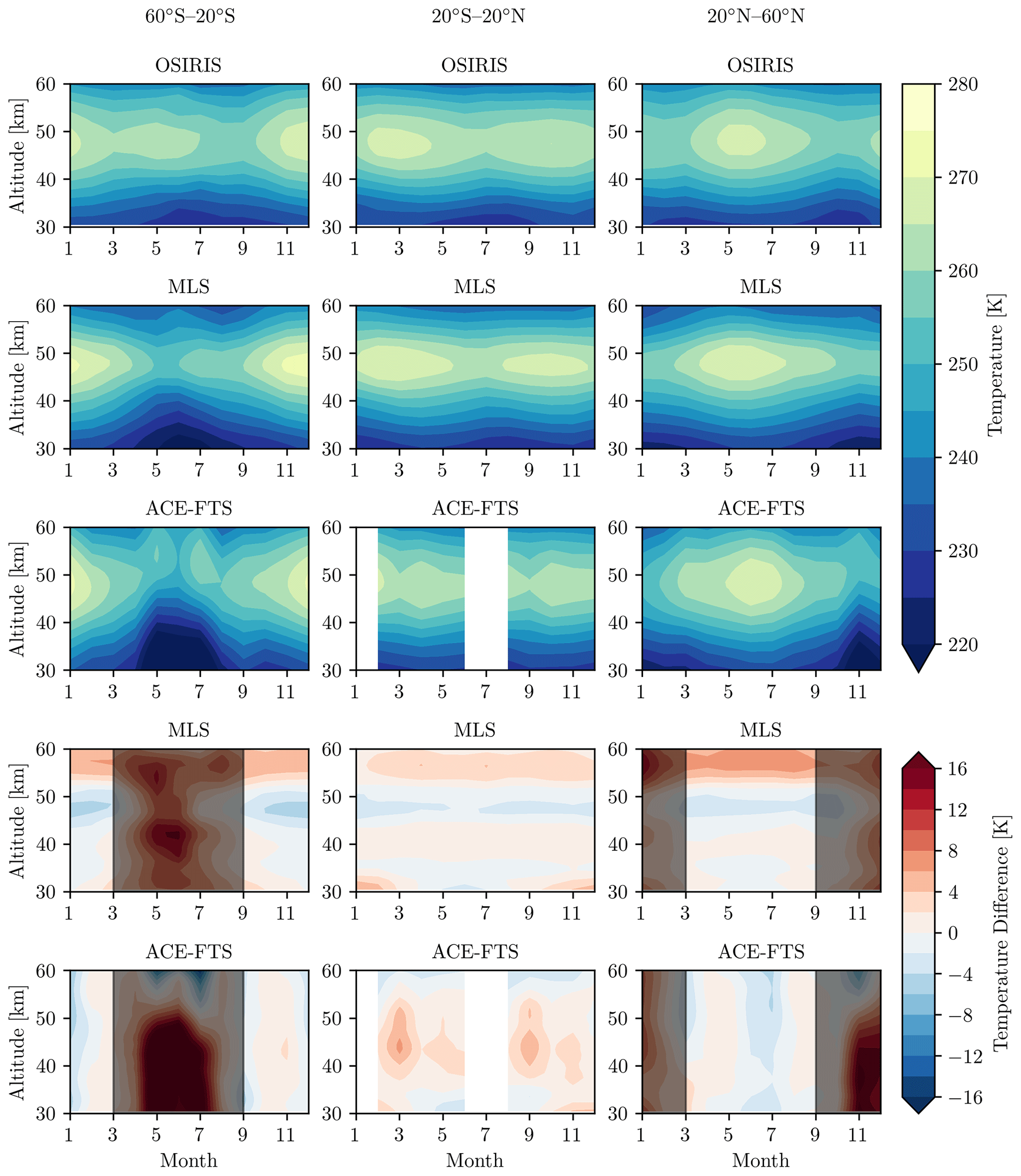
Figure 12 Top three rows: mean seasonal cycle in temperature for OSIRIS, MLS, and ACE-FTS in three latitude bands. Bottom two rows: the difference in seasonal cycle with respect to OSIRIS (OSIRIS – Instrument). Grayed out areas in the difference plots show time periods where OSIRIS does not uniformly sample the specific latitude band.

5.4 Time series comparisons

The de-seasonalized time series for each of the three datasets is shown in Fig. 13. Overall there is very good agreement between the variability of the three datasets at each latitude and altitude. Across all bins, the correlation between MLS and OSIRIS is rarely less than 0.7. Between ACE-FTS and OSIRIS, the correlations are weaker due to the coarse sampling, but are still greater than 0.4 in most bins. There are larger variations in the ACE-FTS temperatures compared to MLS and OSIRIS, particularly in the mid-latitudes, which could be because of the less-dense sampling of ACE-FTS.

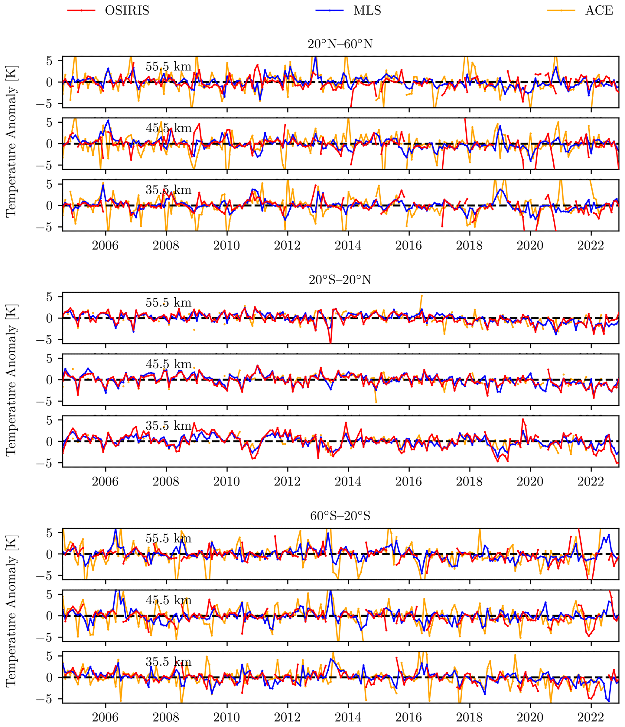
Figure 13 Monthly mean de-seasonalized temperature anomalies for OSIRIS, ACE-FTS, and MLS. Results are provided in three latitude bands and 10 km intervals.

To assess possible drifts in the dataset, in Fig. 14 a linear fit has been performed on the differences in anomalies between OSIRIS and ACE-FTS and between OSIRIS and MLS. For the majority of bins the observed drift between OSIRIS and ACE/MLS is not statistically significant. When there is a statistically significant drift, it is usually less than ±1 K per decade and often does not show up in the same place with respect to ACE/MLS. A consistent cooling greater than 1 K per decade is observed relative to ACE in the middle Southern Hemisphere; however, since it does not show up relative to MLS and ACE, sampling is poor in this latitude band and we expect it is a sampling artifact. In the 45–50 km region at all latitudes a consistent warming is seen relative to MLS that does not appear when compared to ACE-FTS. Given the proximity of this altitude region to the stratopause, it is possible that this is an artifact of the coarse vertical resolution of MLS in this region (∼ 5 km) and the conversion of pressure levels to altitude levels using geopotential height. Overall, with the exception of the 35–42 km region at 60° S, there are no areas of consistent drifts over 1 K per decade between OSIRIS and MLS/ACE. The absence of latitudinally constant drifts at low altitudes suggests that the absolute calibration correction from Sect. 4.3.3 is working as intended.

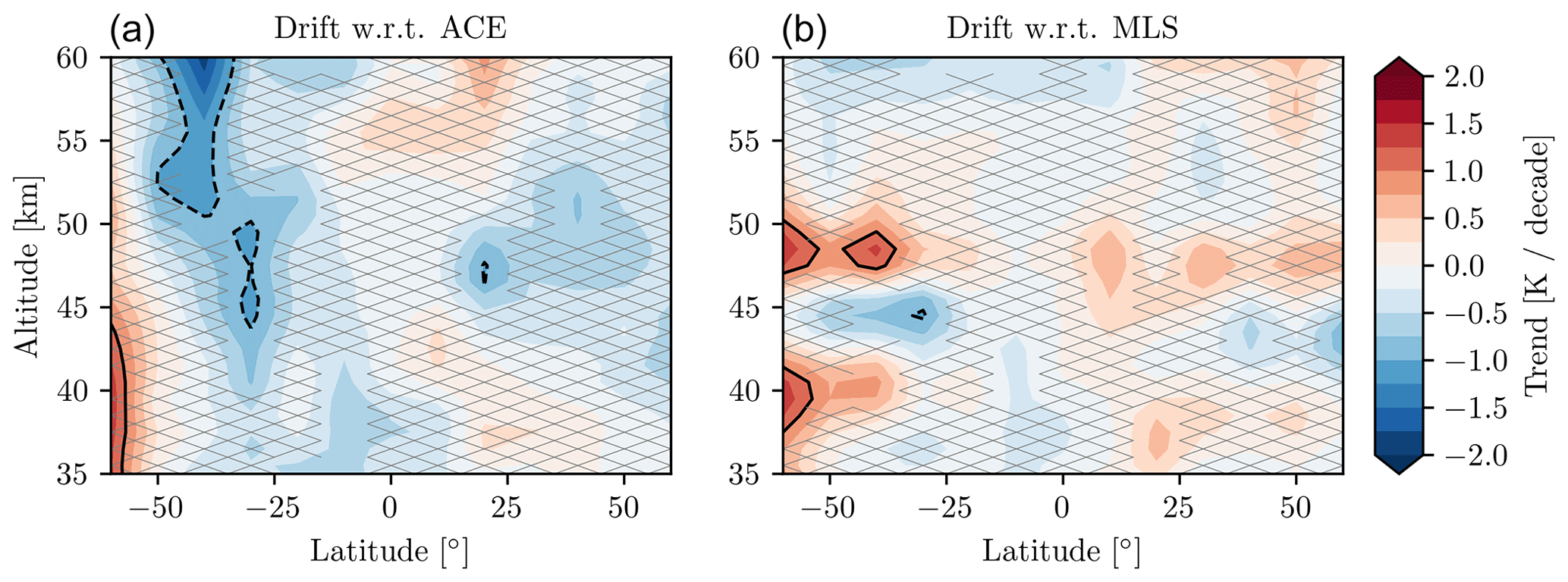
Figure 14 Trend in the difference between monthly mean de-seasonalized temperature anomalies for OSIRIS–ACE (a) and OSIRIS–MLS (b). Trends are calculated using a simple linear fit for the same time period shown in Fig. 13. The 1 and −1 K contours are marked in black. Hatched regions denote a statistically insignificant trend.

6 Conclusions

The method to retrieve atmospheric temperatures with a useful range of 35–60 km included as part of the OSIRIS v7.3 processing has been described. The method combines a retrieval of Rayleigh scattering number density with hydrostatic balance and the ideal gas law to recursively estimate temperature beginning with a reference temperature at a reference high altitude. In contrast to other techniques, multiple scattering is handled directly in the retrieval, with an equivalent Lambertian surface reflectance estimated using an absorbing wavelength. A detailed error analysis has been performed, showing estimated precision to be 1–4 K with potential biases of 1–5 K and a vertical resolution in the range of 3–3.5 km. Errors in the range 45–60 km are dominated by uncertainties in the reference temperature used to pin the solution and errors at altitudes below 45 km are controlled by uncertainties in the absolute calibration of the instrument. An absolute calibration correction has been developed for OSIRIS which greatly reduces drifts in the time series.

Comparisons with temperatures from ACE-FTS and MLS show very good agreement, with biases less than 5 K at most latitudes and altitudes. Seasonal cycles are generally consistent between OSIRIS, MLS, and ACE-FTS, but are challenging to effectively compare because of differences in sampling and local time coverage. Anomaly comparisons between the three instruments show similar variability. Drifts have been assessed between OSIRIS and ACE-FTS/MLS and in most areas they are statistically nonsignificant and rarely exceed 1 K per decade.

Appendix A: Numerical conversion from Rayleigh scattering number density to temperature

The conversion to temperature begins from the equation of hydrostatic balance,

$$\begin{array}{}\text{(A1)}& p\left(z\right)=p\left(z_{\mathrm{0}}\right)-\underset{z_{\mathrm{0}}}{\overset{z}{\int }}g\left(z^{\prime }\right)n\left(z^{\prime }\right)m\left(z^{\prime }\right)\mathrm{d}{z}^{\prime },\end{array}$$

or equivalently,

$$\begin{array}{}\text{(A2)}& p_{i+\mathrm{1}}-p_i=\mathrm{\Delta }{p}_i=-\underset{z_i}{\overset{z_{i+\mathrm{1}}}{\int }}g\left(z^{\prime }\right)n\left(z^{\prime }\right)m\left(z^{\prime }\right)\mathrm{d}{z}^{\prime },\end{array}$$

where the index i=0 represents the top (pinning) altitude, with layers descending vertically, and p is pressure. From this form we can begin with the reference p₀ value and recursively compute the temperature downward through the atmosphere.

To evaluate the integral, we use the fact that SASKTRAN internally performs linear interpolation of the number density between grid points; then, within a single layer the number density is

$$\begin{array}{}\text{(A3)}& n_i\left(z\right)=n_i+{\displaystyle \frac{n_{i+\mathrm{1}}-n_i}{z_{i+\mathrm{1}}-z_i}}(z-z_i).\end{array}$$

We assume the molar mass of air is constant as a function of height and given as 28.97 g mol⁻¹, and that gravitational acceleration decreases quadratically with height according to the relation

$$\begin{array}{}\text{(A4)}& g\left(z\right)=g_{\mathrm{0}}{\displaystyle \frac{R_{\mathrm{e}}^{\mathrm{2}}}{(R_{\mathrm{e}}+z{)}^{\mathrm{2}}}},\end{array}$$

where R_e is the radius of the Earth computed from the average ground track location for each OSIRIS scan, and g₀ is the surface gravitational acceleration. Eq. (A2) can then be rewritten as

$$\begin{array}{}\text{(A5)}& \mathrm{\Delta }{p}_i=-R_{\mathrm{e}}^{\mathrm{2}}m{g}_{\mathrm{0}}\underset{z_i}{\overset{z_{i+\mathrm{1}}}{\int }}{\displaystyle \frac{a_i}{(R_{\mathrm{e}}+z^{\prime }{)}^{\mathrm{2}}}}+{\displaystyle \frac{b_{i}z}{(R_{\mathrm{e}}+z^{\prime }{)}^{\mathrm{2}}}}\mathrm{d}{z}^{\prime },\end{array}$$

with

$$\begin{array}{}\text{(A6)}& a_i=n_i-z_i{\displaystyle \frac{n_{i+\mathrm{1}}-n_i}{z_{i+\mathrm{1}}-z_i}},\end{array}$$

and

$$\begin{array}{}\text{(A7)}& b_i={\displaystyle \frac{n_{i+\mathrm{1}}-n_i}{z_{i+\mathrm{1}}-z_i}}.\end{array}$$

Both integrals can be computed analytically, and the delta pressures between boundaries is a linear function of number density. The absolute pressures at each layer are also a linear function of number density,

$$\begin{array}{}\text{(A8)}& \mathit{p}=p_{\mathrm{0}}+\mathbf{W}\mathit{n},\end{array}$$

where p₀ is pressure at the reference altitude z₀, and W depends only on the Earth radius. Temperature at each grid point can then be evaluated with the ideal gas law,

$$\begin{array}{}\text{(A9)}& T_i={\displaystyle \frac{p_i}{n_{i}k}}.\end{array}$$

The reference pressure is not directly taken from ancillary data, instead it is evaluated using Eq. (A9) with the retrieved number density and the ancillary temperature. The distinction is subtle, but we have found using reference temperature rather than pressure allows for errors in retrieved number density to be canceled more efficiently.

Appendix B: Linear error analysis

The retrieval processor provides an error estimate for the logarithm of number density, ${\widehat{\mathbf{S}}}_{\log n}$, which is calculated through

$$\begin{array}{}\text{(B1)}& \begin{array}{rl}{\widehat{\mathbf{S}}}_{\log n}=& \left[\right({\mathbf{K}}^T{\mathbf{S}}_y^{-\mathrm{1}}\mathbf{K}+{\mathbf{\Gamma }}^T\mathbf{\Gamma }{)}^{-\mathrm{1}}{\mathbf{K}}^T]\\ & {\mathbf{S}}_y\left[\right({\mathbf{K}}^T{\mathbf{S}}_y^{-\mathrm{1}}\mathbf{K}+{\mathbf{\Gamma }}^T\mathbf{\Gamma }{)}^{-\mathrm{1}}{\mathbf{K}}^T{]}^{-\mathrm{1}},\end{array}\end{array}$$

and can be propagated to number density as

$$\begin{array}{}\text{(B2)}& ({\widehat{\mathbf{S}}}_n{)}_{ij}=n_i{n}_j({\widehat{\mathbf{S}}}_{\log n}{)}_{ij}.\end{array}$$

Using Eqs. (A8) and (A9), we can calculate

$$\begin{array}{}\text{(B3)}& {\displaystyle \frac{\partial T_i}{\partial n_j}}={\displaystyle \frac{\mathrm{1}}{n_{i}k}}{W}_{ij}-{\displaystyle \frac{T_i}{n_i}}{\mathit{\delta }}_{ij}.\end{array}$$

The final covariance estimate is then

$$\begin{array}{}\text{(B4)}& {\widehat{\mathbf{S}}}_T=\left[{\displaystyle \frac{\partial T}{\partial n}}\right]{\widehat{\mathbf{S}}}_n{\left[{\displaystyle \frac{\partial T}{\partial n}}\right]}^T.\end{array}$$