Next-generation radiance unfiltering process for the Clouds and the Earth's Radiant Energy System instrument

The filtered radiances measured by the Clouds and the Earth's Radiant Energy System (CERES) instruments are converted to shortwave (SW), longwave (LW), and window unfiltered radiances based on regressions developed from theoretical radiative transfer simulations to relate filtered and unfiltered radiances. This paper describes an update to the existing Edition 4 CERES unfiltering algorithm (Loeb et al., 2001), incorporating the most recent developments in radiative transfer modeling, ancillary input datasets, and increased computational and storage capabilities during the past 20 years. Simulations are performed with the updated Moderate Resolution Atmospheric Transmission (MODTRAN) 5.4 version. Over land and snow, the surface bidirectional reflectance distribution function (BRDF) is characterized by a kernel-based representation in the simulations, instead of the Lambertian surface used in the Edition 4 unfiltering process. Radiance unfiltering is explicitly separated into four seasonally dependent land surface groups based on the spectral radiation similarities of different surface types (defined by the International Geosphere-Biosphere Programme); over snow, it is separated into fresh snow, permanent snow, and sea ice. This differs from the Edition 4 unfiltering process where only one set of regressions was used for land and snow, respectively.

The instantaneous unfiltering errors are estimated with independent test cases generated from radiative transfer simulations in which the “true” unfiltered radiances from radiative transfer simulations are compared with the unfiltered radiances calculated from the regressions. Overall, the relative errors are mostly within ±0.5 % for SW, within ±0.2 % for daytime LW, and within ±0.1 % for nighttime LW for both CERES Terra Flight Model 1 (FM1) and Aqua FM3 instruments. The unfiltered radiances are converted to fluxes and compared to CERES Edition 4 fluxes. The global mean instantaneous fluxes for Aqua FM3 are reduced by 0.34 to 0.45 W m⁻² for SW and increased by 0.25 to 0.46 W m⁻² for daytime LW; for Terra FM1, they are reduced by 0.24 to 0.34 W m⁻² for SW and increased by 0.08 to 0.28 W m⁻² for daytime LW. Nighttime LW flux differences are negligible for both instruments.

1 Introduction

The Clouds and the Earth's Radiant Energy System (CERES) instruments have been continuously monitoring the Earth's radiation budget at the surface, within the atmosphere, and at the top of atmosphere since 2000 (Wielicki et al., 1996). Currently, there are six CERES instruments on board four satellites observing the Earth: Flight Model 1 (FM1) and FM2 on the EOS Terra satellite since 1999; FM3 and FM4 on the Aqua satellite since 2002; FM5 on the Suomi National Polar-orbiting Partnership (SNPP) satellite since 2011; and most recently, FM6 on the NOAA-20 satellite since 2017. CERES instruments measure radiances in shortwave (SW, 0.3–5 µm), window (WN, 8–12 µm), and total (TOT, 0.3–200 µm) channels for FM1–FM5 and SW, TOT, and longwave (LW, 5–40 µm) channels for FM6. The reflected and emitted radiances from Earth scenes enter the instrument aperture, pass through the optical systems, and are recorded by the instrument detectors and electronics (Loeb et al., 2001). However, the measured filtered radiances must be converted to unfiltered radiances which are equivalent to the radiances arriving at the instrument prior to entering its optical system. The unfiltered radiances can be further converted to fluxes with angular distribution models (ADMs; Su et al., 2015) for scientific research (e.g., Sherwood et al., 2020; Loeb et al., 2018).

The radiance unfiltering process in the CERES Edition 4 product uses theoretical radiative transfer simulations to construct regression relationships between filtered and unfiltered radiances (Loeb et al., 2001). If the CERES spectral response functions were spectrally invariant or Earth scenes were spectrally invariant from each other, one set of regression coefficients would be sufficient to convert filtered radiances to unfiltered radiances. However, the spectral response functions are not spectrally flat (Fig. 1) and the spectral distribution of reflected and emitted energy varies with Earth targets (Fig. 2). The radiance unfiltering process must therefore be scene-type dependent. In the CERES Edition 4 radiance unfiltering process, regression coefficients were constructed for land, ocean, and snow/sea ice and further separated into clear and cloudy cases.

Figure 1 Spectral response functions for CERES Terra FM1 and Aqua FM3 instruments.

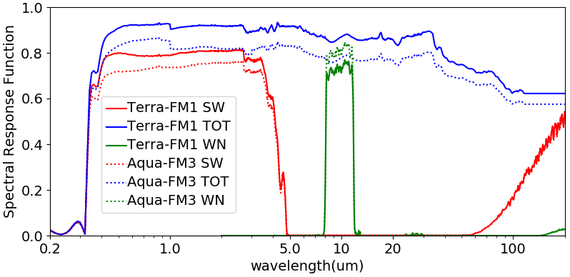
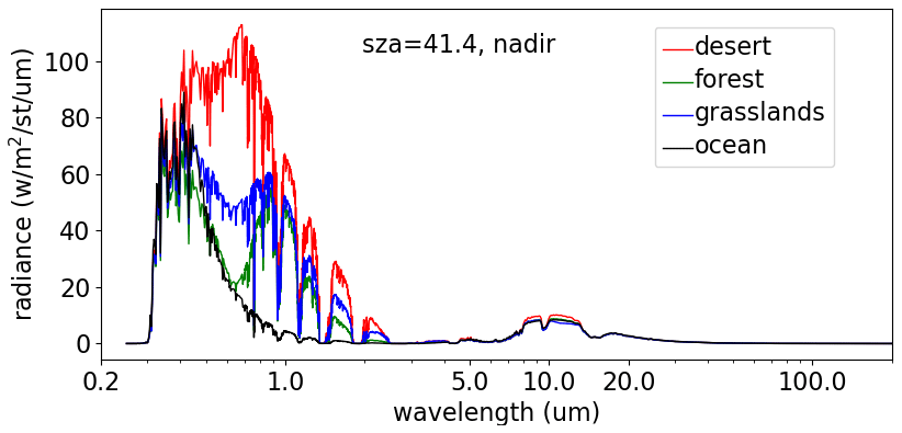
Figure 2 MODTRAN 5.4-simulated clear-sky radiances at the top of atmosphere at SZA of 41.4° over desert, forest, grasslands, and ocean surfaces with surface temperatures of 310, 300, 295, and 290 K, respectively.

A reliable relationship between filtered and unfiltered radiances preferably requires accurate spectral simulations covering a wide range of Earth–atmosphere conditions. With the advances in radiative transfer models, increased computational power and storage, and advances in new observations of Earth–atmosphere during the past 20 years, we are now able to update the CERES radiance unfiltering process. For radiative transfer modeling, Moderate Resolution Atmospheric Transmission (MODTRAN) 3.7 version is replaced by MODTRAN 5.4 with HITRAN database updates for atmospheric gas absorptions and incorporation of discrete-ordinate radiative transfer (DISORT; Stamnes et al., 1988) to calculate multiple scattering faster and with higher fidelity. Over land, the simulations in the Edition 4 radiance unfiltering process used Lambertian surfaces for a limited number of surface types which might not be a sufficient representation of the various land surface types. Furthermore, one set of regression coefficients were developed and applied regardless of the spectral differences among land surfaces. With the advancement of land surface albedo/bidirectional reflectance distribution function (BRDF) observations from the Moderate Resolution Imaging Spectroradiometer (MODIS), we can characterize the surface BRDFs much better than the Lambertian representation in the model simulations. This allows us to identify spectral radiation characteristics among various land surface types, both globally and temporally, upon which the unfiltering coefficients can be developed and applied to more specific land surface types.

To further reduce unfiltered radiance uncertainties, we also use simulations that better match observations to develop the regression coefficients. Over ocean, a better implementation of the Cox–Munk model (Cox and Munk, 1954) is used. Over land, we modify the BRDF kernel parameters from MODIS BRDF/albedo products to better capture the hotspot feature for vegetation (Maignan et al., 2004). Over snow/sea ice, simulations that best match observations are used to develop the regression coefficients for Greenland and Antarctica for permanent snow, sea ice, and fresh snow, respectively. For overcast simulations, we replace the built-in cloud properties in MODTRAN 5.4 with realistic ones.

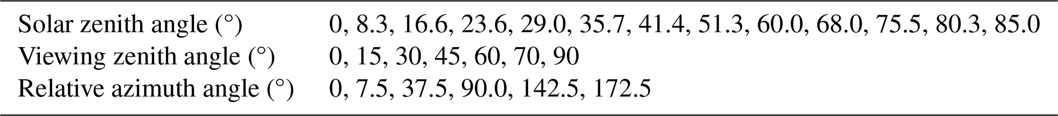
In addition to the above improvements, we increase the number of solar zenith angle (SZA) and viewing zenith angle (VZA) bins at which to calculate the regression coefficients, in order to reduce the unfiltered radiance uncertainties. The number of SZA and VZA bins are increased from 5 to 13 and 5 to 7, respectively, while the number of relative azimuth angle (RAZ) bins remains unchanged at 5 bins.

Section 2.1 of this paper describes the unfiltering algorithm, which is the same as that in Loeb et al. (2001). Detailed radiative transfer simulations are described in Sect. 2.2. Section 3 presents error analysis of the unfiltering process. Section 4 presents applications of the updated radiance unfiltering process to CERES-observed filtered radiances to obtain unfiltered radiances, with which the fluxes are converted for the four seasonal months in 2010.

2 Methodology

2.1 Unfiltering algorithm

The reflected solar and emitted thermal radiances from Earth's surface and atmosphere pass through the optics of CERES instruments. The filtered measurements must be converted to reflect the true reflected and emitted radiances prior to entering CERES instruments. The algorithms were described in detail in Loeb et al. (2001), and a brief description is given below.

The unfiltered reflected shortwave, emitted longwave and window radiances are defined as follows:

$$\begin{array}{}\text{(1a)}& {\displaystyle }{m}_{\mathrm{u}}^{\mathrm{SW}}=\underset{\mathrm{0}}{\overset{\mathrm{\infty }}{\int }}{I}_{\mathit{\lambda }}^{\mathrm{r}}\mathrm{d}\mathit{\lambda }\text{(1b)}& {\displaystyle }{m}_{\mathrm{u}}^{\mathrm{LW}}=\underset{\mathrm{0}}{\overset{\mathrm{\infty }}{\int }}{I}_{\mathit{\lambda }}^{\mathrm{e}}\mathrm{d}\mathit{\lambda }\text{(1c)}& {\displaystyle }{m}_{\mathrm{u}}^{\mathrm{WN}}=\underset{{\mathit{\lambda }}_{\mathrm{1}}}{\overset{{\mathit{\lambda }}_{\mathrm{2}}}{\int }}{I}_{\mathit{\lambda }}^{\mathrm{e}}\mathrm{d}\mathit{\lambda },\end{array}$$

where λ is the wavelength, $I_{\mathit{\lambda }}^{\mathrm{r}}$ and $I_{\mathit{\lambda }}^{\mathrm{e}}$ (W m⁻² sr⁻¹ µm⁻¹) are the reflected solar and emitted thermal radiances, and λ₁ = 8.1 µm and λ₂ = 11.8 µm define a wavelength interval within the thermal window range in CERES FM1–FM5. Given instrument spectral response functions, CERES-measured filtered radiances can be modeled as

$$\begin{array}{}\text{(2)}& m_{\mathrm{f}}^j=\underset{\mathrm{0}}{\overset{\mathrm{\infty }}{\int }}{S}_{\mathit{\lambda }}^j{I}_{\mathit{\lambda }}\mathrm{d}\mathit{\lambda },\end{array}$$

where $S_{\mathit{\lambda }}^j$ is the spectral response function; I_λ is the radiance incident on the instrument; and j denotes the SW, TOT, or WN channel.

For CERES FM1–FM5, the relationships between filtered radiance and unfiltered radiance are constructed through regression as follows:

$$\begin{array}{}\text{(3a)}& {\displaystyle }{m}_{\mathrm{u}}^{\mathrm{SW}}=a_{\mathrm{0}}+a_{\mathrm{1}}{m}_{\mathrm{f}}^{{\mathrm{SW}}_{\mathrm{r}}}+a_{\mathrm{2}}{\left(m_{\mathrm{f}}^{{\mathrm{SW}}_{\mathrm{r}}}\right)}^{\mathrm{2}}\text{(3b)}& {\displaystyle }{m}_{\mathrm{u}}^{\mathrm{WN}}=b_{\mathrm{0}}+b_{\mathrm{1}}{m}_{\mathrm{f}}^{\mathrm{WN}}+b_{\mathrm{2}}{\left(m_{\mathrm{f}}^{\mathrm{WN}}\right)}^{\mathrm{2}}\text{(3c)}& {\displaystyle }{m}_{\mathrm{u}}^{\mathrm{LW}}\left(\mathrm{day}\right)=c_{\mathrm{0}}+c_{\mathrm{1}}{m}_{\mathrm{f}}^{{\mathrm{SW}}_{\mathrm{r}}}+c_{\mathrm{2}}{m}_{\mathrm{f}}^{\mathrm{TOT}}+c_{\mathrm{3}}{m}_{\mathrm{f}}^{\mathrm{WN}}\text{(3d)}& {\displaystyle }{m}_{\mathrm{u}}^{\mathrm{LW}}\left(\mathrm{night}\right)=d_{\mathrm{0}}+d_{\mathrm{1}}{m}_{\mathrm{f}}^{\mathrm{TOT}}+d_{\mathrm{2}}{m}_{\mathrm{f}}^{\mathrm{WN}}.\end{array}$$

For FM6, the window channel is replaced by a LW channel, and the unfiltered LW radiances can be determined by $m_{\mathrm{f}}^{{\mathrm{SW}}_{\mathrm{r}}}$ and $m_{\mathrm{f}}^{\mathrm{TOT}}$ during the daytime and $m_{\mathrm{f}}^{\mathrm{TOT}}$ at night:

$$\begin{array}{}\text{(3e)}& {\displaystyle }{m}_{\mathrm{u}}^{{\mathrm{LW}}_{\mathrm{SW}\mathrm{\_}\mathrm{TOT}}}\left(\mathrm{day}\right)=e_{\mathrm{0}}+e_{\mathrm{1}}{m}_{\mathrm{f}}^{{\mathrm{SW}}_{\mathrm{r}}}+e_{\mathrm{2}}{m}_{\mathrm{f}}^{\mathrm{TOT}}\text{(3f)}& {\displaystyle }{m}_{\mathrm{u}}^{{\mathrm{LW}}_{\mathrm{SW}\mathrm{\_}\mathrm{TOT}}}\left(\mathrm{night}\right)=f_{\mathrm{0}}+f_{\mathrm{1}}{m}_{\mathrm{f}}^{\mathrm{TOT}}.\end{array}$$

The unfiltered LW radiances can also be determined directly from $m_{\mathrm{f}}^{\mathrm{LW}}$:

$$\begin{array}{}\text{(3g)}& m_{\mathrm{u}}^{{\mathrm{LW}}_{\mathrm{LW}}}=g_{\mathrm{0}}+g_{\mathrm{1}}{m}_{\mathrm{f}}^{\mathrm{LW}}+g_{\mathrm{2}}{\left(m_{\mathrm{f}}^{\mathrm{LW}}\right)}^{\mathrm{2}}.\end{array}$$

In Eqs. (3a)–(3g), a₀, a₁, a₂, b₀, b₁, b₂, c₀, c₁, c₂, c₃, d₀, d₁, d₂, e₀, e₁, e₂, f₀, f₁, g₀, g₁, and g₂ are theoretically derived regression coefficients. $m_{\mathrm{f}}^{{\mathrm{SW}}_{\mathrm{r}}}$ is the reflected portion of the filtered SW radiance, and it is determined by removing the emitted thermal portion $m_{\mathrm{f}}^{{\mathrm{SW}}_{\mathrm{e}}}$ from $m_{\mathrm{f}}^{\mathrm{SW}}$:

$$\begin{array}{}\text{(4)}& m_{\mathrm{f}}^{{\mathrm{SW}}_{\mathrm{r}}}=m_{\mathrm{f}}^{\mathrm{SW}}-m_{\mathrm{f}}^{{\mathrm{SW}}_{\mathrm{e}}}.\end{array}$$

For FM1–FM5, $m_{\mathrm{f}}^{{\mathrm{SW}}_{\mathrm{e}}}$ is determined by a relationship between measured $m_{\mathrm{f}}^{\mathrm{SW}}$ and $m_{\mathrm{f}}^{\mathrm{WN}}$ at night:

$$\begin{array}{}\text{(5a)}& m_{\mathrm{f}}^{{\mathrm{SW}}_{\mathrm{e}}}=h_{\mathrm{0}}+h_{\mathrm{1}}{m}_{\mathrm{f}}^{\mathrm{WN}}+h_{\mathrm{2}}{\left(m_{\mathrm{f}}^{\mathrm{WN}}\right)}^{\mathrm{2}}.\end{array}$$

For FM6, $m_{\mathrm{f}}^{{\mathrm{SW}}_{\mathrm{e}}}$ is determined by a relationship between measured $m_{\mathrm{f}}^{\mathrm{SW}}$ and $m_{\mathrm{f}}^{\mathrm{LW}}$ at night:

$$\begin{array}{}\text{(5b)}& m_{\mathrm{f}}^{{\mathrm{SW}}_{\mathrm{e}}}=k_{\mathrm{0}}+k_{\mathrm{1}}{m}_{\mathrm{f}}^{\mathrm{LW}}+k_{\mathrm{2}}{\left(m_{\mathrm{f}}^{\mathrm{LW}}\right)}^{\mathrm{2}}.\end{array}$$

It is useful to emphasize the definitions of the unfiltered SW and LW radiances. In the remainder of the paper, the unfiltered SW radiances are the reflected radiances and the unfiltered LW radiances are the thermal emitted radiances.

2.2 Spectral radiance simulations

2.2.1 Radiative transfer model

The regression coefficients used to convert CERES-observed filtered radiances to unfiltered radiances are developed from radiative transfer simulations over typical Earth scenes. We use MODTRAN 5.4 (Berk et al., 2016) for the radiative transfer simulations, replacing MODTRAN 3.7 in the Edition 4 unfiltering process. A few major improvements in MODTRAN 5.4 as compared to MODTRAN 3.7 include, but are not limited to the following (Berk et al., 2004, 2016):

1. MODTRAN 5.4 is based on HITRAN 2012 (Rothman et al., 2013), while MODTRAN 3.7 is based on HITRAN 1992 (Rothman et al., 1992).

2. MODTRAN 5.4 uses correlated-k algorithm, which significantly improves the accuracy of multiple scattering calculations (Berk et al., 1998).

3. MODTRAN 5.4 allows finer spectral resolution simulations.

4. MODTRAN 5.4 fully treats the auxiliary molecular species.

5. MODTRAN 5.4 calculates multiple scattering faster and with higher fidelity with an improved incorporation of DISORT (Stamnes et al., 1988) into MODTRAN 5.4.

The simulations are performed for clear and overcast conditions, and radiances for broken clouds are linearly weighted with clear-sky and overcast radiances for cloud fractions of 0.25, 0.50, and 0.75. Simulations are performed from 0 to 40 000 wavenumbers per centimeter (0.25 to 1000 µm) with a spectral resolution of 2 wavenumbers per centimeter.

2.2.2 Resolution in the number of angular bins

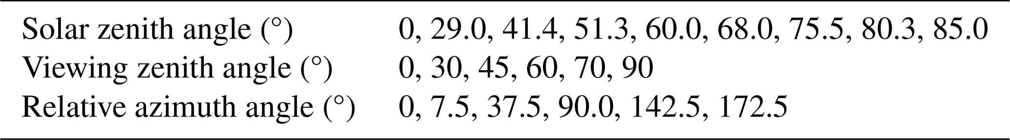
In the Edition 4 unfiltering process, regression coefficients are evaluated at 5 SZA bins, 5 VZA bins, and 5 RAZ bins. The number of SZA bins is increased from 5 to 13, the number of VZA bins is increased from 5 to 7 to minimize the radiance unfiltering uncertainties, and the number of RAZ bins remains the same at 5 bins as in the Edition 4 unfiltering process. The detailed analysis will be shown in Sect. 3. Table 1 shows the SZAs, VZAs, and RAZs at which the radiance unfiltering coefficients are determined for SW, daytime LW, and WN radiances. For nighttime LW and WN radiances, the unfiltering regression coefficients are evaluated at VZA bins only.

Table 1 Regression coefficients angular bin definitions.

2.2.3 Clear-sky simulations over ocean

Over ocean, the surface is characterized by the Cox–Munk model (Cox and Munk, 1954) in the radiative transfer model simulations. The implementation of Takashima (1985) in MODTRAN 3.7 simulations for the Edition 4 CERES radiance unfiltering is replaced by the Second Simulations of a Satellite Signal in the Solar Spectrum (6S) radiative transfer code (Vermote et al., 1997), which includes the radiance contributions from ocean whitecaps and underwater in addition to the specular reflections from the ocean surface. Figure 3 shows that the simulation by the 6S radiative transfer code characterizes the ocean surface radiances better than that of Takashima, particularly for VZAs greater than 50°.

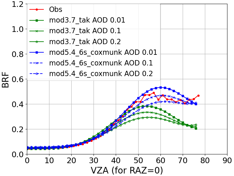
Figure 3 Comparison of CERES Terra FM1-observed unfiltered bidirectional reflectance functions (BRFs) solar principal plane at SZA of 49° to radiative transfer simulations with Cox–Munk ocean surface model (one uses implementation of Takashima (1985) with MODTRAN 3.7 and one uses implementation of the Second Simulation of a Satellite Signal in the Solar Spectrum (6S) radiative transfer code (Vermote et al., 1997) with MODTRAN 5.4) with a wind speed of 5 m s⁻¹ and a tropical profile. Three different aerosol optical depths (AODs) are shown for each model version.

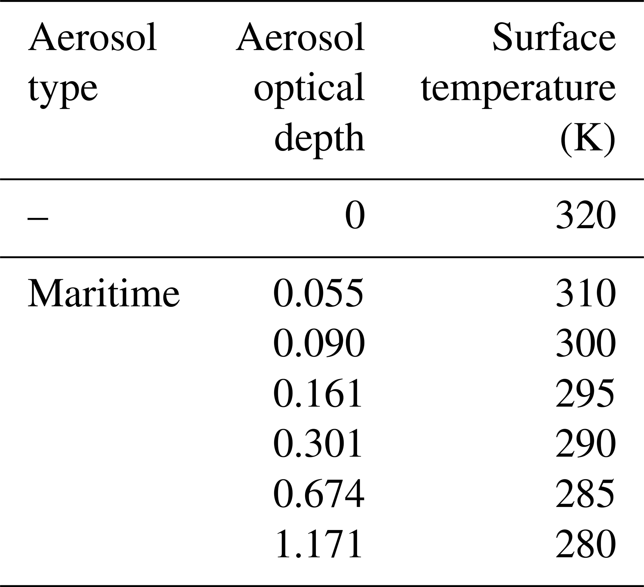
The radiative transfer simulations over clear-sky ocean use the same atmospheric and surface temperature conditions as those in Edition 4 (Table 2). For each solar-viewing angular bin, seven simulations are used to calculate coefficients over clear-sky ocean.

Table 2 Summary of cloud-free properties used in radiative transfer calculations for oceanic conditions with a wind speed of 5 m s⁻¹ and a tropical atmospheric profile.

2.2.4 Clear-sky simulations over land

The radiance unfiltering process is highly scene-dependent, and therefore, it is critical to identify and classify the scene types. In the CERES Edition 4 radiance unfiltering process, regression coefficients were constructed for land, ocean, and snow/sea ice and further separated into clear and cloudy cases. Particularly, over land, Edition 4 used simulations for six land surface types, namely desert, dry sand, vegetation, coniferous forest, forest conifer species, and dry meadows grass (Table 4 in Loeb et al., 2001), from which one set of coefficients was developed for each sun-viewing angular bin regardless of land surface types.

During the last 20 years, we have gained better observations of land surfaces. One of the observations is MODIS-derived land surface albedo/BRDF products. It is based on the semiempirical reciprocal RossThick–LiSparse model (Li and Strahler, 1992; Lucht et al., 2000). The BRF at the surface can be modeled as a linear combination of three terms:

$$\begin{array}{}\text{(6)}& \mathit{\rho }\left({\mathit{\theta }}_{\mathrm{0}},\mathit{\theta },\mathit{\varphi }\right)=f_{\mathrm{iso}}+f_{\mathrm{vol}}{K}_{\mathrm{vol}}\left({\mathit{\theta }}_{\mathrm{0}}\mathit{\theta }\mathit{\varphi }\right)+f_{\mathrm{geo}}{K}_{\mathrm{geo}}\left({\mathit{\theta }}_{\mathrm{0}}\mathit{\theta }\mathit{\varphi }\right),\end{array}$$

where the first term on the right-hand side of the equation is the isotropic-scattering contribution, K_vol in the second term is the RossThick kernel to characterize volumetric scattering from horizontally homogeneous leaf canopies, and K_geo in the third term is the LiSparse kernel to characterize geometrical–optical surface scattering from three-dimensional objects. The kernel fitting parameters f_iso, f_vol, and f_geo were derived from atmospherically corrected, multi-angular land surface BRFs. The derived kernel parameters are available at the seven MODIS spectral bands (0.47, 0.55, 0.65, 0.86, 1.2, 1.6, and 2.1 µm) over a 16 d cycle over land. Validation efforts have shown that the MODIS albedo/BRDF retrievals are in good agreement with field measurements, typically within 10 % (Liang et al., 2002; Jin et al., 2003a, b; Wang et al., 2004).

With the MODIS-derived kernel fitting parameters f_iso, f_vol, and f_geo from albedo/BRDF products for the seven MODIS bands, we are able to estimate the spectral-fitting parameters, which are used to calculate the spectral radiation. The determination of the fitting parameters at other wavelengths across the SW and LW range is described as follows:

1. At wavelengths between 0.47 and 2.1 µm, calculate the fitting parameters with all seven band parameters by the spline interpolation.

2. At wavelengths below 0.47 µm, the fitting parameter f_λ is calculated based on the fitting parameters at 0.47 µm (f_0.47) and 0.55 µm (f_0.55), respectively, along with the spectral reflectances in Jet Propulsion Laboratory (JPL) surface spectral reflectances (Baldridge et al., 2009). Equation (7) shows that one fitting parameter at λ is estimated from f_0.47 by scaling it with R_λ and R_0.47, which are the JPL surface spectral reflectances at λ and 0.47 µm, respectively. Equation (8) shows that another one is estimated from f_0.55 scaled with R_λ and R_0.55 as

   $$\begin{array}{}\text{(7)}& f_{\mathrm{0.47}}^{\mathrm{est}}=f_{\mathrm{0.47}}{\displaystyle \frac{R_{\mathit{\lambda }}}{R_{\mathrm{0.47}}}}\end{array}$$

   and

   $$\begin{array}{}\text{(8)}& f_{\mathrm{0.55}}^{\mathrm{est}}=f_{\mathrm{0.55}}{\displaystyle \frac{R_{\mathit{\lambda }}}{R_{\mathrm{0.55}}}}.\end{array}$$

   The fitting parameter at λ is then calculated as

   $$\begin{array}{}\text{(9)}& \begin{array}{rl}{f}_{\mathit{\lambda }}& =f_{\mathrm{0.47}}^{\mathrm{est}}{\displaystyle \frac{(\mathit{\lambda }-\mathrm{0.55}\mathrm{\mu }\mathrm{m}{)}^{\mathrm{2}}}{(\mathit{\lambda }-\mathrm{0.47}\mathrm{\mu }\mathrm{m}{)}^{\mathrm{2}}+(\mathit{\lambda }-\mathrm{0.55}\mathrm{\mu }\mathrm{m}{)}^{\mathrm{2}}}}\\ & +f_{\mathrm{0.55}}^{\mathrm{est}}{\displaystyle \frac{(\mathit{\lambda }-\mathrm{0.47}\mathrm{\mu }\mathrm{m}{)}^{\mathrm{2}}}{(\mathit{\lambda }-\mathrm{0.47}\mathrm{\mu }\mathrm{m}{)}^{\mathrm{2}}+(\mathit{\lambda }-\mathrm{0.55}\mathrm{\mu }\mathrm{m}{)}^{\mathrm{2}}}};\end{array}\end{array}$$

   that is, we put more weights on $f_{\mathrm{0.47}}^{\mathrm{est}}$ than $f_{\mathrm{0.55}}^{\mathrm{est}}$.

3. The same approach is used to calculate the fitting parameters at wavelengths above 2.11 µm based on the fitting parameters at the 1.6 and 2.1 µm channels.

Figure 4 shows an example comparing SW reflected radiance simulations to CERES-observed SW radiances for evergreen needleleaf forest. It clearly shows that the simulations with MODIS-derived surface BRDF angularly match observations far better than the simulations with a Lambertian surface. However, the simulations based on MODIS-derived surface BRDF still underestimate BRFs around the hotspot angles for vegetated surfaces, where the VZA is equal to the SZA in the backward direction.

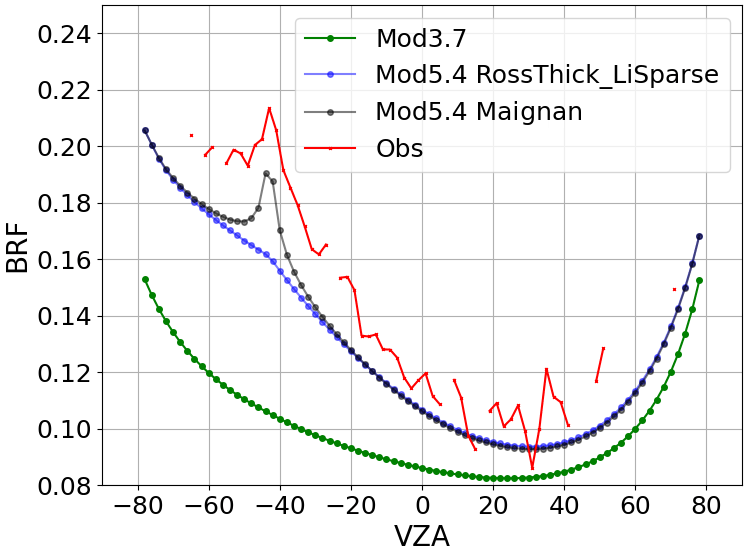
Figure 4 Comparison of MODTRAN simulations to the CERES-observed SW BRFs in the solar principal plane. The CERES observations are over the evergreen needleleaf forest in summer from 2000 to 2020 with SZA in the range of 41 to 43°. MODTRAN 3.7 simulations use Lambertian surface for coniferous forest described in Kriebel (1978). MODTRAN 5.4 simulations use the RossThick–LiSparse model and Maignan-modified RossThick–LiSparse model for the evergreen needleleaf forest with SZA of 43°.

Based on the RossThick–LiSparse model, Maignan et al. (2004) modified K_geo, the geometrical scattering kernel, to highlight the hotspot feature for vegetated surfaces. In the simulations for this version of the radiance unfiltering process, we replaced K_geo for RossThick–LiSparse model with that defined in Maignan et al. (2004). The calculation of new fitting parameters f_iso, f_vol, and f_geo is described as follows:

1. Calculate BRFs at various sun-viewing angles with the MODIS-retrieved fitting parameters for the seven MODIS spectral bands. The calculations are performed with a bin width of 10° for SZA, VZA, and RAZ.

2. With the calculated BRFs in (1), calculate the fitting parameters based on the model described in Maignan et al. (2004) to highlight the hotspot feature of vegetation types. The same model is also implemented in MODTRAN 5.4 to simulate the land surface reflectance.

Figure 4 shows that the simulations with the modified K_geo capture the sharp increases of BRFs around the hotspot angles better than the simulations based on the original RossThick–LiSparse model.

More importantly, based on the spectral simulations with the MODIS-derived kernel fitting parameters, we can identify the radiation spectral characteristics across various land surface types. Figure 5 shows simulations for the 16 land surface types defined by the International Geosphere-Biosphere Programme (IGBP, Table 3) in January. It suggests that the differences in the spectral radiances among different surface types should be considered in the radiance unfiltering process. With a K-means clustering approach, the 16 simulations can be classified into four groups in January based on their radiance spectral similarities. We also found that the grouping is different for other seasons (April, July, and October) compared to January (Table 4). Furthermore, although Fig. 6a indicates that the spectral shapes of evergreen broadleaf forest (IGBP 02) are similar in all four seasons, the spectral shapes of deciduous needleleaf forest (IGBP 03, Fig. 6b) are not, suggesting that we also might need to consider the seasonal variations. To verify the seasonal sensitivity, Fig. 7 shows that the clear-sky SW and daytime LW fluxes over land are substantially different when radiances are unfiltered using unfiltering coefficients developed for January versus those developed for July.

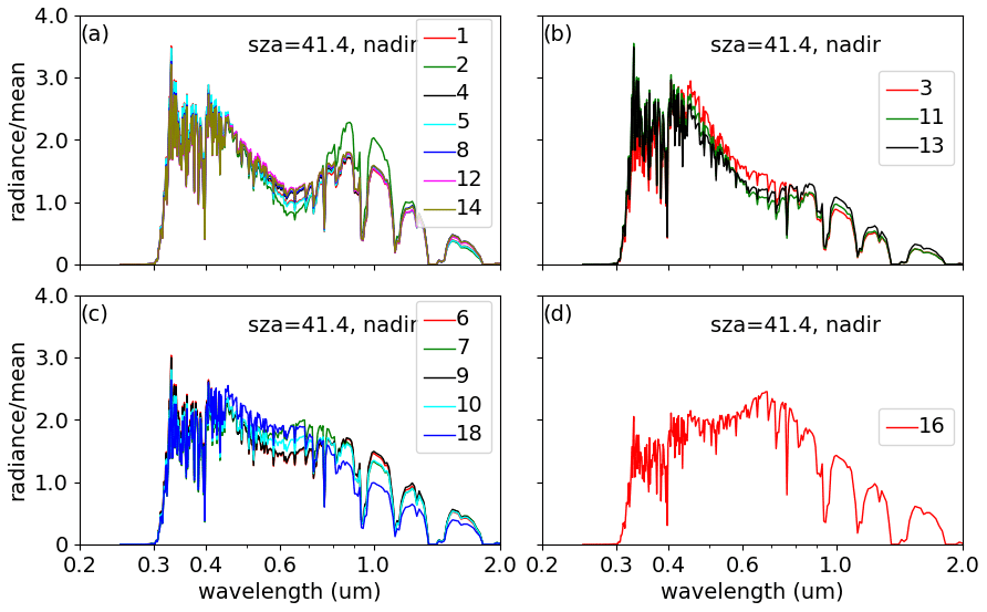
Figure 5 MODTRAN 5.4-simulated clear-sky reflected radiances (normalized by the mean radiance across the spectrum) at the top of atmosphere at SZA of 41.4° in January for 16 land surface types defined by the IGBP.

Table 3 Land surface type indices defined by the International Geosphere-Biosphere Programme (IGBP) and the corresponding names.

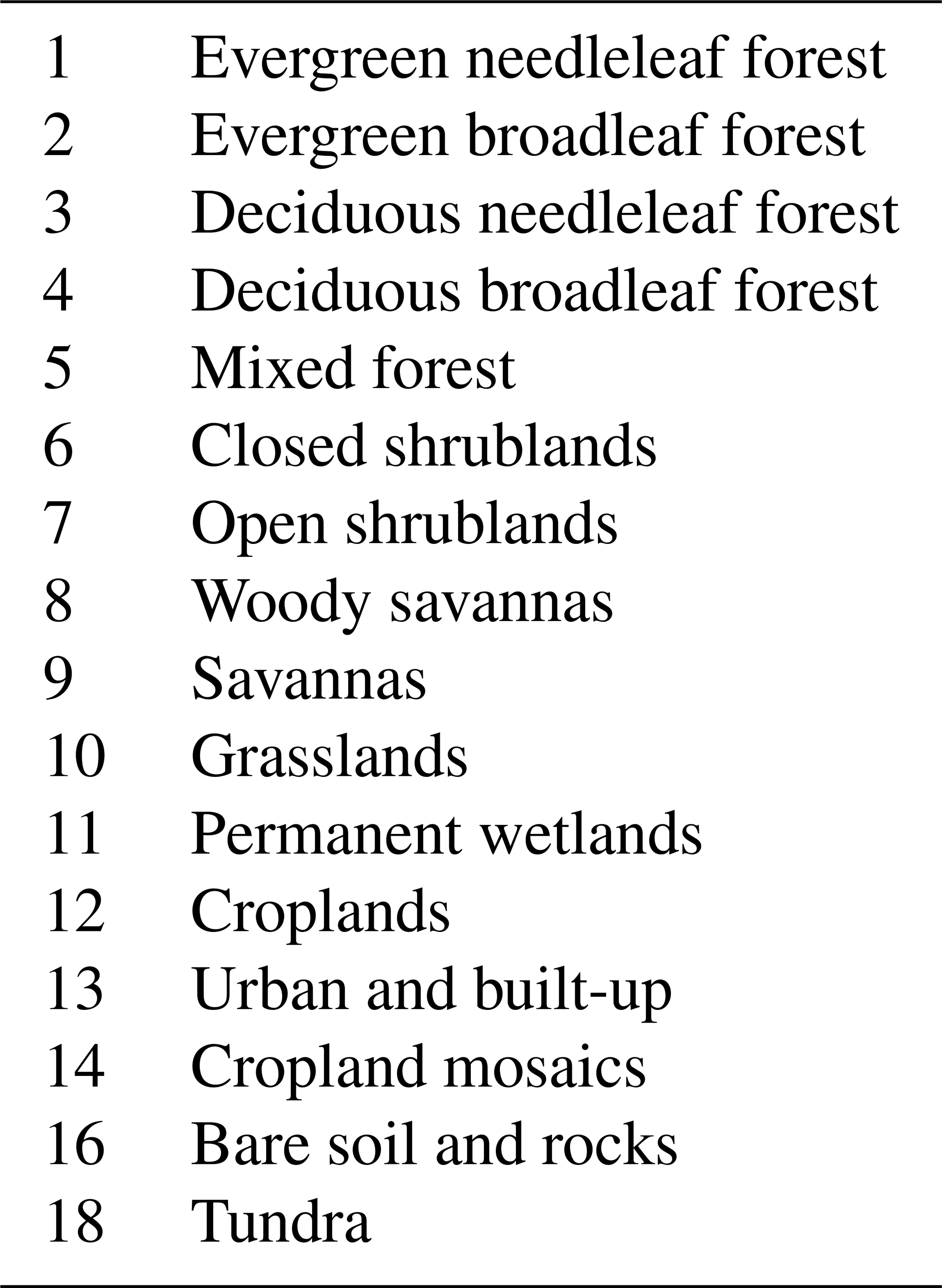
Table 4 Land surface type grouping in January, April, July, and October. The number(s) in a group is (are) IGBP surface type number(s).

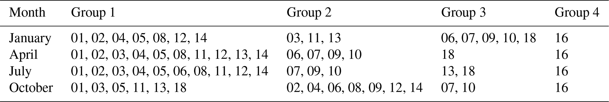
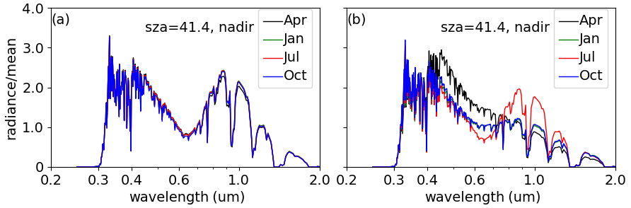
Figure 6 MODTRAN 5.4-simulated clear-sky reflected radiances (normalized by the mean radiance across the spectrum) at the top of atmosphere at SZA of 41.4° for (a) evergreen broadleaf forest (IGBP type 02) and (b) deciduous needleleaf forest (IGBP type 03) in April, January, July, and October.

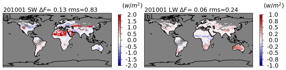
Figure 7 (a) Land clear-sky SW flux differences between fluxes retrieved from the unfiltered radiances based on the unfiltering coefficients for July and those for January. (b) Same as (a) but for daytime LW. Figures show the results for Aqua FM3 in January 2010.

In summary, the radiative transfer simulations over land are performed for each IGBP land surface type based on the 10-year-averaged RossThick–LiSparse model fitting parameters from Collection 6 MODIS-derived albedo/BRDF products MCD43C1 (Strahler et al., 1999; Gao et al., 2005). The unfiltering regression coefficients for land are constructed for four surface groups in each of the four seasons (winter, spring, summer, and fall, respectively). The surface temperatures are prescribed using the median values of a 5-year surface temperature climatology for each IGBP type as calculated from the Goddard Earth Observing System reanalysis (Rienecker et al., 2008), version 5.4.1, included in the Edition 4 CERES Single Satellite Footprint TOA/Surface Fluxes and Clouds (SSF) product data. Depending on the location of a surface type, either a standard, midlatitude summer/winter or subarctic summer/winter atmospheric profile is used. Dust aerosol is used over the bare soil and rocks (IGBP type 16) and open shrublands (IGBP type 07). Rural aerosol is used over other IGBP types. Depending on the surface types, the aerosol optical depths (AODs) use 5, 25, 50, 75, and 95 percentiles of a 5-year AOD climatology from AOD retrieved by MODIS (Collection 5.1), also included in the CERES SSF product. Simulations are also separated for daytime and nighttime with different surface temperatures to account for diurnal temperature variations. For each land surface type, there are 8 to 10 clear-sky cases for each sun-viewing geometry.

2.2.5 Simulations over snow

It is still a challenge to simulate radiation from snow/ice surfaces. In the Edition 4 CERES radiance unfiltering process, the simulations over snow surfaces were characterized by the Warren–Wiscombe model (Wiscombe and Warren, 1980). Compared to CERES observations (Fig. 8), the simulations with the Warren–Wiscombe snow model overestimate BRF for smaller VZAs and underestimate it for larger VZAs, whereas the simulations with the RossThick–LiSparse model are better although they are still unable to match observations at larger VZAs. The unfiltering regression coefficients are developed separately for permanent snow, fresh snow, and sea ice, which contrasts to those in the Edition 4 process, where one set of regression coefficients is used for snow and sea ice. We select the best simulations to match the observations in terms of BRF angular variations in the solar plane to develop regression coefficients to reduce the unfiltered radiance uncertainties as much as possible. The CERES clear-sky observations are compared to simulations based on a 10-year period of MODIS-retrieved BRDF fitting parameters for Greenland and Antarctica using averages in April, July, October, and December and all months. From these 10 simulation candidates, the SW regression coefficients are constructed from two simulations that best match and envelop observed radiances for each snow/sea ice surface. For example, the regression coefficients over Greenland are calculated using simulations based on MODIS BRDF fitting parameters averaged over all months for Greenland and Antarctica, and the regression coefficients over fresh snow are calculated using simulations based on MODIS BRDF fitting parameter averages over Greenland in October and over Antarctica in April. Median values of surface temperature from a 5-year climatology for each snow/sea ice surface are used in the simulations for SW radiance unfiltering. Also from these 10 simulation candidates, the LW and WN regression coefficients are constructed from a simulation that best matches observations along with three surface temperatures which are the 25th, 50th, and 75th percentile values of a 5-year climatology for each snow/sea ice surface. Tropospheric aerosols are used with a visibility of 300 km, and the subarctic winter atmospheric profile is used.

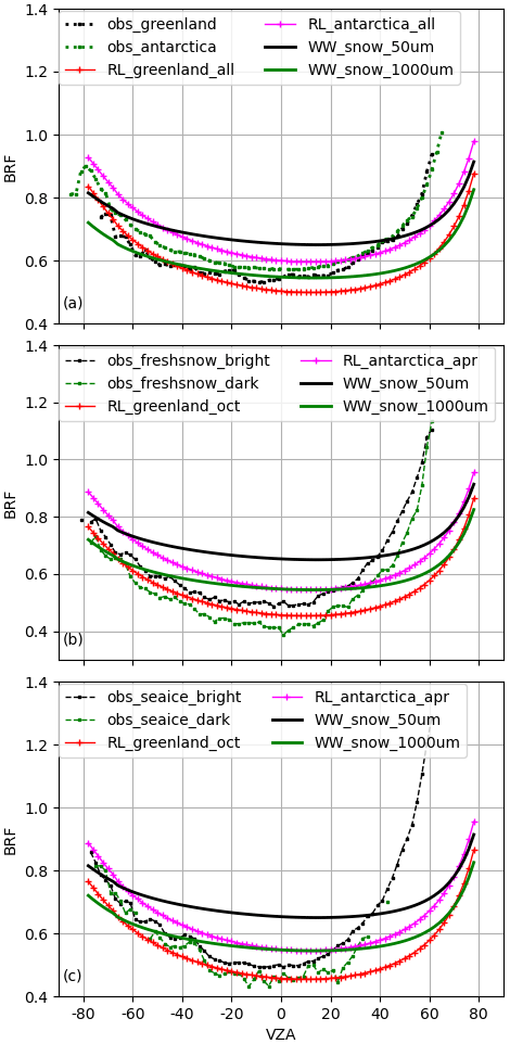
Figure 8 (a) Comparison of MODTRAN 5.4 simulations with surface characterized by Warren–Wiscombe snow model (snow grain size radius of 50 and 1000 µm) and RossThick–LiSparse kernel model to CERES-observed BRFs for permanent snow in the solar principal plane at SZA of 75°. RL_greenland_all (RL_antarctica_all) stands for simulations using the averages of 10-year MODIS-retrieved kernel parameters in all months over Greenland (Antarctica). (b) Same as (a) but for fresh snow; RL_greenland_oct (RL_antarctica_apr) stands for simulations using the averages of 10-year MODIS-retrieved kernel parameters in October over Greenland (Antarctica). Observed fresh snow BRFs are separated into two categories (bright or dark) based on BRF magnitude values in nadir view. (c) Same as (a) but for sea ice.

2.2.6 Simulations for overcast conditions

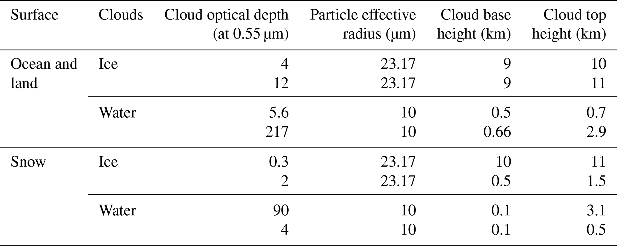
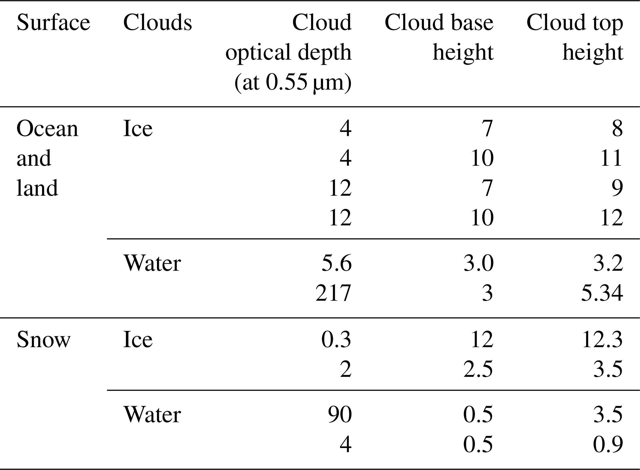
In the Edition 4 radiance unfiltering process, simulations for overcast conditions were performed with built-in cloud optical single-scattering properties in MODTRAN 3.7, such as asymmetry factors, scattering coefficients, and single-scattering albedos. We update them with more realistic cloud optical single-scattering properties to better match the observed radiances. For water clouds, the single-scattering properties, including phase functions, are based on the Mie scattering calculations, and for ice clouds, a two-habit ice cloud model is used (Liu et al., 2014; Loeb et al., 2018). The same models are used in other CERES products, such as cloud property retrievals. A detailed comparison of various ice models can be found in Loeb et al. (2018). For the number of streams for DISORT, an examination of simulated radiances showed that 8 streams for water clouds and 16 streams for ice clouds are sufficient. The overcast properties used in radiative transfer simulations over ocean, land, and snow are shown in Table 5.

Table 5 Summary of overcast properties used in radiative transfer calculations.

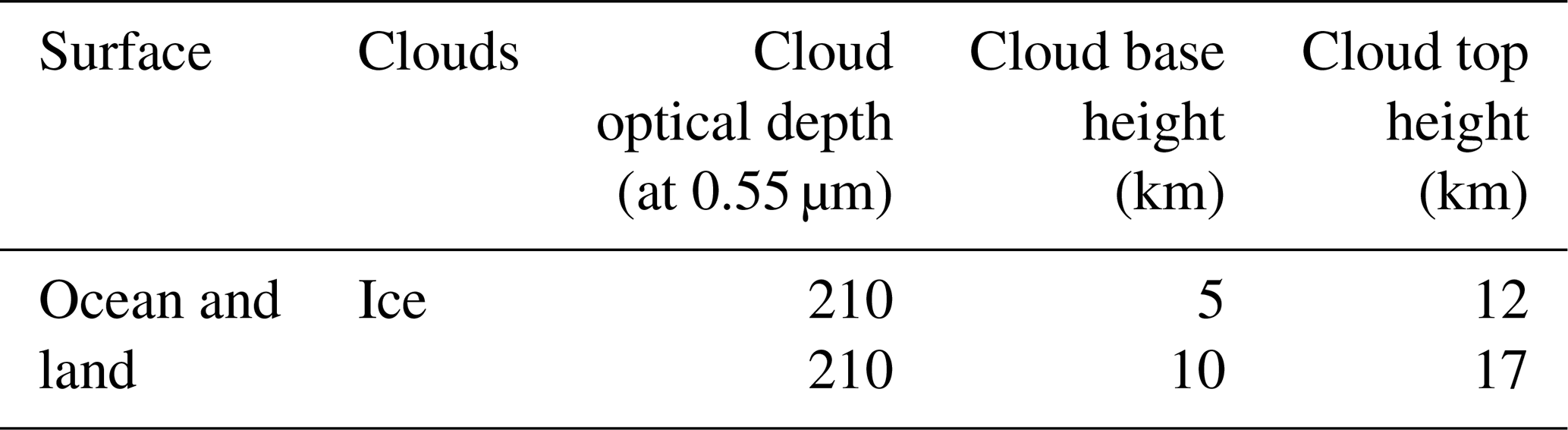
The simulations of deep convective clouds are also included to construct the LW regression coefficients over ocean and land. The conditions used in the deep convective cloud simulation are shown in Table 6.

Table 6 Summary of overcast deep convective cloud properties used in radiative transfer calculations.

2.2.7 Summary of constructed coefficients

To briefly summarize, the regression coefficients are calculated for 13 SZAs, 6 VZAs, and 5 RAZs for SW and daytime LW and 6 VZAs for nighttime LW for each scene type. Scene type is determined by ocean, land (separated into four groups in each of the seasons: spring, summer, fall, and winter), and snow/sea ice (separated into permanent snow over Greenland and Antarctica, fresh snow, and sea ice). Over ocean and land, the coefficients for SW radiance unfiltering are derived separately for clear and cloudy conditions; over snow and sea ice, clear and cloudy scenes use the same coefficients. For LW and WN radiance unfiltering, one set of coefficients is used regardless of cloud coverage conditions. The coefficients derived from both clear and cloudy conditions are used if a scene lacks information of cloud coverage during the application.

3 Error analysis

The instantaneous errors in the unfiltered radiance are estimated by the same approach as used in Loeb et al. (2001). A set of simulations (described in the following sub-sections) that differ from those used to construct the regression coefficients is generated, and it is assumed that they represent the true unfiltered radiances. The simulated radiances are convolved with CERES spectral response functions to obtain filtered radiances. The unfiltering regression coefficients are then applied to the filtered radiances to get unfiltered radiances to compare to the “true” simulated radiances. In the following discussion, without explicitly stating, the errors are evaluated at 9 SZAs, 6 VZAs, and 5 RAZs (Table 7) in the daytime and 6 VZAs and 5 RAZs at nighttime. The error analysis presented is based on CERES Terra FM1. The error analysis for Aqua FM3 can be found in the Supplement (Figs. S1–S8). Given that the errors for unfiltered WN radiances are negligible, only the errors for SW and LW radiances are presented. The unfiltered radiance errors for SNPP FM5 and NOAA20 FM6 are available upon request.

Table 7 Angular bin definitions used to evaluate unfiltered radiance errors.

3.1 Resolution in the number of angular bins

In the Edition 4 radiance unfiltering process, the regression coefficients were evaluated at 5 SZAs, 5 VZAs, and 5 RAZs. The SZAs are 0, 41.4, 60.0, 75.5, and 85.0°. To evaluate if the 5 SZAs are sufficient, we use clear-sky simulations with the same conditions to generate the regression coefficients but at different SZAs: 29, 51.3, 68, and 80.3°. Figure 9 checks if the unfiltered radiance errors at the testing SZAs are comparable to the regression errors for SZAs at 0, 41.4, 60.0, 75.5, and 85.0°. The larger errors in the test cases suggest that the number of SZAs used in Edition 4 is insufficient. In this work, we increase the number of SZAs from 5 to 13 (Table 1). The same approach is used and shows that further increasing the number of SZAs is unnecessary.

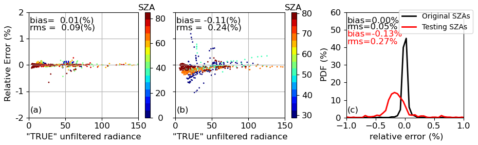
Figure 9 SW unfiltered radiance errors using unfiltering regression coefficients evaluated at 5 SZAs for clear-sky scenes over ocean. (a) Regression errors for SZAs at 0, 41.4, 60.0, 75.5, and 85.0°, at which the regression coefficients are evaluated in the Edition 4 CERES unfiltering process. (b) Errors estimated by alternative SZAs at 29.0, 51.3, 68.0, and 80.3°. (c) Comparisons of the PDFs with data in panels (a) and (b).

With respect to the number of VZAs, we evaluate the unfiltering radiance errors for clear-sky conditions over ocean as the radiances are sensitive to viewing angles. Figure 10a estimates the errors in the solar plane as a function of VZA at SZAs 16.6 and 41.4° based on the regression coefficients evaluated at 6 VZA bins (0, 30, 45, 60, 70, and 90°). It shows that the errors can be quite large for some VZAs. Taking the errors for SZA of 16.6° as an example, the magnitude of errors are 1.0 % with a wind speed of 5 m s⁻¹ and 1.7 % with a wind speed of 12 m s⁻¹ around VZA of 10° in the backward directions. To mitigate these errors, we add a VZA of 15° when developing regression coefficients. Figure 10b shows that the errors are dramatically reduced but the magnitude of the errors can still be greater than 1.0 %. This will be addressed in the future by adding more VZA bins when developing regression coefficients. With respect to the number of RAZs, we verify that 5 RAZs are sufficient.

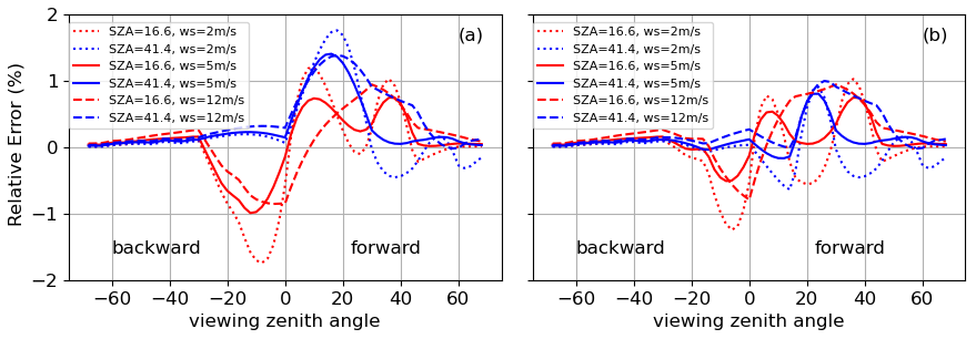
Figure 10 (a) SW unfiltered radiance errors for Terra FM1 in clear-sky scenes over ocean in the solar plane based on the radiance unfiltering coefficients developed for 6 VZA bins (VZA = 0, 30, 45, 60, 70, and 90°). The errors for scenes with wind speeds of 2 and 12 m s⁻¹ are compared to that for simulations with wind speed of 5 m s⁻¹, which is used to construct the regression coefficients for clear-sky scenes over ocean. (b) Same as (a) but for the errors based on the radiance unfiltering coefficients developed for 7 VZA bins (VZA = 0, 15, 30, 45, 60, 70, and 90°).

3.2 Errors due to wind speed over ocean

As mentioned in Sect. 2, the regression coefficients for ocean are generated using radiative transfer simulations with a wind speed of 5 m s⁻¹ and applied to oceanic scenes regardless of wind speed. Figure 11 shows that the SW unfiltered radiance errors for clear-sky scenes with wind speeds of 2 and 12 m s⁻¹ are comparable to the errors of the regression coefficients built with the wind speed of 5 m s⁻¹. Figure 10b further estimates the errors in the solar plane as a function of VZA at two SZAs (16.6 and 41.4°). It shows that for these cases, the magnitude of errors can be close to 1.2 % with a wind speed of 2 m s⁻¹.

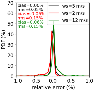
Figure 11 SW unfiltered radiance errors for CERES Terra FM1 in clear-sky scenes over ocean with wind speeds of 2 and 12 m s⁻¹ as compared to those for simulations with a wind speed of 5 m s⁻¹, which is used to construct the regression coefficient for clear-sky scenes over ocean.

3.3 Errors due to aerosols for clear-sky scenes

Over ocean, maritime aerosols are used in radiative transfer simulations to generate regression coefficients (Table 2). We applied these regression coefficients to simulations with different aerosols for clear sky over ocean. Figure 12 shows the SW unfiltered radiance errors for dust and urban aerosols and urban aerosol with larger AOD. Compared to the probability density function (PDF) of SW unfiltered radiance errors for scenes with maritime aerosols, the error PDFs for other aerosols are broader, and the PDF modes for dust and urban aerosols are shifted to negative and positive values, respectively. The mean biases are within ±0.35 %, and RMSEs are below 0.47 %. Over land, Fig. 13 shows the SW unfiltered radiance errors for scenes with larger-AOD aerosols (varying from 0.5 to 2.0 depending on surface type, representing the 99th percentile in AOD climatology for each type) are larger than the scenes used to construct regression coefficients for land. As expected, the magnitude of errors become larger. The mean biases are within ±0.14 %, and RMSEs are below 0.20 %. Overall, errors due to aerosols for most scenes are within ±0.5 %.

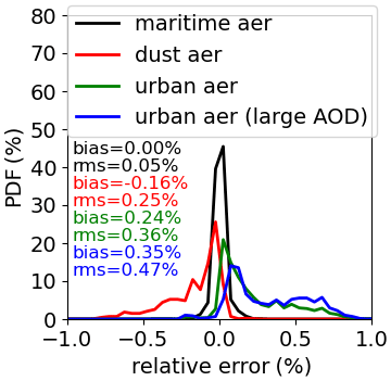
Figure 12 SW unfiltered radiance errors for CERES Terra FM1 in clear-sky ocean scenes with dust, urban, and urban with larger-AOD aerosols as compared to those for simulations with maritime aerosols, which are used to construct regression coefficients for clear-sky scenes over ocean.

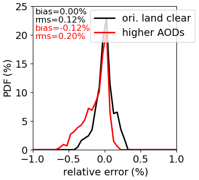
Figure 13 SW unfiltered radiance errors for CERES Terra FM1 in clear-sky land scenes in July with large AODs (varying from 0.5 to 2.0 depending on surface types) as compared to errors in regression coefficients derived from clear-sky land scenes, where AODs used in simulations vary from 0.05 to 0.83 depending on surface type.

3.4 Errors due to scene identification

The CERES radiance unfiltering process is scene-type dependent. Due to cloud mask uncertainties, a clear-sky scene may be mistakenly identified as a cloudy scene, and vice versa. Therefore, an actual clear-sky scene may use regression coefficients for cloudy scenes, and a cloudy scene may use regression coefficients for clear-sky scenes. Taking the simulations to derive the unfiltering regression coefficients of clear-sky scenes over ocean and land in July, Fig. 14 shows that the PDF of SW unfiltered radiance errors for clear-sky scenes unfiltered using the regression coefficients derived from cloudy scenes is wider than those based upon regression coefficients for clear-sky scenes. Overall, the errors are within ±0.5 %. Alternatively, an overcast scene with thin clouds or a broken cloudy scene might be identified as a clear-sky scene. Taking the simulations to derive regression coefficients for cloudy scenes over ocean and land in July, Fig. 15 compares PDFs of SW unfiltered radiance errors for overcast scenes of cirrus with a cloud optical depth (COD) of 2 unfiltered using the regression coefficients derived from clear-sky scenes and cloudy-sky scenes. As expected, the errors for scenes become larger if their corresponding regression coefficients are not used. Most scenes are still within ±0.5 %, although the absolute errors can be as large as 1.0 %. Figure 16 also compares PDFs of radiance errors for broken cloudy scenes with a cloud fraction of 10 % unfiltered using the regression coefficients derived from clear-sky scenes. It shows that the PDFs of radiance errors are comparable with the mean errors near zero and RMSEs are less than 0.18 %.

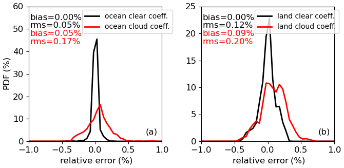
Figure 14 Comparison of SW unfiltered radiance errors for clear-sky scenes unfiltered using the regression coefficients derived from cloudy sky and clear-sky scenes over ocean (a) and land (b) in July for CERES Terra FM1.

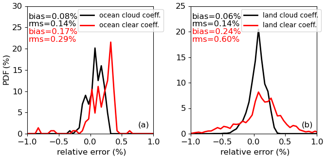
Figure 15 Comparison of SW unfiltered radiance errors for overcast scenes covered by cirrus (COD = 2) unfiltered using the regression coefficients derived from clear-sky scenes and cloudy sky scenes over ocean (a) and land (b) in July for CERES Terra FM1.

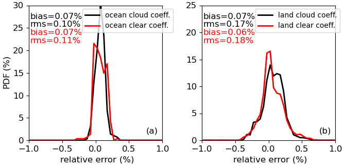
Figure 16 Comparison of SW unfiltered radiance errors for CERES Terra FM1 in broken cloudy-sky scenes (cirrus with COD = 4 and stratus with COD = 5.6 with a cloud fraction of 10 %) unfiltered using the regression coefficients derived from cloudy sky scenes and clear-sky scenes over ocean (a) and land (b) in July.

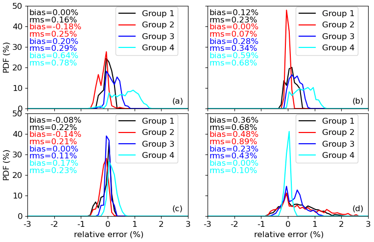
Figure 17 SW unfiltered radiance errors for land surface (a) Group 1, (b) Group 2, (c) Group 3, and (d) Group 4 unfiltered using regression coefficients derived from all four land surface types, respectively, for CERES Terra FM1 in January. In January, Group 1 contains land surface IGBP types 01, 02, 04, 05, 08, 12, and 14; Group 2 contains land IGBP surface types 03, 11, and 13; Group 3 contains land IGBP surface types 06, 07, 09, 10, and 18; and Group 4 contains land IGBP surface type 16.

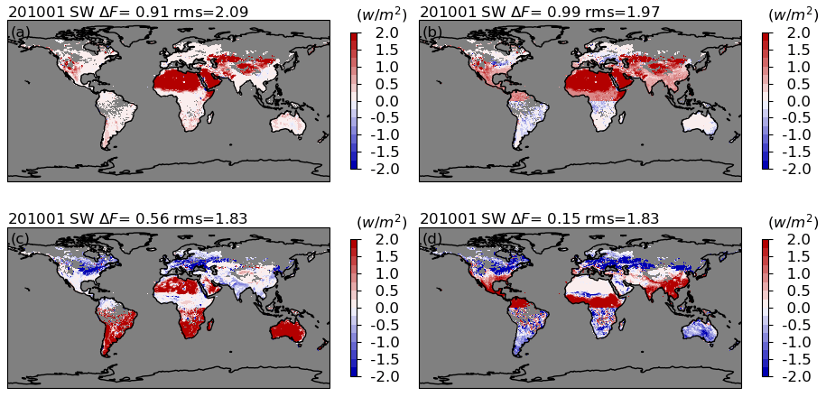
Figure 18 Clear-sky land SW flux differences between fluxes retrieved from the unfiltered radiances using the unfiltering coefficients developed for (a) Group 1, (b) Group 2, (c) Group 3, and (d) Group 4, respectively, and those using corresponding coefficients for each land surface type. Figures show the results for Aqua FM3 in January 2010.

As discussed in Sect. 2, the regression coefficients over land are developed for four land surface groups (defined by IGBP types with similar SW spectral shapes) for each of the four seasons (Fig. 5 and Table 4). Here we further evaluate the SW unfiltered radiance errors for each land surface group unfiltered using the regression coefficients derived from a different land surface group. For example, Fig. 17a shows that the SW unfiltered radiance errors in January for Group 1, which contains land IGBP surface types 01, 02, 04, 05, 08, 12, and 14, caused using the regression coefficients derived from all four groups. As expected, the smallest errors are found when the regression coefficients derived from its group are used. Particularly, the errors for Group 4, which contains IGBP surface type 16, can be up to 2.6 % when the regression coefficients derived from other groups are used. Therefore, it is important to differentiate land surface types when developing the regression coefficients. Figure 18 provides strong evidence that the fluxes change substantially when the regression coefficients developed for a specific group are applied indiscriminately to all land surface types. Consistent with Fig. 17, the largest errors are found over desert regions if the unfiltering coefficients for Group 4 (bare soil and rocks: IGBP surface type 16) are not used (Fig. 18a–c) but the errors are substantially larger for other regions if the unfiltering coefficients for Group 4 are used (Fig. 18d).

3.5 Errors for cloudy scenes

Four cloud properties over land and ocean are used in radiative transfer simulations of overcast scenes to derive regression coefficients for cloudy scenes (Table 5). One of the simulations represents stratus overcast scenes with a COD of 5.6. Simulations with the same conditions but using a different COD of 38 are used to evaluate the SW unfiltered radiance errors. Another simulation represents cirrus overcast scenes with a COD of 4. Simulations with the same conditions but with a COD of 1 are used to evaluate the errors. Figure 19 shows that the errors for stratus are similar, while the error PDF for cirrus with COD of 1 is broader than those with a COD of 4 but the errors are still within 0.5 %.

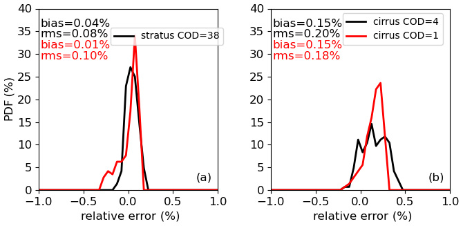
Figure 19 (a) SW unfiltered radiance errors for CERES Terra FM1 in cloudy sky scenes covered by stratus with COD of 38 as compared to those covered by stratus with COD of 5.6 unfiltered using regression coefficients derived from cloudy sky scenes over ocean. (b) Same as (a) but for comparing the errors for cirrus clouds with CODs of 1 and 4.

3.6 Errors due to surface and cloud top temperatures

As mentioned in Sect. 2, to derive regression coefficients for LW, the surface temperatures varying from 280 to 320 K over ocean are used in simulations. Over land, the median values of surface temperature in 5-year climatologies are used, and over snow/sea ice, the 25th, 50th, and 75th percentiles of the surface temperatures are used. For clear-sky conditions, we use simulations with the minimum and maximum surface temperatures from climatologies, keeping all other conditions the same to evaluate the unfiltered LW radiance error. For overcast conditions, the unfiltered radiance errors are evaluated from simulations with clouds placed at different altitudes (Table 8) as compared to those used to generate the regression coefficients (Table 5). Both tests show that the errors are within 0.1 %.

Table 8 Summary of overcast properties used in radiative transfer calculations over ocean and land for the LW unfiltered radiance error analysis.

4 Impact of unfiltering algorithm on instantaneous fluxes

The newly updated regression coefficients are applied to the filtered radiances to obtain the unfiltered SW, LW, and WN radiances of CERES Terra FM1 and Aqua FM3 instruments. With CERES Edition 4 ADMs (Su et al., 2015), the unfiltered radiances are converted to corresponding instantaneous fluxes. Figures 20–24 show the SW, daytime, and nighttime LW flux differences between the newly calculated fluxes and the CERES Edition 4 fluxes for Aqua FM3 in January, April, July, and October in 2010 (the corresponding analyses for Terra FM1 are shown in Figs. S9 to S13).

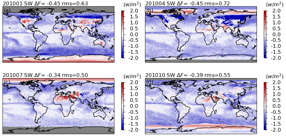
Figure 20 The differences between the SW instantaneous fluxes retrieved with unfiltered radiances based on the updated CERES radiance unfiltering process and that based on the unfiltered radiances in the CERES Edition 4 product for the CERES Aqua FM3 instrument in January (a), April (b), July (c), and October (d).

Figure 21 Same as Fig. 20 but for the relative differences.

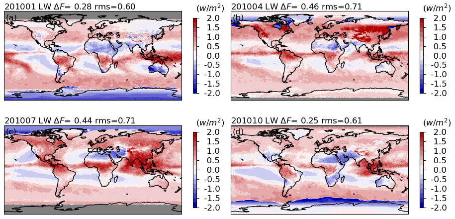
Figure 22 Same as Fig. 20 but for daytime LW.

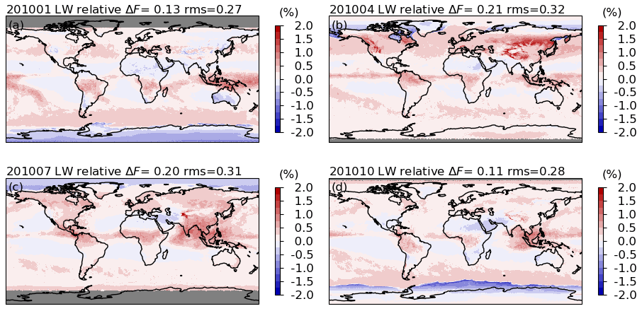
Figure 23 Same as Fig. 22 but for the relative differences.

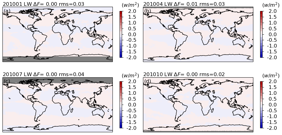
Figure 24 Same as Fig. 20 but for nighttime LW.

For SW fluxes (Figs. 20 and 21) over ocean, the difference pattern correlates with the cloud coverage distribution. Negative-value regions covered with high clouds can be associated with the changes in the cloud microphysical properties used in MODTRAN simulations (Sect. 2.2.6), while the new implementation of the Cox–Munk ocean model has less of an impact on clear-sky conditions over ocean. Over land, SW flux differences are geographically dependent, as expected, which further justifies the development of a surface-type-dependent unfiltering process. The SW flux differences vary seasonally, supporting the need for seasonal stratification in the unfiltering process. The fluxes decrease in January and increase in July over desert regions, while the flux changes over vegetation-covered regions are relatively small. In January and April over the middle to high latitudes in the Northern Hemisphere, the large negative values are associated with surfaces covered by fresh snow. In all months, positive values are found over permanent snow and sea ice (except sea ice in April). Both should be due to the changes in the snow/ice model in the simulations (Sect. 2.2.5). Given that the new simulations over snow or sea ice are better than those used in Edition 4 (Sect. 2.2.5), we believe that the new process should be more realistic, even though the simulations over snow or sea ice are still far from closely matching the observations (Fig. 8). Quantitatively, the SW global mean instantaneous fluxes for Aqua FM3 are reduced by 0.34 to 0.45 W m⁻², and there are 4.0 %, 0.9 %, 0.4 %, and 2.5 % of 1° × 1° grids in January, April, July, and October in 2010, respectively, that have differences with a magnitude greater than 2.0 W m⁻². In terms of the relative differences, the fluxes are reduced by 0.06 % to 0.20 %. For Terra FM1 (Figs. S9 and S10), the global mean instantaneous flux is reduced by 0.24 to 0.34 W m⁻² with the differences showing similar regional patterns as Aqua FM3 but with smaller magnitudes.

The daytime LW flux differences also show regional dependences (Figs. 22 and 23). The locations of positive LW flux differences correspond to locations of negative SW flux differences and vice versa. Given that the nighttime LW flux differences (Fig. 24) are nearly negligible (with a ∼ 0 W m⁻² global mean and less than 0.04 W m⁻² root mean square error), the correlations are largely due to the subtraction of the SW component from the TOT radiances. In other words, the daytime LW radiance unfiltering is critically related to the performance of the SW radiance unfiltering process. Quantitatively, the global mean instantaneous fluxes are increased by 0.25 to 0.46 W m⁻² for Aqua FM3, and there are 0.2 %, 1.5 %, 0.5 %, and 0.8 % of 1° × 1° grids in January, April, July, and October in 2010, respectively, that have differences with a magnitude greater than 2.0 W m⁻². In terms of the relative differences, the fluxes are increased by 0.03 % to 0.11 %. For Terra FM1, the global mean fluxes are increased by 0.08 to 0.28 W m⁻² (Figs. S11 and S12).

5 Summary

CERES instruments measure filtered reflected solar and emitted thermal infrared radiances from the Earth–atmosphere system. For use in science applications, the filtered radiances must be converted to unfiltered radiances, which are equivalent to the radiances arriving at the instrument prior to entering its optical system. The unfiltered radiances are then converted to radiative fluxes for scientific research. This paper describes an update to the existing Edition 4 CERES unfiltering algorithm (Loeb et al., 2001) by incorporating the most recent developments in radiative transfer modeling, ancillary input datasets, and increased computational and storage capabilities during the past 20 years. A few of the improvements in the new version are as follows:

1. Simulations are performed with MODTRAN 5.4 with many updates as compared to MODTRAN 3.7, such as a newer HITRAN dataset, adopting the correlated-K algorithm to calculate absorptions, allowing finer spectral resolution, and an improved incorporation of DISORT to calculate multiple scattering radiations (Berk et al., 2004, 2016).

2. Over ocean, the implementation of the Cox–Munk BRDF model in the 6S radiative transfer code replaces the implementation in Takashima (1985) used in simulations for the Edition 4 radiance unfiltering process. The newer version matches the CERES-observed angular variation of the SW radiances better.

3. For simulations over land and snow, surface BRDFs are characterized by MODIS-retrieved RossThick–LiSparse kernel-based BRDF model fitting parameters for each IGBP surface type, instead of the Lambertian surface used in simulations for the Edition 4 CERES radiance process. The hotspot features for vegetation are further modeled using the approach described in Maignan et al. (2004).

4. Over land, unfiltering regression coefficients are derived separately into four surface groups to characterize spectral differences among different surface types. The regression coefficients are also separated into four seasons to characterize the seasonal variation of the surfaces.

5. The regression coefficients are calculated at more SZA bins, increased to 13 from 5 in SZA as used in Edition 4, to reduce the unfiltered radiance errors.

6. Climatological surface temperatures from Goddard Earth Observing System reanalysis were used in simulations over land, snow, and sea ice. Climatological AODs derived from MODIS over land are also used in the simulations.

Instantaneous unfiltered radiance errors were estimated using radiative transfer simulations. The simulated filtered radiances are converted to unfiltered radiances and compared to the simulated unfiltered radiances. Overall, the instantaneous relative errors are mostly within ±0.5 % for SW radiances, within ±0.2 % for daytime LW radiances, and negligible for nighttime LW and WN radiances. However, the errors are larger for some extreme cases, such as very large AODs for clear-sky and misclassified cloudy or clear-sky scenes and for scenes with radiances that are very sensitive to the sun-viewing geometry.

The unfiltered radiances with the newly updated unfiltering regression coefficients are converted to fluxes and compared to fluxes in Edition 4. The global mean instantaneous fluxes for Aqua FM3 are reduced by 0.34 to 0.45 W m⁻² for SW and are increased by 0.25 to 0.46 W m⁻² for daytime LW; while for Terra FM1, the global mean instantaneous fluxes are reduced by 0.24 to 0.34 W m⁻² for SW and increased by 0.08 to 0.28 W m⁻² for daytime LW, though the regional differences can be greater than 2.0 W m⁻². For nighttime LW fluxes, the differences are negligible for both instruments.

The instantaneous unfiltered radiance errors for CERES SNPP FM5 and NOAA20 FM6 are similar to those of Terra FM1 and Aqua FM3 (not shown). As for the regional distribution of flux differences, NOAA20 FM6 is similar to Terra FM1 and Aqua FM3 but with a smaller magnitude of differences. However, while the regional SW fluxes are mostly reduced (Figs. 20 and 21) and daytime LW fluxes are increased (Figs. 22 and 23) for Aqua FM3, the regional SW fluxes are mostly increased and daytime LW fluxes are decreased for SNPP FM5, both to a lesser degree than Terra FM1 or Aqua FM3 (Figs. S13 and 14). Further investigations are needed to determine how the spectral response functions impact the unfiltering process to respond to these changes.