the Creative Commons Attribution 4.0 License.
the Creative Commons Attribution 4.0 License.
 | 18 Apr 2024
Greenhouse gas retrievals for the CO2M mission using the FOCAL method: first performance estimates
Stefan Noël
Michael Buchwitz
Michael Hilker
Maximilian Reuter
Michael Weimer
Heinrich Bovensmann
John P. Burrows
Hartmut Bösch
Ruediger Lang
The Anthropogenic Carbon Dioxide Monitoring (CO2M) mission is a constellation of satellites currently planned to be launched in 2026. CO2M is planned to be a core component of a Monitoring and Verification Support (MVS) service capacity under development as part of the Copernicus Atmosphere Monitoring Service (CAMS). The CO2M radiance measurements will be used to retrieve column-averaged dry-air mole fractions of atmospheric carbon dioxide (XCO2), methane (XCH4) and total columns of nitrogen dioxide (NO2). Using appropriate inverse modelling, the atmospheric greenhouse gas (GHG) observations will be used to derive United Nations Framework Convention on Climate Change (UNFCCC) COP 21 Paris Agreement relevant information on GHG sources and sinks. This challenging application requires highly accurate XCO2 and XCH4 retrievals. Three different retrieval algorithms to derive XCO2 and XCH4 are currently under development for the operational processing system at EUMETSAT. One of these algorithms uses the heritage of the FOCAL (Fast atmOspheric traCe gAs retrievaL) method, which has already successfully been applied to measurements from other satellites. Here, we show recent results generated using the CO2M version of FOCAL, called FOCAL-CO2M.
To assess the quality of the FOCAL-CO2M retrievals, a large set of representative simulated radiance spectra has been generated using the radiative transfer model SCIATRAN. These simulations consider the planned viewing geometry of the CO2 instrument and corresponding geophysical scene data (including different types of aerosols and varying surface properties), which were taken from model data for the year 2015. We consider instrument noise and systematic errors caused by the retrieval method but have not considered additional error sources due to, for example, instrumental issues, spectroscopy or meteorology. On the other hand, we have also not taken advantage in this study of CO2M's MAP (multi-angle polarimeter) instrument, which will provide additional information on aerosols and cirrus clouds. By application of the FOCAL retrieval to these simulated data, confidence is gained that the FOCAL method is able to fulfil the challenging requirements for systematic errors for the CO2M mission (spatio-temporal bias ≤ 0.5 ppm for XCO2 and ≤ 5 ppb for XCH4).
- Article
(15371 KB) - Full-text XML
- BibTeX
- EndNote


Carbon dioxide (CO2) and methane (CH4) are the two most important anthropogenic atmospheric greenhouse gases. Their atmospheric concentrations are rising as a result of anthropogenic activity. There is a scientific consensus that this is driving global warming and related climate change (see the recent report of the Intergovernmental Panel on Climate Change (IPCC) 2023). In November 2015, the Paris Agreement of the United Nations Framework Convention on Climate Change (UNFCCC) was adopted to limit global warming to well below 2 °C (UNFCCC, 2015). Actually, this treaty introduced a preferred limit of 1.5 °C. As part of the Paris Agreement, progress of emission reduction efforts is tracked on a regular basis. In this context, the European Commission (EC), the European Space Agency (ESA), the European Centre for Medium-Range Weather Forecasts (ECMWF), the European Organisation for the Exploitation of Meteorological Satellites (EUMETSAT) and international experts are developing an operational capacity for monitoring anthropogenic CO2 emissions as a new CO2 service under the EC's Copernicus programme (e.g. Janssens-Maenhout et al., 2020; Balsamo et al., 2021). A core component of this Monitoring and Verification Support (CO2MVS) capacity is satellite observations, in particular data from the European Anthropogenic Carbon Dioxide Monitoring (CO2M) satellite mission (ESA, 2020; Lespinas et al., 2020; Sierk et al., 2021), which – with additional instrumentation – builds on the heritage of the CarbonSat concept (Bovensmann et al., 2010; Velazco et al., 2011; Buchwitz et al., 2013; Broquet et al., 2018) and the first retrievals of the column-averaged dry-air mole fractions of CO2 (XCO2) and CH4 (XCH4) retrieved using passive remote sensing observations in the near infrared (NIR) and short-wave infrared (SWIR) made by the Scanning Imaging Absorption Spectrometer for Atmospheric Chartography (SCIAMACHY) on Envisat (Burrows et al., 1995; Bovensmann et al., 1999; Buchwitz et al., 2005).
CO2M is planned to be a core component of a Monitoring and Verification Support (MVS) service capacity under development as part of the Copernicus Atmosphere Monitoring Service (CAMS) (Janssens-Maenhout et al., 2020; Balsamo et al., 2021; Hegglin et al., 2022). The CO2M mission will consist of a constellation of two to three satellites which will monitor XCO2 and XCH4 globally. The satellites will be placed in a sun-synchronous polar orbit at 735 km altitude with an Equator crossing at about 11:30 local time in a descending node. The first CO2M satellite is planned to be launched in 2026. Each satellite has a payload comprising three instruments:
-
an imaging spectrometer (CO2I), which measures the upwelling radiance in wavelength ranges having atmospheric absorption, which on mathematical inversion yield the total and tropospheric columns of nitrogen dioxide (NO2), column-averaged dry-air mole fractions of atmospheric carbon dioxide (XCO2) and methane (XCH4), SIF (solar-induced fluorescence), and additional quantities such as the column-averaged dry-air mole fractions of water vapour (XH2O) – the spatial resolution of CO2I ground scenes is about 2 × 2 km2;
-
a multi-angle polarimeter (MAP), from which aerosol data products are retrieved – the spatial resolution of MAP is about 4 × 4 km2;
-
a cloud imager (CLIM), which measures the upwelling radiance in a selection of broad band spectral channels – the spatial resolution for CLIM is better than that of CO2I, being about 0.4 × 0.4 km2.
A driving motivation for the selection of CO2M was the quantification of anthropogenic emissions of CO2. However, other important objectives of the mission include the provision of knowledge about anthropogenic CH4 emissions and on large-scale natural CO2 and CH4 surface fluxes.
Three different retrieval algorithms to derive XCO2 and XCH4 are currently under development for the operational processing system at EUMETSAT. One of the foreseen operational CO2M algorithms is based on the FOCAL (Fast atmOspheric traCe gAs retrieval) method (Reuter et al., 2017a, b), which is the topic of this study. The other two algorithms are RemoTAP (Remote sensing of Trace gas and Aerosol Product; Lu et al., 2022) and the Flexible and Unified Spectral InversiON ALgorithm Platform (Fusional-P-UOL-FP) based on the retrieval algorithm as described in Cogan et al. (2012). RemoTAP is an iterative approach to retrieve aerosol properties as well as CO2 and CH4 total columns from spectral data. The Fusional-P-UOL-FP retrieval is based on an algorithm which was originally developed for the NASA Orbiting Carbon Observatory (OCO) mission. It is also an iterative approach to derive XCO2 and XCH4 based on optimal estimation, which takes into account aerosols and cirrus clouds. Both RemoTAP and Fusional-P-UOL-FP consider polarisation and can use as input CO2I and MAP measurements for a joined retrieval. The requirements for data product quality for these algorithms are high (ESA, 2020); systematic errors (spatio-temporal bias) should not exceed 0.5 ppm for XCO2 (about 0.12 %) and 5 ppb for XCH4 (about 0.28 %). The corresponding maximum random errors for XCO2 and XCH4 are 0.7 ppm and 10 ppb, respectively, for a specific scenario (solar zenith angle: 50°; surface albedo in NIR, SWIR-1 and SWIR-2: 0.2, 0.1 and 0.05).
In this paper we show recent results generated using the current CO2M version of FOCAL, which was applied to a set of simulated measurement data in order to assess the quality of the retrieved XCO2 and XCH4 data products. Special emphasis is placed on the verification of the systematic error requirements, which are actually more challenging for the retrieval. This is because the random errors are mainly related to the noise of the spectra, which is determined by instrument design. Although the results are obtained from the analysis of top-of-the-atmosphere radiances simulated using a state-of-the-art radiative model, this study provides some first estimates of the data product quality from the FOCAL-CO2M retrieval algorithm.
The structure of the paper is described and summarised as follows. After this introduction, we describe the input data used in this study and how they were generated in Sect. 2. In Sect. 3 we explain the FOCAL retrieval and the methods used for performance assessment. The results of the study are presented in Sect. 4. Finally, our conclusions are summarised in Sect. 5.
The main input data used in this study are simulated radiance spectra in the near-infrared (NIR) and short-wave-infrared (SWIR) bands to be measured by CO2I (see Table 1). These have been generated using the SCIATRAN radiative transfer model (Rozanov et al., 2017) using CO2M geolocation and viewing geometry information for the year 2015 provided by EUMETSAT as input. The SCIATRAN calculations are more complex than the FOCAL forward model. For example, they consider surface BRDF (bidirectional reflectance distribution function) effects, different aerosol types and distributions, and clouds.

In the context of the current study we have generated two types of test data sets, which will be used for the performance assessments: (i) a full-year global data set with a reduced spatial sampling and (ii) a spatially high-resolution scene over Europe (the so-called “Berlin scene”). Both are described in the following sub-sections.
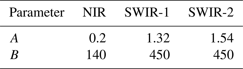
In order to be as consistent as possible with real measurements, random noise has been added to the simulated spectra. This noise N has been calculated for each radiance R using band-specific parameters A and B via
The assumed values for A and B are given in Table 2. These values were derived from a study on CO2M requirements and performance (Buchwitz et al., 2020) and have been shown to be consistent with the measurements of the selected CO2M detectors.
Table 2Parameters of instrument noise model. Unit of A is 10−7 (photons s−1 nm−1 cm−2 sr−1)−1.
2.1 Full-year global subset
To assess the impact of large-scale temporal and spatial variations on the FOCAL-CO2M results, a global data set covering at least a full year is required. However, SCIATRAN simulations are computationally expensive. Therefore, it is not currently feasible to compute a complete CO2I full-year data set for one of the CO2M satellites within a reasonable time. For the full-year data we therefore selected a subset of CO2I measurement geometries containing every 15th out of 110 across-track ground pixels and every 20th out of roughly 9200 along-track scan lines per orbit for solar zenith angles lower than 80°. This results in a subset with 300 times less data than the whole CO2M data set, but with similar spatial and temporal coverage. The meteorological information (pressure, temperature, water vapour) used in the SCIATRAN simulations is taken from the fifth generation of the ECMWF reanalysis (ERA5) data (Hersbach et al., 2020) (temporal resolution 1 h, spatial resolution 0.25°). CO2 and CH4 profiles use the results from the CAMS model data for 2015 (spatial resolution about 2° × 3°), namely v20r1 for CO2 (Chevallier et al., 2005, 2010; Chevallier, 2013) and v20r1 for CH4 (Segers, 2022). The reflectivity of the surface is modelled using BRDF parameters from the Moderate Resolution Imaging Spectroradiometer (MODIS) MCD43C1 Version 6.1 BRDF and albedo model parameters data set (Schaaf and Wang, 2021). These BRDF parameters have been interpolated spectrally to the centres of the three CO2I bands. Within one band, the BRDF is assumed to be constant for the SCIATRAN calculations. We also tested a linear wavelength dependency of the BRDF within the bands, but this only resulted in a change of the derived polynomial parameters for the surface albedo which – in combination with an adapted post-processing – did not significantly change the derived XCO2 and XCH4 results. Solar-induced chlorophyll fluorescence irradiance is simulated by scaling an irradiance spectrum obtained from the publication of Rascher et al. (2009). The scaling factor is obtained by assuming a linear relationship between SIF irradiance at 740 nm and MODIS NDVI (Didan, 2021) derived by the Rutherford Appleton Laboratory (RAL, 2022). Clouds in the data set are considered by SCIATRAN using ERA5 specific cloud liquid water content and specific cloud ice water content as input. However, for the current study we only consider completely cloud-free soundings. Aerosol is simulated in SCIATRAN using as input different aerosol types, phase functions, single scattering albedo and vertical distribution of the mass mixing ratio, considering dependencies of particle size on humidity. These aerosol parameters are taken from the CAMS global reanalysis EAC4 (Inness et al., 2019). Land–water information is taken from GTOPO30 (Earth Resources Observation and Science Center, U.S. Geological Survey, U.S. Department of the Interior, 1997), and surface altitude–pressure is taken from ERA5. The SCIATRAN calculations have been performed in scalar mode without consideration of inelastic scattering processes. This is expected to have only a minor impact on the retrieval results, which has been tested using simulated data from the RAL (2022) study as input. SCIATRAN (and also FOCAL) is run in plan-parallel mode, although both SCIATRAN and FOCAL could consider sphericity; however, in the case of CO2M (normally nadir looking with a swath of about 240 km, relevant solar zenith angles less than 75°), spherical geometry has no major impact and is therefore neglected. We also assumed a uniform scene within each ground pixel. So far, only nadir data over land are modelled, which results in a total of about 6 million spectra per year for each band.
Although the SCIATRAN calculations are quite complex compared to the more simple FOCAL forward model, they do not consider all possible physical processes like 2D/3D effects of clouds and aerosols. However, even if the radiative transfer model would be able to consider this, the required input data are usually not available. This is a general limitation of all forward models.
Figure 1 shows an example for the sampling of the XCO2 subset data over part of Europe for one CO2M orbit (only data over land). The shown region corresponds to the range of the high-resolution scene addressed in the following sub-section.
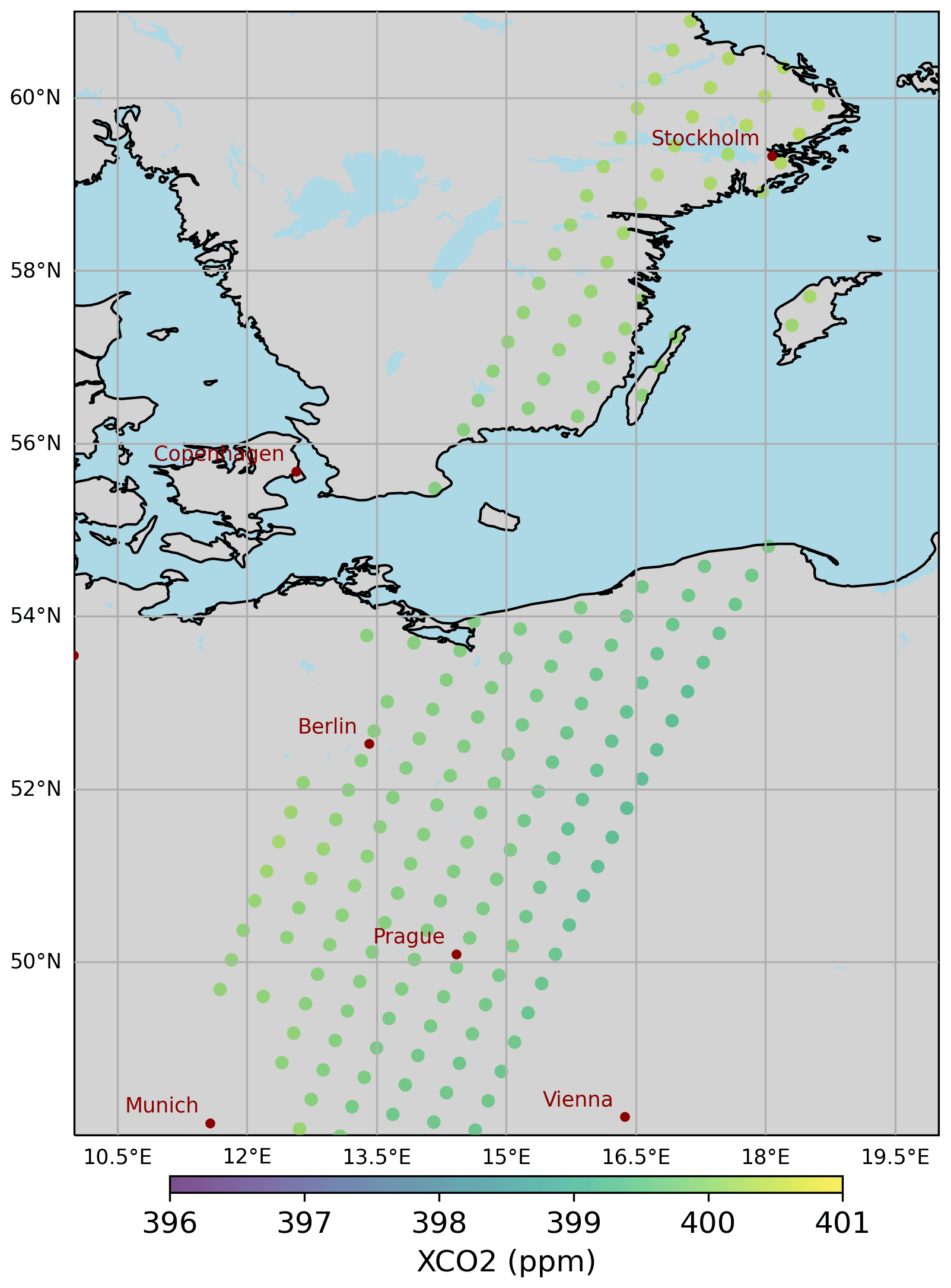
Figure 1Example for the subset data: modelled XCO2 over part of Europe for one orbit on 3 July 2015. Only cloud-free data over land are shown because only these will be used later in the retrieval. No post-processing filters are applied. Note that only the centre points of the ground pixels are plotted and that the size of the markers is much larger than the original ground pixel size.
2.2 High-resolution scene
In addition to the full-year global subset data, we used SCIATRAN to model also the NIR and SWIR radiances for a full 3 min granule of CO2I data containing about 67 000 measurements, of which about 37 000 are over land and cloud-free. This granule from 3 July 2015 (referred to as the “Berlin scene”; see Fig. 2) is one of the typical test scenes, used within the CO2M project, because of the availability of high-resolution model data for this scene. The calculations for the high-resolution scene use the same SCIATRAN setup except for geolocation, geopotential, pressure, temperature, specific humidity, CO2 and CH4, which were provided by EUMETSAT using high-spatial resolution (9 km) data from the CAMS nature run model (Agustí-Panareda et al., 2022). As can be seen from Fig. 2, with this resolution XCO2 plumes from power plants in eastern Germany are clearly visible, although the increase of XCO2 in these plumes is only a few parts per million (ppm) above background. Figure 3 shows the corresponding XCH4 data.

Figure 2High-resolution scene: XCO2. Only cloud-free data over land; no post-processing filters are applied.
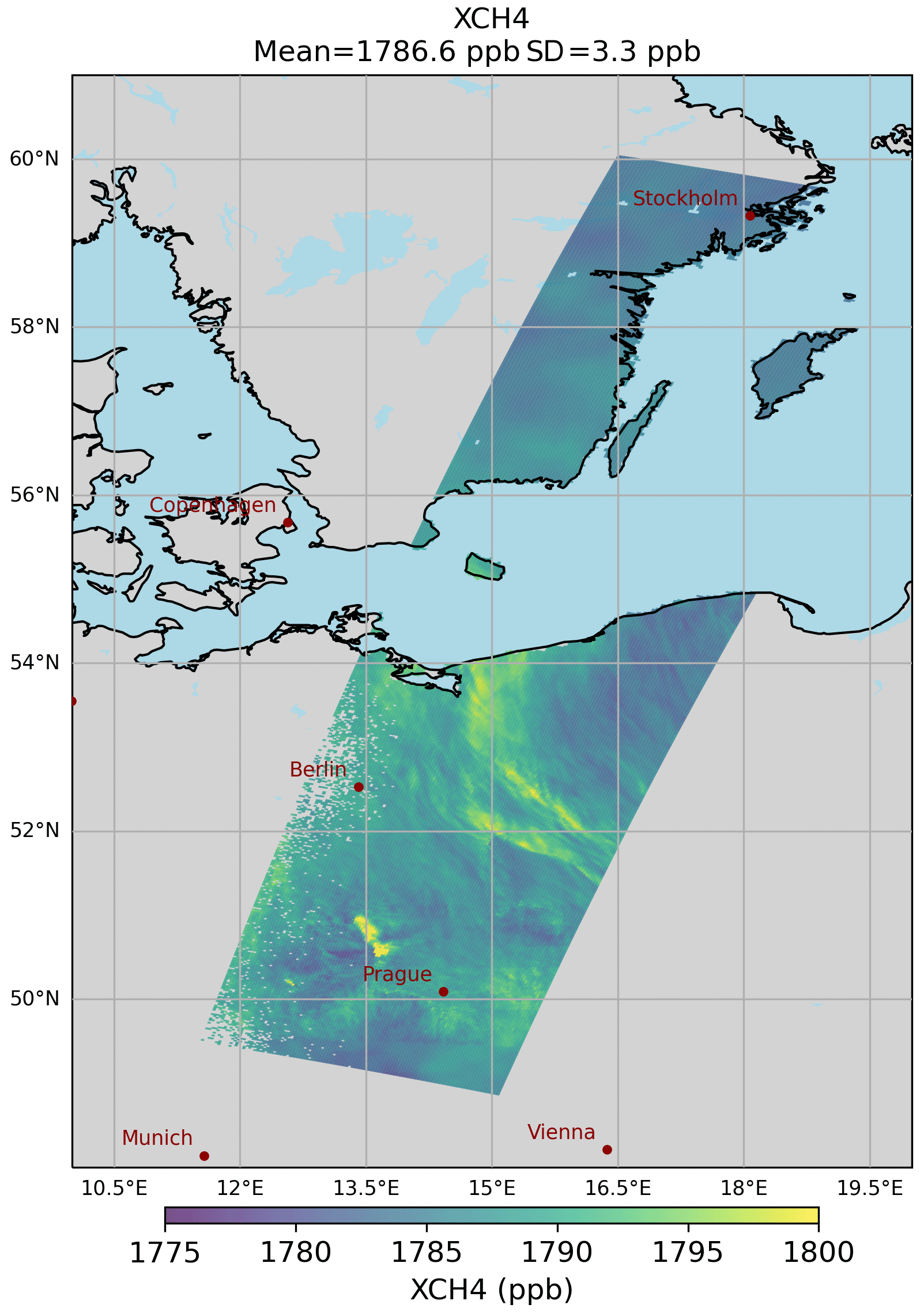
Figure 3As Fig. 2 but for XCH4.
3.1 FOCAL-CO2M retrieval
The FOCAL retrieval method is based on optimal estimation. FOCAL models the propagation of light through the atmosphere. Scattering is approximated by an infinitely thin single scattering layer, which is characterised by the vertical position of the layer (pressure relative to surface pressure), the optical thickness of the layer and the Ångström exponent describing the wavelength dependence of the scattering (see e.g. Reuter et al., 2017b, for details). Scattering at this layer is assumed to be isotropic. All scattering quantities are effective; they describe the whole scattering (including, for example, Rayleigh scattering) and thus should not be interpreted as, for example, aerosol properties. The FOCAL forward model divides the atmosphere into 20 layers, which are defined such that they contain the same number of dry-air molecules. Inside a layer, all atmospheric parameters are assumed to be constant. In the retrieval, FOCAL determines the concentrations (sub-columns) for five output layers, each also containing the same number of molecules. The layers are fitted individually such that the shape of the profiles may change. However, the amount of change is limited by the use of an a priori covariance matrix. In the present case, we use for XCO2 and XCH4 matrices derived from the Simple cLImatological Model (SLIM; see Noël et al., 2022), which give a reasonable variability. The final XCO2 and XCH4 is then derived from the average of the corresponding sub-columns in each layer.
Applications to OCO-2, GOSAT and GOSAT-2 have shown that FOCAL is fast and produces accurate results. For example, the spatio-temporal bias of the FOCAL XCO2 product derived from TCCON comparisons is (after bias correction) in the order of 0.6 ppm for OCO-2 (Reuter and Hilker, 2022) and 0.6 (1.1) ppm for GOSAT (GOSAT-2) (Noël et al., 2022). FOCAL is therefore well suited for the analysis of large data sets.
FOCAL-CO2M is an adaptation of the FOCAL method for use in the CO2M mission. FOCAL permits full physics (FP) and proxy (PR) retrievals. FP retrievals are based on directly retrieving the quantity of interest, i.e. XCO2 or XCH4, whereas PR retrievals are based on computing the ratio of the retrievals of the two gases and using modelled XCO2 or XCH4 for correction (see e.g. Schepers et al., 2012, for details). The main output products of the FOCAL-CO2M retrieval are total column FP XCO2 and XCH4, but there will also be corresponding additional PR data and SIF and water vapour (XH2O) products. However, in the current study we only consider the FP XCO2 and XCH4 products.
The retrieval consists of three steps: pre-processing, inversion and post-processing.
The inputs to the pre-processing include (1) the spectral data from CO2I (measured radiances and their uncertainties as well as related measurement times and measurement geometry, geolocation, etc.) and (2) related meteorological information and a priori profiles for the considered gases. For the current study, we use simulated data; see Sect. 2.
The objective of pre-processing is to filter the input data to minimise the waste of computational time for unsuitable atmosphere and ground scenes or soundings. For the purpose of this study, we filter out all cloudy data and data over water surfaces, because these are not required for the verification of the systematic error requirements. However, the retrieval is also planned to be applied to data over ocean, especially in glint mode. We also remove all data with solar zenith angles larger than 75° and data for which the signal-to-noise ratio is lower than 100 at the wavelengths, 755, 1624 and 2036 nm, i.e. one spectral region in each band where absorption is low.
The inversion uses an optimal estimation retrieval approach (Rodgers, 2000). It has four fitting windows in the near-infrared (NIR) and short-wave-infrared (SWIR) spectral regions; see Table 3. The corresponding state vector elements and their a priori values are listed in Table 4. The assumed a priori uncertainties for the gas profiles consider covariances and are the same as those used in GOSAT and GOSAT-2 FOCAL retrievals, which were derived based on the SLIM (Simple cLImatological Model for atmospheric CO2 or CH4) climatology (see Noël et al., 2022, for details). As for OCO-2, GOSAT and GOSAT-2, we consider an additional forward model error in the retrieval, which takes into account possible limitations of the forward model and is determined from the simulated CO2M measurements; see e.g. Reuter et al. (2017a, b) for details. The instrument line shape (ILS) functions are currently assumed to be Gaussian with a full width at half maximum (FWHM) as given by the spectral resolution in Table 1.
Table 3Definition of FOCAL-CO2M spectral fit windows. Cross sections are from HITRAN2016 (Gordon et al., 2017, downloaded on 23 March 2021).
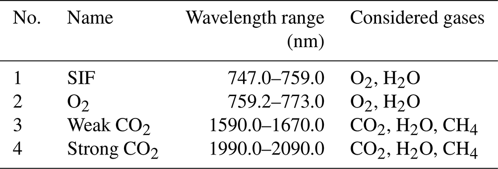
Table 4State vector elements and related retrieval settings. A priori values are also used as first guess. “Fit windows” lists the spectral windows (see Table 3) from which the element is determined; “each” means that a corresponding element is fitted in each fit window. A priori values labelled as “PP” are taken from the provided meteorological data; “est.” denotes that they have been estimated from the background signal.

During post-processing, the output data from the inversion are filtered for outliers. Furthermore, a bias correction is performed to remove systematic offsets arising, for example, from limitations of the forward model. The underlying database for the post-processing is generated using a subset of (uncorrected) retrieval results as input. Here, we use the results of the retrieval after inversion for the April 2015 subset data. We only use 1 month of data instead of the whole year for the following reasons:
-
we want to be as close to real conditions as possible – during the commissioning phase we need to re-determine the post-processing database, and there will be most likely only a limited amount of data available at that time;
-
with the current setup it is possible to show that the post-processing is working also for data and/or time periods which were not used during generation of the database.
The retrieval results for April 2015 are then filtered for convergence and fit quality. Using these data, the current post-processing database has been derived as follows.
The filtering of the data is similar to the filtering performed for OCO-2 and GOSAT(-2) data and comprises two filtering steps (see e.g. Noël et al., 2022, for details). First, data are filtered for retrieval quality (see Reuter et al., 2017b). Second, additional filter parameters and their limits are determined using a variance minimisation method. The idea of this second step is that outliers largely contribute to the scatter, and the method finds thresholds for parameters which most efficiently remove these outliers from the final data set.
Within this second step, an iterative procedure is used to determine a set of a maximum of 10 parameters which have the largest effect on the variance reduction of the bias, i.e. the difference between the retrieved value and an assumed “true” value, for a prescribed percentage of data to be filtered out. The percentage of data to be filtered out is a trade-off between the remaining scatter of the data and the number of remaining data after filtering. For the simulated data used in the present study we prescribed that 15 % shall be removed.
The bias correction is based on a machine learning regression, which determines the function and the 10 (or less) best parameters to reduce the bias based on a set of training and test data (each 50 % of the input data). This is similar to the method described in Noël et al. (2022), but here we use a regression based on a gradient-boosting method (currently XGBoost, Chen and Guestrin, 2016) instead of a random forest regression. For the current test data set, XGBoost performs better than random forest regression.
The final determination of the post-processing databases is done in an iterative way:
-
apply the first-step basic filtering for retrieval quality;
-
determine and apply the bias correction to the resulting basically filtered data set;
-
determine the (final) filter settings using the variance filter method with the data from the previous step as input;
-
apply these filters to the basically filtered data from step 1;
-
determine the (final) bias correction based on the output data from the previous step.
Performing a preliminary bias correction before the determination of the filter settings has the advantage that data which can be sufficiently well corrected via the bias correction are not necessarily filtered out.
For simulated data, the true XCO2 and XCH4 values are perfectly known, because they have been used for the generation of the simulated spectra. Therefore, the current filtering and bias correction does not consider any additional errors resulting in systematic differences between the estimated meteorological conditions and the actual atmosphere. The impact of this additional error source on the retrieval results can only quantified by comparisons of real measurements with independent data. The retrieval results presented later therefore do not include the impact of limited knowledge of the true values.
Tables 5 and 6 show the derived filter parameters and their limits for XCO2 and XCH4, respectively. As can be seen from these tables, only filters on polynomial parameters and their errors were applied, although the derived scattering parameters were also possible candidates. This means the filtering of the simulated data is based on surface albedo properties.
Table 5Filter variables and limits for FOCAL-CO2M XCO2 (land). “–” means that no limit is applied.
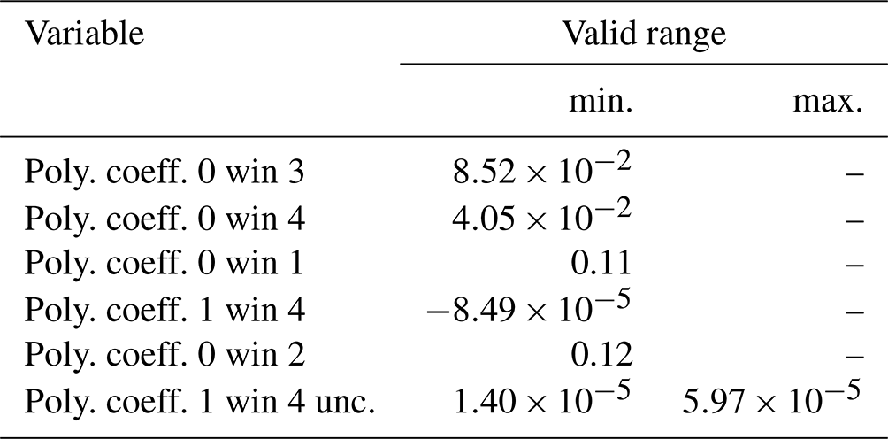
Table 6Filter variables and limits for FOCAL-CO2M XCH4 (land). “–” means that no limit is applied.
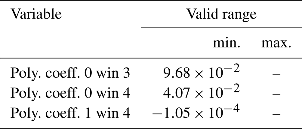
Figure 4 shows the derived bias correction parameters as a function of their importance. For both XCO2 and XCH4 the most relevant parameter for the bias correction is the derived Ångström coefficient. This means that largest (uncorrected) biases are related to scattering, i.e. most likely aerosol since we are using only cloud-free data here. This also indicates that there is a strong correlation between the derived scattering parameters and aerosol abundance.
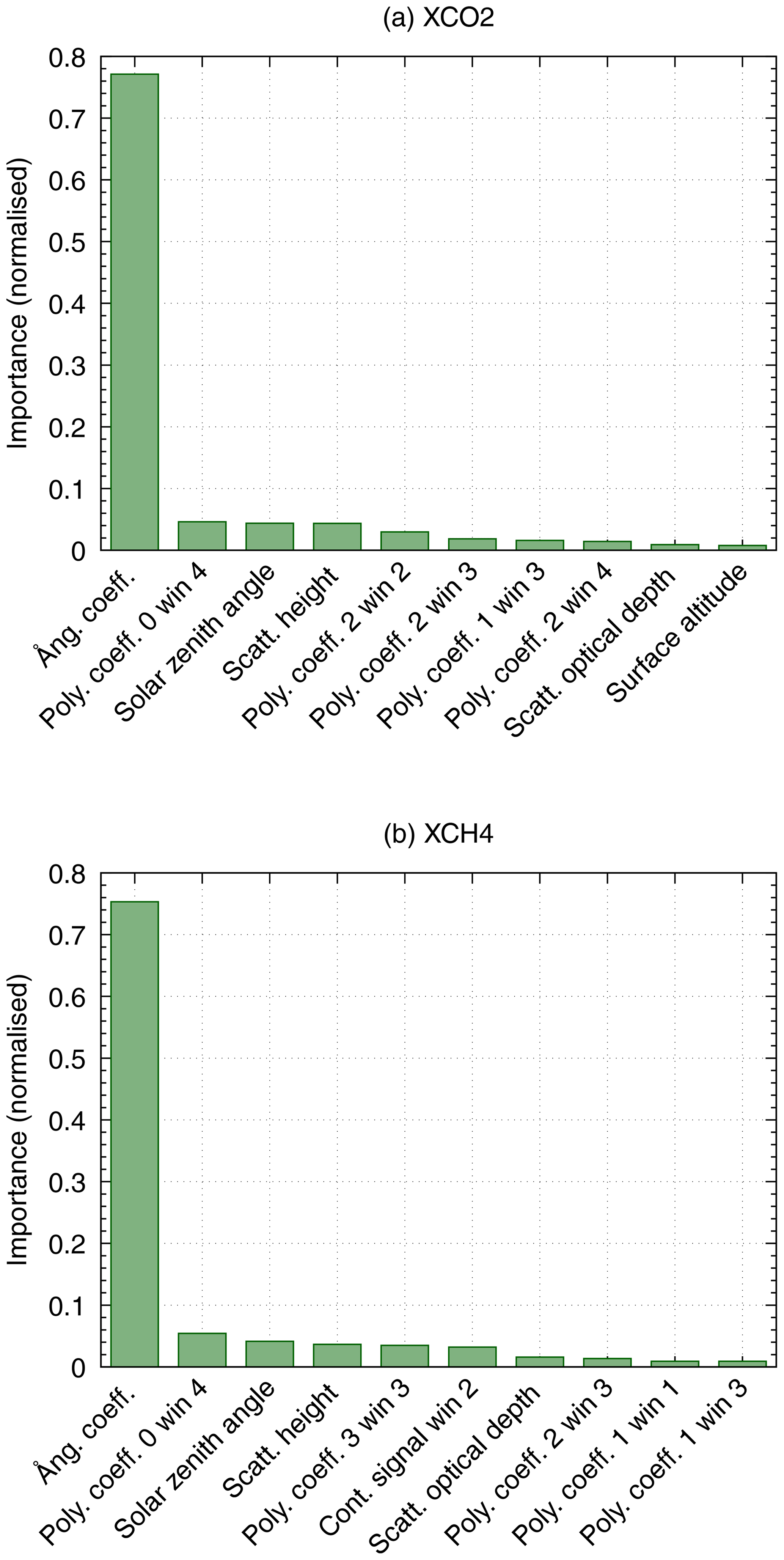
Figure 4Bias correction parameters and their relative importance (normalised such that the sum of all importances is 1). (a) XCO2. (b) XCH4.
As an example for the spatial distribution and magnitude of the bias correction, Figs. 5 and 6 show the derived values for XCO2 and XCH4. The mean correction is small (0.1 ppm for XCO2 and 2.1 ppb for XCH4), but there are significant local differences. Larger corrections occur over northern Africa, the Arabian Peninsula and India, i.e. regions with typically larger surface albedo and aerosol load.
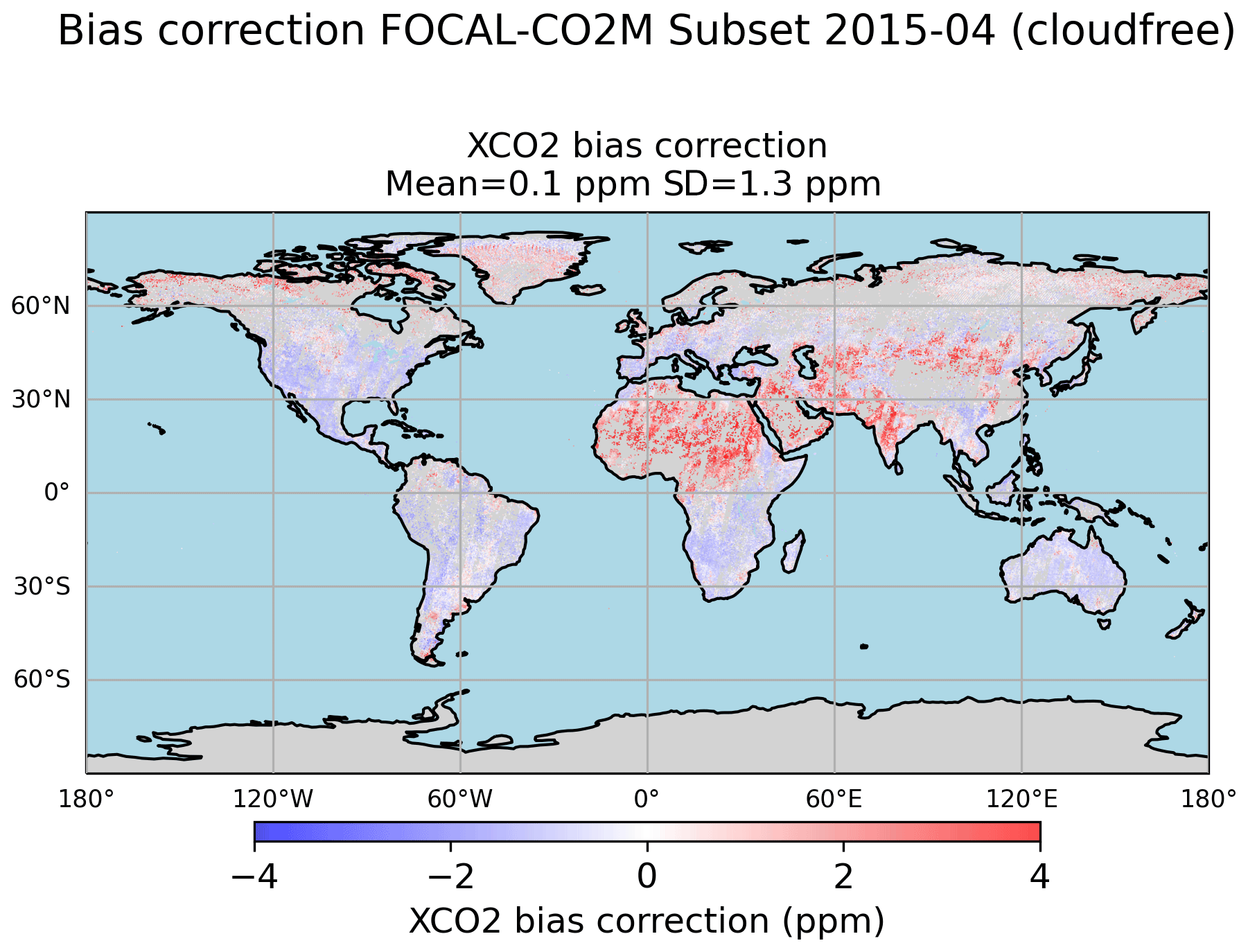
Figure 5Map of the derived XCO2 bias for the subset data of April 2015.
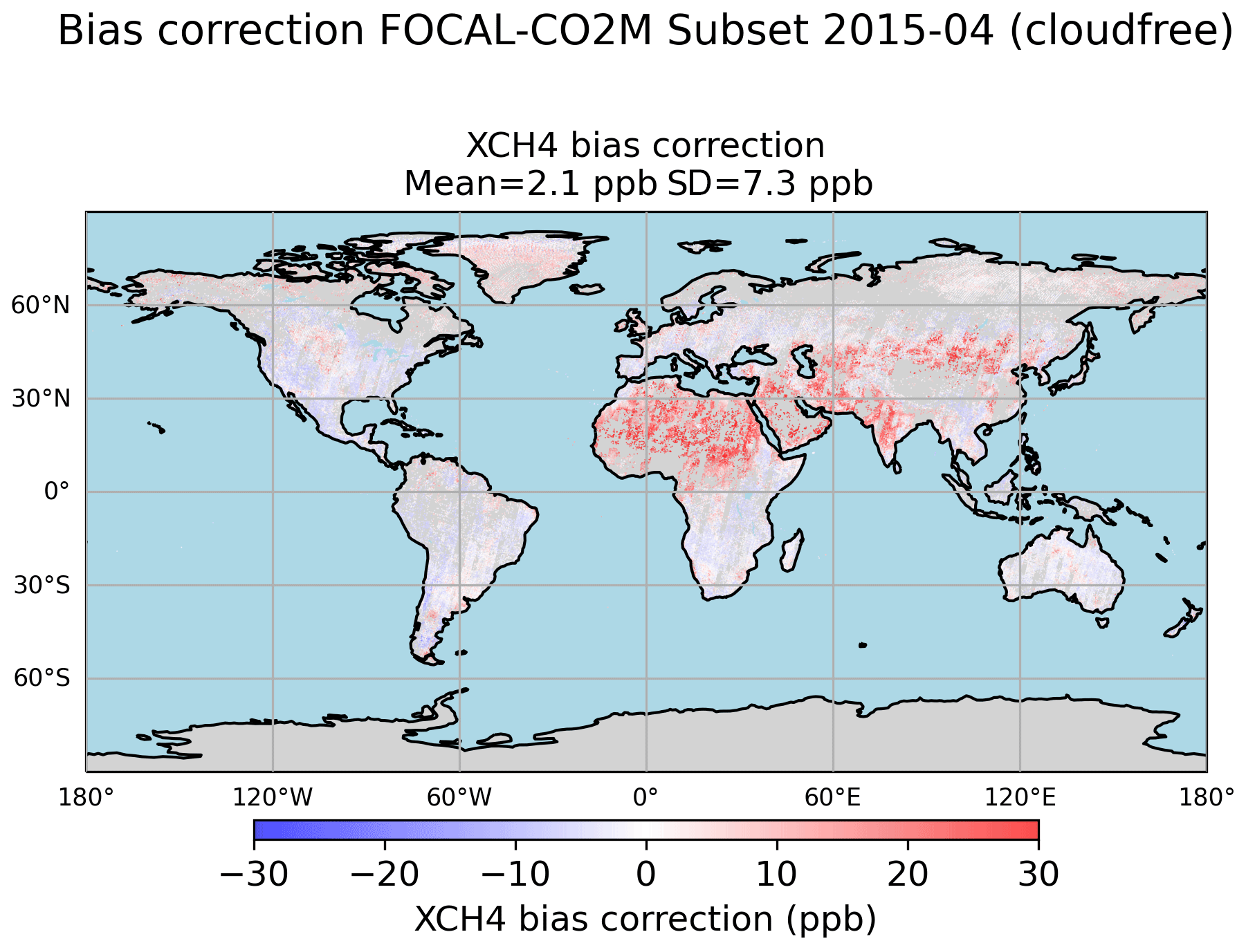
Figure 6As Fig. 5 but for XCH4.
Note that the quality of the post-processing may in principle be improved by extending the input data set used to determine the post-processing database (especially regarding the training of the bias correction). However, at the beginning of the CO2M mission, the amount of available measurement data will be limited. In order to show that our post-processing would even work with a minimum amount of data, we use only 1 month of simulated data here.
3.2 Adaptations for real data
The FOCAL-CO2M retrieval software has been designed such that it can be applied to both simulated data (as in the present study) and to real measurement data. However, the application to actual measurements requires some adaptations.
This includes the incorporation of results from the on-ground calibration (e.g. updated ILS data) as well as updates of filtering and bias correction parameters, which can only be determined during the commissioning phase based on the analysis of in-flight measurements.
In the pre-processing, cloud and signal-to-noise filters need to be adjusted. For the retrieval, the forward model error needs to be re-determined. Furthermore, the post-processing database needs to be re-calculated using adapted filter settings and bias correction parameters. It also has to be checked if additional information, for example, aerosol parameters derived by the MAP instrument, may be used in both pre- and post-processing.
3.3 Performance assessments
The primary objective of this study is to obtain a first estimate of the performance of the FOCAL-CO2M retrieval with respect to known sources of systematic errors. As already mentioned above, the corresponding requirements for the resulting XCO2 and XCH4 are high (systematic error ≤ 0.5 ppm and 5 ppb, respectively); see ESA (2020).
However, these requirements are formulated in a general way. Therefore, there is a need for some interpretation to verify these requirements. We consider that the requirements should be verified by using cloud-free data over land only. Furthermore, the interpretation of systematic errors depends on the application, i.e. the purpose for which the data shall be used. CO2M has two main application areas:
-
quantification of anthropogenic emissions;
-
quantification of natural large-scale fluxes.
For the quantification of anthropogenic emissions it is important that local enhancements (e.g. emission plumes) can be separated from the background. The background values themselves are less important. A verification therefore requires spatially highly resolved scene data with, for example, emission plumes.
For the quantification of natural large-scale fluxes, local variations are less relevant. Here, it is important that large-scale structures and their variations in both time and space are correct. This requires global data covering at least a full year to consider possible long-term and/or large-scale errors.
According to the ESA (2020), CO2 plume imaging (i.e. anthropogenic emissions) is the driving application for the precision requirements. Nevertheless, knowledge about larger-scale or areal fluxes is also important for global modelling. Therefore, we consider both applications here. The verification of the requirements thus has to take these different scales into account. In the following sub-section we describe the verification methods for both application areas.
For the verification of the systematic error requirements for natural large-scale fluxes, we use the retrieval results from the full-year global subset measurements as these provide a good spatial and temporal coverage. We then determine a running average of the difference between the retrieved value and the true value within a 1° × 1° latitude–longitude box. This results in a low-pass-filtered bias data set. For this data set we compute the standard deviation, considering the cosine of the latitude as weights to account for different sizes of the averaging area. To fulfil the systematic error requirement, the resulting weighted standard deviation of the low-pass-filtered bias should then be ≤ 0.5 ppm.
For the verification of the systematic error requirements for anthropogenic emissions, we take as input the high-resolution Berlin scene. We then apply – as for the large-scale fluxes – a 1° × 1° low-pass filter to the difference between the retrieved value and the true value, which results in a spatially smoothed bias. This smoothed bias is then subtracted from the original data, which gives us a high-pass-filtered bias data set (for this scene). The standard deviation of these high-pass-filtered bias data should then be ≤ 0.5 ppm to fulfil the requirement for systematic errors.
Figure 7 shows as an example for the different filtering procedures the unfiltered XCO2 bias (retrieved minus true values) for the high-resolution Berlin scene and the resulting low- and high-pass-filtered bias.

Figure 7Example for low- and high-pass filtering (Berlin scene). (a) Bias (FOCAL-CO2M retrieved minus true XCO2). (b) 1° × 1° low-pass-filtered bias. (c) The high-pass-filtered bias is the bias minus the low-pass-filtered bias.
4.1 Application to anthropogenic emissions
As explained above, the verification of the performance requirements for anthropogenic emissions is achieved by using the high-resolution Berlin scene.
Figure 8 shows the FOCAL-CO2M XCO2 retrieval results for this scene. The retrieved XCO2 (after post-processing) is shown in the left plot, the true XCO2 in the centre and their difference in the right plot. Some statistical information is also given in the figure below these plots. Note that these are rounded values.
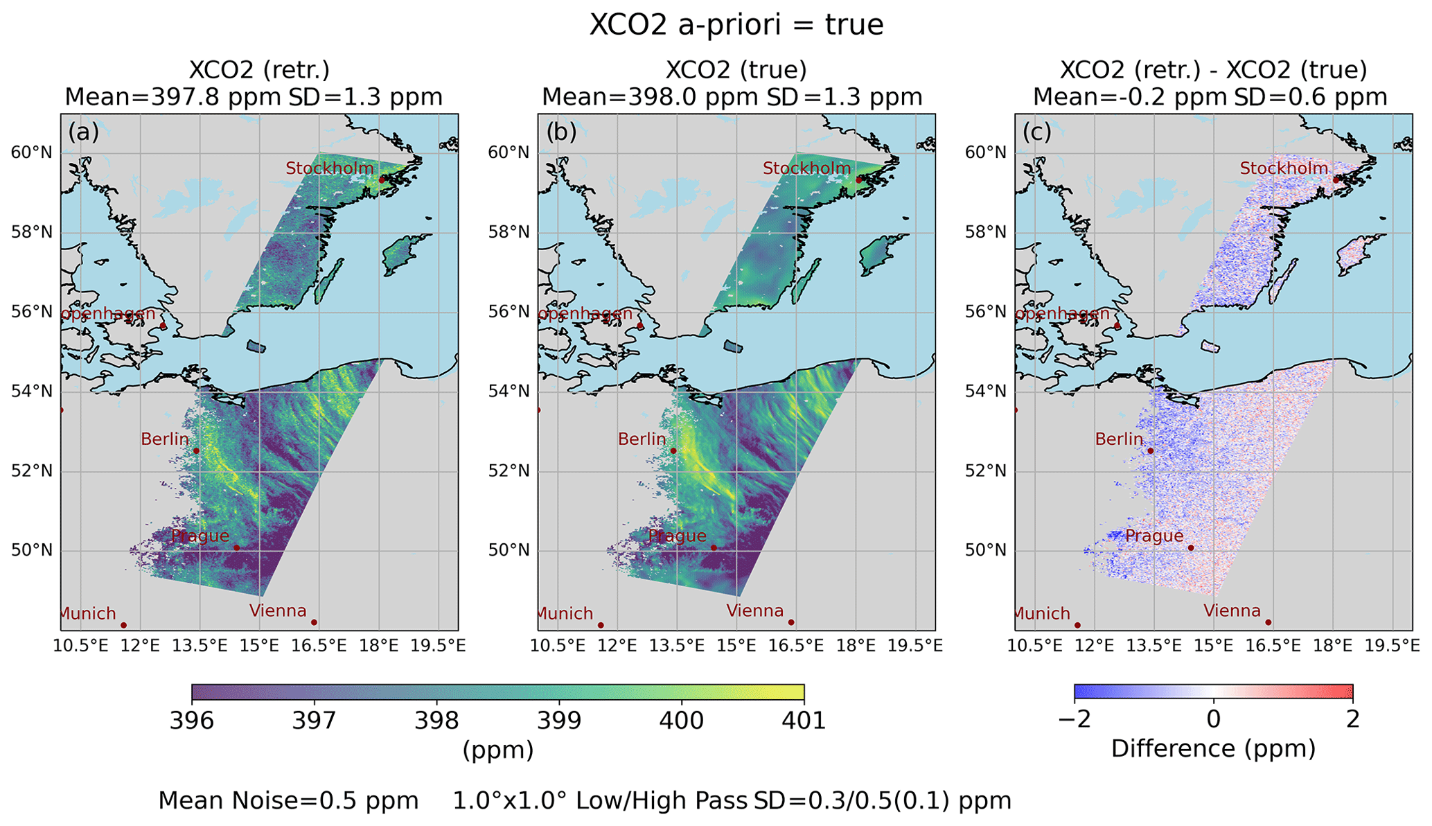
Figure 8FOCAL-CO2M XCO2 retrieval results for the Berlin scene (only cloud-free data over land). (a) Retrieved XCO2. (b) True XCO2. (c) Difference retrieved minus true XCO2. The same post-processing filtering has been applied to all data shown in the plots. The number in brackets after the high-pass standard deviation gives an estimate for the high-pass standard deviation without noise.
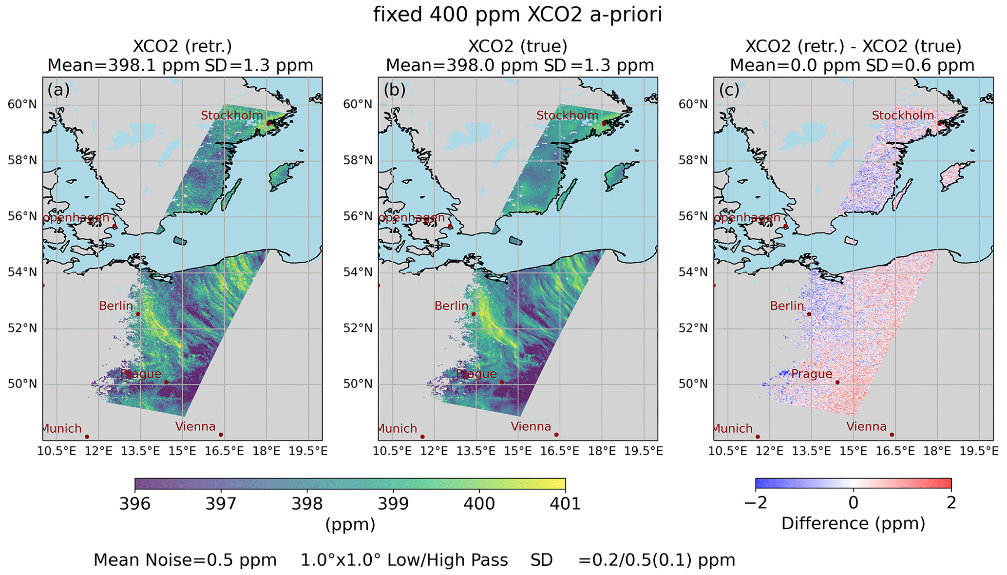
Figure 9As Fig. 8 but for a fixed 400 ppm a priori CO2 profile.
All structures of the scene shown in the true XCO2 can also be identified in the retrieved data. The mean difference between the retrieved and the true XCO2 is −0.2 ppm. The standard deviation of the difference is 0.6 ppm. After application of the low- and high-pass filters this reduces to 0.2 and 0.5 ppm. The values for the high-pass-filtered data do not only contain the systematic error component but also the noise on the data. The (rounded) mean noise error of the data in this scene is also about 0.5 ppm. This means that the high-pass standard deviation is dominated by noise; thus, the real systematic error is probably well below 0.5 ppm. If we subtract the noise-related variance from the high-pass variance and then take the square root, we get the value given in brackets after the high-pass variance in the plot, namely 0.1 ppm. This can be considered as a lower estimate for the high-pass standard deviation as it does not consider potential systematic error contributions to the a posteriori noise error.
The average a posteriori error of the retrieved XCO2 (including the noise and the smoothing error) is about 0.6 ppm, i.e. very close to the noise error. Compared to the assumed a priori uncertainty for CO2 of 5 ppm (see Table 4) this corresponds to an uncertainty reduction of about a factor of 8.
A small gradient is visible in the difference between the retrieved and the true XCO2 from north-east to south-west. This could be related to aerosol effects. In this scene, most aerosol is located in the south-west. Differences in the handling of surface properties by SCIATRAN and FOCAL could also play a role. However, since we are interested in the quantification for anthropogenic emissions, these larger-scale effects are less relevant.
As mentioned in Table 4, the XCO2 a priori values used in the retrieval are taken from the meteorological data, which where also used in the generation of the input spectra. They are therefore identical with the true values. This is because we aim to be as consistent as possible with the procedures to be applied to real data at a later time, and for real measurements we will also use the (predicted) meteorological input data as truth for the post-processing corrections. However, in reality of course the truth will deviate from the model data. To show that the sensitivity of the retrieval to the choice of the a priori CO2 profile is low, we have performed the retrieval for the Berlin scene also for a fixed CO2 a priori profile for all measurements by assuming a constant value of 400 ppm for all altitudes. As can be seen from Fig. 9, this has hardly any impact on the retrieval results. All XCO2 features can be reproduced even with the fixed a priori profile. There is only a small mean offset of about 0.2 ppm compared to the values where the true XCO2 was used as a priori.
Figure 10 shows a zoom-in of Fig. 8 on the region of the power plants in eastern Germany. Despite the noise on the data, the plumes from the different power plants can be clearly identified in the retrieval results. No plume structures are visible in the difference map. The high-pass standard deviation for this sub-scene is 0.5 ppm, similar to the noise error. The high-pass standard deviation is thus also dominated by noise. Subtraction of the noise contribution results in a standard deviation of 0.1 ppm. The requirement for systematic errors is therefore fulfilled for XCO2 for this scene. Note that in reality 2D/3D effects (vertical and/or horizontal distribution of the plume), which are not fully considered in our simulations, may affect the results. This can only be checked with real data.
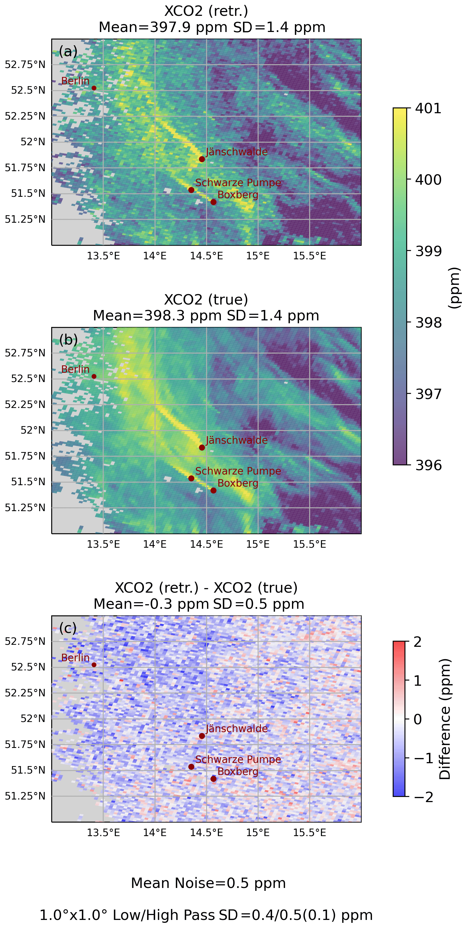
Figure 10Zoom of Fig. 8.
The results for XCH4 using the true values as a priori are shown in Fig. 11. For this case, also the main structures of the true XCH4 field are re-produced in the retrieval. As for XCO2, the difference between retrieved and true XCH4 is dominated by noise. The mean offset for this scene is −1.4 ppb, with a standard deviation of the (unfiltered) difference of 5.2 ppb, including a noise error of 4.8 ppb. The average a posteriori error for XCH4 is 5.8 ppb, compared the a priori uncertainty for CH4 of 45 ppb from Table 4. The uncertainty is therefore reduced as for CO2 by about a factor of 8.
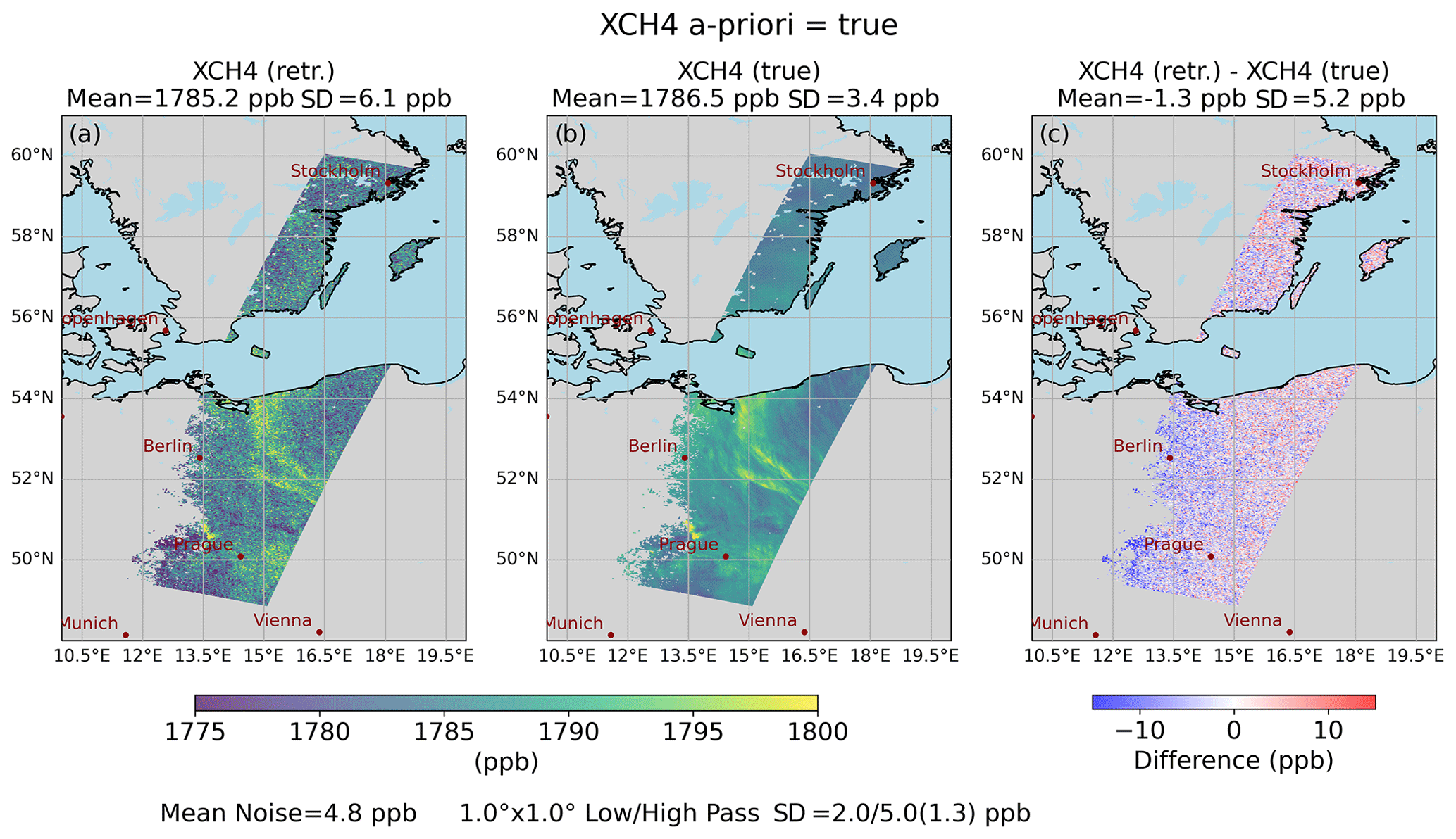
Figure 11As Fig. 8 but for FOCAL-CO2M XCH4.
The high-pass-filtered mean standard deviation is 5.0 ppb with a lower (noise-corrected) estimate of 1.3 ppb. The requirement of a maximum of 5 ppb is therefore fulfilled. The difference map for XCH4 shows a similar gradient as for XCO2 from north-east to south-west, most likely for the same reasons.
4.2 Application to large-scale fluxes
The verification of the requirement for large-scale natural fluxes is based on the full-year global subset data. As an example, Fig. 12 shows the FOCAL-CO2M XCO2 retrieval results for April 2015. The corresponding XCH4 data are shown in Fig. 13.

Figure 12FOCAL-CO2M XCO2 retrieval results for April 2015 (cloud-free subset data over land). (a) Retrieved XCO2. (b) True XCO2. (c) Difference retrieved minus true XCO2.

Figure 13As Fig. 12 but for XCH4.
As can be seen from these figures, the retrieved data reproduce all large-scale patterns present in the true/a priori data. The scatter in the differences between retrieved and true values is dominated by noise. Since the April 2015 data are used in the derivation of the post-processing databases, Figs. 12 and 13 show the best case. However, the quantitative assessments described in the following show that other months have a similar performance.
For these quantitative assessments of the systematic error for large-scale fluxes, we apply a low-pass filter to the differences and determine the weighted standard deviation for the low-pass-filtered data as described in Sect. 3.3. This is done for each month as well as for the whole year 2015. The results are shown in Figs. 14 and 15.

Figure 14Monthly means and standard deviations of 2015 global subset data. (a) Mean difference retrieved minus true XCO2. (b) Standard deviation retrieved minus true XCO2 (orange: unfiltered; red: low-pass-filtered). (c) Number of data after post-processing. Annual values are given in the labels.
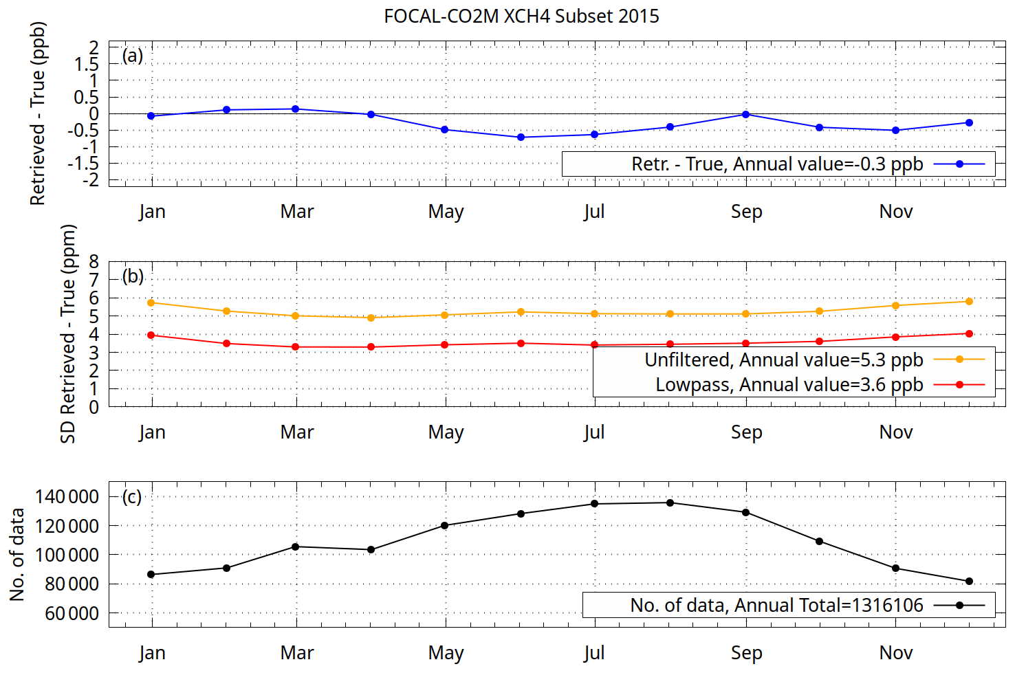
For the verification of the systematic error requirements the red line in the middle plots is relevant. It shows the weighted standard deviation for the low-pass-filtered data for each month and the value for the complete year (i.e. not the average over the monthly data) in the legend of each panel.
The yearly average low-pass standard deviation for XCO2 is 0.5 ppm and therefore just fulfils the systematic error requirement for large-scale fluxes. For XCH4, the yearly average low-pass standard deviation is 3.7 ppb and therefore smaller than the required 5 ppb.
The lowest XCO2 and XCH4 standard deviations are achieved in April 2015. The biases at this month are also zero. This is not surprising, because this is the month which was used for the training of the bias correction. Slightly higher standard deviations occur in other months, but the standard deviations of the low-pass-filtered data are always below 0.6 ppm for XCO2 and 4 ppb for XCH4. The largest standard deviations occur for both gases in December and January, where also the number of valid data is lowest. In general, it is expected that the results improve if more months (e.g. a full-year subset data set) are used for the generation of the post-processing database.
However, the simulated data used here do not fully represent reality because of the limitations and underlying assumptions in the radiative transfer and the retrieval. Even under these conditions the estimated systematic errors for large-scale fluxes are especially for XCO2 very close to the requirements. This indicates that fulfilling these requirements for real data might be possible but will be a challenge.
4.3 Aerosol dependence
Up to the present, the FOCAL-CO2M retrieval does not use any external information about aerosols (e.g. from the MAP instrument). The systematic error requirements are only applicable up to an aerosol optical depth of 0.5 (ESA, 2020). Therefore, we also checked the aerosol dependence of the FOCAL-CO2M retrieval results. Figures 16 and 17 show the (binned) differences between the retrieved and the true XCO2 and XCH4 for the full-year 2015 subset data as a function of the aerosol optical depth (AOD) at 550 nm, which was assumed for the generation of the simulated spectra with SCIATRAN.
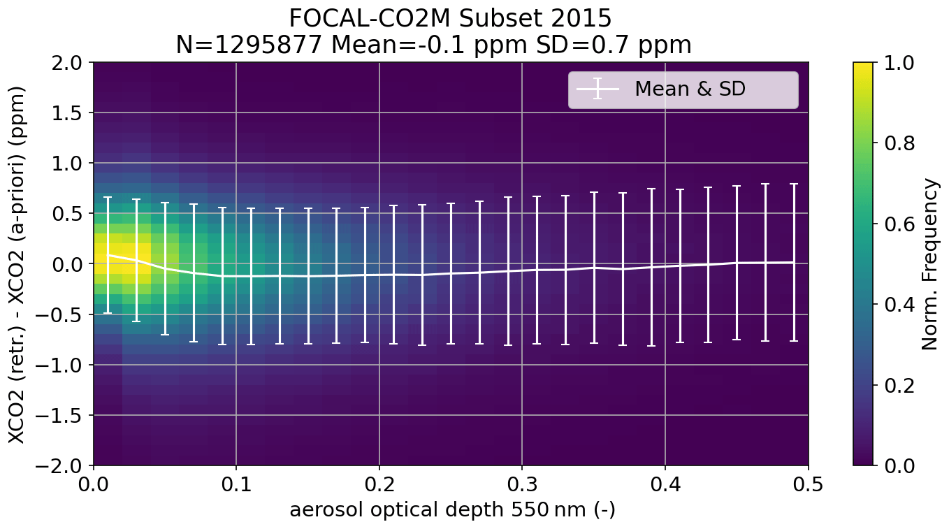
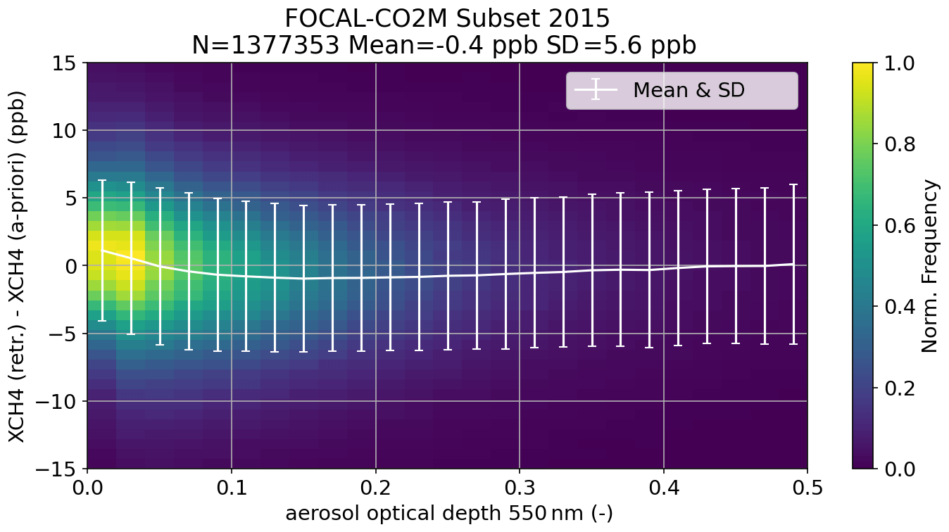
As mentioned above, the SCIATRAN calculations for the simulated data consider different aerosol types and distributions, but the FOCAL retrieval does not explicitly consider aerosol – it assumes only one effective scattering layer. Nevertheless, as can be seen from Fig. 16, mean systematic offsets due to aerosol for the complete year are less than about 0.2 ppm for XCO2 with a mean of zero for all AODs up to 0.5. The standard deviation of the XCO2 difference is on average 0.7 ppm and typically smaller for lower AOD. The functional dependence on AOD is similar for XCH4 (see Fig. 17). Systematic XCH4 offsets are usually smaller than 1 ppb.
These results could possibly be improved when using extended training data for the post-processing and/or additional information from the MAP instrument.
FOCAL is one of three retrieval algorithms under development for the operational retrieval of XCO2, XCH4 and other parameters from the constellation of CO2M satellites to be launched from 2026 onward. These data products contain information on anthropogenic and natural sources and sinks of the two greenhouse gases CO2 and CH4, which will be extracted using appropriate inverse modelling to support emission monitoring in the context of the Paris Agreement on climate change. This application requires high accuracy as even small biases can lead to significant emission errors (ESA, 2020).
The FOCAL retrieval has been successfully adapted to simulated CO2M data. First performance tests using data simulated with SCIATRAN as input have been performed. Based on these simulated cloud-free nadir data over land, we show that the requirement of a maximum systematic error of 0.5 ppm for XCO2 and 5 ppb for XCH4 is fulfilled by the FOCAL retrieval for (1) anthropogenic emissions (high-pass-filtered data), using a high-resolution scene containing XCO2 emission plumes from power plants, and (2) natural large-scale fluxes (low-pass-filtered data), based on a full-year global sub-sampled data set. Good retrieval results are obtained up to AOD 0.5, even without using external aerosol information as input.
All results shown here are based on simulated data. Furthermore, the calculations currently assume a perfect CO2I instrument and do not consider any systematic errors in spectroscopy or meteorology. The SCIATRAN simulations do not (and cannot) take into account all physical processes. On the retrieval side, information on aerosols and cirrus clouds derived from the MAP instrument is also not considered yet. However, the inclusion of MAP level 2 data (e.g. for post-processing) is already foreseen in the current software. Therefore, the results of this study cannot be seen as a final verification of the CO2M requirements. Finally, the performance of the FOCAL-CO2M retrieval (and all other retrieval methods) needs to be determined based on real measurements. Fulfilling the requirements for XCO2 natural large-scale fluxes is probably the most challenging task in this context. However, the current results give confidence that the FOCAL-CO2M retrieval algorithm will be able to generate products meeting the product quality requirements of the CO2M mission.
The data used in this study are available on request from the corresponding author, Stefan Noël (stefan.noel@iup.physik.uni-bremen.de).
RL provided the CO2M geolocation information. MR developed the FOCAL method and provided the geophysical input data for the SCIATRAN simulations. MH developed the original Python implementation of FOCAL (OCO-2 version) and computed the simulated spectra with SCIATRAN. SN adapted the FOCAL method to CO2M and performed the retrievals and the performance checks. All authors provided support in writing the paper.
The contact author has declared that none of the authors has any competing interests.
Publisher’s note: Copernicus Publications remains neutral with regard to jurisdictional claims made in the text, published maps, institutional affiliations, or any other geographical representation in this paper. While Copernicus Publications makes every effort to include appropriate place names, the final responsibility lies with the authors.
ERA5 meteorological data were provided by the European Centre for Medium-Range Weather Forecasts (ECMWF).
Large parts of the calculations reported here were performed on HPC facilities of the IUP, University of Bremen, funded under DFG/FUGG grant nos. INST 144/379-1 and INST 144/493-1.
This research has been supported by the European Union Copernicus programme through EUMETSAT contract no. EUM/CO/19/4600002372/RL, as well as the state and the University of Bremen. Part of this work is funded by the BMBF project “Integrated Greenhouse Gas Monitoring System for Germany – Observations 5 (ITMS B)” under grant no. 01 LK2103A.
The article processing charges for this open-access publication were covered by the University of Bremen.
This paper was edited by Thomas Wagner and reviewed by Philipp Hochstaffl and one anonymous referee.
Agustí-Panareda, A., McNorton, J., Balsamo, G., Baier, B. C., Bousserez, N., Boussetta, S., Brunner, D., Chevallier, F., Choulga, M., Diamantakis, M., Engelen, R., Flemming, J., Granier, C., Guevara, M., Denier van der Gon, H., Elguindi, N., Haussaire, J.-M., Jung, M., Janssens-Maenhout, G., Kivi, R., Massart, S., Papale, D., Parrington, M., Razinger, M., Sweeney, C., Vermeulen, A., and Walther, S.: Global nature run data with realistic high-resolution carbon weather for the year of the Paris Agreement, Scientific Data, 9, 160, https://doi.org/10.1038/s41597-022-01228-2, 2022. a
Balsamo, G., Engelen, R., Thiemert, D., Agusti-Panareda, A., Bousserez, N., Broquet, G., Brunner, D., Buchwitz, M., Chevallier, F., Choulga, M., Denier Van Der Gon, H., Florentie, L., Haussaire, J.-M., Janssens-Maenhout, G., Jones, M. W., Kaminski, T., Krol, M., Le Quéré, C., Marshall, J., McNorton, J., Prunet, P., Reuter, M., Peters, W., and Scholze, M.: The CO2 Human Emissions (CHE) Project: First Steps Towards a European Operational Capacity to Monitor Anthropogenic CO2 Emissions, Front. Remote Sens., 2, 707247, https://doi.org/10.3389/frsen.2021.707247, 2021. a, b
Bovensmann, H., Burrows, J. P., Buchwitz, M., Frerick, J., Noël, S., Rozanov, V. V., Chance, K. V., and Goede, A. H. P.: SCIAMACHY — Mission Objectives and Measurement Modes, J. Atmos. Sci., 56, 127–150, 1999. a
Bovensmann, H., Buchwitz, M., Burrows, J. P., Reuter, M., Krings, T., Gerilowski, K., Schneising, O., Heymann, J., Tretner, A., and Erzinger, J.: A remote sensing technique for global monitoring of power plant CO2 emissions from space and related applications, Atmos. Meas. Tech., 3, 781–811, https://doi.org/10.5194/amt-3-781-2010, 2010. a
Broquet, G., Bréon, F.-M., Renault, E., Buchwitz, M., Reuter, M., Bovensmann, H., Chevallier, F., Wu, L., and Ciais, P.: The potential of satellite spectro-imagery for monitoring CO2 emissions from large cities, Atmos. Meas. Tech., 11, 681–708, https://doi.org/10.5194/amt-11-681-2018, 2018. a
Buchwitz, M., de Beek, R., Noël, S., Burrows, J. P., Bovensmann, H., Bremer, H., Bergamaschi, P., Körner, S., and Heimann, M.: Carbon monoxide, methane and carbon dioxide columns retrieved from SCIAMACHY by WFM-DOAS: year 2003 initial data set, Atmos. Chem. Phys., 5, 3313–3329, https://doi.org/10.5194/acp-5-3313-2005, 2005. a
Buchwitz, M., Reuter, M., Bovensmann, H., Pillai, D., Heymann, J., Schneising, O., Rozanov, V., Krings, T., Burrows, J. P., Boesch, H., Gerbig, C., Meijer, Y., and Löscher, A.: Carbon Monitoring Satellite (CarbonSat): assessment of atmospheric CO2 and CH4 retrieval errors by error parameterization, Atmos. Meas. Tech., 6, 3477–3500, https://doi.org/10.5194/amt-6-3477-2013, 2013. a
Buchwitz, M., Noël, S., Reuter, M., Bovensmann, H., R., A., L., J., v. H., H., Veefkind, P., de Haan, J., and Boesch, H.: CO2M-REB Study Final Report (with ANNEXes), ESA Study on Consolidating Requirements and Error Budget for CO2 Monitoring Mission (CO2M-REB), Tech. rep., University of Bremen, https://www.iup.uni-bremen.de/carbon_ghg/CO2M-REB_TNs/CO2M-REB_FinalReport_withANNEXes_v1.2.pdf (last access: 18 July 2023), 2020. a
Burrows, J., Hölzle, E., Goede, A., Visser, H., and Fricke, W.: SCIAMACHY – scanning imaging absorption spectrometer for atmospheric chartography, Acta Astronaut., 35, 445–451, https://doi.org/10.1016/0094-5765(94)00278-T, 1995. a
Chen, T. and Guestrin, C.: XGBoost: A Scalable Tree Boosting System, in: Proceedings of the 22nd ACM SIGKDD International Conference on Knowledge Discovery and Data Mining (KDD '16), San Francisco, California 13–17 August 2016, Association for Computing Machinery, New York, NY, USA, 785–794, https://doi.org/10.1145/2939672.2939785, 2016. a
Chevallier, F.: On the parallelization of atmospheric inversions of CO2 surface fluxes within a variational framework, Geosci. Model Dev., 6, 783–790, https://doi.org/10.5194/gmd-6-783-2013, 2013. a
Chevallier, F., Fisher, M., Peylin, P., Serrar, S., Bousquet, P., Bréon, F. M., Chédin, A., and Ciais, P.: Inferring CO2 sources and sinks from satellite observations: Method and application to TOVS data, J. Geophys. Res.-Atmos., 110, D24309, https://doi.org/10.1029/2005JD006390, 2005. a
Chevallier, F., Ciais, P., Conway, T. J., Aalto, T., Anderson, B. E., Bousquet, P., Brunke, E. G., Ciattaglia, L., Esaki, Y., Fröhlich, M., Gomez, A., Gomez-Pelaez, A. J., Haszpra, L., Krummel, P. B., Langenfelds, R. L., Leuenberger, M., Machida, T., Maignan, F., Matsueda, H., Morguí, J. A., Mukai, H., Nakazawa, T., Peylin, P., Ramonet, M., Rivier, L., Sawa, Y., Schmidt, M., Steele, L. P., Vay, S. A., Vermeulen, A. T., Wofsy, S., and Worthy, D.: CO2 surface fluxes at grid point scale estimated from a global 21 year reanalysis of atmospheric measurements, J. Geophys. Res.-Atmos., 115, D21307, https://doi.org/10.1029/2010JD013887, 2010. a
Cogan, A. J., Boesch, H., Parker, R. J., Feng, L., Palmer, P. I., Blavier, J.-F. L., Deutscher, N. M., Macatangay, R., Notholt, J., Roehl, C., Warneke, T., and Wunch, D.: Atmospheric carbon dioxide retrieved from the Greenhouse gases Observing SATellite (GOSAT): Comparison with ground-based TCCON observations and GEOS-Chem model calculations, J. Geophys. Res.-Atmos., 117, D21301, https://doi.org/10.1029/2012JD018087, 2012. a
Didan, K.: MODIS/Aqua Vegetation Indices Monthly L3 Global 0.05Deg CMG V061, NASA EOSDIS Land Processes Distributed Active Archive Center [data set], https://doi.org/10.5067/MODIS/MYD13C2.061, 2021. a
Earth Resources Observation and Science Center, U.S. Geological Survey, U.S. Department of the Interior: USGS 30 ARC-second Global Elevation Data, GTOPO30, Research Data Archive at the National Center for Atmospheric Research, Computational and Information Systems Laboratory [data set], Boulder, CO, https://doi.org/10.5065/A1Z4-EE71, 1997. a
ESA: Copernicus CO2 Monitoring Mission Requirements Document, Tech. rep., ESA Earth and Mission Science Division, https://esamultimedia.esa.int/docs/EarthObservation/CO2M_MRD_v3.0_20201001_Issued.pdf (last access: 23 August 2023), 2020. a, b, c, d, e, f
Gordon, I., Rothman, L., Hill, C., Kochanov, R., Tan, Y., Bernath, P., Birk, M., Boudon, V., Campargue, A., Chance, K., Drouin, B., Flaud, J.-M., Gamache, R., Hodges, J., Jacquemart, D., Perevalov, V., Perrin, A., Shine, K., Smith, M.-A., Tennyson, J., Toon, G., Tran, H., Tyuterev, V., Barbe, A., Császár, A., Devi, V., Furtenbacher, T., Harrison, J., Hartmann, J.-M., Jolly, A., Johnson, T., Karman, T., Kleiner, I., Kyuberis, A., Loos, J., Lyulin, O., Massie, S., Mikhailenko, S., Moazzen-Ahmadi, N., Müller, H., Naumenko, O., Nikitin, A., Polyansky, O., Rey, M., Rotger, M., Sharpe, S., Sung, K., Starikova, E., Tashkun, S., Auwera, J. V., Wagner, G., Wilzewski, J., Wcisło, P., Yu, S., and Zak, E.: The HITRAN2016 molecular spectroscopic database, J. Quant. Spectrosc. Ra., 203, 3–69, https://doi.org/10.1016/j.jqsrt.2017.06.038, 2017. a
Hegglin, M. I., Bastos, A., Bovensmann, H., Buchwitz, M., Fawcett, D., Ghent, D., Kulk, G., Sathyendranath, S., Shepherd, T. G., Quegan, S., Röthlisberger, R., Briggs, S., Buontempo, C., Cazenave, A., Chuvieco, E., Ciais, P., Crisp, D., Engelen, R., Fadnavis, S., Herold, M., Horwath, M., Jonsson, O., Kpaka, G., Merchant, C. J., Mielke, C., Nagler, T., Paul, F., Popp, T., Quaife, T., Rayner, N. A., Robert, C., Schröder, M., Sitch, S., Venturini, S., van der Schalie, R., van der Vliet, M., Wigneron, J.-P., and Woolway, R. I.: Space-based Earth observation in support of the UNFCCC Paris Agreement, Front. Remote Sens., 10, 941490, https://doi.org/10.3389/fenvs.2022.941490, 2022. a
Hersbach, H., Bell, B., Berrisford, P., Hirahara, S., Horányi, A., Muñoz Sabater, J., Nicolas, J., Peubey, C., Radu, R., Schepers, D., Simmons, A., Soci, C., Abdalla, S., Abellan, X., Balsamo, G., Bechtold, P., Biavati, G., Bidlot, J., Bonavita, M., De Chiara, G., Dahlgren, P., Dee, D., Diamantakis, M., Dragani, R., Flemming, J., Forbes, R., Fuentes, M., Geer, A., Haimberger, L., Healy, S., Hogan, R. J., Hólm, E., Janisková, M., Keeley, S., Laloyaux, P., Lopez, P., Lupu, C., Radnoti, G., de Rosnay, P., Rozum, I., Vamborg, F., Villaume, S., and Thépaut, J.-N.: The ERA5 global reanalysis, Q. J. Roy. Meteor. Soc., 146, 1999–2049, https://doi.org/10.1002/qj.3803, 2020. a
Inness, A., Ades, M., Agustí-Panareda, A., Barré, J., Benedictow, A., Blechschmidt, A.-M., Dominguez, J. J., Engelen, R., Eskes, H., Flemming, J., Huijnen, V., Jones, L., Kipling, Z., Massart, S., Parrington, M., Peuch, V.-H., Razinger, M., Remy, S., Schulz, M., and Suttie, M.: The CAMS reanalysis of atmospheric composition, Atmos. Chem. Phys., 19, 3515–3556, https://doi.org/10.5194/acp-19-3515-2019, 2019. a
Intergovernmental Panel on Climate Change (IPCC): Climate Change 2021 – The Physical Science Basis: Working Group I Contribution to the Sixth Assessment Report of the Intergovernmental Panel on Climate Change, Cambridge University Press, https://doi.org/10.1017/9781009157896, 2023. a, b
Janssens-Maenhout, G., Pinty, B., Dowell, M., Zunker, H., Andersson, E., Balsamo, G., Bézy, J.-L., Brunhes, T., Bösch, H., Bojkov, B., Brunner, D., Buchwitz, M., Crisp, D., Ciais, P., Counet, P., Dee, D., van der Gon, H. D., Dolman, H., Drinkwater, M. R., Dubovik, O., Engelen, R., Fehr, T., Fernandez, V., Heimann, M., Holmlund, K., Houweling, S., Husband, R., Juvyns, O., Kentarchos, A., Landgraf, J., Lang, R., Löscher, A., Marshall, J., Meijer, Y., Nakajima, M., Palmer, P. I., Peylin, P., Rayner, P., Scholze, M., Sierk, B., Tamminen, J., and Veefkind, P.: Toward an Operational Anthropogenic CO2 Emissions Monitoring and Verification Support Capacity, B. Am. Meteorol. Soc., 101, E1439–E1451, https://doi.org/10.1175/BAMS-D-19-0017.1, 2020. a, b
Lespinas, F., Wang, Y., Broquet, G., Bréon, F.-M., Buchwitz, M., Reuter, M., Meijer, Y., Loescher, A., Janssens-Maenhout, G., Zheng, B., and Ciais, P.: The potential of a constellation of low earth orbit satellite imagers to monitor worldwide fossil fuel CO2 emissions from large cities and point sources, Carbon Balance Manage, 15, 18, https://doi.org/10.1186/s13021-020-00153-4, 2020. a
Lu, S., Landgraf, J., Fu, G., van Diedenhoven, B., Wu, L., Rusli, S. P., and Hasekamp, O. P.: Simultaneous Retrieval of Trace Gases, Aerosols, and Cirrus Using RemoTAP – The Global Orbit Ensemble Study for the CO2M Mission, Front. Remote Sens., 3, 914378, https://doi.org/10.3389/frsen.2022.914378, 2022. a
Noël, S., Reuter, M., Buchwitz, M., Borchardt, J., Hilker, M., Schneising, O., Bovensmann, H., Burrows, J. P., Di Noia, A., Parker, R. J., Suto, H., Yoshida, Y., Buschmann, M., Deutscher, N. M., Feist, D. G., Griffith, D. W. T., Hase, F., Kivi, R., Liu, C., Morino, I., Notholt, J., Oh, Y.-S., Ohyama, H., Petri, C., Pollard, D. F., Rettinger, M., Roehl, C., Rousogenous, C., Sha, M. K., Shiomi, K., Strong, K., Sussmann, R., Té, Y., Velazco, V. A., Vrekoussis, M., and Warneke, T.: Retrieval of greenhouse gases from GOSAT and GOSAT-2 using the FOCAL algorithm, Atmos. Meas. Tech., 15, 3401–3437, https://doi.org/10.5194/amt-15-3401-2022, 2022. a, b, c, d, e
RAL: Provision of Top-Of-Atmosphere simulations for the evaluation of data processing for the CO2 monitoring mission: Task 1,2 and 3 Report, Tech. rep., RAL Space Remote Sensing Group, https://www-cdn.eumetsat.int/files/2023-01/RAL_EUM_CO2Msims_TN123_v1p1.pdf (last access: 9 April 2024), 2022. a, b
Rascher, U., Agati, G., Alonso, L., Cecchi, G., Champagne, S., Colombo, R., Damm, A., Daumard, F., de Miguel, E., Fernandez, G., Franch, B., Franke, J., Gerbig, C., Gioli, B., Gómez, J. A., Goulas, Y., Guanter, L., Gutiérrez-de-la-Cámara, Ó., Hamdi, K., Hostert, P., Jiménez, M., Kosvancova, M., Lognoli, D., Meroni, M., Miglietta, F., Moersch, A., Moreno, J., Moya, I., Neininger, B., Okujeni, A., Ounis, A., Palombi, L., Raimondi, V., Schickling, A., Sobrino, J. A., Stellmes, M., Toci, G., Toscano, P., Udelhoven, T., van der Linden, S., and Zaldei, A.: CEFLES2: the remote sensing component to quantify photosynthetic efficiency from the leaf to the region by measuring sun-induced fluorescence in the oxygen absorption bands, Biogeosciences, 6, 1181–1198, https://doi.org/10.5194/bg-6-1181-2009, 2009. a
Reuter, M. and Hilker, M.: End-to-End ECV Uncertainty Budget Version 3 (E3UBv3) for the FOCAL XCO2 OCO-2 Data Product CO2_OC2_FOCA (v10), Tech. Rep. Version 3, ESA Climate Change Initiative “Plus” (CCI+), https://www.iup.uni-bremen.de/carbon_ghg/docs/GHG-CCIplus/CRDP7/E3UBv3_GHG-CCI_CO2_OC2_FOCA_v10.pdf (last access: 6 September 2023), 2022. a
Reuter, M., Buchwitz, M., Schneising, O., Noël, S., Bovensmann, H., and Burrows, J. P.: A Fast Atmospheric Trace Gas Retrieval for Hyperspectral Instruments Approximating Multiple Scattering – Part 2: Application to XCO2 Retrievals from OCO-2, Remote Sensing, 9, 1102, https://doi.org/10.3390/rs9111102, 2017a. a, b
Reuter, M., Buchwitz, M., Schneising, O., Noël, S., Rozanov, V., Bovensmann, H., and Burrows, J. P.: A Fast Atmospheric Trace Gas Retrieval for Hyperspectral Instruments Approximating Multiple Scattering – Part 1: Radiative Transfer and a Potential OCO-2 XCO2 Retrieval Setup, Remote Sensing, 9, 1159, https://doi.org/10.3390/rs9111159, 2017b. a, b, c, d
Rodgers, C. D.: Inverse Methods for Atmospheric Sounding: Theory and Practice, World Scientific Publishing, Singapore, ISBN 981-02-2740-X, 2000. a
Rozanov, V., Dinter, T., Rozanov, A., Wolanin, A., Bracher, A., and Burrows, J.: Radiative transfer modeling through terrestrial atmosphere and ocean accounting for inelastic processes: Software package SCIATRAN, J. Quant. Spectrosc. Ra., 194, 65–85, https://doi.org/10.1016/j.jqsrt.2017.03.009, 2017. a
Schaaf, C. and Wang, Z.: MODIS/Terra+Aqua BRDF/AlbedoModel Parameters Daily L3 Global 0.05Deg CMG V061, NASA EOSDIS Land Processes Distributed Active Archive Center [data set], https://doi.org/10.5067/MODIS/MCD43C1.061, 2021. a
Schepers, D., Guerlet, S., Butz, A., Landgraf, J., Frankenberg, C., Hasekamp, O., Blavier, J.-F., Deutscher, N. M., Griffith, D. W. T., Hase, F., Kyro, E., Morino, I., Sherlock, V., Sussmann, R., and Aben, I.: Methane retrievals from Greenhouse Gases Observing Satellite (GOSAT) shortwave infrared measurements: Performance comparison of proxy and physics retrieval algorithms, J. Geophys. Res.-Atmos., 117, D10307, https://doi.org/10.1029/2012JD017549, 2012. a
Segers, A.: Description of the CH4 Inversion Production Chain, Tech. rep., TNO, https://atmosphere.copernicus.eu/sites/default/files/2022-10/CAMS255_2021SC1_D55.5.2.1-2021CH4_202206_production_chain_CH4_v1.pdf (last access: 25 August 2023), 2022. a
Sierk, B., Fernandez, V., Bézy, J.-L., Meijer, Y., Durand, Y., Courrèges-Lacoste, G. B., Pachot, C., Löscher, A., Nett, H., Minoglou, K., Boucher, L., Windpassinger, R., Pasquet, A., Serre, D., and te Hennepe, F.: The Copernicus CO2M mission for monitoring anthropogenic carbon dioxide emissions from space, in: International Conference on Space Optics — ICSO 2020, edited by: Cugny, B., Sodnik, Z., and Karafolas, N., International Society for Optics and Photonics, SPIE, 11852, 118523M, https://doi.org/10.1117/12.2599613, 2021. a
UNFCCC: UNFCCC Paris Agreement, https://unfccc.int/sites/default/files/english_paris_agreement.pdf, (last access: 28 August 2023), 2015. a
Velazco, V. A., Buchwitz, M., Bovensmann, H., Reuter, M., Schneising, O., Heymann, J., Krings, T., Gerilowski, K., and Burrows, J. P.: Towards space based verification of CO2 emissions from strong localized sources: fossil fuel power plant emissions as seen by a CarbonSat constellation, Atmos. Meas. Tech., 4, 2809–2822, https://doi.org/10.5194/amt-4-2809-2011, 2011. a