Investigation of cirrus cloud properties in the tropical tropopause layer using high-altitude limb-scanning near-IR spectroscopy during NASA-ATTREX

Tropical-tropopause-layer cirrus clouds and their radiative effects represent a major uncertainty in the evaluation of Earth’s energy budget. High-altitude aircraft offer an opportunity to provide observations at cirrus cloud altitudes, most commonly using in situ measurements of ice particle optical properties and composition. In particular, remote sensing of scattering properties and near-IR ice water absorption in the limb can provide unique insights into thin and sub-visible cirrus clouds. Here we present novel spectroscopic observations of path-averaged ice water absorptions on board NASA’s Global Hawk aircraft during the Airborne Tropical TRopopause Experiment (ATTREX), which took place in 2011, 2013, and 2014. The University of California Los Angeles and University of Heidelberg mini-differential optical absorption spectroscopy (mini-DOAS) instrument provided multi-angle limb-scanning observations of scattered solar radiation in the near-IR (900–1726 nm), allowing the identification of ice and liquid water, O₂, CO₂, and H₂O. The VLIDORT-QS radiative transfer (RT) code was specifically developed for this study and used to simulate high-altitude limb observations for varied cloud scenarios. We performed a comprehensive sensitivity study, developing a fundamental understanding of airborne near-IR limb observations of cirrus clouds. We identified two general distinct cases: a linear regime for optically thin clouds, where the ice absorption is proportional to ice water content (IWC), and a regime for optically thick cirrus clouds, where ice absorption is in saturation and independent of IWC. Results also demonstrate how molecular oxygen absorption can be used to infer information on optical properties of ice particles in the second regime only, with minimal information for thin cirrus clouds. We also explored the feasibility of retrieving IWC from mini-DOAS path-averaged ice water absorption (SIWP) measurements. This innovative interpolation-based approach requires a small number of RT calculations per observation to determine the sensitivity of SIWP to IWC. Spectral retrievals were applied for a particularly interesting case during Science Flight 2 over Guam in February 2014, during which the aircraft flew in circles in the same general area for an extended period of time. Retrieved IWC results are consistent with independent in situ measurements from other instruments on board. The measurements of ice particle scattering and absorption at different azimuths relative to the sun and at different altitudes represent a unique opportunity to test our approach and to infer properties of the ice particles, together with information on cirrus cloud radiative transfer.

1 Introduction

Cirrus clouds are poorly understood components of the weather and climate system. Despite being present at every latitude, their occurrence increases from the polar to tropical regions (Sassen et al., 2008). Cirrus clouds cover up to 43 % of the tropics at any given time (Wylie and Menzel, 1999) and are frequently observed in the tropical tropopause layer (TTL), a transition zone between the tropical upper troposphere and the lower stratosphere (∼ 13–18 km) (Fueglistaler et al., 2009). In the TTL, thin and sub-visible cloud structures strongly influence the total energy budget, with a large impact on radiative forcing and hence on Earth’s climate (Jensen et al., 2013). The impact on the radiative budget is twofold: in the solar region, they reflect light (albedo effect), thus leading to a negative forcing, while in the thermal infrared, they lead to a positive forcing (greenhouse effect) (Jensen et al., 1996; McFarquhar et al., 2000; Hartmann et al., 2001). The balance between these two effects determines whether cirrus clouds cause a net positive or negative forcing. In particular, thin cirrus clouds have been shown to have a positive radiative forcing (Jensen and Toon, 1994), thus acting as important regulators of climate (Ramanathan and Collins, 1991; Randel and Jensen, 2013). Due to the coexistence of convective (troposphere) and radiative (stratosphere) regimes in the TTL, the presence of cirrus clouds also regulates the stratospheric–tropospheric exchange, which influences both the water budget (e.g., Jensen and Toon, 1994; Fueglistaler et al., 2009) and the transport of precursors of reactive trace gases into the stratosphere (Fueglistaler et al., 2009; Aschmann et al., 2009, 2011; Brinckmann et al., 2012; Hossaini et al., 2012). Finally, cirrus clouds can impact the chemical composition of the atmosphere through incorporating nitrogen and sulfate species as well as activating more reactive species, such as halogens (Popp et al., 2004, 2006; Borrmann et al., 1997; Solomon et al., 1997; von Hobe et al., 2011; Abbatt et al., 2012; Bregman et al., 2002; Lowe and MacKenzie, 2008). It is thus critical to obtain a detailed understanding of their physical and optical characteristics, as the radiative transfer (RT), water budget, and chemistry depend on their microphysical properties, i.e., ice particle size distribution and habit, as well as their vertical location and horizontal structure. While cirrus clouds occur frequently in the TTL (Wylie and Menzel, 1999), they are often optically thin and thus difficult to observe. Spaceborne experiments have provided important information about the properties of these type of clouds (King et al., 1992; Rolland et al., 2000; Platnick et al., 2003; Sassen et al., 2008; Winker et al., 2009, 2010; Wang et al., 2012; Wolf et al., 2017; Krisna et al., 2018). However, data are still sparse and hence our understanding of thin cirrus clouds, especially at the low end of the optical thickness spectrum, remains weak. There is thus a crucial need to develop and apply sensitive methods to observe thin cirrus clouds for a better understanding of their physical and optical properties, to improve space-based observations, and to provide better information for global climate models.

In this study, we demonstrate the use of ice water absorption as a remote sensing parameter to study cirrus clouds. We use limb-scanning near-infrared (NIR) absorption spectroscopy measurements on board NASA's Global Hawk (GH) uncrewed aircraft vehicle during the Airborne Tropical TRopopause Experiment (ATTREX) mission (Jensen et al., 2013) to derive slant ice water paths (SIWP) (Sect. 2). A new RT code, capable of modeling limb geometries in the presence of scattering particles, is used to investigate how ice absorption is influenced by both radiative and environmental conditions (Sect. 2). After the validation of the capabilities of the RT model (RTM) by means of sensitivity tests (Sect. 3), we use our improved understanding of theoretical ice absorption limb observations (and the developed RT tools) to retrieve ice water paths (IWPs) from ATTREX measurements (Sect. 4). We show that optical absorption measurements of ice are powerful tools to derive information on cirrus clouds and ice water path in the TTL.

2 ATTREX observations

The NASA ATTREX mission was an airborne experiment that performed a series of measurement campaigns with NASA’s GH long-range uncrewed aircraft vehicle to improve our understanding of the physical and chemical processes in the TTL (Jensen et al., 2013). The payload of this experiment consisted of several remote and in situ instruments, specifically designed to provide information on water vapor, cloud particles properties, and trace gases, with a particular focus on the investigation of the dehydration of air entering the stratosphere by ice crystal growth and sedimentation near the cold tropical tropopause. Measurements of IWC relied on the NOAA Water instrument, consisting of a tunable-diode laser absorption spectrometer, capable of measurements of upper troposphere–lower stratosphere water vapor and enhanced total water (Thornberry et al., 2015). Information about the ice crystal size distributions, habits, and concentrations was provided by the Hawkeye instrument, consisting of a fast cloud droplet probe (FCDP), a two-dimensional stereo (2D-S) optical probe, and a cloud particle imager (CPI) (Lawson et al., 2001, 2006; Lawson, 2011; Lawson et al., 2017). In addition, efforts were made to reduce artifacts in the size distribution counting that might occur due to the fragmentation of large ice particles upon impact with the Hawkeye instrument during the measurements, thus making the counting of small ice crystals more reliable (Lawson, 2011; Thornberry et al., 2017). Accurate cloud height profiling was supplied by lidar images from the Cloud Physics Lidar instrument (McGill et al., 2002), a low-pulse-energy laser at a high repetition rate, coupled with solid-state photon-counting detectors.

As part of this scientific effort, UCLA and the University of Heidelberg deployed a mini-differential optical absorption spectroscopy (mini-DOAS) instrument with the primary goal of studying bromine chemistry (Stutz et al., 2017; Werner et al., 2017) using absorptions in the ultraviolet and visible spectral regions. A secondary goal was the investigation of ice absorptions in the NIR wavelength region as a tool to study cirrus clouds, which is the focus of this study.

2.1 Mini-DOAS instrument and measurement

NIR spectra were recorded with the mini-DOAS instrument during the ATTREX missions in 2011, 2013, and 2014; for a detailed description of these experiments, the reader is referred to Stutz et al. (2017). The NIR part of the instrument used a scanner and telescope unit mounted at the port side of the GH with a viewing direction 1° along the flight direction. The telescope can measure at any angle between zenith and nadir but was pointed near the limb (−0.5° elevation angle) to increase light-path lengths through cirrus clouds. The rectangular viewing opening angle was approximately 0.2° × 1° for the vertical and horizontal dimension, respectively. Real-time pitch data from the aircraft were used to maintain this angle to within ± 0.2° (Stutz et al., 2017). At least once during each flight the telescope was directed onto a glass diffuser mounted in the zenith direction to measure a direct solar spectrum. Light from the telescope was fed into an Ocean Optics NIRQuest512 spectrometer via a glass-fiber bundle. The spectrometer was mounted inside a vacuum chamber and its temperature was maintained at 0° via an ice water bath. Exposure times were determined with an auto-exposure algorithm that kept the detector signal at 50 % of its maximum, with a maximum exposure time of 30 s. The total integration time was often on the order of 30 s from 900–1700 nm on 512 pixels with a FWHM of ≈ 17 nm. The measured spectra were offset, dark-current-corrected, and divided by the observed high-altitude solar spectrum to remove instrument structures and solar spectrum signatures (Platt and Stutz, 2008). These spectra were then analyzed with the DOASIS software package (Kraus, 2006) using the approach described in the following section.

2.2 Spectral analysis

The ice absorption retrieval was performed on the logarithm of the ratios of near-limb and direct-sun spectra.

$$\begin{array}{}\text{(1)}& S\left(\mathit{\lambda }\right)=\ln \left[{\displaystyle \frac{I_{\mathrm{limb}}\left(\mathit{\lambda }\right)}{I_{\mathrm{sun}}\left(\mathit{\lambda }\right)}}\right]\end{array}$$

Such a spectrum was then modeled using a function, F(λ), comprising a linear combination of the various reference spectra, G_j(λ), and a low-order polynomial, P(λ).

$$\begin{array}{}\text{(2)}& F\left(\mathit{\lambda }\right)=P\left(\mathit{\lambda }\right)+\sum a_j\times G_j\left(\mathit{\lambda }\right)\end{array}$$

To overcome this challenge, we have adopted an approach where a look-up table of simulated trace gas reference spectra is used to ensure that the fitting factors a_j are close to 1. In this scenario, these fitting factors vary only in a linear regime that is proportional to the variation of the column density around the value at which the reference was simulated. Calculations for spectra in the look-up table were based on high-resolution absorption cross-sections for O₂, CO₂, and H₂O, taken from the HITRAN 2012 (Rothman et al., 2013) database, for a temperature of 200 K and a pressure of 0.1 atm, i.e., typical values encountered near the tropical tropopause. The assumption that all absorption occurs at high altitudes (ignoring absorption occurring in the lower part of the atmosphere) is partially justified for limb observations in the near-IR spectral range since contributions from scattering in the atmosphere are greatly reduced.

A fast-Fourier transform method was employed to convolve the high-resolution intensity spectra over the range 894 to 1728 nm, with pure trace gas absorptions at a given column density, using a convolution kernel determined from the 1243.9 nm Ar emission line. Column densities were varied across the range expected during ATTREX.

We have adopted an iterative approach to the first stage of the fitting, in which the result, a_i, of the first fit is used to select a gas reference spectrum from the pre-convolved look-up spectrum dataset. A new fit is then performed and another set of pre-convolved reference spectra is chosen. This procedure is repeated until all trace gas fitting coefficients, a_i, are within 1 % of unity. The second-stage and final fit is then performed to determine the a_i factors used to calculate the column densities based on those used to simulate the final set of references.

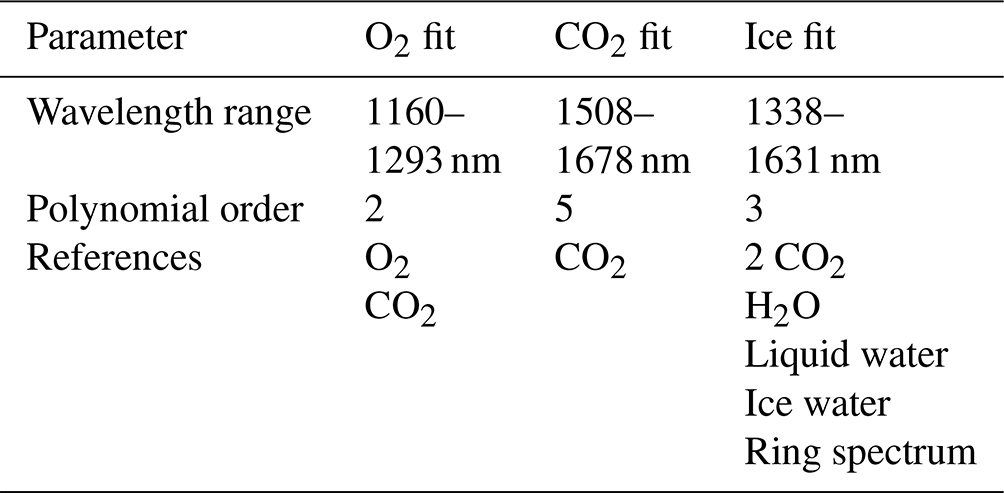
Table 1 List of parameters implemented in the DOAS analysis fit routines.

Absorption cross-sections of ice and liquid water (Warren and Brandt, 2008) do not have narrow structures and were included directly in the fitting process, with the resulting fitting factors then used to derive the ice and liquid water paths (see below).

The retrieval routine determines the scaling factors a_i, and since we use an iterative approach, the path-integrated absorption is the product of a_i (which is always close to 1) and the column density used to calculate the reference spectrum G_j.

To reduce spectral interference between trace gas absorption signatures, we used different spectral windows for the retrievals of ice, O2, and CO₂, each with different model functions, i.e., different combinations of reference spectra (Table 1). The CO2 reference spectra used in the ice fit were made by separating the reference for wavelengths lower than 1498 nm from the portion with wavelengths higher than 1498 nm. The latter portion is then constrained to the amount derived from the CO₂ fit routine. This is done to account for RT differences between the wavelength ranges when ice absorption is high. The ring spectrum in this fit accounts for the effects of Fraunhofer “filling-in” interference signatures caused by rotational Raman scattering and is based on Bussemer (1993). A ring spectrum was found to be unnecessary for fitting O₂ and CO₂ (see Table 1) due to the lack of narrow solar structures.

An example of a retrieval is shown in Fig. 1a, where gas and ice reference spectra (red lines) agree well with the retrieved spectral structures (black lines). The absorption by ice is the strongest spectral signature in this spectrum, with an optical depth of ∼ 0.45. Optical densities of O₂ and CO₂, in the range of 0.03–0.04, are also retrieved with high accuracy.

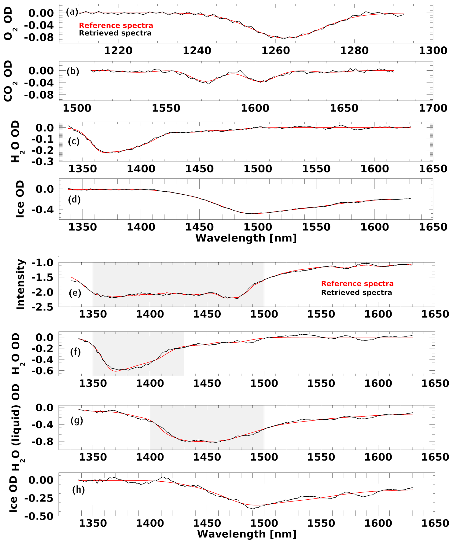
Figure 1 An example of DOAS optical depth fitting, comparing the reference spectra (red lines) of O₂, CO₂, H₂O, and ice. The retrieved spectral structures (black lines) are shown in panels (a), (b), (c), and (d), respectively. A pseudo-saturated case, where strong gas and liquid water absorption flattens the intensity (panel e) signal (shaded areas), making the ice retrieval difficult but still possible, is shown for water and ice in panels (f), (g), and (h).

A complication in the retrievals arises when low-lying liquid water clouds introduce strong water vapor and liquid water absorption (Segelstein, 1981). Panel (b) in Fig. 1 shows an example with a thin liquid water cloud situated below a cirrus ice cloud during Science Flight 2 (SF2). The retrieval is still able to quantify all three phases of water, but a flattening of the intensity between 1350 and 1470 nm due to strong liquid and gaseous water absorption is evident. During parts of the ATTREX flights, these gaseous and liquid water absorptions were even larger than shown here, and some spectra are saturated in this wavelength range. For these cases, we developed a second fit approach where this wavelength interval is omitted. Although this second fit is unable to retrieve water vapor and liquid water, it is still able to determine ice absorption, albeit with larger errors. Due to additional difficulty interpreting these layered-cloud cases with our RT code, we will mostly focus on cases where liquid water absorption is small.

Our gas retrieval routine generates the slant column density (SCD), i.e., the integral of the trace gas concentration along a light path that reaches our instrument:

$$\begin{array}{}\text{(3)}& \mathrm{SCD}=\underset{\mathrm{0}}{\overset{l}{\int }}c\left(s\right)\cdot \mathrm{d}s,\end{array}$$

where c(s) is the gas concentration along the light path. Since the fit must include a solar reference spectrum, which will contain a small amount of trace gas absorption from the atmosphere above the aircraft, the fitting calculates the differential SCD (DSCD), which is the difference between the limb path and solar SCDs:

$$\begin{array}{}\text{(4)}& \mathrm{DSCD}={\mathrm{SCD}}_{\mathrm{limb}}-{\mathrm{SCD}}_{\mathrm{sun}}.\end{array}$$

As we use direct solar light in the absence of overhead clouds, we calculate SCD_sun as an integral of the species along the geometric path from the aircraft to the top of the atmosphere at the time of the solar observation, i.e., using the solar zenith angle (SZA) and flight altitude at the time of measurement. Gas profiles above the aircraft are based on the hypsometric approximation, combined with aircraft observations of temperature and pressure and a stratospheric lapse rate of −2.5 °C km⁻¹. It should be noted that the contribution of SCD_sun is typically less than 2 % and 7 % of SCD_limb for O₂ and CO₂, respectively.

The ice absorption observations from our instrument can be interpreted in a similar way. The ice water path (IWP) is defined as the vertical integral of ice water content through a cloud, a quantity similar to the vertical column density of a trace gas. However, our instrument actually retrieves a slant ice water path (SIWP) defined as

$$\begin{array}{}\text{(5)}& \mathrm{SIWP}=\int {\displaystyle \frac{\mathrm{IWC}}{{\mathit{\rho }}_{\mathrm{ice}}}}\mathrm{d}s,\end{array}$$

where IWC is the ice water content along the light path ds. This equation is a theoretical explanation of what the SIWP represents and also includes ice density ρ_ice to reflect the fact that the absorption coefficient is in units of length (cm⁻¹); consequently, we retrieve the ice light path in units of micrometers (µm) (Fig. 2). It should be noted that the solar reference spectra used in the analysis are measured at the aircraft top altitude under cloud-free conditions, i.e., without ice between the instrument and the sun. Therefore, we do not report a differential SIWP, in contrast to gas retrieval.

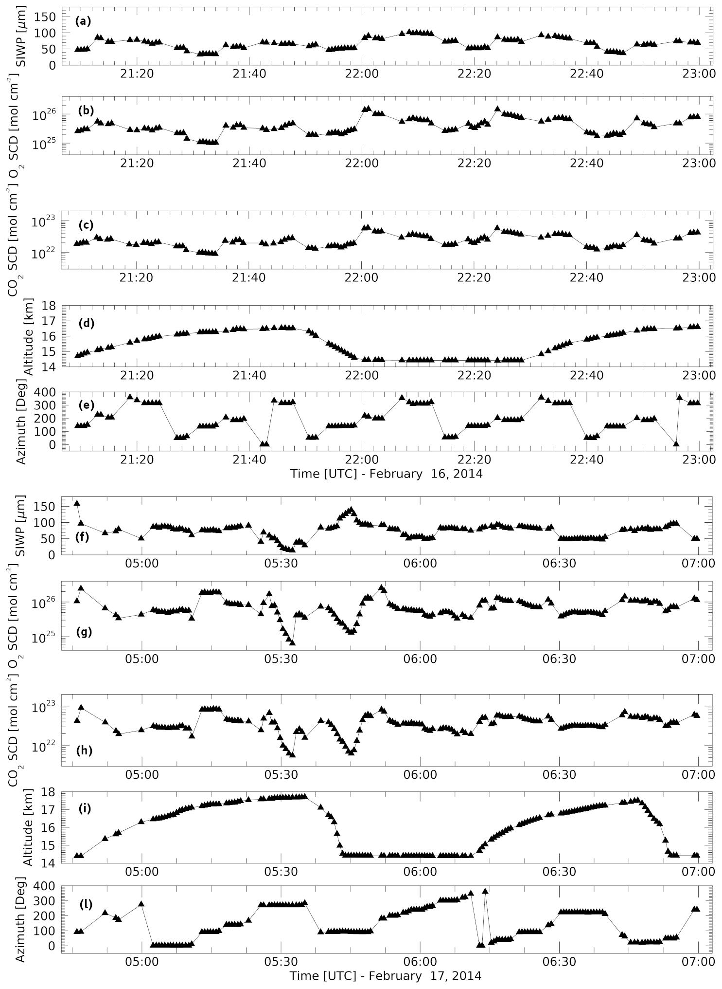
Figure 2 Panels (a), (b), and (c) show the SIWP, O₂, and CO₂ SCD from the first leg of ATTREX SF2 over the ocean near Guam on 16 February 2014. Panels (f), (g), and (h) show the same parameters for the last portion of the flight on 17 February 2014. Water vapor and liquid absorption were low and are not shown here. Panels (d) and (e) and panels (i) and (l) show the flight altitude and the relative azimuth between the solar and viewing directions for the two portions of the flight, respectively. Error bars are similar in size to the symbols and are therefore not included.

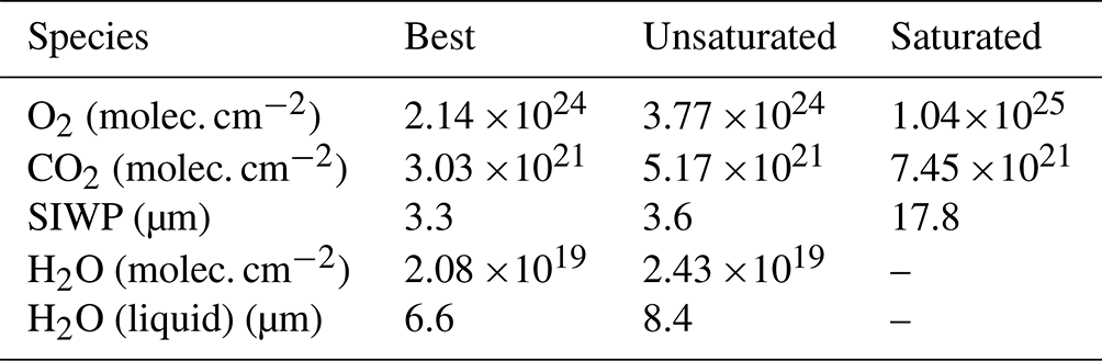
Both the SCDs and the retrieval uncertainties span several orders of magnitude. The retrieval routine calculates an error for each spectrum and detected species. Based on these errors, we have determined that the minimum detection limit is twice the quartile uncertainty in order to remove the influence of higher SCD observations. This may give a better representation of the actual detection limits of the spectrometer. Although the detection limit changed with the observation scenario, the relative uncertainty remained relatively constant for O₂ (3 %), CO₂ (8.2 %), and ice (7.6 %). Unsaturated observations of liquid water and gaseous H₂O had a 10 % and 4.9 % uncertainty, respectively. Consequently, we quote three different retrieval detection limits (Table 2): the best achievable detection limit, the median detection limit at conditions where liquid water absorption is not saturated, and the median detection limit under saturated conditions.

Table 2 Detection limits based on 2σ fit errors.

2.3 ATTREX SF2: a case study

For this study, we focus on a portion of SF2 on 16 February 2014. This flight took place over Guam, a US island territory in Micronesia in the western Pacific (located at 13° N, 144° E), and was characterized by cirrus cloud measurements in a limited area for an extended period of time. This was a uniquely useful flight for the purpose of this study, since the Global Hawk flew rectangular vertical spirals with steep ascending and descending maneuvers, allowing rapid measurements to be taken at different viewing directions and altitudes. Retrievals from SF2 are shown in panels (a) and (b) in Fig. 2, where the change in viewing direction is indicated as the change in the relative azimuth angle between the mini-DOAS viewing direction and the sun (with 0 and 360° indicating that the instrument looks towards the sun and 180° denoting the sun behind the instrument). Lidar and in situ data reveal that, during the ascents and descents (altitude plot in Fig. 2), the aircraft frequently passed through cirrus clouds. The graphs show how O₂ and CO₂ SCDs behaved similarly, confirming our expectation that, since their concentration profiles are constant in time and of similar shape, their behavior is controlled by RT effects. This is also evident from how the SCDs changed with azimuth angle. One conclusion from this observation is that it is sufficient to consider only one of these gases to constrain the RT model. As O₂ retrievals are more accurate and stable, we have focused our analysis on this species.

The retrieved SIWP is in the range of 0–130 µm, showing that the observed light has been impacted by ice particles at all altitudes. The SIWP behavior is also dependent on azimuth, and SIWP tracks the O₂ SCD. In fact, the data retrieved before 23:00 UTC show a reasonably high correlation between the ice absorption and log of O₂ SCD (Pearson correlation coefficient of 0.67). This is somewhat counterintuitive, considering that an increase in ice particle concentration would increase the amount of scattering and thus shorten the O₂ absorption path in the limb. On the other hand, some of the light observed by the instrument originates from below the cloud, where O₂ concentrations are much higher, and enhanced scattering could increase the amount of light from below and thus lead to an increase in O₂. This observation is revisited in Sect. 3.

If we focus on the last part of SF2 (Fig. 2b), we notice that for most of this flight section the SIWP and gas SCDs show the same behavior as for the first part of SF2 (Fig. 2a). However, the period between 05:20 and 05:50 UTC is clearly different. As the Global Hawk climbs above 17 km altitude, around 05:20 UTC, the SIWP drops to near-zero values. At the same time O₂ and CO₂ SCDs also drop to very low values. We interpret this behavior to arise from observations above a thick cirrus cloud, where no or few ice particles are within the observation volume. The remaining nonzero SIWP comes from upwelling light from the cirrus cloud that is then scattered by air molecules into the line of sight (LOS) of the instrument. The cloud also seems to block light from lower parts of the atmosphere so that the gas SCDs arise solely from absorption within the (limb) line of sight and from above. The subsequent descent into this thick cloud also leads to the highest SIWP observed in this flight. The peak in SIWP is accompanied by an anticorrelated decrease in O₂ and CO₂ SCDs, likely caused by the fact that the cirrus cloud is optically very thick and most of the observed light originates from scattering by ice particles rather than from air molecules. Again, no light from the lower atmosphere reaches the instrument.

These examples clearly show that measured O₂ and ice absorption are impacted by cirrus cloud geometry, solar zenith angle, viewing zenith angle, azimuth angle, flight altitude, and other geometrical and physical factors. This motivates the need for RT model calculations to properly interpret ice absorption measurements under a variety of different conditions. As part of this study we therefore developed an expanded version of the VLIDORT radiative transfer code (Spurr, 2006), capable of handling limb geometries.

2.4 Radiative transfer model

The VLIDORT-QuasiSpherical (VLIDORT-QS) vector RT model (Spurr et al., 2022) was used to simulate the ATTREX observations and to perform the sensitivity tests. Based on the recent version 2.7 (released early 2015) of the VLIDORT code (Spurr, 2006), the completely new VLIDORT-QS code was specifically designed and developed for the interpretation of high-altitude limb-scanning measurements. Ray tracing in a fully spherical atmosphere is a crucial capability for the simulation of ATTREX measurements, which are made in the limb at 14–20 km altitude with absorption path lengths of up to 300 km. To account for various viewing angles (the up-, down-, or limb-viewing regimes), the model must be able to perform RT calculations along all fully illuminated (no shadow or twilight conditions are currently considered) line-of-sight (LOS) paths.

The Earth's atmosphere is quite strongly curved. In order to obtain sufficient accuracy for scenarios such as those for ATTREX, where long paths through the atmosphere are present, it is necessary to perform RT in a curved spherical-shell atmosphere for both the single scatter (SS) and the multiple scatter (MS) contributions to the radiation field. To this end, VLIDORT-QS relies on a spherical-shell optical model, comprising a series of optically uniform layers extending from the surface to the TOA with resolution 1–2 km in the troposphere and 0.5 km in the upper troposphere–lower stratosphere, where the ATTREX measurements were taken. VLIDORT-QS assumes horizontal uniformity of the atmosphere. For the SS component, VLIDORT-QS solves the RT equation (RTE) accurately for each path segment in a curved-shell atmosphere for any of the regimes noted above. A given segment SS source term is established by integrating the SS RTE numerically from segment start to finish, using a Gauss–Legendre quadrature scheme defined by N_j points of abscissa and weights {α_j,χ_j} ($j=\mathrm{1},\mathrm{2},\mathrm{\dots },N_j$), based on the change of LOS zenith angle α. These segment quadrature points define an intermediate set of solar angles {θ_j}, for which solar-beam ray tracing is performed, plus a corresponding set of vertical optical thicknesses {τ_j}. Once the layer SS source terms are found, the radiation field at the observer's position is developed recursively, starting with the value at the path origin (TOA or surface) and using the cumulative LOS transmittances to propagate these source terms. Path segments are mostly defined by layer boundaries, except for those segments in the limb view on either side of the tangent point. If the observer is placed between two layer boundaries, then the final segment of the LOS will encompass a partial layer.

For the MS component, the code relies on an adapted form of the VLIDORT RT model in which a single call to VLIDORT for each segment will generate a set of plane-parallel discrete-ordinate solutions to the RTE at each of quadrature points {α_sj,χ_sj} ($j=\mathrm{1},\mathrm{2},\mathrm{\dots },N_j$ in that segment). The MS segment source term is then derived by integrating these MS solutions using the same quadrature scheme as was used for the SS field. In essence, the plane-parallel source function integration scheme normally employed in VLIDORT is replaced by a scheme done in full spherical geometry. This is in some ways equivalent to a piece-wise concatenation of MS 1-D RT solutions in a 3-D scenario. VLIDORT-QS is not a truly spherical model; it cannot deal with Earth-shadow scenarios and is confined to geometrical configurations in which all points on the LOS path are fully illuminated (no incident-beam twilight situations, solar zenith angles must be less than 90°). However, all MS solutions from VLIDORT are obtained in the pseudo-spherical approximation, in which solar beam attenuation (before scattering) is always treated accurately for a curved atmosphere.

An accurate and comprehensive theoretical description of the new VLIDORT-QS RT code is provided in Spurr et al. (2022), where the RT code is validated against the standard VLIDORT model for nadir-view (low sphericity) scenarios and against the fully spherical Monte Carlo MYSTIC model (Emde et al., 2016) (part of LibRadTran RT code package; Mayer and Kylling, 2005) for cases with higher sphericity. The validation includes general near-IR simulations for high-altitude aircraft limb- and nadir-viewing scenarios, including a Rayleigh-only regime, and in the presence of stratospheric clouds for different observational altitudes, viewing angles, and surface albedo. Results of these tests showed average differences among the RT codes on the order of a few percent, depending on the geometry and the scenario.

2.5 ATTREX RT calculations

In order to simulate realistic cirrus cloud environments, we replicated the general conditions of the ATTREX scenarios, as encountered on 16 February 2014 during SF2. The atmosphere was divided into 50 layers, with a pressure range from 1015.3 mbar (surface) to 9.4 mbar (TOA) and an altitude range between 0 and 32 km. The vertical grid spacing was set to 1 km between 0–10 km and 0.5 above 10 km altitude. Temperature, pressure, and molecular and scattering particle properties are considered to be homogeneous within each layer. In the near-IR spectral range (900–1800 nm), the main atmospheric absorbers are O₂, CO₂, and H₂O. Because of the low atmospheric pressure due to the measurement altitude, the quadratic contribution at 1067 and 1270 nm due to the absorption induced by the O₂–O₂ collision (Smith and Newnham, 1999) has not been considered in this study. Vertical profiles of O₂ and CO₂ are calculated using fixed mixing ratios of 0.21 and 370 ppm, respectively. The surface is assumed to be Lambertian. No lower-atmospheric clouds were considered in the model. We used a flight altitude of 16.5 km for our sensitivity tests, unless otherwise noted, and the true aircraft altitude for retrievals. The ice cloud deck was located between 14 and 18 km for all tests.

The ice particle optical properties were determined from averaged in situ data provided by the CPI and FCDP instruments (described in Sect. 2) as part of the Global Hawk payload. Images from the CPI provided information about the habit classification, while FCDP measurements yielded the number concentration as a function of particle size. It is worth notice that the FCDP instrument measures particles between 1 and 50 µm, defining the size interval for the microphysical properties used in the ice retrievals from the DOAS observations.

During SF2, the aircraft sampled the same area for an extended period of time. However, ice particle numbers varied widely. We therefore calculated an averaged ice particle number concentration over the period of interest for this study and used this to calculate the relative total volume. Knowing the density of ice ${\mathit{\rho }}_{\mathrm{ice}}=\mathrm{0.91}\times {\mathrm{10}}^{\mathrm{6}}$ g m⁻³, this resulted in an ice water content of IWC${}_{\mathrm{0}}=\mathrm{1.22}\times {\mathrm{10}}^{-\mathrm{3}}$ g m⁻³. If not otherwise specified, IWC₀ is referred to as the nominal case in the rest of the paper. This value represents the baseline, and the different ice water contents used in this study are expressed as multiplicative factors with respect to the nominal value.

Although classical Mie theory is not ideally suited for deriving optical properties of clouds with nonspherical ice particles, images from the Hawkeye CPI data showed that the ice particles were largely quasi-spherical for the smaller particles size range covered by the FCDP instrument (Woods et al., 2018), and we have accordingly used Mie theory for the calculation of these properties. Furthermore, as will become clear in the subsequent discussion, an overall understanding of the principles of limb ice absorption measurements is not in general impacted by the shape of the particles.

Since scattering from ice particles enhances simulated limb radiances (making the intensity in the absence of ice actually smaller than that in the presence of ice), a differential approach for the ice absorption simulation was implemented, wherein the ice absorption was evaluated using the intensity at two different wavelengths λ₁ and λ₂ according to

$$\begin{array}{}\text{(6)}& {\mathit{\tau }}_{\mathrm{ice}}=\ln \left[{\displaystyle \frac{I_{\mathit{\lambda }\mathrm{1}}^{\mathrm{0}}}{I_{\mathit{\lambda }\mathrm{2}}^{\mathrm{0}}}}\right]-\ln \left[{\displaystyle \frac{I_{\mathit{\lambda }\mathrm{1}}}{I_{\mathit{\lambda }\mathrm{2}}}}\right],\end{array}$$

where the pairs $I_{\mathit{\lambda }\mathrm{1}}^{\mathrm{0}}$–$I_{\mathit{\lambda }\mathrm{2}}^{\mathrm{0}}$ and I_λ1–I_λ2 indicate the intensities in the absence and presence of ice for the two selected wavelengths, respectively. It should be noted that this approach is similar to that underlying the differential absorption retrieval described above. Wavelengths of 1548.1 and 1550.3 nm, at the edges of a broad ice absorption feature, were selected for λ₁ and λ₂, respectively. Gas absorption lines are weak at these wavelengths, thus reducing any effect that gas absorption has on ice particle scattering. Oxygen absorption, on the other hand, was calculated according to Beer's law:

$$\begin{array}{}\text{(7)}& {\mathit{\tau }}_{{\mathrm{O}}_{\mathrm{2}}}=\ln \left[{\displaystyle \frac{I_{\mathit{\lambda }}^{\mathrm{0}}}{I_{\mathit{\lambda }}}}\right],\end{array}$$

where gaseous optical absorption is evaluated as the logarithmic ratio between intensities calculated with and without the absorber, I_λ and $I_{\mathit{\lambda }}^{\mathrm{0}}$, respectively. In this study, oxygen absorption was calculated at λ=1260.8 nm using two consecutive runs of the model (with and without oxygen absorption).

3 Sensitivity studies for ice absorption in cirrus clouds

Observations during ATTREX revealed that both ice and oxygen absorptions are highly variable, not only due to the presence of varying amounts of ice, but also due to different solar geometries and altitudes. The first goal of this study was therefore to develop a fundamental understanding of the mechanism and dependencies of ice scattering and absorption in cirrus clouds under near-limb viewing conditions using sensitivity studies for ice and oxygen absorption under various conditions (Table 3).

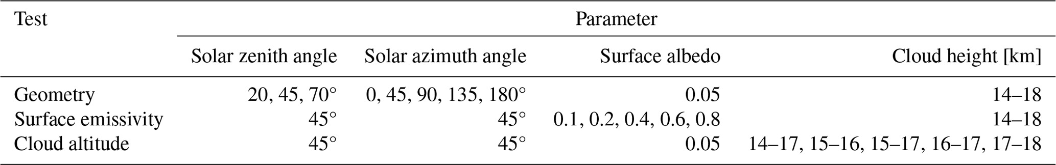
Table 3 The table lists the parameters used for the three different sensitivity tests (geometry, surface emissivity, and cloud altitude test) performed. For example, the geometry test has a fixed surface albedo (0.05) and cloud extension (14–18 km), and only solar and azimuth angles are varied, according to the value in the corresponding cell. Flight altitude is set to 16.5 km for all tests.

For each sensitivity test, the ice mass concentration was varied by scaling IWC₀ over 5 orders of magnitude, representative of typical ice mass concentrations from thin to thick cirrus clouds (Krämer et al., 2016).

All tests showed a similar general behavior as the ice mass concentration was varied. Ice absorbance, i.e., SIWP, shows a linear dependence on ice mass concentration for scaling factors below IWC${}_{\mathrm{0}}\times {\mathrm{10}}^{-\mathrm{1}}$ (Fig. 3a, c, and e). Oxygen absorbance remains constant in this range (Fig. 3b, d, and f). For ice mass concentrations above the nominal IWC₀, ice absorbance begins to flatten, while oxygen begins to deviate from its constant value at low concentrations below IWC₀. This transition depends on the solar geometry as will be discussed in further detail below.

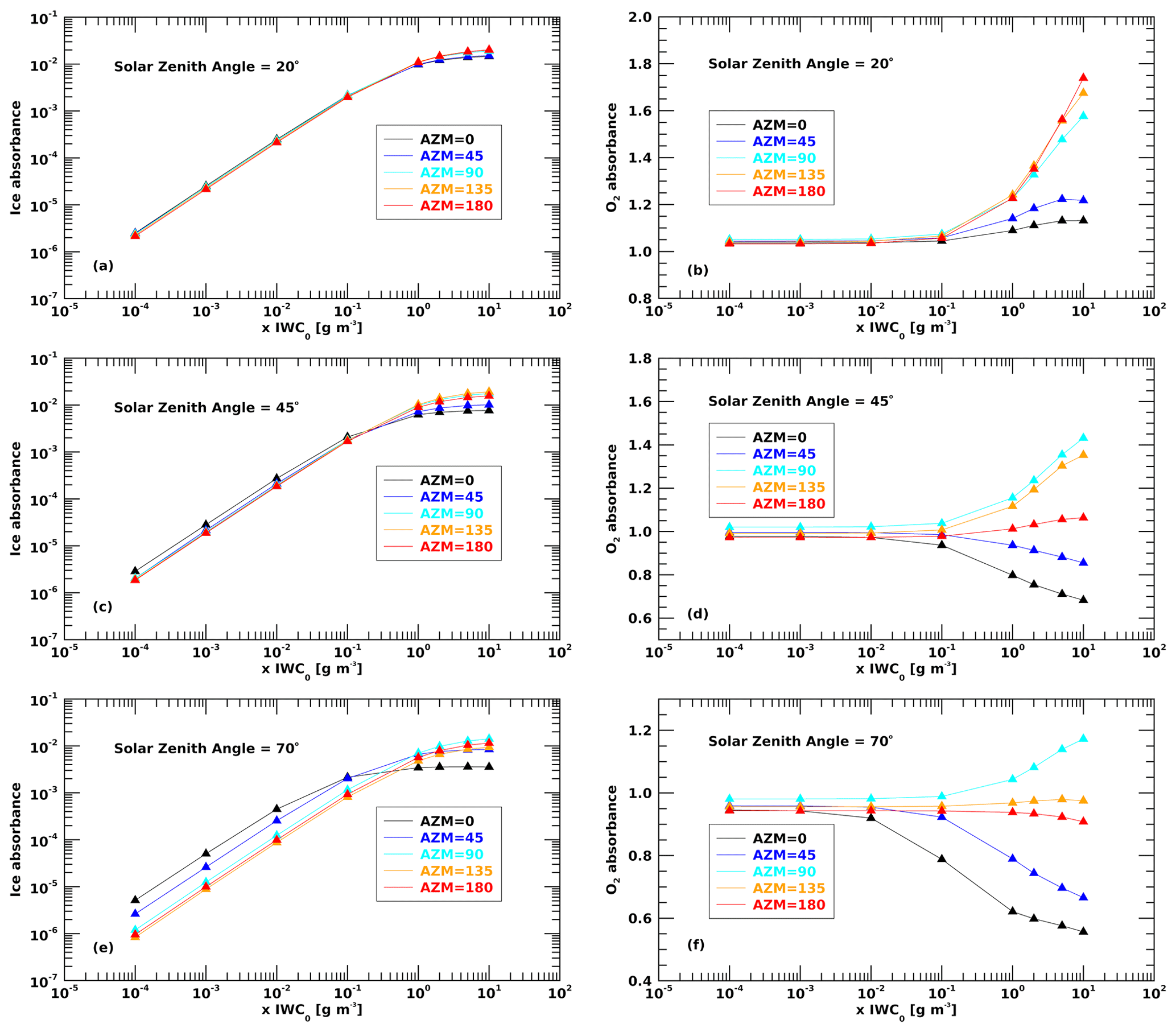
Figure 3 Ice absorbance (left column) and O₂ absorbance at five azimuth angles (0, 45, 9, 135, and 180°) and for three different solar zenith angles (20, 45, and 70°) as a function of ice particle mass concentration. The x-axis values represent the different ice mass concentrations, expressed as multiplicative factors with respect to the nominal value IWC₀ (i.e., 10⁰ = IWC₀, 10⁻¹ = 0.1× IWC₀, ...).

To study the transition from a linear to a nonlinear ice absorption regime, we separated the SS and MS contributions to the model output intensities (Fig. 4). It should be noted here that the MS contribution in VLIDORT-QS includes radiation diffusely reflected by the surface and the atmosphere below the aircraft. The low ice mass concentration regime is described by a constant $\mathrm{MS}/\mathrm{SS}$ intensity ratio. This ratio is nonzero due to the surface scattering and reflection contribution. MS becomes more important at the transition point. However, the $\mathrm{MS}/\mathrm{SS}$ ratio remains below 2 %, indicating that MS only plays a minor role in the flattening of the ice absorption signature and that SS dominates overall.

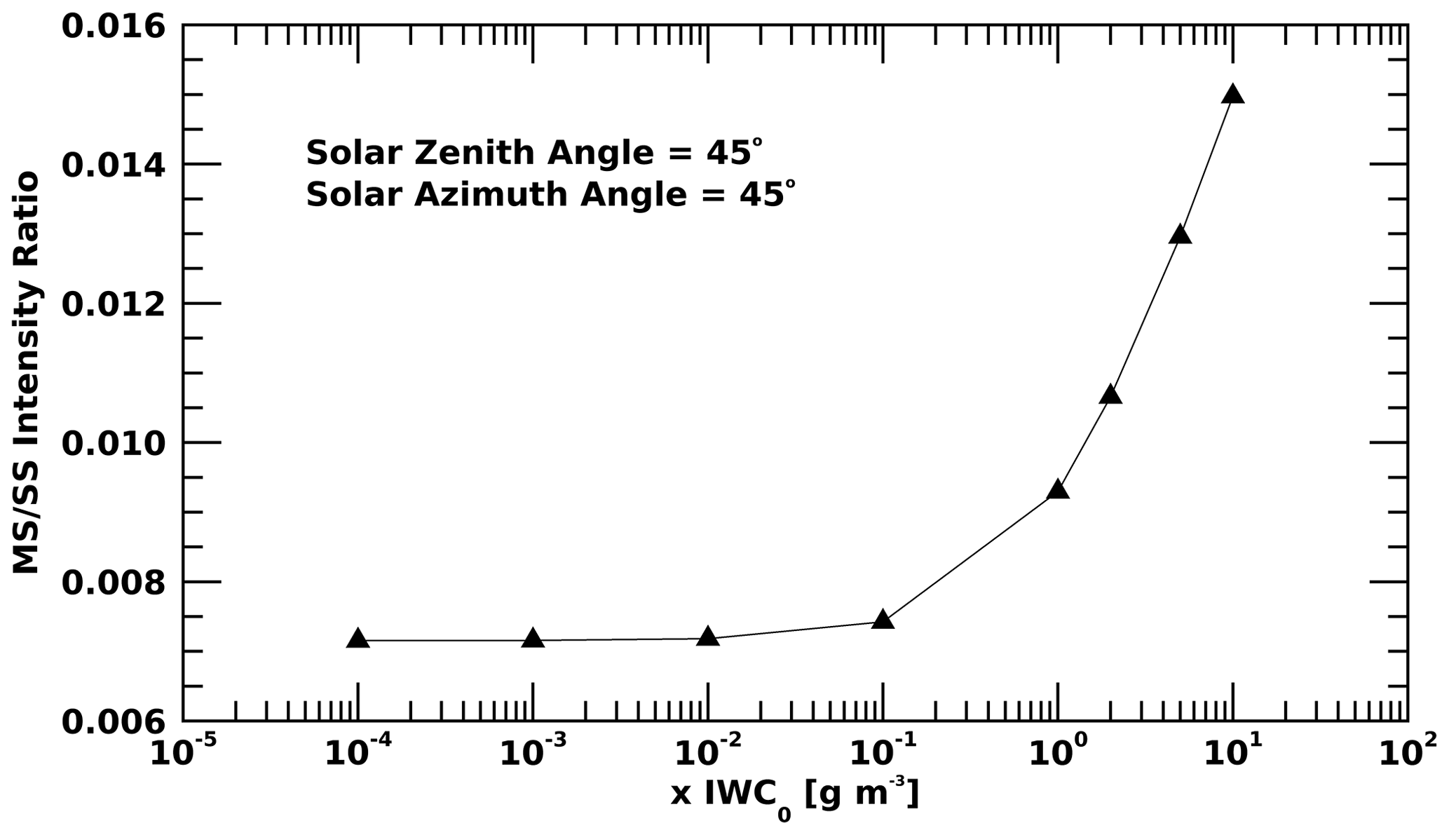
Figure 4 Ratio of the contribution of SS and MS intensities as a function of ice mass concentration.

The linear dependence of ice absorbance is thus a consequence of the increased scattered radiance as a function of the greater number of particles. The lack of sensitivity of oxygen absorbance at low ice mass concentrations can be explained by the small contribution that ice particle scattering has to the overall radiance compared to scattering by air molecules in this regime. In the transition regime, the ice particle scattering contribution increases, thus making the gas absorbance more sensitive to lower parts of the atmosphere, ice particle optical properties, and sun geometry.

To better understand the impact of solar geometry, we simulated ice and O₂ absorption for five different azimuth angles (SAZ: 0, 45, 90, 135, 180°) and for three solar zenith angles (SZA: 20, 45, 70°). The basic shape of the ice absorption curves remains similar for all sun geometries (Fig. 3). The ice mass concentration at which the transition from linear to nonlinear behavior occurs and the slope in the nonlinear regime both depend on SAZ and SZA. In the low ice mass concentration regime, larger ice absorption occurs at lower SAZ (viewing towards the sun), while at larger SAZ there is a systematic decrease in the ice absorption, reaching a minimum when the sun is opposite to the instrument LOS. Interestingly, this pattern is reversed at higher ice mass concentrations: lower ice absorption is now associated with smaller SAZ, and an increase in SAZ returns to higher ice absorption.

This effect can be partially explained by strong forward scattering of the ice particles. Radiation is predominantly scattered along the direction of the incoming beam, while most of the absorption occurs along the instrument LOS. Conversely, backscattered radiation observed at higher SAZ provides less absorption in the direction of the instrument LOS. The reversal at higher ice mass concentrations is likely due to more complex radiative effects, such as a higher contribution of the observed skylight radiance stemming from ice compared to air or the increased contribution of MS. The dependence on SZA is particularly evident for SZA = 20° (Fig. 3a), where ice absorption differences are reduced by the small SZA (no azimuthal dependence of the ice absorption at the zenith). At SZA = 70° (Fig. 3e), the longer atmospheric absorption path makes the effect of the SAZ more pronounced. The O₂ absorption behavior, for the same change in observational geometry, shows that at low ice mass concentrations the absorption is basically constant, while it diverges in the high-ice-mass-concentration regime. The more complex response of O₂ absorbance at high ice mass concentration is explored in more detail below.

Limb measurements at high altitudes can be affected by radiation reflected by the surface. Consequently, a sensitivity test was performed for different surface reflectivities in order to evaluate the influence of the surface albedo on the measurements (Fig. 5). We varied the albedo from 0.1 to an unrealistic value of 0.8 to clearly demonstrate the effect of the surface. Radiation from the surface contributes an additional term to the signal, proportional to the percentage of light reflected back into the atmosphere. Both ice and oxygen absorbances increase linearly with the albedo, showing this scaling effect.

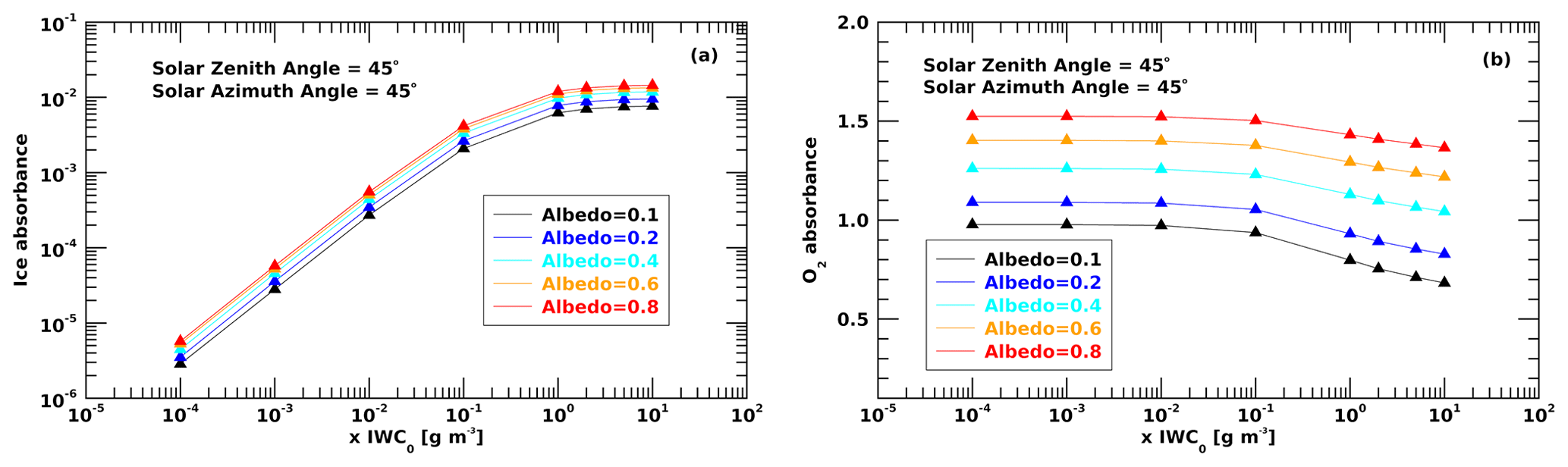
Figure 5 Ice (a) and O₂ (b) absorbance as a function of ice mass concentration for four different surface albedos (0.1. 0.2, 0.4, 0.6, 0.8). Simulations were performed for SZA = 45° and SAZ = 45°.

In order to investigate the effect of different cloud altitudes on the signal, we compared simulations for five different cloud geometries (14–17, 15–16, 15–17, 16–17, and 17–18 km), keeping the flight altitude constant at 16.5 km. This allowed us to simulate conditions close to those for the actual measurements, whereby the instrument is flying below, inside, and above ice clouds (Fig. 6). Simulations of ice absorbance for observations inside and below the cloud behave similarly, while measurements above the cloud resulted in much lower ice absorbance. In the latter case, the instrument collects photons coming mainly from the thin atmosphere above the cloud. When the aircraft is below the cloud (17–18 km case in Fig. 6), most of the signal originates from the atmosphere below the aircraft, but solar radiation first passes through the cloud and is then scattered below it, contributing to a similar pattern present in observations taken inside the cloud.

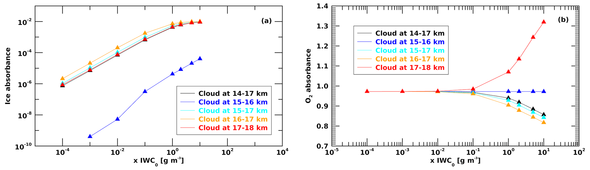
Figure 6 Cloud altitude sensitivity simulations of ice (a) and O₂ (b) absorbance for five different cases at 14–17, 15–16, 15–17, 16–17, and 17–18 km to simulate measurements above, inside, and below the cloud deck. Flight altitude is fixed at 16.5 km.

The oxygen absorbance behaves as expected (Fig. 6), with no dependence on cloud geometry at low ice mass concentrations. At higher ice mass concentrations, when the instrument observes above the cloud (cloud located between 15 and 16 km), the oxygen absorbance remains constant, as photons only originate from above the cloud. Simulations for observation inside the cloud show that the oxygen absorbance decreases with ice mass concentration as the oxygen absorption path shortens. When the aircraft is below the cloud (located at 17–18 km), an increase in ice mass concentration (thicker cloud) enhances the signal as a consequence of an increased contribution of the oxygen absorption in the lower part of the atmosphere.

Conceptual model of high-altitude limb ice and oxygen absorptions

These sensitivity studies reveal a number of common features in limb observations of SIWP (ice absorbance) and O₂ SCD in cirrus clouds.

• At low ice mass concentration, SIWP is a linear function of ice mass concentration, while oxygen SCD remains constant.

• At high ice mass concentrations, SIWP levels off, while oxygen SCD decreases or increases depending on viewing geometry.

• SIWP and O₂ SCD are functions of viewing geometry. In particular the O₂ SCD at high ice mass concentration is highly dependent on the viewing azimuth angle.

• SIWP and O₂ SCD are both functions of surface (and lower clouds) albedo.

• SIWP and O₂ SCD are both functions of cloud geometry and relative observation altitude.

The first four items in this list allow us to develop a general understanding of our observations. To this end, we have used a simplified description of the source of light observed by the limb-viewing mini-DOAS system. Despite their intrinsic difference, the terms optical depth and absorption are considered synonymous throughout the paper because both relate to O₂ SCD and SIWP.

As illustrated in Fig. 7, the observed skylight radiance can be approximated by the sum of four different components. $I_{\mathrm{S}}^R$ is the radiance of sunlight scattered by air molecules. $I_{\mathrm{S}}^M$ is the radiance of sunlight scattered by ice particles. $I_{\mathrm{A}}^R$ and $I_{\mathrm{A}}^M$ are the radiances of upwelling light, i.e., sunlight scattered upward by the surface and the atmosphere (air molecules and ice particles), respectively. These quantities can be written as follows.

$$\begin{array}{}\text{(8)}& {\displaystyle }{I}_{\mathrm{S}}^R\left(\mathit{\lambda }\right)=I_{\mathrm{S}}\left(\mathit{\lambda }\right)\cdot P_{\mathrm{S}}^R(\mathit{\theta },\mathit{\vartheta },\mathit{\lambda })\cdot {\mathit{ϵ}}_R\left(\mathit{\lambda }\right)\cdot C_{\mathrm{air}}\text{(9)}& {\displaystyle }{I}_{\mathrm{S}}^M\left(\mathit{\lambda }\right)=I_{\mathrm{S}}\left(\mathit{\lambda }\right)\cdot P_{\mathrm{S}}^M(\mathit{\theta },\mathit{\vartheta },\mathit{\lambda })\cdot {\mathit{ϵ}}_M\left(\mathit{\lambda }\right)\cdot N_{\mathrm{ice}}\text{(10)}& {\displaystyle }{I}_{\mathrm{A}}^R\left(\mathit{\lambda }\right)=I_{\mathrm{S}}\left(\mathit{\lambda }\right)\cdot R\left(\mathit{\lambda }\right)\cdot P_{\mathrm{A}}^R(\mathit{\theta },\mathit{\vartheta },\mathit{\lambda })\cdot {\mathit{ϵ}}_R\left(\mathit{\lambda }\right)\cdot C_{\mathrm{air}}\text{(11)}& {\displaystyle }{I}_{\mathrm{A}}^M\left(\mathit{\lambda }\right)=I_{\mathrm{S}}\left(\mathit{\lambda }\right)\cdot R\left(\mathit{\lambda }\right)\cdot P_{\mathrm{A}}^M(\mathit{\theta },\mathit{\vartheta },\mathit{\lambda })\cdot {\mathit{ϵ}}_M\left(\mathit{\lambda }\right)\cdot N_{\mathrm{ice}}\end{array}$$

Here I_S(λ) represents the incoming solar intensity, $P(\mathit{\theta },\mathit{\vartheta },\mathit{\lambda })$ represents the phase function for scattering events, R(λ) is a factor taking into account the radiation reflected by the surface and atmosphere below the aircraft, ϵ_R(λ) and ϵ_M(λ) represent the Rayleigh and Mie extinctions, respectively, C_air is the concentration of air molecules, and N_ice identifies the ice particle mass concentration. Using the following representation of the observed radiance,

$$\begin{array}{}\text{(12)}& I_{\mathrm{obs}}\left(\mathit{\lambda }\right)=I_{\mathrm{S}}^R\left(\mathit{\lambda }\right)+I_{\mathrm{S}}^M\left(\mathit{\lambda }\right)+I_{\mathrm{A}}^R\left(\mathit{\lambda }\right)+I_{\mathrm{A}}^M\left(\mathit{\lambda }\right),\end{array}$$

and remembering Eq. (7), we can now use these equations to describe the generic optical depth at wavelength λ as

$$\begin{array}{}\text{(13)}& \begin{array}{rl}{\mathit{\tau }}_{\mathit{\lambda }}& =-\ln \left[\left(P_{\mathrm{S}}^R\right(\mathit{\lambda })+R(\mathit{\lambda })\cdot P_{\mathrm{A}}^R(\mathit{\lambda }\left)\right)\cdot {\mathit{ϵ}}_R\left(\mathit{\lambda }\right)\right.\\ & \left.\cdot C_{\mathrm{air}}+\left(P_{\mathrm{S}}^M\left(\mathit{\lambda }\right)+R\left(\mathit{\lambda }\right)\cdot P_{\mathrm{A}}^M\left(\mathit{\lambda }\right)\right)\cdot {\mathit{ϵ}}_M\left(\mathit{\lambda }\right)\cdot N_{\mathrm{ice}}\right]\\ & =-\ln \left[A\cdot {\mathit{ϵ}}_R\left(\mathit{\lambda }\right)\cdot C_{\mathrm{air}}+B\cdot {\mathit{ϵ}}_M\left(\mathit{\lambda }\right)\cdot N_{\mathrm{ice}}\right]\\ & =-\ln (A\cdot {\mathit{ϵ}}_R(\mathit{\lambda })\cdot C_{\mathrm{air}})-\ln \left[\mathrm{1}+{\displaystyle \frac{B\cdot {\mathit{ϵ}}_M\left(\mathit{\lambda }\right)\cdot N_{\mathrm{ice}}}{A\cdot {\mathit{ϵ}}_R\left(\mathit{\lambda }\right)\cdot C_{\mathrm{air}}}}\right],\end{array}\end{array}$$

where we have introduced $A=P_{\mathrm{S}}^R\left(\mathit{\lambda }\right)+R\left(\mathit{\lambda }\right)\cdot P_{\mathrm{A}}^R\left(\mathit{\lambda }\right)$ and $B=P_{\mathrm{S}}^M\left(\mathit{\lambda }\right)+R\left(\mathit{\lambda }\right)\cdot P_{\mathrm{A}}^M\left(\mathit{\lambda }\right)$ to simplify the equation. A and B are functions of the geometry, the radiation reflected by the surface and atmosphere below the aircraft, and the scattering properties of air (function A) and ice particles (function B), respectively. These general expressions for the optical depth can be approximated for two special cases (low and high ice mass concentrations) for oxygen and ice, depending on the different relative weights of the two terms in Eq. (13):

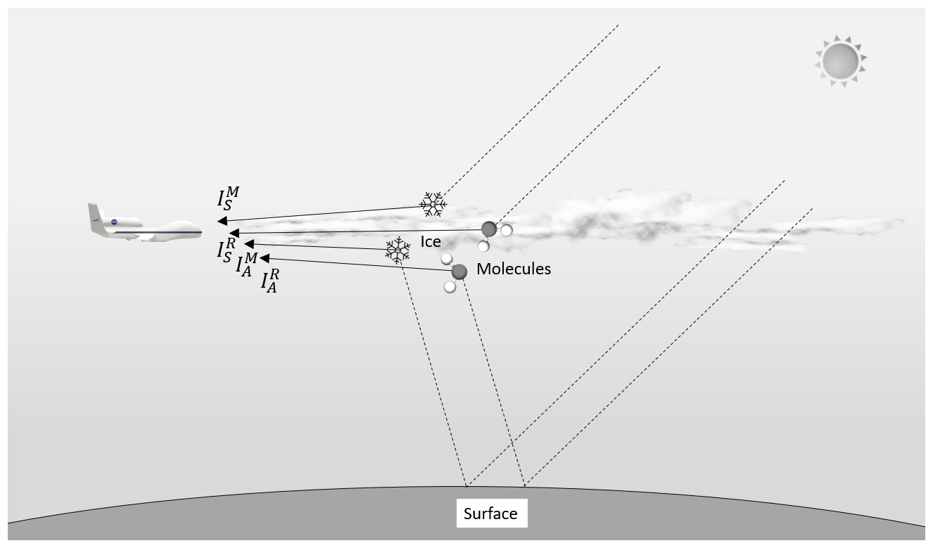
Figure 7 Sketch of the radiative quantities defining the observed radiance: $I_{\mathrm{S}}^R$ is the component of sunlight scattered by air molecules, $I_{\mathrm{S}}^M$ is the component of sunlight scattered by ice particles, and $I_{\mathrm{A}}^R$ and $I_{\mathrm{A}}^M$ are the radiances of upwelling light, after the interaction with the surface, due to molecules and particles, respectively.

Case I: low ice mass concentration

$$\begin{array}{}\text{(14)}& A\cdot {\mathit{ϵ}}_R\left(\mathit{\lambda }\right)\cdot C_{\mathrm{air}}\gg B\cdot {\mathit{ϵ}}_M\left(\mathit{\lambda }\right)\cdot N_{\mathrm{ice}}\end{array}$$

In this case, invoking ln$(\mathrm{1}+x)\approx x$ for x≈0, Eq. (13) can be approximated as

$$\begin{array}{}\text{(15)}& {\mathit{\tau }}_{\mathit{\lambda }}\approx -\ln (A\cdot {\mathit{ϵ}}_R(\mathit{\lambda })\cdot C_{\mathrm{air}})-\left({\displaystyle \frac{B\cdot {\mathit{ϵ}}_M\left(\mathit{\lambda }\right)}{A\cdot {\mathit{ϵ}}_R\left(\mathit{\lambda }\right)\cdot C_{\mathrm{air}}}}\right)\cdot N_{\mathrm{ice}}.\end{array}$$

The ice optical depth is calculated as a differential absorption (Eq. 6) at two adjacent wavelengths λ₁ and λ₂.

$$\begin{array}{}\text{(16)}& {\mathit{\tau }}_{\mathrm{ice}}=\ln \left[{\displaystyle \frac{I_{\mathit{\lambda }\mathrm{1}}^{\mathrm{0}}}{I_{\mathit{\lambda }\mathrm{2}}^{\mathrm{0}}}}\right]-\ln \left[{\displaystyle \frac{I_{\mathit{\lambda }\mathrm{1}}}{I_{\mathit{\lambda }\mathrm{2}}}}\right]={\mathit{\tau }}_{{\mathit{\lambda }}_{\mathrm{1}}}-{\mathit{\tau }}_{{\mathit{\lambda }}_{\mathrm{2}}}\end{array}$$

The proximity of the chosen wavelengths allows us to take A(λ₁)≈A(λ₂), and we can further assume that ϵ_M(λ₁)≈ϵ_M(λ₂) because of the relatively weak dependence of Rayleigh extinction on wavelength in the ice absorption range. The combination of Eqs. (15) and (16) leads to a compact expression for ice absorption for low ice mass concentration.

$$\begin{array}{}\text{(17)}& {\mathit{\tau }}_{\mathrm{ice}}^{\mathrm{low}}\approx -{\displaystyle \frac{B\left({\mathit{\lambda }}_{\mathrm{1}}\right)\cdot {\mathit{ϵ}}_M\left({\mathit{\lambda }}_{\mathrm{1}}\right)-B\left({\mathit{\lambda }}_{\mathrm{2}}\right)\cdot {\mathit{ϵ}}_M\left({\mathit{\lambda }}_{\mathrm{1}}\right)}{A\cdot {\mathit{ϵ}}_R\cdot C_{\mathrm{air}}}}\cdot N_{\mathrm{ice}}\end{array}$$

Equation (17) clearly demonstrates that under conditions where scattering by air molecules outweighs that by ice particles, a linear dependence of ice absorption (SIWP) on the ice mass concentration is expected, with a proportionality factor that depends on the ice-scattering phase function.

This result now raises the question of why the oxygen absorption seems independent of N_ice in our sensitivity tests. For the O₂ absorption, Eq. (15) can be simply approximated as

$$\begin{array}{}\text{(18)}& {\mathit{\tau }}_{{\mathrm{O}}_{\mathrm{2}}}^{\mathrm{low}}\approx -\ln \left(A\cdot {\mathit{ϵ}}_R\left(\mathit{\lambda }\right)\cdot C_{\mathrm{air}}\right),\end{array}$$

which explains the lack of sensitivity of oxygen absorbance at low ice mass concentrations. In this expression, the function A is large and is independent of N_ice.

Equations (17) and (18) explain the behavior of O₂ and ice absorption in our RTM sensitivity tests at low ice mass concentrations and thus provide a conceptual model for this regime.

Case II: high ice mass concentration

$$\begin{array}{}\text{(19)}& A\cdot {\mathit{ϵ}}_R\left(\mathit{\lambda }\right)\cdot C_{\mathrm{air}}\ll B\cdot {\mathit{ϵ}}_M\left(\mathit{\lambda }\right)\cdot N_{\mathrm{ice}}\end{array}$$

In this second special case, all of the previous approximations are no longer valid, and the optical depth is described again by Eq. (13), which, after combining with Eq. (16), leads to a new expression for the ice absorption.

$$\begin{array}{}\text{(20)}& \begin{array}{rl}{\mathit{\tau }}_{\mathrm{ice}}^{\mathrm{high}}& \approx -\ln \left[{\displaystyle \frac{A\cdot {\mathit{ϵ}}_R\cdot C_{\mathrm{air}}+B\left({\mathit{\lambda }}_{\mathrm{1}}\right)\cdot {\mathit{ϵ}}_M\left({\mathit{\lambda }}_{\mathrm{1}}\right)\cdot N_{\mathrm{ice}}}{A\cdot {\mathit{ϵ}}_R\cdot C_{\mathrm{air}}+B\left({\mathit{\lambda }}_{\mathrm{2}}\right)\cdot {\mathit{ϵ}}_M\left({\mathit{\lambda }}_{\mathrm{2}}\right)\cdot N_{\mathrm{ice}}}}\right]\\ & \propto -\ln \left[{\displaystyle \frac{B\left({\mathit{\lambda }}_{\mathrm{1}}\right)\cdot {\mathit{ϵ}}_M\left({\mathit{\lambda }}_{\mathrm{1}}\right)}{B\left({\mathit{\lambda }}_{\mathrm{2}}\right)\cdot {\mathit{ϵ}}_M\left({\mathit{\lambda }}_{\mathrm{2}}\right)}}\right]\end{array}\end{array}$$

This explains why SIWP becomes independent of ice mass concentration N_ice but at the same time remains strongly dependent on the viewing geometry and ice phase function, which is included in B(λ). The factor B(λ) also contains the factor R (Eqs. 10 and 11), which includes the surface albedo. Consequently, ice absorbance at high ice mass concentrations depends in a complex way on the sun geometry and the phase functions at different wavelengths, as well as the atmosphere and surface below the cloud. Further exploration of this regime thus requires detailed simulations with a proper RTM.

For oxygen absorption, Eq. (6) is unable to fully describe the behavior seen in Fig. 3, although the strong dependence on the viewing geometry, ice phase function, and atmosphere and surface through the term B(λ) can partially explain the results of our RTM sensitivity tests.

4 Interpretation of ATTREX data

Using the improved understanding of our measurement technique, we have developed a procedure to retrieve ice mass concentration in cirrus clouds based on the SIWP as measured by the mini-DOAS instrument. This procedure was applied to a portion of SF2 (17 February 2014, from roughly 05:00 to 08:30 UTC), which offered the best opportunity to test and demonstrate our retrieval thanks to changing viewing geometry and aircraft altitudes in the presence of cirrus clouds.

4.1 Radiative transfer calculations

For each mini-DOAS observation we performed three RT calculations to simulate ice absorptions. The model was constrained by in situ parameters and observations that are specific to our measurement and always available at high accuracy: these are the viewing and solar geometry, solar zenith and relative azimuth angles, viewing elevation, aircraft altitude, temperature, and pressure. Other parameters needed to constrain the model are less certain because their values observed on the NASA-GH may not be representative of the extended volume probed by our instrument or because measurements were not available. These parameters include the ice particle size distribution, the cloud height and depth, and the surface albedo. For the latter parameters we use a priori data from averaged ATTREX observations. Table 4 shows the ranges of the parameters used for the RT calculations for the portion of the flight considered in this study.

Table 4 Actual parameter ranges used for the RT calculation, as provided by the onboard housekeeping data (except particle size distribution and single-scattering albedo). The instrument viewing angle was set to −0.5° relative to the limb (limb at 0°) for the entire portion of the flight considered in this study.

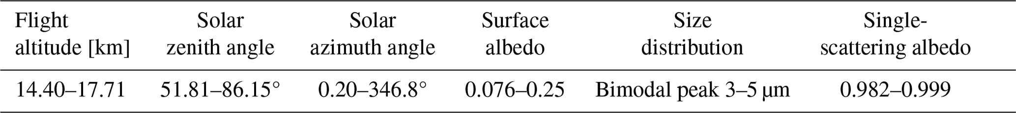
The model was set up in the same way as that described in Sect. 2.5. Cloud height and depth were determined from averages of the CPL data for this individual flight (due to operational constraints, this dataset was fairly sparse). The albedo was constrained by spectroradiometer observations. These observations are impacted by low clouds (not considered in the model) and thus surface albedo is likely biased high, although it is still in line with recent ice cloud RT modeling (Hong et al., 2016). The size distribution of ice particles used in the RT model was parameterized as bimodal with peaks at 3 and 5 µm; the single-scattering albedo of the ice particles was assumed to range from 0.982 to 0.999 in the 0.9–1.8 µm wavelength range. The choice of these parameters was constrained by preliminary simulation, in line with the findings of other studies (Rosenfield et al., 1998; de Reus et al., 2009). The average ice particle mass concentration was assumed to be the nominal value but was varied in different RT model runs in order to retrieve SIWP. It should be noted that, for a fixed size distribution and cloud geometry, SIWP and mass concentration are proportional. Based on Hawkeye observations of predominantly near-spherical particles, we use a Mie code to obtain the optical properties of the ice particles. Studies based on ATTREX data demonstrated how small particles increase with decreasing temperature (higher altitude) and how irregularly shaped particles are evenly distributed within the particle size distribution (Woods et al., 2018).

4.2 IWC retrievals

We performed SIWP model calculations for three different ice mass concentrations (nominal value IWC₀, IWC₀×0.5, and IWC₀×2), defining geometry and RT parameters for each observation (Fig. 8a). The modeled SIWP values bracket the observations and show the sensitivity of SIWP to ice water mass concentration. It is worth noting that the nominal ice mass concentration, associated with the average particle number density derived from the Hawkeye FCDP instrument, already leads to good general agreement with the observations (red line in Fig. 8a), with the exception of a notable mismatch between roughly 05:40 and 06:00 UTC. This difference is likely due to an actual ice mass concentration higher than the modeled value. The aircraft is descending at the beginning of this time interval, encountering more dense cirrus layers at lower altitudes that possess more than twice the averaged ice density assumed for the model. Another disagreement can be seen during the 07:26–07:40 UTC portion of the flight, where the model favors an ice density of about half of the nominal value. Overall, the comparison shows that observed SIWP and that calculated using the nominal ice mass concentration agree well for the remaining part of the observation time, with differences mostly of the order of <1 %–20 %. Panels (c) and (d) in Fig. 8 show the flight altitude and azimuth angle, respectively, showing the rapid ascent and descent of the aircraft as it spirals around the same atmospheric region. Despite the swift changes in geometry, simulated and observed SIWP consistently agree, revealing the efficacy of VLIDORT-QS to simulate SIWP observation at the limb for different geometries.

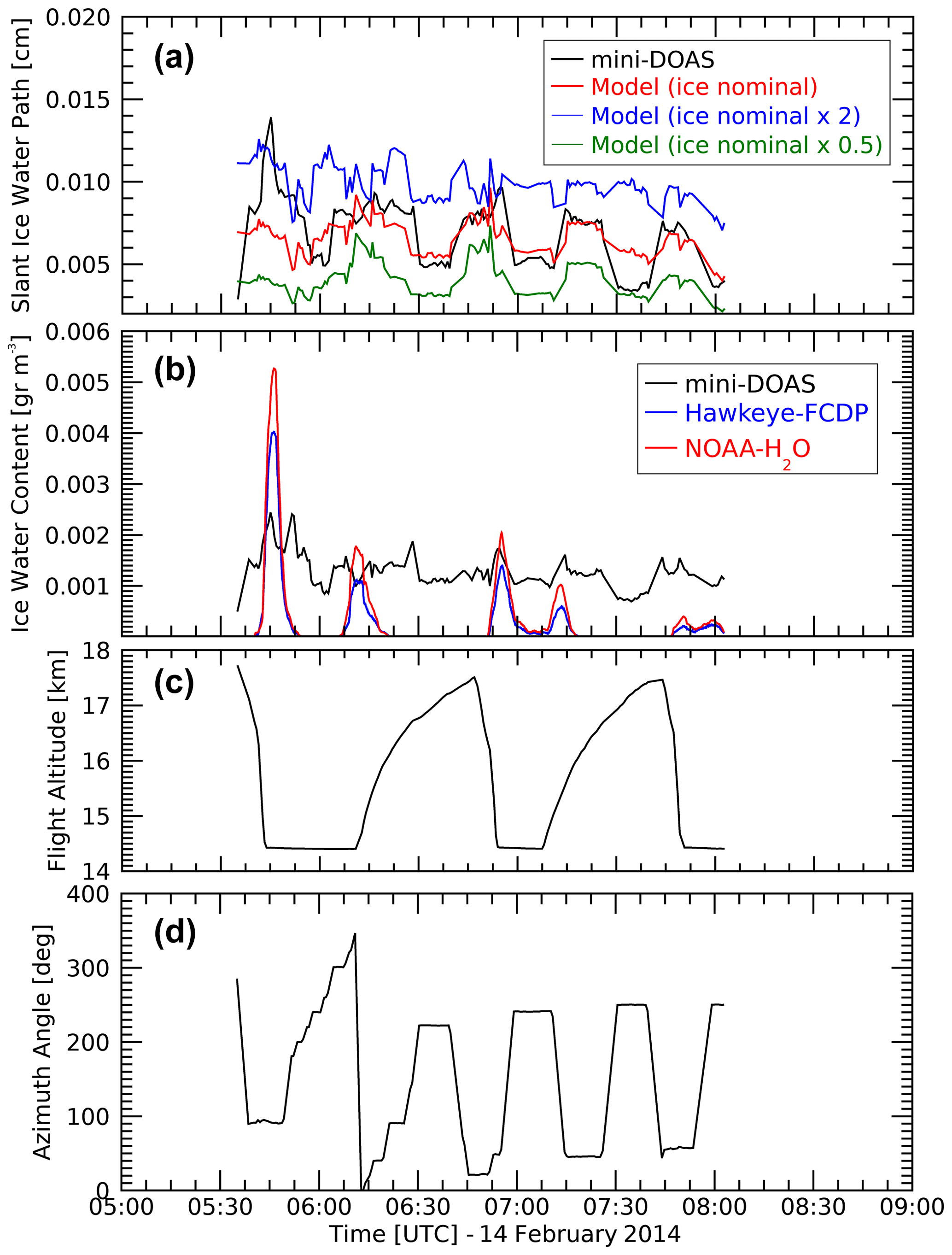
Figure 8 Comparison between the SIWP as measured by the mini-DOAS instrument and as simulated by the VLIDORT-QS model for three different ice number concentration values (a). Panel (b) shows the comparison of the ice water content (in g m⁻³) retrieved from the mini-DOAS observations and as measured by the Hawkeye FCDP and NOAA Water instruments for the portion of the flight considered. Flight altitude and azimuth angle are also shown (c and d, respectively).

Based on the knowledge gained from our sensitivity calculations, we then used a linear interpolation of the modeled SIWP to the observed SIWP in order to determine the IWC corresponding to the mini-DOAS measurements. The IWC for every observation is thus evaluated by scaling the nominal ice water content IWC₀ in order to achieve the best fit between the observed and modeled SIWP. The retrieved IWC varies between 0.001 and 0.0025 g m⁻³ and is independent of the variability imposed by RT effects on SIWP; these values are consistent with typical cirrus cloud ice water content levels observed in the TTL (Schiller et al., 2008; Thornberry et al., 2017). To better understand the ability of this methodology to detect thin cirrus cloud, an IWC detection limit was determined from the SIWP measurements. Time series IWCs are retrieved by interpolating the measured SIWP onto the modeled SIWP. Because a fit between the data points is used to invert SIWP to IWC, a standard IWC error can be calculated from the SIWP error and the propagation of the fit uncertainty.

Four different cases were chosen to represent the variability of the retrieved IWC from the measured SIWP. The four cases were chosen within the same flight, Science Flight 2, recorded between 16 and 17 February 2014 for the same geographical location (13° N, 144° E). The four cases had similar altitudes (16.6 km) but different solar zenith (57.5, 56.5, 25, 30.5°) and viewing azimuth (53.5, 138.9, 343.8, 138.4°) angles. IWC for these four cases ranges from 5.4 $\times {\mathrm{10}}^{-\mathrm{3}}$ to 0.02 g m⁻³, capturing a wide range of cirrus cloud conditions. The IWC error was determined by propagating the SIWP measurement error through the IWC retrieval for those four cases. A mean error of 1.39 $\times {\mathrm{10}}^{-\mathrm{4}}$ g m⁻³ was found. Defining the IWC detection limit as 3 times this mean error (∼ 99.7 %) leads to an average IWC detection limit of 4.17 $\times {\mathrm{10}}^{-\mathrm{4}}$ g m⁻³. It is worth noting that the NOAA instrument has an IWC detection limit of 2–$\mathrm{3}\times {\mathrm{10}}^{-\mathrm{6}}$ g m⁻³ for ideal conditions (Thornberry et al., 2015, 2017). While our IWC detection limit is not as good as that for the NOAA instrument detection limit, our approach is not affected by sampling artifacts (i.e., ice shattering), and it is sufficiently different and sensitive to provide new insights into cirrus clouds.

4.3 IWC validation

TTL cirrus cloud microphysical properties were widely sampled during the ATTREX 2014 campaign at altitudes ranging from 14 km up to the cold point tropopause (17.5–18 km), where temperatures were recorded in the 185–210 K range. In this region, cirrus clouds can extend vertically from 100 m to a few kilometers, with cloud temperatures decreasing with altitude following the lapse rate in the TTL. These observations resulted in the determination of cirrus cloud IWC from water vapor TDL measurements (NOAA Water instrument) and optical cloud probe (Hawkeye FCDP instrument) observations (Thornberry et al., 2017). The IWC retrieved from the observed mini-DOAS SIWP is then compared (Fig. 8b) to in situ measurements from these instruments for the same observational sequence. Due to spatial and temporal averaging of the mini-DOAS observations, a moving average of 4 min has been applied to the Hawkeye FCDP and NOAA Water data. This smooths some of the high IWC variability observed by these high-frequency in situ instruments.

For the portion of the flight considered here, lidar images from the CPL instrument showed consistent cirrus structures mostly between 15 and 16.5 km, with a mixed-cloud layer beneath (around 14–15 km). This can be clearly seen in Fig. 8b, where the Hawkeye FCDP and NOAA Water IWC values peak when the aircraft passes through the top and bottom of the cloud during ascending and descending flight stages (Fig. 8c). During the 15–16.5 km cloud transects around 06:15, 06:55, and 07:15 UTC, the in situ and mini-DOAS IWC data show good agreement in the core of the cloud. The comparison is less favorable for the measurements in the lower cloud deck, where the mini-DOAS is smaller (05:45 UTC) or larger (07:40 UTC). During the other periods, the mini-DOAS IWC is generally higher than that measured by the Hawkeye FCDP and NOAA Water instruments.

The IWC retrieved from the mini-DOAS observations seems to be more constant along the flight and less able to capture the small-scale variability of the ice. The reason for this difference is explained by the spatial averaging of the mini-DOAS instrument along the LOS. Due to the high altitude and limb-viewing geometry, observations are averaged over a very long path in the atmosphere that can reach up to 300 km ahead of the aircraft. The mini-DOAS will thus observe clouds even if the GH is flying in clear air that leads to near-zero or very low in situ Hawkeye FCDP and NOAA Water IWC.

It is well established that cirrus cloud microphysical properties are the result of a complex interaction of different parameters (Jensen et al., 2010) and that the variability in these parameters is the source of significant heterogeneity in the total IWC on both horizontal and vertical scales. This diversity can be measured by the change in IWC (or a related parameter) in the sampling step (at 1 s sampling rate, a high-frequency instrument such as the NOAA Water covers roughly 160 m horizontal distance and 35 m vertical for each data point). These in situ instruments are thus more sensitive to the local environment conditions at the time of acquisition, while the mini-DOAS gives a more averaged view of the presence of cirrus clouds.

Measurement comparisons between the different instruments therefore have to be interpreted with much care as the instruments probe different air masses. Nevertheless, the comparisons show that, considering these limitations, our retrieved IWCs from the mini-DOAS are comparable to those found inside cirrus clouds in the general observational area.

4.4 Retrieval uncertainty

In order to evaluate the uncertainties introduced by a change in the RT input parameters to the retrieved IWC for the flight segment considered, we performed sensitivity tests for different ice cloud heights and particle size distributions. We exclude situations where the aircraft was above the clouds, as limb observations of SIWP are less sensitive under these conditions. Limb observations are also challenging when the aircraft is in clear air below cirrus clouds, although retrievals are still possible. These overhead cloud situations can be observed more accurately by looking slightly upwards from the limb, something we did not explore in this study. Consequently, we do not consider retrieval uncertainties for these cases in this section. For the remaining cases, lidar data provided information on the altitude and the extent of the ice clouds for the portion of the flight considered, allowing the model to find the best fit between measured and modeled SIWP.

IWP can be obtained from the simulated SIWP, which provides IWC that is then integrated over the known cloud extension (definition of IWP). In order to get the IWPs and their uncertainties, we ran the RT model starting with the nominal case (assumed as the best retrieval), defined by a cloud deck from 14–18 km, and then modifying the extension of the cloud and the azimuth angle by fixed amounts. IWP uncertainty is then expressed as a percentage of the variation of the retrieved IWP from the nominal case for a variation of a specific parameter in the RT model (i.e., cloud height, SZA). To evaluate the uncertainties in the retrieved IWP we varied the geometrical extent of the cloud by three fixed quantities Δh (0.5, 1, and 2 km), subtracting Δh from the cloud top only, the cloud bottom only, and the cloud top and bottom simultaneously. As IWP is the IWC integrated over the vertical extent of the cloud, we discuss IWP uncertainties rather than IWC uncertainties. In addition, IWP is related more closely to the variation of the cloud extent, as modeled in this sensitivity test. This test revealed a significant dependence on the SAZ, making it difficult to assign a single value to IWP uncertainties imposed by a poorly known cloud height. We therefore report uncertainties, i.e., deviations from the base case, for the extreme values of SAZ for each case in Table 5.

When the vertical extent of the cloud in the retrieval is reduced by 12.5 % (Δh=0.5 km) from the top or bottom, IWP uncertainties are on the order of 5 %–10 % (Table 5). When the same quantity Δh is applied to both top and bottom (cloud is now reduced by 25 %), modeled IWPs differ from the best retrieval by 10 %–15 %. Uncertainties increase when a reduction of Δh=1 km is applied to the nominal cloud. In this case, a reduction of 25 % from the top yields 12 %–15 % uncertainty depending on azimuth, while a reduction of the cloud extent from the bottom produces 8 %–20 % uncertainties. When Δh is applied simultaneously to both top and bottom (cloud reduced by 50 % from the nominal value), IWP uncertainties roughly double to 20 %–35 %. For a further reduction of the cloud from the top (Δh=2 km, 50 % extent reduction), uncertainties increase to 30 %–40 %, while the same reduction from the bottom leads to uncertainties of the order of 20 % and 60 %.

Table 5 IWP uncertainties for three different cloud extent reductions Δh, for cloud top only, cloud bottom only, and both cloud top and bottom, as well as for different azimuth angles α.

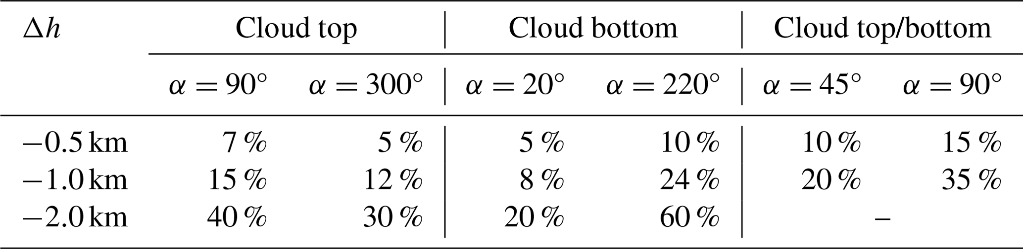
Overall, IWP uncertainties increase when the actual cloud geometrical extent differs from that for the nominal cloud used in the retrieval. This behavior appears to be relatively linear for a smaller cloud extent decrease (25 % the nominal height) for the top-only or bottom-only cases. When the reduction of the cloud height is more severe (50 %), the uncertainties of the modeled IWP become larger and depend more strongly on SAZ. It should be noted that, as IWP is the IWC integrated over the vertical extent of the cloud, the IWP uncertainties due to variations in cloud extent are solely due to the RT simulations. In order to reduce these uncertainties, additional methodologies, for example based on measured radiances or O₂ absorptions, are needed to constrain cloud extent when lidar data are unavailable.

The sensitivity of IWP retrievals to ice particle habit is beyond the scope of this study. However, we have evaluated the impact of uncertainty in the ice particle size distribution. The base IWP retrieval used a bimodal distribution with peaks at 3 and 5 µm. To test the influence of an uncertain size distribution, we increased the diameter of both peaks of the bimodal distribution by 1 µm and performed a retrieval of our data. The IWP changed by no more than 6 %, showing a low sensitivity to a change in the particle size and distribution. This result is encouraging, as obtaining particle size distributions for ice is difficult from remote sensing observations alone (Nakajima and King, 1990; McFarquhar and Heymsfield, 1997; Baran and Havemann, 2004).

5 Conclusions

This study explores the measurement of cirrus cloud ice water path using limb-viewing optical remote sensing of ice absorption in the near-infrared wavelength region. Our approach has not been reported previously in the literature, and this has required the development of new spectral retrieval methods as well as an enhanced RT model.

Spectral retrievals of the ATTREX mini-DOAS near-IR limb observations have clearly identified ice absorption in cirrus clouds through the retrieval of the slant ice water path, i.e., the integrated ice absorption along the complex photon paths through the atmosphere. In addition, O₂ and CO₂ absorption can successfully be retrieved in this wavelength region, providing additional information on the atmospheric RT.

We developed and applied a new extended version of the widely used VLIDORT model, called VLIDORT-QS (QuasiSpherical), which has the ability to simulate limb observations accurately. VLIDORT-QS is fully linearized and has the ability to generate simultaneous fields of Stokes four-vector and analytically derived Jacobians with respect to any atmospheric quantity, making it eminently suitable for forward-model simulations and sensitivity and retrieval studies.

Using these new tools, we performed a comprehensive sensitivity test of ice absorption in cirrus cloud for different parameterizations and subsequently developed a conceptual model of this measurement approach. This fundamental understanding of airborne near-IR limb observations is crucial for future efforts to explore this approach to study cirrus clouds from aircraft or satellites. Our conceptual model identified two general regimes:

1. a linear regime for thin and moderately thick clouds in which the ice absorption is proportional to the IWC and

2. a regime for thick cirrus clouds in which the ice absorption saturates and becomes independent of IWC.

Oxygen absorption does not contribute much information to the first regime but can be useful to study optical properties of ice particles in the second case. This was demonstrated in our paper but not further explored.

A feasibility retrieval of IWC from the limb mini-DOAS observations was also developed. This interpolation-based approach uses a small number of RT calculations for the viewing geometry of each observation to determine the sensitivity of SIWP to IWC. The retrieved IWCs also agree with those measured in situ by both the Hawkeye FCDP and NOAA Water instruments, although, due to the nature of its observation geometry, we found that the mini-DOAS IWC provides information on a much larger spatial scale and is thus less able to capture the high IWC variability inside cirrus clouds. Finally, this approach has shown the ability to detect IWC in limb geometry and its potential use as alternative method for the detection of cirrus at low ice water concentration.

Our study has demonstrated the value of near-IR absorption measurements to study cirrus clouds. As near-IR spectrometers are small and their technology is mature, our work points to a new way to measure cirrus cloud properties remotely.