An uncertainty methodology for solar occultation flux measurements: ammonia emissions from livestock production

Ammonia (NH₃) emissions can negatively affect ecosystems and human health, so they should be monitored and mitigated. This study presents methodology for the estimation of uncertainties in NH₃ emissions measurements using the solar occultation flux (SOF) method. The reactive nature of NH₃ makes its measurement challenging, but SOF offers a reliable open-path passive method which utilizes solar spectrum data, thereby avoiding gas adsorption within the instrument. To compute NH₃ gas fluxes, horizontal and vertical wind speed profiles, as well as plume height estimates and spatially resolved column measurements, are integrated. A unique aspect of this work is the first-time description of plume height estimations derived from ground and column NH₃ concentration measurements aimed at uncertainty reduction. Initial validation tests indicated measurement errors between −31 % and +14 % on average, which was slightly larger than the estimated expanded uncertainty ranging from ± 12 % to ± 17 %. Application of the methodology to assess emission rates from farms of various sizes showed uncertainties between ± 21 % and ± 37 %, generally influenced by systematic wind uncertainties and random errors. The method demonstrates the capacity to measure NH₃ emissions from both small (∼ 0.5–1 kg h⁻¹) and large (∼ 100 kg h⁻¹) sources in high-density farming areas. Generally, the SOF method provided an expanded uncertainty below 30 % in measuring NH₃ emissions from livestock production, which could be further improved by adhering to best application practices. This paper's findings offer the potential for broader applications, such as measuring NH₃ fluxes from fertilized fields and in the oil and gas sector. However, these applications would require further research to adapt and refine the methodologies for these specific contexts.

1 Introduction

Agriculture is the primary source of ammonia (NH₃) emissions, accounting for around 85 % of total discharges globally (EDGAR database, 2023) – a figure that has increased since pre-industrial times due to a growing food demand (Galloway et al., 2003). Among the different agricultural sources, livestock production releases NH₃ due to animal urine and faeces decomposition. NH₃ is a precursor of atmospheric fine particulate matter (PM_2.5) and eutrophication and an indirect greenhouse gas (GHG). PM_2.5 is associated with lung diseases, and NH₃ accounts for approximately 30 % and 50 % of PM_2.5 in the USA and in Europe, respectively (Wyer et al., 2022). The atmospheric lifetime of NH₃ ranges from hours to days, as it can either react in the atmosphere forming PM_2.5 or be retained in the ground due to dry or wet deposition. The complex emissions, reactions and deposition mechanisms of NH₃ hinder our understanding of these emission sources and associated dynamics (Hristov et al., 2011), so there is a need to monitor NH₃ emissions and atmospheric concentrations (Wyer et al., 2022). Knowledge gaps still need to be filled regarding NH₃ emission dynamics, which is reflected in the large discrepancies between modelled NH₃ and measured emissions (Lonsdale et al., 2017). A recent study on NH₃ emission hotspots using satellite data indicated that two-thirds of high-emission sources are underestimated by at least 1 order of magnitude (Van Damme et al., 2018). Furthermore, in Europe, NH₃ emissions are regulated under EU law (NEC 2016/2284) by reporting, monitoring and limiting emissions under certain thresholds (Wyer et al., 2022), which requires the development of emissions reduction technologies and reliable quantification techniques.

Consequently, NH₃ has gained attention over the last few decades, thus increasing the development of instruments and models used to study its emission sources. Moreover, with improvements in infrared lasers, spectroscopy-based instruments have emerged, such as FTIR (Fourier transform infrared) spectrometers, cavity ring-down spectrometers (CRDS) and quantum cascade laser absorption spectrometers (QCLAS) (Twigg et al., 2022). NH₃ concentrations are challenging to quantify due to their strong reactivity, which makes the gas molecule adhere to surfaces and requires that closed-path instruments and inlets are coated or heated to decrease the response delay (Zhu et al., 2015b). A study using 13 instruments highlighted the importance of the instruments' setup, inlet design and operation (flow rate and filter status), as these factors can affect measurement performance (Twigg et al., 2022).

Furthermore, measurements can be taken from mobile (Eilerman et al., 2016; Golston et al., 2020; Miller et al., 2015), stationary (Sun et al., 2015a) or airborne platforms (Guo et al., 2021; Miller et al., 2015; Sun et al., 2015b). Mobile platforms can resolve local scales very well (Golston et al., 2020), even though they are limited by road availability. Furthermore, Lassman et al. (2020) found that a surface-based platform can underestimate NH₃ emissions by a factor of 1.5 because concentrations near the surface might be depleted due to gas deposition. In addition, in recent years, satellite column retrievals have complemented information on NH₃ emissions from large-scale sources. These platforms have extensive spatial coverage but suffer from high-emission uncertainties and poor spatial and temporal resolution.

The solar occultation flux (SOF) has been used for years in the quantification of alkenes, volatile organic compounds (VOCs) and industrial NH₃ (Kille et al., 2017; Johansson et al., 2014; Mellqvist et al., 2007, 2010) and has been recently used to measure agricultural NH₃ emission sources (Kille et al., 2017; Vechi et al., 2023). SOF has been used in a mobile platform and in an aircraft (Kille et al., 2022). The SOF technique measures spatially distributed slant columns (g m⁻²), which can be converted to emission rates using additional information about wind speed and direction. The present paper is focused on the methodology and uncertainties of NH₃ measurements using SOF, while in the previously published Vechi et al. (2023) the attention is on the results from measurements using this methodology; therefore, they are supplementary to each other.

This approach can complement in situ and satellite measurements, effectively bridging these two techniques (Guo et al., 2021). The uncertainty with this technique has been briefly discussed before for VOCs (Johansson et al., 2013), alkenes (Mellqvist et al., 2010) and NH₃ (Kille et al., 2017). Herein, our aim is to further explore the error analysis with a comprehensive measurement uncertainty methodology and a comparison to validation experiments. Furthermore, we illustrate the use of the technique in three different case studies investigating NH₃ emissions from agricultural sources. Additionally, we provide the first description of plume height estimations obtained from the ground and column NH₃ concentration measurements. This study's results will also be valuable when using SOF for other species and in other applications. The novelty in the paper is threefold: (1) the plume height methodology, (2) validation of NH₃ measurements by SOF and (3) the uncertainty calculation following the guide to the expression of uncertainty in measurement (GUM) methodology.

2 Instrument, flux quantification and measurement campaigns

2.1 Instrumentation

2.1.1 SOF instrument and column retrieval

The SOF operation consists of recording solar infrared absorption spectra while driving below the gas plume (Fig. 1d and e). A solar tracker, which contains several mirrors, follows the Sun as the car moves and transmits solar light to the spectrometer where spectra are captured during sunny or low-cloud-coverage conditions. Further, for spectra measurements, an FTIR instrument (Bruker IR cube) is used with a resolution of 0.5 cm⁻¹ and a dual detector of InSb–MCT (indium antimonide, 2.5–5.5 µm; mercury cadmium telluride, 9–14 µm). The detection limit for NH₃ columns with the SOF instrument calculated as 3σ is 2.2 mg m⁻² at a sampling rate of 5 s.

Figure 1 (a) Example of spectra measured in the plume and in the background. (b) Measured and fitted absorbance spectra and the calculated residual spectra. (c) NH₃ calibration absorbance used to model the fitted spectra (approx. 40 mg m⁻³). (d) Example of solar spectral measurements when crossing the target plume. (e) Example of a box measurement around a target farm.

Alkanes are detected in the “C–H stretching band” at approximately 3.3 µm, while alkenes, propene and NH₃ are detected in the “fingerprint region” at around 10 µm. The specificity of NH₃ is strong because this species' absorption at the fingerprint region is unique, with sharp absorption features well-separated from other species (Fig. 1c). The retrieval of NH₃ was initially conducted in a narrow spectral window (940–970 cm⁻¹) and subsequently in a broader window (900–1000 cm⁻¹). The broader window results in a more stable retrieval of the atmospheric background, although with slightly increased spectral noise. The calculated enhanced column values represent the relative abundance compared to a reference spectrum recorded outside the plume (Fig. 1a). Ideally, a location as the representative of the external conditions should be chosen as the reference. In case of a noisy measurement, a posterior re-evaluation can be performed with a new reference spectrum. While retrieval of absolute columns is possible, which is done without decreasing the reference, the column results in a lower signal-to-noise ratio. The challenge with spectral retrieval is the long atmospheric path length of the solar spectra, which is affected by the strong absorptions of H₂O and CO₂ in the atmosphere; therefore, other interfering species are taken into account. Retrieval is performed by fitting a calibration spectrum from the HITRAN (Rothman et al., 2005) infrared database to simulate absorption spectra of the atmospheric background using a non-linear multivariate analysis and then calibrating according to pressure and temperature (Fig. 1b). The retrieval process is executed by custom software (Kihlman, 2005). For reference, the fitting procedure is described in more detail in Mellqvist et al. (2010).

Ideally, each SOF-measured transect should be recorded instantaneously, allowing the wind and turbulence conditions to be frozen in time. However, in practice, transects are carried out over a period ranging from a few seconds to minutes. This duration is influenced by the distance to the source, the size of the plume and the road characteristics, factors which inherently introduce uncertainties into the measurement.

2.1.2 Mobile extractive FTIR (MeFTIR) instrument

Before introducing the plume height calculation, it is necessary to present another measurement technique used for the quantification of plume heights in combination with the SOF columns. The mobile extractive FTIR (MeFTIR) was used to measure concentrations of NH₃ (mg m⁻³). The instrument consists of an optical multi-path cell connected to a heated, temperature-controlled FTIR instrument (Galle et al., 2001; Vechi et al., 2023). The measurements are made simultaneously with SOF. The MeFTIR was sampling from the car's roof, at about 2 m from the ground, while the SOF mirrors were also positioned at approximately the same distance to the ground.

2.2 Emission quantification using SOF

2.2.1 Emission calculation

The gas flux, also generally interpreted as the emission from the source, is initially derived by integrating measured column concentrations across the plume, following which the integrated mass of the target gas species can be obtained. To further calculate the flux, this integrated mass is multiplied by the wind speed parameter, u_t (m s⁻¹) Eq. (1).

$$\begin{array}{}\text{(1)}& \begin{array}{rl}{E}_{{\mathrm{NH}}_{\mathrm{3}}}& \left({\mathrm{mg}\mathrm{s}}^{-\mathrm{1}}\right)=u_t\left({\mathrm{m}\mathrm{s}}^{-\mathrm{1}}\right)\underset{P}{\int }{\mathrm{Column}}_{{{\mathrm{NH}}_{\mathrm{3}}}_l}\\ & \left({\mathrm{mg}\mathrm{m}}^{-\mathrm{2}}\right)\cdot \cos \left({\mathit{\theta }}_l\right)\cdot \sin \left({\mathit{\alpha }}_l\right)\mathrm{d}l\left(m\right),\end{array}\end{array}$$

where P is the transect path across the plume, l corresponds to the travel distance, and α is the angle between the wind and the driving direction. The slant angle of the Sun is compensated for by multiplying the concentration with the cosine factor of the solar zenith angle θ.

2.2.2 Determining the wind speed parameter

The wind is a vital part of SOF emission quantification (Eq. 1), and it should ideally correspond to the speed of the plume. However, wind speed measurements are not straightforward, as the wind is disturbed close to the ground and changes according to its height above the surface. Therefore, an approximation of the plume speed to be used as u_t is the average integrated wind profile (IWP_avg, Eq. 2) from ground to plume height (Fig. 2b). An assumption applied here is that the plume is vertically well mixed, meaning a similar concentration from ground to plume height, which is usually the case during sunny conditions. Additionally, in very unstable atmospheric conditions, the wind speed gradient is smoothed out by convection (Fig. 2a).

The IWP_avg is obtained using Eq. (2), where H_p is plume height (Sect. 2.2.3) and u_z is horizontal wind speed (m s⁻¹) measured at the different heights (z).

$$\begin{array}{}\text{(2)}& {\mathrm{IWP}}_{\mathrm{avg}}={\displaystyle \frac{{\int }_{\mathrm{0}}^{H_{\mathrm{p}}}{u}_z\cdot \mathrm{d}z}{H_{\mathrm{p}}}}\end{array}$$

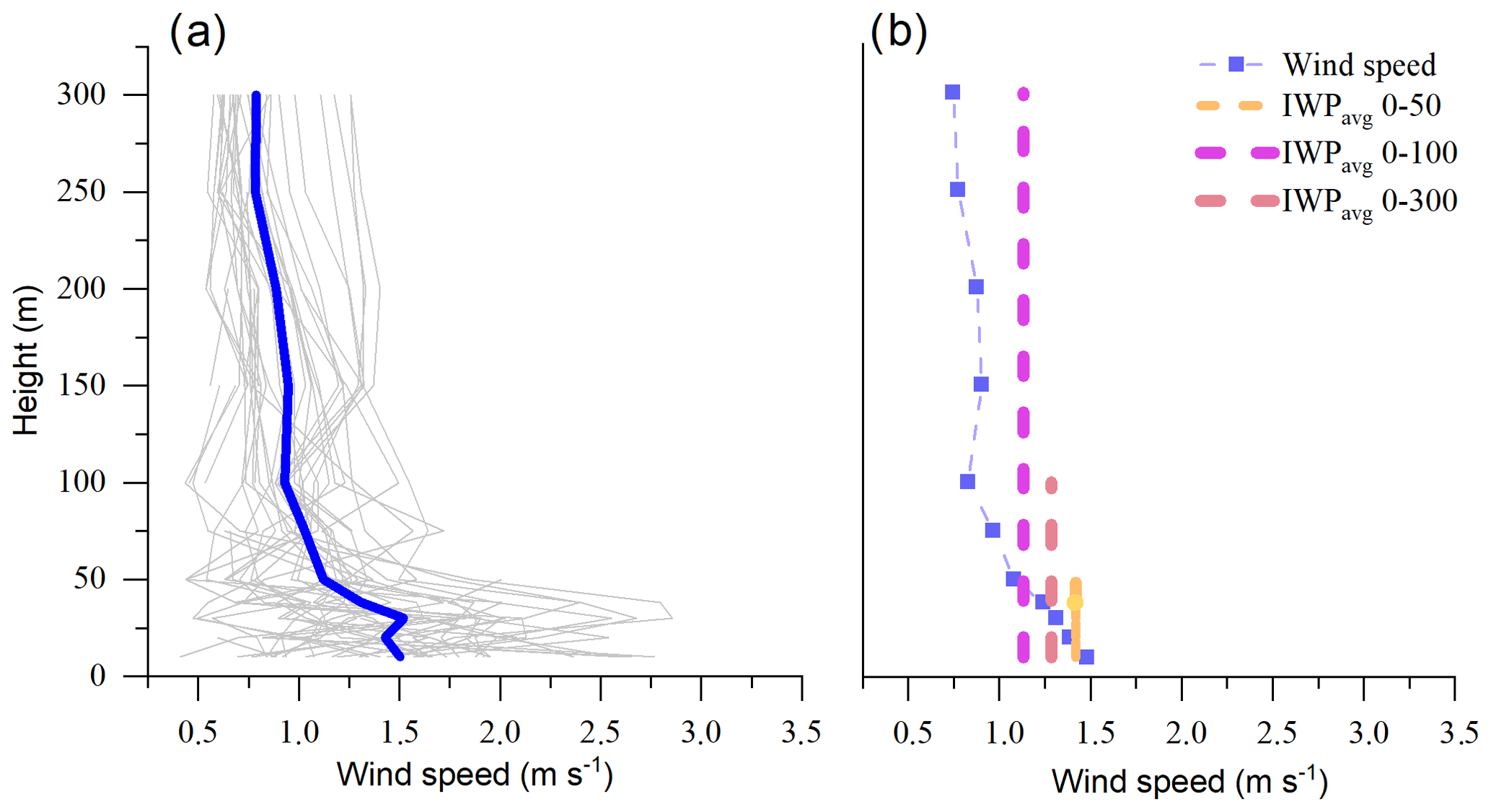
Figure 2 (a) Example of wind profiles; the grey lines show the individual profiles measured every 20 s and the blue line is the 10 min average. (b) An example of integrated wind profile (IWP_avg) at three different height intervals (0–50, 0–100 and 0–300 m) for a typical 5 min average wind profile.

2.2.3 Plume height (H_P)

To obtain the source's plume height, a novel approach is proposed which involves using the ratio between the vertical column (mg m⁻²) and the ground concentration (mg m⁻³) of NH₃ (Eq. 3). The results of this estimation are demonstrated in case study 3 (C3). This method relies on the assumption that the plume is well mixed vertically (Fig. 3, Case I). However, in reality, the plume might not disperse homogenously (Fig. 3, Case II or III), which brings uncertainty to the estimation, so it is considered an approximate assessment of H_p. For instance, when the plume is aloft (Fig. 3, Case II), this methodology produces an unrealistically large plume height in contrast to Case II, which is the opposite situation. Generally, solar insulation is strong during SOF measurements, which drives rapid vertical mixing and a plume dispersion like in Case I.

The NH₃ column (mg m⁻²) was obtained by the SOF method, while mobile extractive FTIR (MeFTIR) was used to measure ground NH₃ concentrations (mg m⁻³). In more detail, H^P is calculated by integrating the ground concentration and column while crossing the plume path l, where θ is the solar zenith angle (Eq. 3). This method is referred to herein as the vertical column ground concentration (VCGC) ratio. Furthermore, the H_p is calculated from the median of multiple transects.

$$\begin{array}{}\text{(3)}& H_{\mathrm{p}}={\displaystyle \frac{\int {\mathrm{Column}}_{{\mathrm{NH}}_{\mathrm{3}}}\left(l\right)\cdot \cos \left(\mathit{\theta }\right)\mathrm{d}l\left(\frac{\mathrm{mg}}{{\mathrm{m}}^{\mathrm{2}}}\right)}{\int \mathrm{Concentration}{}_{{\mathrm{NH}}_{\mathrm{3}}}\left(l\right)\mathrm{d}l\left(\frac{\mathrm{mg}}{{\mathrm{m}}^{\mathrm{3}}}\right)}}\end{array}$$

Alternatively, a rougher estimate of the H_P might be obtained from a simpler calculation (Eq. 4), considering horizontal wind speed (u_z) at the available height distance away from the emission source to the measurement road (P) and the speed at which the plume rises (σ_w) (m s⁻¹). Airborne measurements in Texas (Mellqvist et al., 2010) showed that the effective speed at which the plume rises from an industry in sunny conditions corresponded to 0.5 to 1 m s⁻¹, i.e. approximately the typical standard deviation of vertical wind (Tucker et al., 2009). Similar vertical wind data, i.e. ∼ 0.5 m s⁻¹, were measured using a lidar instrument in C3, referred to herein as “plume transport vertical speed” (PTVS).

$$\begin{array}{}\text{(4)}& H_{\mathrm{p}}={\displaystyle \frac{P\left(\mathrm{m}\right)}{u\left({\mathrm{m}\mathrm{s}}^{-\mathrm{1}}\right)}}{\mathit{\sigma }}_{\mathrm{w}}\left({\mathrm{m}\mathrm{s}}^{-\mathrm{1}}\right)\end{array}$$

Figure 3 An illustration of plume dispersion cases that can affect the plume height calculation. The y axis represents the plume height, while the x axis represents the volume mixing ratio (VMR). Case I: ideal scenario. Case II: H_p will be overestimated. Case III: H_p will be underestimated.

2.3 Campaign description

The SOF method was tested in a controlled release experiment and then demonstrated in three campaigns, each measuring NH₃ emissions from livestock production. The campaigns took place in France, the USA (California) and Denmark, namely countries with extensive agriculture production and significant differences in manure management and climate conditions. The campaigns were divided according to differences in wind measurements, the size of the target source and the interference of nearby sources.

2.3.1 SOF validation – controlled release test (Grignon, France)

A blind controlled release was performed over 3 d at a site in Grignon (France) to verify the accuracy of the SOF method for NH₃ emission quantification (Supplement, Fig. S1). Four release episodes were carried out by the French National Institute for Industrial Environment and Risks (Ineris) at release rates varying from 0.48 to 1.1 kg h⁻¹. Gas was released from a pure NH₃ cylinder (Air Liquide, 84 L, purity of > 99.99 %) equipped with a pressure regulator and a critical orifice (micrometric valve) to ensure a constant flow. The NH₃ cylinder was set on a high-precision scale (Mettler Toledo, range 1–100 kg, precision 2 g) to control the stability of the gas flow against time during the release. However, due to condensation and icing forming on the cylinder during release, the final release flow values were assessed by weighing the cylinder prior to and after release, which was done after the complete evaporation of the condensed moisture. Horizontal wind speed and direction were measured at 3 and 10 m in height using a vane wind monitor and the 2D sonic anemometer, respectively. Information on meteorological conditions such as temperature, relative humidity, precipitation and wind speed is shown in the Supplement (Fig. S2). The transect SOF measurements were conducted by FluxSense Inc. downwind of the release at average distances of 150–300 m. In order to ensure a proper blind test validation, release rates were unknown to the SOF operators until the final results were submitted.

2.3.2 Case study 1 (C1) – pig and dairy farm (Denmark)

Case study 1 consisted of a 2 d measurement campaign at two small-scale animal farms in Denmark, each of which was well-isolated from other interfering sources. NH₃ emissions were measured at a pig farm (C1a) and a cattle farm (C1b), and transects were performed at 250 and 900 m distances, respectively. The pig farm housed approximately 600 sows with piglets and weaners, while the cattle farm had approximately 700 dairy cows, plus heifers and calves. Horizontal wind speed and direction were obtained from two vane wind monitors placed on 3 m and 10 m high masts. Columns were measured downwind of the farms, while upwind fluxes were measured only once or twice because there were no other interfering sources.

2.3.3 Case study 2 (C2) – dairy complex (California, USA)

In case study 2, the SOF method was used to measure NH₃ emissions on a large dairy complex in Chino (California), a sizeable and concentrated area (21 km²) without other important NH₃ sources. Transects were collected in 1 d and were performed around the farm's fence line area, comprising a distance of 18 km for one transect. The area housed approximately 36 000 animals heads (CARB (California Air Resources Board), personal communication, 2015). One vane wind monitor performed wind measurements on a 10 m mast, and these were made by encircling the area; therefore, emissions were calculated by estimating the flux leaving the area minus the one entering it.

2.3.4 Case study 3 (C3) – dairy concentrated animal feeding operations (USA, California)

Lastly, case study 3 was conducted in dairy concentrated animal feeding operations (CAFOs) in the San Joaquin Valley (SJV), California. The results present the combination of the SOF (column) and the MeFTIR (ground concentration) instruments to demonstrate plume height calculations using the results from this case study. These were sources with large emissions, placed in high-farm-density areas. NH₃ measurements were made at the farms' fence line, approximately 1 km from the source, for 1 or 2 d for two farms (C3a, C3b). Upwind and downwind measurements were necessary to isolate emissions from the individual farm, due to other interfering sources near the target farms.

Wind measurements of the case studies

Wind measurements were generally recorded close to the source (∼ 100 m), except for C3, when a wind lidar was positioned approximately 5 km away. Most campaigns used a 2D sonic anemometer (WXT510, Vaisala) or a vane wind monitor (model 05103, Young) mounted on a 10 and/or 3 m mast. These 2D wind sensors quantified horizontal wind speed and direction. In the validation test, both anemometers were used (Vaisala and Young) at 3 and 10 m, respectively. In C1 two Young sensors were positioned at 3 and 10 m, while in C2 only one Young sensor was used at 10 m. In C3, a wind lidar was used, its detection principle based on the Doppler shift of an infrared pulse (∼ 1.5 µm) emitted by the instrument, which is then reflected by atmospheric aerosols. The instrument used in this campaign (Campbell Scientific, lidar ZX300) provided horizontal and vertical wind speeds and directions ranging from 10 to 300 m above ground at 11 different heights. In this case study, the IWP_avg was used as a wind parameter (u_t) for the emission calculations, averaging at 5 min and three height intervals, i.e. 0–50, 0–100 and 0–300 m.

3 SOF uncertainty methodology

This study establishes a methodology for quantifying the uncertainty associated with the solar occultation flux (SOF) measurements based on the guide to the expression of uncertainty in measurement (GUM) method (Joint Committee For Guides In Metrology, 2008). This shows for the first time the uncertainties in NH₃ SOF emissions measurements from livestock production based on the GUM (Joint Committee For Guides In Metrology, 2008) approach, and it also shows for the first time the methodology for plume height calculation, albeit drawing from principles outlined in the European measurement standard for VOC monitoring of refineries (CEN EN 17628 European standard, 2022). The investigation identifies and sums up both random and systematic uncertainties to establish a total standard 68 % confidence interval (CI 68 %) or expanded uncertainty (CI 95 %). It should be noted that most scientific articles, including past SOF studies (Johansson et al., 2013; Kille et al., 2017; Mellqvist et al., 2010), only consider standard uncertainties (CI 68 %). This paper, however, adopts a more comprehensive approach in line with industry and metrology institutes (Joint Committee For Guides In Metrology, 2008). As part of the uncertainty description, this study proposes a new method to assess spectroscopic uncertainties, demonstrating superior results with improved spectroscopic uncertainties when compared to the approach typically used in general spectroscopic measurements.

Emissions measurement random uncertainty is caused by many factors, with wind turbulence often being the most significant contributor. This uncertainty decreases in line with the number of samples taken; hence, the SOF European standard for refinery measurements recommends a minimum of 12–16 transects divided over several days (CEN EN 17628 European standard, 2022) for this type of source. In turn, systematic errors will persist independently of the number of transects. They are often correlated to the technique, instrumentation and measurement of other important variables, such as wind speed, and in this case, establishing best practices is one way to reduce them. The measurement uncertainty methodology is combined with data quality requirements which must be fulfilled for valid measurements. This includes sufficient solar height, relatively persistent wind direction and speed above 1.5 m s⁻¹, and sufficient measurement quality.

3.1 Spectroscopy uncertainty

Systematic spectroscopy errors can be divided into two categories, namely errors due to uncertainty in the strength of the absorption cross-section and imperfect spectroscopic fitting of the band shapes. An absorption strength uncertainty ($U_{\mathrm{abs}-{\mathrm{NH}}_{\mathrm{3}}})$ of 2 % (|(I_obs–I_cal)/I_obs|) for the NH₃ cross-section was found by Kleiner et al. (2003) for the full band of 700 to 1200 cm⁻¹. Therefore, it (U_cros) was calculated using absorption strength ($U_{\mathrm{abs}-{\mathrm{NH}}_{\mathrm{3}}})$ (Kleiner et al., 2003), further divided by 1.96, which is the coverage factor used for a 95 % confidence interval, as this error was considered a normal distribution (Eq. 5).

$$\begin{array}{}\text{(5)}& U_{\mathrm{cros}}={\displaystyle \frac{U_{\mathrm{abs}-{\mathrm{NH}}_{\mathrm{3}}}}{\mathrm{1.96}}}\end{array}$$

An imperfect spectroscopic fitting can have different causes, such as errors due to the shape of the reference cross-sections used, wavelength shifts or errors in instrument line shape characterization. Consequently, the spectroscopic fitting routine cannot account perfectly for all spectroscopic absorption features and may systematically overestimate or underestimate the column. The fitting residual, defined as the difference between measured and fitted absorbance, captures some information regarding the total fitting error. The root mean square (rms) of the residual is a commonly used measure of the fitting error magnitude, which can be used to estimate column uncertainty caused by fitting errors. Therefore, to assess the retrieval error (U_ret), we calculated the ratio between average NH₃ absorbance (abs) in 960 to 968 cm⁻¹ (abs_avg) (Fig. 1b) and the standard deviation (SD) of the fitting residual in the same wavelength range divided by the square root of the number of points (Eq. 6). The ratio was calculated for measurement points inside and outside the plume, and the linear regression curve's slope was considered to be the error.

$$\begin{array}{}\text{(6)}& U_{\mathrm{ret},\mathrm{1}}=\left({\displaystyle \frac{\frac{\mathrm{SD}}{\sqrt{n}}}{{\mathrm{abs}}_{\mathrm{avg}}}}\right)\end{array}$$

Previous studies (Griffith, 1996) have estimated the fitting uncertainty as

$$\begin{array}{}\text{(7)}& U_{\mathrm{ret},\mathrm{2}}={\displaystyle \frac{\mathrm{SD}}{{\stackrel{\mathrm{‾}}{\mathrm{abs}}}_{\mathrm{avg}}.}}\end{array}$$

Additionally, we estimated uncertainty based on dividing the integrated area under the fitting residual A_r with the integrated area under the fitted NH₃ absorption A_abs.

$$\begin{array}{}\text{(8)}& U_{\mathrm{ret},\mathrm{3}}={\displaystyle \frac{A_{\mathrm{r}}}{A_{\mathrm{abs}}}}\end{array}$$

In this study, different estimates were investigated by deliberately introducing errors into the fitted cross-sections and using these cross-sections in a spectral fit applied to a synthetic spectrum with absorption from a known column. Different uncertainty estimates (Eqs. 6, 7 and 8; Figs. S3, S4 and S5) were then calculated based on the residual from the fitting and compared to the error in the fitted column. The cross-sections included three error types: resolution error, shifting error and a multiplicative Gaussian noise error. For each case, a random error was chosen from each of the three types of errors within a specific range. The resolution error was a scaling factor in the range of 1 to 4, the wavelength shift error was an offset value in the range of −0.2 to 0.2 cm⁻¹ and the multiplicative Gaussian noise had a standard deviation from 0 to 0.1. In total, 1000 random simulations such as these were conducted, and Fig. 4a shows the resulting uncertainty estimates and column errors for each case. Figure 4b provides an example of the fitted NH₃ absorbance and residual for one of these cases. The uncertainty estimate in Eq. (7) was found to significantly overestimate the column error. In contrast, the uncertainty estimate in Eq. (6) was a better estimate, with the error being smaller than this estimate in roughly 95 % of cases. The uncertainty estimate based on the area (Eq. 8) was determined to significantly underestimate column errors in most cases.

Figure 4 (a) Column errors and systematic uncertainty estimates for 1000 simulated test cases. Uncertainty estimate from Eq. (6) in green, from Eq. (7) in blue and from Eq. (8) in orange. (b) Example of the fitted NH₃ absorbance for one of the simulated cases.

3.2 Background uncertainty

The background might differ in a systematic way on either side of the emission plume. Among other things, this might indicate the presence of a secondary source on the side or upwind of the target source (Fig. 5) or the influence of interfering background species when the solar angle changes. Background uncertainty (± U_B) corresponds to the relative difference in flux when choosing either the left or the right value as the assumed background. As the background value changes within the plume and is unknown, the uncertainty distribution is considered to be rectangular. Therefore, according to GUM (Joint Committee For Guides In Metrology, 2008), to obtain the standard uncertainty, it should be divided by the square root of 3 (Eq. 9).

$$\begin{array}{}\text{(9)}& U_{\mathrm{B}}={\displaystyle \frac{\frac{{\int }_{l\mathrm{1}}^{l\mathrm{2}}\mathrm{\Delta }{\mathrm{col}}_{\mathrm{Background}}\mathrm{d}l}{\mathrm{2}}}{\sqrt{\mathrm{3}}\cdot A_{\mathrm{col}}}}\end{array}$$

Here, Δ_col corresponds to the difference in the measured columns on either side of the allocated emission plume, which is integrated in the plume length (l) while A_col corresponds to the integrated column area across the plume.

3.3 Wind speed uncertainty

Wind speed is the largest source of uncertainty in SOF measurements (Johansson et al., 2013; Kille et al., 2017; Mellqvist et al., 2010). The wind speed parameter (u_t in Eq. 1) should be an approximation of the plume speed, in which case the IWP_avg is the best estimate of this parameter. Sunny, convective conditions smooth out wind gradient convection, which together with H_p estimation helps minimize errors. For the different case studies, the plume height was estimated according to the available information (Table 1), and only in case study 3 was the plume height measured (VCGC, Eq. 3).

In the validation test and C1, two wind masts held the wind monitors: one at 3 m and the other at 10 m. The wind profile was obtained by estimating the r factor using Eq. (10), where U is a known wind speed at two different heights. Thereafter, the obtained r factor was used to estimate the wind speed at the plume height (Eq. 11). Further, the IWP_avg was obtained using Eq. (2) by using the estimated wind profile. Furthermore, uncertainty was estimated by the difference between the measured wind speed (10 m), which was used for the flux calculations and the estimated IWP_avg from ground to H_p (Table 1, Eq. 12). For C2, only one 10 m mast was used to measure the wind, so we estimated the error of choosing different vertical profiles by using information from another study at the same geographic location and at a similar time of the year because of the lack of data to estimate the real wind profile. Moreover, in C3, we had a lidar as a wind sensor, so the IWP_avg was directly calculated at different height ranges (Eq. 2). Since the wind speed profile was actually measured instead of estimated, the error estimation in C3 is a better prediction of wind speed error (Table 1, Eq. 12).

$$\begin{array}{}\text{(10)}& {\displaystyle }r={\displaystyle \frac{\log (U_{\mathrm{2}}/U_{\mathrm{1}})}{\log (z_{\mathrm{2}}/z_{\mathrm{1}})}}\text{(11)}& {\displaystyle }{U}_{\left(z\right)}=U_{\mathrm{2}}{\left({\displaystyle \frac{z}{z_{\mathrm{2}}}}\right)}^r\text{(12)}& {\displaystyle }{U}_{\mathrm{wind}}={\displaystyle \frac{\left(\mathrm{1}-\frac{{\mathrm{IWP}}_{\mathrm{avg}}}{u_t}\right)}{\mathrm{1.96}}}\end{array}$$

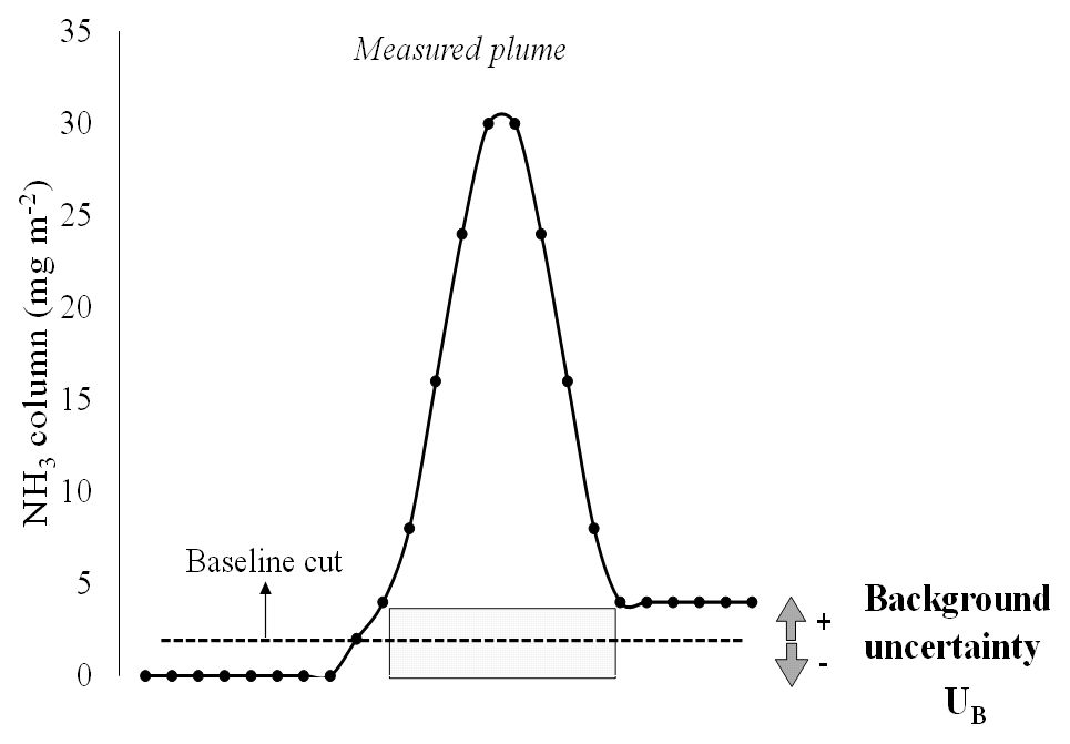
Figure 5 Assessment of systematic background uncertainty. The grey-shaded box represents the uncertainty area that might be added to the quantification. The calculation accounts for the difference between the background columns before and after the plume.

Table 1 Parameters used in calculating wind speed error uncertainty.

In this study, the uncertainty associated with wind direction was not factored into our measurements due to our knowledge of the source's precise location. This understanding allowed us to make necessary corrections to the wind direction, assuming that the emission plume moves uniformly from the known source. These corrections were based on visual observations made by the data processing operator. However, when the source location is not accurately known, it is crucial to consider and incorporate the uncertainty related to wind direction in the analysis. This approach aligns with the procedures followed in other SOF assessments when dealing with similar uncertainties (Johansson et al., 2014).

3.4 Calculation of standard and expanded total uncertainty

In each case study, random uncertainties, U_rand, were calculated as the standard error of the mean of the measured gas flux, as demonstrated by Eq. (13). The total variability is affected by the random variabilities of all the individual parameters that are used in the flux calculation according to Eq. (1). The overall random uncertainties decrease in an inverse proportion to the square root of n.

$$\begin{array}{}\text{(13)}& U_{\mathrm{rand}}={\displaystyle \frac{\left(\mathrm{SD}\right)}{\sqrt{n}}}\end{array}$$

For each case study, the systematic and random uncertainties were combined in a root sum square, resulting in the standard uncertainty (CI 68 %). Furthermore, by considering the methodology, the effective degrees of freedom were considered and expanded uncertainty (CI 95 %) was also calculated. Calculations followed the GUM methodology (Joint Committee For Guides In Metrology, 2008) using Eq. (14), where U_tot is the total relative uncertainty and k is the coverage factor (ranging from 1.96–3.00), depending on the degrees of freedom, N, and the confidence interval.

$$\begin{array}{}\text{(14)}& U_{\mathrm{tot}}=k\sqrt{\left(U_{\mathrm{cros}}^{\mathrm{2}}+U_{\mathrm{ret},\mathrm{1}}^{\mathrm{2}}+{U_{\mathrm{B}}}^{\mathrm{2}}+U_{\mathrm{wind}}^{\mathrm{2}}+U_{\mathrm{rand}}^{\mathrm{2}}\right)}\end{array}$$

4 Results

4.1 Uncertainty analysis

Each estimated uncertainty for the different case studies, as well as for the validation study, is shown in Table 2. Expanded uncertainty (CI 95 %) ranged from 15.1 % to 37.4 %, with a median value of 27 % for all case studies.

Here, the systematic wind uncertainty, U_wind, represents one of the largest sources of errors (Table 2) while wind turbulence contributes significantly to the random uncertainty. The estimated U_wind was particularly high in C1b and C2 because of the relatively high H_P (130–500 m), which was estimated by the PTVS method (Eq. 4), while wind information was obtained at 10 m high, thereby limiting the available field instrumentation. In contrast, in C3, despite the large H_P (400 m), wind speed measurements were made using a lidar, which gathers data up to a height of 300 m, resulting in an U_wind smaller than at C1b and C2. Additionally, in C3, the H_P was better estimated than in the other campaigns using the VCGC method (Eq. 3), which resulted in a decrease in U_wind and, consequently, total uncertainty. H_P is discussed in more detail in the following section. Moreover, for most case studies, several transects were recorded (>5); therefore, the random uncertainty, U_rand, was low. The exception was C2, which only had three transects, although these resulted in similar fluxes and therefore a low random uncertainty.

Table 2 Overview of estimated uncertainties for validation and in the other case studies. n/a: not applicable.

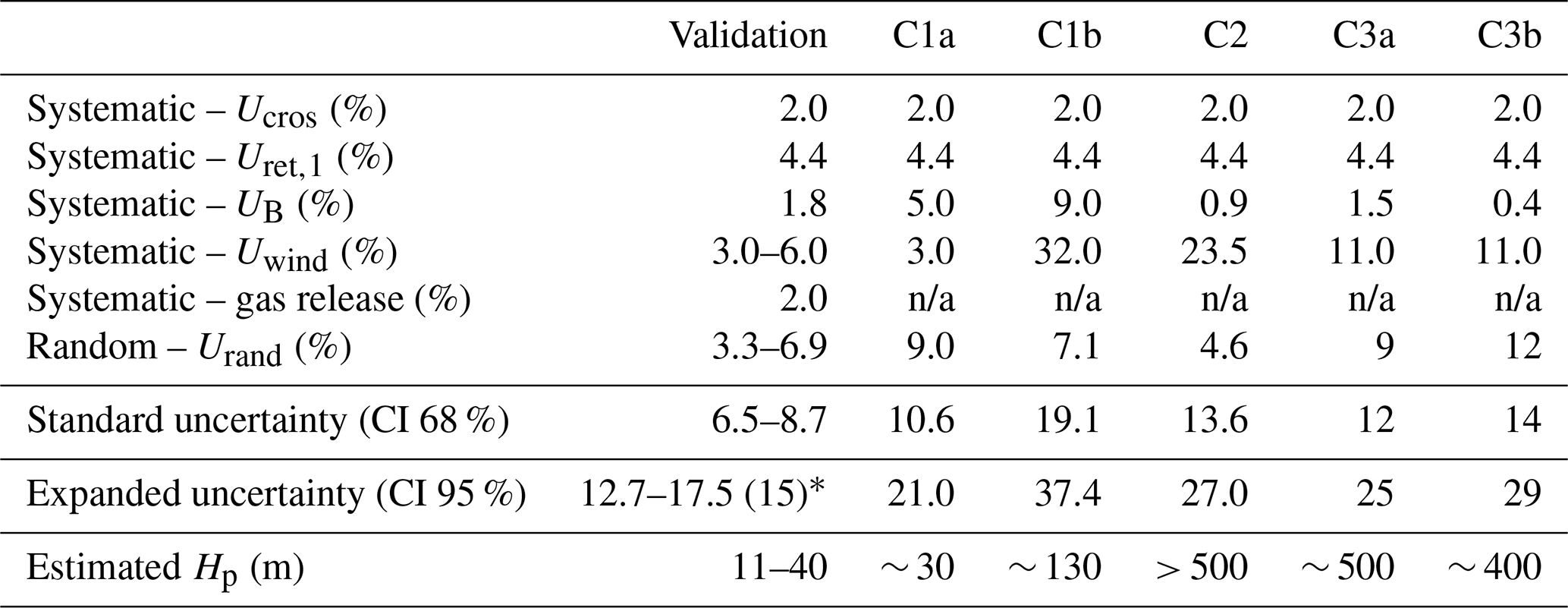
^∗ Average of the uncertainties found in the validation study.

Plume height (H_P) in case study 3

The MeFTIR and SOF were operated simultaneously in the vehicle, making it possible to estimate the plume height (H_p) using the VCGC method, according to Eq. (3), and to compare this to the H_p estimated using the PTVS method (Eq. 4). Figure 6a presents examples of NH₃ columns (left axis) and ground concentrations (right axis) measured in three distinct plumes (P1, P2 and P3). In the first peak, P1, the ground concentrations were comparable to P2 (right axis), while the column measurements were lower than P2 (left axis), indicating that P1 was located close to the ground. Conversely, P2 was at a higher height. Similarly, for P3, the columns (left axis) were lower than P2. However, the ground concentrations (right axis) were much higher, again suggesting a plume close to the ground (Fig. 6a). Furthermore, the second method (PTVS, Eq. 4) was utilized and compared to the VCGC method, showing that the first method produced, on average, emissions 35 % higher than the second where only one of the farms (farm 8) had a large difference (Fig. 6b). The VCGC method is more accurate as it does not require assumptions about the vertical plume speed. Additionally, in more complex cases, such as when the NH₃ source is spread and is heterogeneous (as seen in farm 8), the PTVS approach did not yield values similar to those in the VCGC method (Fig. 6b).

4.2 Validation

In the NH₃ validation test, controlled gas releases varied from 0.48 to 1.1 kg h⁻¹, while SOF NH₃ quantified emissions varied from 0.41 to 1.27 kg h⁻¹ (Fig. 7, Table 3). On average, wind speed varied from 3.8 to 5.9 m s⁻¹, and the direction changed from weak north-easterly winds on 22 September to stronger south-westerly winds on the two last measurement days. The weather conditions were sunny with low cloud coverage on 28 September and 1 October, while on 22 September the presence of clouds was more considerable, although measurements were still possible.

The relative error was between a minimum of −31 % and a maximum of +14 % (Table 3). Additionally, the calculated standard uncertainty (CI 68 %) ranged from 6.4 % to 8.7 %, and the CI 95 % ranged from 12.7 % to 17.5 % (Table 2). The estimated uncertainty explained the error observed only in the first release (Table 3, Fig. 7b), albeit within a 5 % difference in the last two releases (1 October). Potential sources of error include wind speed measurements, particularly as the estimated plume height ranged from 11 to 40 m (Table 3), while wind data were collected at 10 m in height. Although wind uncertainty was considered in the budget estimation, the lack of vertical wind profile measurements may have introduced limitations to the analysis.

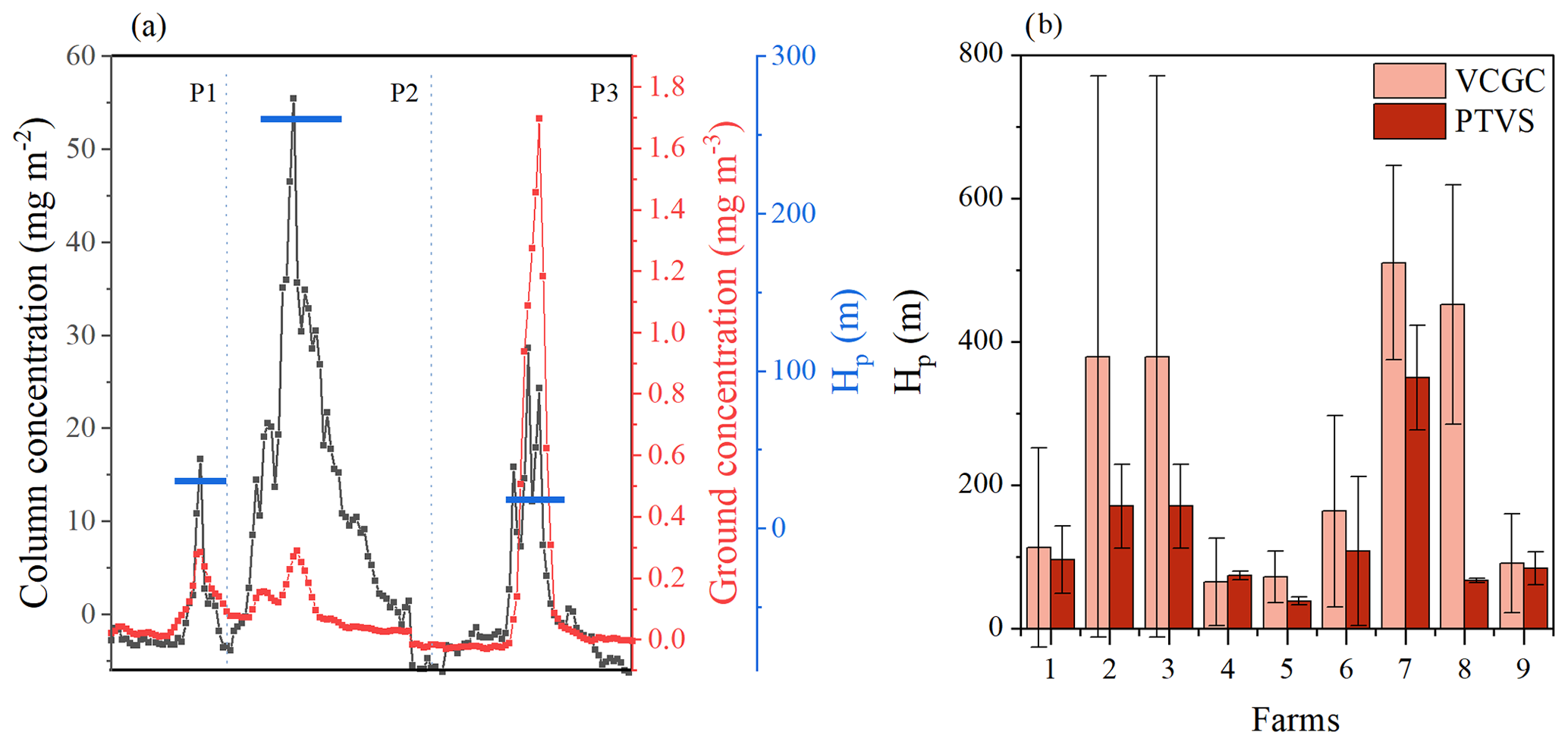
Figure 6 (a) Simultaneous measurements of NH₃ columns and ground concentrations. P1 and P3 were ground sources. (b) Examples of average plume height calculation from measurements at nine farms using the VCGC and PTVS methods. The light-red error bars correspond to the variation in the plume height estimation using the VCGC method, which is caused by variability in measurement distance and wind speed. The dark-red error bars correspond to the variation in the PTVS measurement data.

Figure 7 (a) Example of measured plume on 22 September at 14:55 (local time). The red dot indicates the NH₃ release point, and the arrow shows the wind direction. (b) Controlled-release rates and SOF-quantified rates (average ± expanded uncertainty (CI 95 %)). Map source: ©Google Earth.

Table 3 Overview of the NH₃ validation experiment.

^∗ Error estimated from 100 ⋅ (SOF emissions − controlled release) $/$ controlled release

In 75 % of the measurements, the NH₃ SOF quantifications were lower than the actual release, possibly due to NH₃ dry deposition or gas temporary loss in the release system, such as trapping in ice. NH₃ dry deposition depends on factors such as wind speed, source height, atmospheric stability, surface roughness length and surface concentrations (Asman, 1998). However, a deep analysis of NH₃ dry deposition is not part of this study as we focused on the methodology description. The measurements on 22 September exceeded the actual release, potentially impacted by less-than-ideal cloud conditions during the campaign, affecting the light intensity measured.

4.3 Case studies

These case studies were utilized to validate the solar occultation flux (SOF) method's effectiveness in measuring NH₃ emissions from various livestock production systems, in addition to assessing the real-world applicability of the developed uncertainty methodology. A measurement overview is provided in Table 4, and specific transect examples from each measurement campaign are depicted in Fig. 8. However, these emission data represent snapshots, confined to 1 or 2 d of measurement, and thus do not offer a reflection of annual emissions.

Table 4 Overview of results for the SOF NH₃ measurements.

^∗ Unknown numbers.

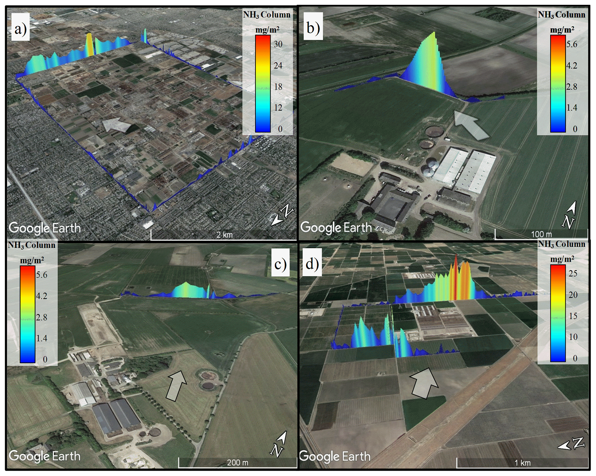
Figure 8 (a) (C2) NH₃ columns measured at Chino, made by encircling the feedlot area in a box; the arrow indicates the wind. (b) (C1a) Pig farm example (total farm), with the flux on the figure corresponding to 0.55 kg h⁻¹. (c) (C1b) Dairy farm plume example, with a corresponding flux of 2.52 kg h⁻¹. (d) (C3) Example of measurements from individual CAFOs. Upwind of the farm, there were emissions from the field. Map source: ©Google Earth.

4.3.1 C1 – small and isolated sources – pig and dairy single farms (Denmark)

Emissions from small and isolated farms are challenging to measure, primarily because of their low emissions and thus low concentrations, which are difficult to measure at a distance away from the farm. Total farm NH₃ emissions averaged 1.07 ± 0.23 kg h⁻¹ (CI 95 %) for pig farms (C1a, Fig. 8b). Thus, the SOF method could measure concentrations as low as 1 kg h⁻¹ with an uncertainty of ∼ 21 %. Emissions were normalized by livestock unit (1 LU = 500 kg of body weight) to obtain an emission factor (EF) of 2.4 ± 0.5 g LU⁻¹ h⁻¹, while the literature has reported EFs of 1.88 g LU⁻¹ h⁻¹ for the house only, not accounting for the manure tank (Rzeźnik and Mielcarek, 2016).

The dairy farm (C1b, Fig. 8c) had average emissions of 2.3 ± 0.9 kg h⁻¹, corresponding to an EF of 2.5 ± 0.9 g LU⁻¹ h⁻¹. Based on the literature, EF dairy farm houses are expected to have around 1.1 g LU⁻¹ h⁻¹ for the house only (Rzeźnik and Mielcarek, 2016). However, uncertainty in relation to wind speed measurements was relatively high (U_wind 32 %) due to limited wind instrumentation. Additionally, there is also the possibility of dry deposition due to the large distance between the source and the road used for the measuring equipment (800 m). Moreover, the emission rates obtained for C1a and C1b offer only a brief snapshot of daytime emissions, making comparisons with existing literature somewhat uncertain. This issue points to a larger uncertainty stemming from the inherent limitation of not capturing the full diurnal cycle. This factor can significantly impede effective comparison between different studies unless the data are normalized to a model predicting expected emissions across a full day–night cycle. It is important to note that this aspect relates more to the representativeness of the measurements rather than to any inherent issues with the measurement process itself.

4.3.2 C2 – box measurements of several sources – dairy complex (USA)

In case study 2 (Fig. 8a), the SOF method was utilized to quantify NH₃ emissions from the Chino dairy complex in California, USA. Although the emissions magnitude was significant, the extensive size of the complex (18 km perimeter) necessitated almost an hour to measure one box transect. This prolonged measurement time, coupled with potential changes in wind speed and direction, could have contributed to an increased uncertainty in the measurements.

NH₃ emissions averaged 245.0 ± 66 kg h⁻¹, while the EF was 6.8 g per head per hour. In comparison with the NH₃ flux estimations for this area using retrievals from a satellite (Infrared Atmospheric Sounding Interferometer, IASI; Van Damme et al., 2018), the emissions were similar to SOF at 4.3 g per head per hour (annual emission 2015) ranging from 1.1–51 g per head per hour. In contrast, other studies showed larger EFs ranging from 18.5 to 42 g per head per hour (October and June 2014; Leifer et al., 2017, 2018) and 14.9 to 79.7 g per head per hour (May and June 2010; Nowak et al., 2012). High fluctuations in NH₃ emissions are expected because they depend on meteorological factors (wind speed, temperature and solar radiation), although some variability might also result from the different techniques used. Here, the estimated measurement uncertainty was 27 %, with the U_wind being the largest source of errors.

4.3.3 C3 – large source surrounded by other sources – dairy CAFOs (USA)

One of the challenging types of facilities for the solar occultation flux (SOF) to measure is individual large-scale farms in areas of high farm density. The primary difficulty stems from interference from surrounding sources near the target farms. As such, upwind or box measurements, which encircle the source, were required to isolate the farm being measured (Fig. 8d).

Dairy CAFOs averaged 142 kg h⁻¹ for C3b and 165 kg h⁻¹ for C3a. The number of animals was not known; hence, emission factors (EFs) could not be established. Nevertheless, ammonia (NH₃) emission rates and EFs from these kinds of facilities have been documented elsewhere (Vechi et al., 2023). In Vechi et al. (2023), similar measurements of NH₃ by SOF were performed, and EFs were calculated according to the number of animals provided by the San Joaquin Valley Air Pollution Control District. Additionally, a diurnal pattern was observed, with emissions being highest around 12:00 LT.

In C3, the IWP_avg and H_p were measured differently from the other campaigns, i.e. estimated based on more uncertain calculations. Total expanded uncertainty ranged from 25 % to 29 %, and although U_wind was lower than the other campaign (11 %), random uncertainty made a large contribution (9 % to 12 %).

5 Conclusions and method application perspective

NH₃ emissions are challenging to quantify due to their high stickiness, which makes them difficult to sample without losses. Additionally, in the case of diffuse emissions from farms, NH₃ quantification might be hampered by an interference from fertilizer application and transport emissions or by dry deposition, meaning that concentrations are lost within a few metres of the source. These issues must be considered when designing and applying new instruments and methods. The SOF method has advantages for NH₃ quantification because it offers a contact-free measurement, thereby avoiding issues with gas adsorption into the gas inlet and instrument interior. Additionally, it has a fast time response (∼ 5 s) which, when combined with the flexibility provided by the mobile platform, helps cover large areas over a measurement day. Furthermore, the SOF method measures vertical columns, which is advantageous compared to ground concentrations as the latter might be affected by NH₃ deposition (Lassman et al., 2020). Moreover, SOF column measurements can be used to validate satellite column measurements, as has been recently done (Guo et al., 2021), and for CO measurements by SOF (Rowe et al., 2022). Estimating measurement uncertainty is essential because it indicates measurement precision; therefore, when comparing the obtained rates with other literature and models, uncertainty can better indicate whether or not values are significantly different.

Nonetheless, measurements using the SOF method are limited by required weather conditions, such as sunny skies and low cloud cover. As such, nighttime and heavily cloudy weather are not suitable for measurements. Additionally, the solar angle required for measurements leads to limitations for winter measurements at certain latitudes. NH₃ emissions are higher during daytime and sunny conditions, so, when using this method to estimate annual emissions or to compare to other studies and inventories, any diurnal emission variations must be considered (Lonsdale et al., 2017; Zhu et al., 2015a). This can be done by using models that estimate daily NH₃ variations by using meteorological information or other parallel measurements. Regarding NH₃ deposition, it will vary largely according to the conditions of each site. In California, for example, where both case studies 2 and 3 were performed, previous studies measured a deposition of 15 % in the first 3 km, while others estimated it to be from 8 %–15 % (Miller et al., 2015). For Denmark and France, these numbers might be higher because there was likely less convection during the measurement days; however, this paper focused more on describing SOF rather than investigating the emissions sources.

Here, the validation test and case studies have shown the SOF method's applicability and the accuracy level that the method can reach when best practices are followed. This study demonstrates that the wind speed vertical profile is a crucial parameter, which is more easily measured using wind lidar instruments. Additionally, to improve measurement accuracy and the choice of wind parameters, plume height should be estimated by combining measurements of ground and column. Furthermore, the technique was demonstrated to be suitable for large, concentrated areas and smaller sources with emissions as low as 1 kg h⁻¹, obtaining an uncertainty level ranging from 21 % to 37 % with a median value of 27 %. This study shows the potential of the SOF technique for a better quantification of diffuse NH₃ emissions related to livestock buildings, sources which are still poorly known.