the Creative Commons Attribution 4.0 License.
the Creative Commons Attribution 4.0 License.
 | 06 May 2024
U-Plume: automated algorithm for plume detection and source quantification by satellite point-source imagers
Jack H. Bruno
Dylan Jervis
Daniel J. Varon
Daniel J. Jacob
Current methods for detecting atmospheric plumes and inferring point-source rates from high-resolution satellite imagery are labor-intensive and not scalable with regard to the growing satellite dataset available for methane point sources. Here, we present a two-step algorithm called U-Plume for automated detection and quantification of point sources from satellite imagery. The first step delivers plume detection and delineation (masking) with a U-Net machine learning architecture for image segmentation. The second step quantifies the point-source rate from the masked plume using wind speed information and either a convolutional neural network (CNN) or a physics-based integrated mass enhancement (IME) method. The algorithm can process 62 images (each measuring 128 pixels × 128 pixels) per second on a single 2.6 GHz Intel Core i7-9750H CPU. We train the algorithm using large-eddy simulations of methane plumes superimposed on noisy and variable methane background scenes from the GHGSat-C1 satellite instrument. We introduce the concept of point-source observability, , as a single dimensionless number to predict plume detectability and source rate quantification error from an instrument as a function of source rate Q, wind speed U, instrument pixel size W, and instrument-dependent background noise ΔB. We show that Ops can powerfully diagnose the ability of an imaging instrument to observe point sources of a certain magnitude under given conditions. U-Plume successfully detects and masks plumes from sources as small as 100 kg h−1 in GHGSat-C1 images over surfaces with low background noise and successfully handles larger point sources over surfaces with substantial background noise. We find that the IME method for source quantification is unbiased over the full range of source rates, while the CNN method is biased towards the mean of its training range. The total error in source rate quantification is dominated by wind speed at low wind speeds and by the masking algorithm at high wind speeds. A wind speed of 2–4 m s−1 is optimal for detection and quantification of point sources from satellite data.
- Article
(1530 KB) - Full-text XML
- BibTeX
- EndNote


A number of satellite instruments can now detect and image methane column plumes with spatial resolutions finer than 60 m by observing solar backscatter in the shortwave-infrared (SWIR) range, enabling quantification of large point sources from individual facilities (Jacob et al., 2022). As the satellite observing system expands for both methane and other gases, there is a growing need for efficient methods of detecting and quantifying these point sources through automated processing of vast amounts of data. Here, we present the U-Plume algorithm, a generalized machine learning method, to address this need, and we apply it to methane observations from GHGSat (Jervis et al., 2021).
Several methods have been proposed for inferring point-source rates from satellite imagery of atmospheric pollution plumes, including those of methane (Varon et al., 2018), CO2 (Nassar et al., 2017), NO2 (Valin et al., 2013; De Foy et al., 2015; Beirle et al., 2021), CO (Pommier et al., 2013), SO2 (Fioletov et al., 2015; McLinden et al., 2016), and NH3 (Clarisse et al., 2019; Dammers et al., 2019; Noppen et al., 2023). Gaussian plume inversion (Bovensmann et al., 2010; Krings et al., 2011, 2013) and mass balance methods (Jacob et al., 2016; Buchwitz et al., 2017) have both shown success in estimating emissions for very large plumes (> 10 km), but they fail when applied to sub-kilometer plumes due to stochastic turbulence that leads to non-Gaussian behavior and dominance of eddy flow (Varon et al., 2018). Temporal averaging of plumes over multiple satellite passes with wind rotation has been used extensively for large plumes from well-identified point sources to decrease noise and enhance Gaussian behavior (Pommier et al., 2013; Fioletov et al., 2015; McLinden et al., 2016; Varon et al., 2020; Maasakkers et al., 2022); however, it is difficult to implement this approach for methane plumes, which are typically smaller and intermittent (Frankenberg et al., 2016; Cusworth et al., 2021; Irakulis-Loitxate et al., 2021; Ehret et al., 2022; Thorpe et al., 2023).
Two methods that have shown success in estimating emissions from high-resolution instantaneous-plume imagery are the integrated mass enhancement (IME) and cross-sectional flux (CSF) methods (Krings et al., 2011, 2013; Frankenberg et al., 2016; Varon et al., 2018). The IME method relates the total observed plume mass to a source rate, using information from the plume size and the local wind speed. The CSF method integrates concentrations over plume cross sections perpendicular to the wind direction and multiplies them by the local wind speed to infer a source rate. Both methods require the plume to be identified and masked (i.e., delineated) within the image.
Detection and masking of plumes in satellite scenes have generally been performed by human analysts (Guanter et al., 2021), but this is not practical operationally. Simple statistical thresholding approaches combined with adjacency criteria have been developed to detect methane enhancements above background for plume masking (Varon et al., 2019; Duren et al., 2019), but these are vulnerable to retrieval artifacts, particularly those from surface features mistakenly identified as methane plumes (Cusworth et al., 2019).
Machine learning presents a promising avenue for automating plume detection and inferring point-source emissions. Jongaramrungruang et al. (2022) proposed a convolutional neural network (CNN) to estimate source rates directly from aerial methane imagery obtained from the Airborne Visible InfraRed Imaging Spectrometer – Next Generation (AVIRIS-NG). Their method (called MethaNet) provides source rate estimates based solely on methane column retrieval fields, forgoing the use of external information on wind speed by exploiting wind information contained in the morphology of the plumes (Jongaramrungruang et al., 2019). Training and testing of MethaNet have been done on aircraft imagery with a relatively clean background and high pixel resolution (3 m), but to our knowledge, it has not been applied to satellite imagery which is coarser and more vulnerable to surface artifacts. MethaNet does not produce a plume mask (outline of plume boundaries), but such a mask offers important visual information and can help identify artifacts. Joyce et al. (2023) used a U-Net architecture to mask methane plumes in PRecursore IperSpettrale della Missione Applicativa (PRISMA) satellite imagery directly from radiances, again without incorporating wind speed information. Separate networks were then used for inferring methane column concentration and estimating emission rates. In both MethaNet and the Joyce et al. (2023) approach, there is a bias towards the training mean in the final source rate estimates, resulting in an overestimate of low-emitting plumes and an underestimate of high-emitting plumes. This is a common issue in machine learning applications.
Here, we perform binary segmentation of methane column imagery from GHGSat using a U-Net neural network architecture to produce plume masks, and we then use these masks, together with wind speed information, to infer point-source rates either with a CNN or with the physics-based IME method. We use wind speed information because some is always available – either from local measurements or from regional/global reanalysis datasets. The U-Net architecture (Ronneberger et al., 2015) has previously demonstrated its effectiveness in feature recognition by means of binary image segmentation from satellite imagery (Joyce et al., 2023), avoiding the false positives present in more traditional methods reliant on thresholding (Rezvanbehbahani et al., 2020). Combining the U-Net architecture for detecting plumes in column enhancement with subsequent steps for inferring point-source rates forms an end-to-end algorithm that we call U-Plume.
We present here the U-Plume algorithm for identifying point-source plumes in satellite imagery of methane concentrations and inferring point-source rates. The algorithm has two components: (1) a U-Net for detecting plumes by means of binary segmentation of the pixels in the satellite scene (0 denotes background; 1 denotes plume), producing a plume mask, and (2) two alternative CNN and IME approaches for inferring source rates from the plume mask. We demonstrate U-Plume using the GHGSat-C1 instrument for methane, but the architecture and training process presented here are potentially applicable to any satellite point-source imagers for any species.
GHGSat-C1, launched in 2020, is the first operational instrument released by GHGSat Inc., since the demonstration instrument GHGSat-D was launched in 2016 (Jervis et al., 2021). The instrument is a shortwave-infrared interferometer with an observation domain of at a 25×25 m2 pixel resolution. Retrieval of the backscattered solar spectrum at the 1.65 µm methane absorption band yields an estimated methane column mass enhancement over background that is reported in terms of mol m−2 with 1 %–2 % estimated precision. The instrument is in a polar sun-synchronous orbit, with observations conducted at ∼ 09:30 LT. Subsequently launched GHGSat-C2-C11 instruments have less background noise than GHGSat-C1. Our results can be extended to GHGSat-C2-C11 and any other instruments using the background noise metrics presented below.
Our first step is to create a training dataset of plume-containing satellite images in which synthetic instantaneous plumes with known source rates are superimposed on actual plume-free images. Following Varon et al. (2018) and Jongaramrungruang et al. (2019), we use the Weather Research and Forecasting model large-eddy simulations (WRF-LES) to create a diverse plume dataset of atmospheric methane concentration enhancements, where the relationship between source rate and plume concentration is known. Point-source methane emission and atmospheric transport are simulated on a 25×25 m2 horizontal and 15 m vertical grid over a domain, with the point source emitting at the surface five-sixths of the way from the downwind edge of the domain. We conduct four simulations for different meteorological conditions, each of which is run for 3 h with the first hour used as spin-up, resulting in 2 h of usable plume images per simulation. Time steps for WRF-LES integration are set at 0.25 s, and instantaneous plumes are sampled every 30 s. Mean wind speeds for the simulations are between 3–9 m s−1, with sensible heat fluxes of 100–300 W m−2 and mixed-layer depths of 500–2000 m. This is the same ensemble as that used by Varon et al. (2021), where the specific details of the simulations are provided.
To create an effective neural network, the training imagery must be as close as possible to the real observations that the model will be applied to. In previous work by Varon et al. (2018) in which the WRF-LES was used to simulate synthetic plumes, these plumes were superimposed on a white-noise background to generate a training dataset; however, variable surface albedo and terrain can lead to heterogeneous noise fields with complex structures. To create realistic noise for our training images, we start with a set of actual GHGSat-C1 observations of plume-free scenes and add the methane column enhancements from the WRF-LES. We use the standard deviation of the pixel enhancements in the plume-free scene (ΔB, kg m−2) as a measure of background noise:
Here, n is the number of pixels in the image, xi is the column concentration for the individual pixel i, and is the mean column concentration in the scene. When discussing ΔB, we express it as a percentage of the global mean background concentrations (taken as xb=0.011 kg m−2; Jervis et al., 2021). We use 28 plume-free GHGSat-C1 observations (each measuring 12 km × 12 km) corresponding to a variety of surface types. Scenes with ΔB < 5 % correspond to homogeneous bright surfaces, including arid and grassland terrain. Scenes with 5 % < ΔB < 10 % correspond to moderately heterogeneous surfaces. Scenes with ΔB > 10 % correspond to very heterogeneous or dark surfaces, including forests, wetlands, and urban areas. Values of ΔB are instrument-dependent. The more recent GHGSat-C2 and subsequent instruments have ΔB < 2 % under most observing conditions (Ramier, 2023). On the other hand, hyperspectral/multispectral land surface mappers can have background noise exceeding 10 % (Cusworth et al., 2019; Varon et al., 2021).
Figure 1 illustrates the steps for creating the synthetic plume observations used in training and testing our method. For each training image, a 128-pixel × 128-pixel scene is randomly selected from a plume-free GHGSat-C1 observation. A random plume from the WRF-LES dataset is then selected, with a random rotation and translation applied to situate the plume anywhere in the scene but with a safeguard to ensure that the plume is fully contained in the scene. Since the methane enhancement in the plume is proportional to the source rate, we can scale the plume randomly to correspond to a given source rate. This plume image is then added to the selected scene to create a training image. A training range of plumes emitting in the 500–2000 kg h−1 range is chosen to ensure that the plumes are at least partially visible in most training images. Though we want the network to be able to detect smaller source rates, it is important that the structural features being searched for are visible above the noise within the training dataset. Because the U-Net recognizes structure (and not just enhancement), the network trained using the 500–2000 kg h−1 range is still usable outside of this range, as we will see. Because pixel values for methane enhancement generally fall into the −0.3 to 0.3 mol m−2 range, we found that it is not necessary to normalize the data for training.

Figure 1Sample generation of U-Plume training imagery. The first panel shows a plume-free observation sample of methane column concentration enhancements observed by GHGSat-C1. The second panel is a 128-pixel × 128-pixel scene randomly selected from the full observation domain. The third panel shows a WRF-LES instantaneous-plume sample for a source rate of 2000 kg h−1 – we chose a large plume here for easy visualization. The fourth panel shows the result of adding the second and third panels to form a training image. A total of 0.1 mol m−2 corresponds to a dry column mixing ratio enhancement of 284 ppb.
Our set of training and test images is created using 28 plume-free observations. We step the 128-pixel × 128-pixel scene over each full image in 16-pixel steps to create a set of scenes. The ΔB values of these scenes range from 1 % to more than 50 %. We only use scenes with ΔB < 20 % to avoid training in scenes with extremely high background variability, where the detection of any but the largest plumes would be intractable. This filtering leaves us with a total of 6870 scenes, with a median ΔB of 8 % and interquartiles of 5 % and 12 %. We then apply the random plume placement and source magnitude as described above to create 6870 simulated-plume observations. This is a relatively small set for training by machine learning standards, but it is sufficient for providing a successful network which could be easily bolstered by a future collection of additional large-eddy simulations (LESs) and background images. The true plume mask is composed of pixels where the enhancement from the LES is higher than the ΔB of the scene, which is the criterion for the pixel contributing more information than the noise (Varon et al., 2018). Moreover, 90 % of the images are used for training, and 10 % are set aside for testing. We use a relatively standard configuration of the U-Net model with a modest training period and therefore do not have a separate validation set for specific learning-rate stopping criteria. The metric we use to measure masking success is the Jaccard score, which is derived from the intersection of the predicted mask (A) and true mask (B) over the unity of the two:
We train the model for 20 epochs with a batch size of 32 images, minimizing a loss function (L) that combines binary cross-entropy (BCE; Jadon, 2020) and the Jaccard score. This loss function is defined as
Figure 2 shows the two-step process used to obtain source rate estimates from methane enhancement images. First, a U-Net masking network is used to identify pixels in which a plume is present. The binary mask created by this network is then fed along with the original enhancement image and external wind speed data to estimate the source rate from the identified plume. The enhancement image with the mask is preserved for visualization and as a quality control diagnostic. Processing the test dataset of 687 images, preloaded from their relevant files, in 32 image batches on a single 2.6 GHz Intel Core i7-9750H CPU takes 11 s, corresponding to 62 images per second.

Figure 2U-Plume architecture. Starting from a methane enhancement image (the sample image in Fig. 1), we use the U-Net machine learning algorithm to produce a plume mask (in red) of pixels containing more information than noise. All masked pixels in a single 128-pixel × 128-pixel (3.2×3.2 km2) scene are assumed to originate from the same plume. We then use the original enhancement image, the mask, and local 10 m wind speed to quantify emissions using either a machine learning method or an integrated mass enhancement (IME) method.
The U-Net neural network for plume masking (Ronneberger et al., 2015) uses an encoder–decoder framework to recognize structural features within imagery. The network receives a methane enhancement image, such as that in Fig. 2, and classifies each pixel with a confidence level for the presence of a plume. We apply a threshold of 50 % confidence to produce a binary plume mask. The main advantage of this method over traditional threshold masking is that high-enhancement features that do not have plume-like shape characteristics will not be falsely captured as plumes.
The encoder portion of the network applies a series of convolutional filters and pooling layers to identify features of increasing complexity within the image. By the end of the encoding process, the image will have been compressed spatially and have many channels corresponding to the various feature maps created by the convolutional filtering. By compressing the image spatially in this way, the network can recognize connections between distant features.
The decoder portion of the network serves to interpret these identified features as criteria for classification. An inverse convolutional operator is used to expand the spatially compressed image back to the original size of the input image while reducing the number of filters applied, which compresses the number of channels in the image. The final step of the network uses the information gathered from the encoder–decoder process to estimate a confidence level (0–1) for each pixel that determines whether it is or is not part of a plume. Output from this model for a single image is a confidence mask for plume location across the enhancement image, as shown in Fig. 2. In practice, the confidence mask is generally either very close to 1 or very close to 0. Intermediate values fall off very quickly at the edge of the mask. We deviate from the Ronneberger et al. structure only in that we begin with 16 convolutional filters rather than 64 and thus reach a maximum channel depth of 256 rather than 1024 at the end of the encoder path. A loss function combining binary cross-entropy and the Jaccard score is minimized for the training set. The code used for the model creation and loss function can be found alongside our dataset in the repository at the end of this text (https://doi.org/10.7910/DVN/YFRQU4, Bruno, 2023).
Once the U-Net mask has been generated in the first step of our U-Plume algorithm, we infer the source rate in the second step, using either a CNN method or an IME method. The CNN method utilizes a three-channel input image containing the original image, the binary mask, and 10 m wind speed. Initial testing indicated that including wind direction did not improve performance. The wind speed channel is populated with a uniform (15 min scene) average value from the LES. The CNN uses a series of convolutional and pooling layers which connect to a set of fully connected layers, rather than a decoder, to yield a scalar estimate of emissions. The CNN structure is identical to that of the U-Net truncated at the end of the encoder path and is connected to 32-node and then 16-node dense layers with a single-node output layer. All three of the added layers use a rectified linear unit (ReLU) activation function, and the model is trained using a mean squared error loss. We train the model for 10 epochs with a batch size of 32 images and use U-Net-generated masks for the mask input channel (limited to successfully masked examples). Optimization of this structure and training process could potentially improve the results of the CNN.
The IME method follows Varon et al. (2018), in which the plume mass enhancement (IME) is combined with a parameterized effective wind speed (Ueff) and plume length scale (L) to infer the source rate (Q, kg h−1), which is defined as
The plume length scale L is defined as the square root of the plume mask area. The effective wind speed is fitted to the 15 min averaged wind speed U10 at 10 m altitude using the training dataset, where the relationship between Q, IME, and L is known for a given U10. This yields
with Ueff and U10 given in units of m s−1. The intercept of 0.7 m s−1 arising from the fit can be physically interpreted as a minimum turbulent diffusion for the plume at low wind speeds. This calibration is specific to the GHGSat-C1 instrument and should be recalculated when applying U-Plume to other platforms.
We introduce the concept of point-source observability (Ops) as a dimensionless number to determine the ability of a satellite instrument to detect and quantify point sources. Observability is a function of source rate (Q, kg s−1); wind speed (U, m s−1); instrument pixel resolution (W, m), which is 25 m in our case; and scene-dependent background noise (ΔB, kg m−2 – as defined in Eq. 1).
The idea behind the Ops concept is that the observability of point sources is determined by the signal-to-noise ratio in the plume (Varon et al., 2018). The column concentration enhancement in the plume (kg m−2) scales as (Jacob et al., 2016). The noise for a given scene (kg m−2) is given by ΔB, which is a scene-dependent property of the instrument that can be characterized as a function of the surface type. ΔB can be viewed as the precision of the instrument accounting for the contribution from surface artifacts. The dimensionless point-source-observability number Ops is then given by
and is a measure of the signal-to-noise ratio. We will use it here to interpret our results, but it can be applied more generally to any remote sensing observation of point sources.
4.1 Plume detection and masking
Figure 3 shows the relationship between source rate and U-Net masking success. In 2 % of cases, no mask is produced for the image, and in 30 % of cases, there is no overlap between the true and predicted masks. These failures occur for high background noise (ΔB > 5 %) and lower emission rates. On the other hand, Jaccard scores generally exceed 0.5 for low background noise (ΔB < 5 %).
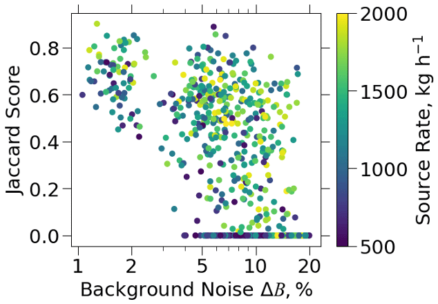
Figure 3Ability of the U-Net machine learning algorithm to delineate (mask) plumes emitted from point sources. Masking success is measured using the Jaccard score (Eq. 2) and is plotted as a function of background noise ΔB (Eq. 1) for a range of point-source rates from 500 to 2000 kg h−1. Results are for the test set of WRF-LES plume images superimposed on noisy plume-free observations from the GHGSat-C1 satellite instrument.
We examine false positives by applying the network across the test dataset of backgrounds without plumes added. This yields masks in 14 % of cases (false-positive detection rate). The masks produced in these false positives are generally very small, with a median size of 5 pixels. Applying a minimum mask size of 5 pixels brings the false-positive rate down to 6 % while losing only 1.6 % of the true-positive detections in the test dataset and removing 92 % of the zero-overlap masks. False positives occur most commonly in scenes with high ΔB values and particularly in scenes with complex topography. The mask sizes for these false positives are generally small, as evidenced by the effectiveness of the mask size filtering, and their corresponding estimated source rates are therefore also generally small.
In Eq. (6), point-source observability (Ops) provides a dimensionless scaling number to better understand how point-source detection for a given instrument relates to the combination of source rate, background noise, wind speed, and pixel size. Here, we use 10 m wind speed (U10) for the calculation of Ops. We create an augmented test dataset with 10 subset images from each of the 28 plume-free observations (Fig. 1) and 20 emission levels, ranging from 100 to 2000 kg h−1 in 100 kg h−1 increments, for each image. We bin images in the augmented test dataset based on their Ops, ranging from 0.005 to 0.5 in 201 log-spaced bins. Additionally, for each bin with a minimum of 50 images, we calculate the probability of detection as the fraction of plumes in the bin with J > 0.1. Figure 4 shows the relationship between the probability of detection P and Ops. The relationship when Ops > 0.014 can be tightly fit to a sigmoid function of the following form:
Detection probability is 10 % when Ops=0.02, 50 % when Ops=0.04, and 90 % when Ops=0.08. The transition from low detectability (< 10 %) to high detectability (> 90 %) is very sharp in Ops space, demonstrating the power of the Ops metric in evaluating the ability of plume-imaging instruments to observe point sources. The Ops value of 0.04 at the 50 % detection threshold can be interpreted as a characteristic column-averaged concentration enhancement, , in the plume. The maximum column-averaged concentration enhancement in the source pixel would be (Jacob et al., 2016).

Figure 4Probability of detection (J > 0.1) for point sources in the GHGSat-C1 augmented test dataset as a function of the dimensionless point-source-observability number Ops (Eq. 6). Calculation of Ops uses the WRF-LES 10 m wind speed for U and a GHGSat-C1 pixel size W of 25 m.
Figure 5 shows the probability of detection calculated using Eq. (7) as a function of source rate, 10 m wind speed, and background noise. For low values of ΔB, the probability of detection is very sensitive to changes in Q and less sensitive to changes in U10. When ΔB=1 %, U=5 m s−1, and W=25 m, a 90 % probability of detection is achieved for Q > 400 kg h−1.
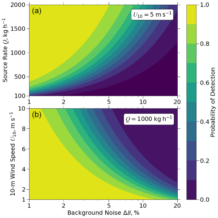
Figure 5Probability of detection (J > 0.1) for point sources calculated using Eq. (2) as a function of background noise (Eq. 1): source rate (a) and 10 m wind speed (b).
4.2 Source rate estimation
Figure 6 shows the source rate estimates for the complete U-Plume workflow, starting with the plume imagery and applying either the CNN or the IME method for source rate quantification. We restrict our analysis to plumes with a Jaccard score less than 0.1 to enable generalization for instruments with less background noise than GHGSat-C1 (such as GHGSat-C2), or we restrict it to the use of improved filtering methods (such as requiring a minimum number of plume pixels). Results are for the augmented dataset covering the 100–2000 kg h−1 range but trained only over the 500–2000 kg h−1 range. We assume no error in wind speed for now.
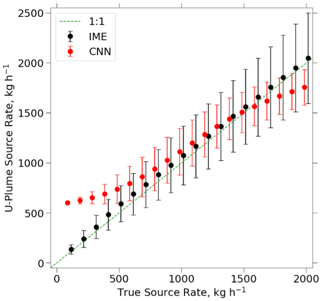
Figure 6Source rate estimates from the alternative CNN and IME methods (Fig. 2) for point sources emitting in the 100–2000 kg h−1 range (discrete 100 kg h−1 bins) in the augmented test dataset. The methods were trained with source rates in the 500–2000 kg h−1 range. Only images with Jaccard scores less than 0.1 are processed. Error bars show 1 standard deviation of the estimates.
The CNN method has a smoothing bias where low source rates are overestimated and high source rates are underestimated. This smoothing towards the mean is a common issue in machine learning methods and appears in the work of Jongaramrungruang et al. (2022) and Joyce et al. (2023). In addition, the CNN method is unable to extrapolate outside its training range. By contrast, the physically based IME method can successfully fit source rates down to 100 kg h−1 as long as the plumes are detectable. Discussion from this point forward will focus on the IME method as it performs better than the CNN method over the full range of source rates. We retain the CNN method as an option in the U-Plume algorithm because it offers an alternative source rate estimate for verification purposes and because it could be improved in the future with a more extensive training dataset. A potential avenue for future work would be to test other CNN architectures and expand training data to include the full range of possible source rates.
4.3 Error analysis
The uncertainty in source rate estimates using U-Plume with the IME method can be expressed as the relative error standard deviation (σQ) of the U-Plume estimate versus the true value. It has two independent components: (1) the error in the U-Plume algorithm, including the masking process and the IME parameterization (σQ,M), and (2) the error in 10 m wind speed (σQ,U). Here, we derive expressions for σQ,M and σQ,U and add them in quadrature to quantify the overall error and determine the driving factors.
The relative error standard deviation σQ,M from the U-Plume algorithm can be parameterized using the augmented test dataset binned according to point-source observability Ops, following the approach in Sect. 4.2 that only uses bins with > 50 positive detections (J > 0.1). Figure 7 shows the relative error standard deviation plotted against Ops.
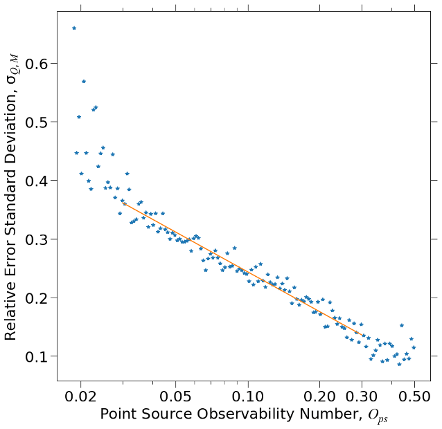
Figure 7Relative error in source rate estimation by the U-Plume algorithm. The figure shows the relative error standard deviation σQ,M versus the dimensionless point-source-observability number Ops (Eq. 6). Errors are calculated for point sources emitting in the 100–2000 kg h−1 range (discrete 100 kg h−1 bins) in the augmented test dataset, excluding error in wind speed (where the error is calculated separately – see text). Errors from individual images are binned according to the values of their point-source observability (Eq. 6) when Ops=0.005–0.5 into 201 log-spaced intervals. The orange line represents a reduced-major-axis (RMA) regression fit (R2=0.89) for σQ,M versus Ops (Eq. 8).
Fitting the error to log (Ops) yields
When Ops < 0.02, the probability of detection is less than 10 % (Sect. 4.1). The relative error standard deviation reaches a minimum of 10 % for highly observable plumes (Ops > 0.3), reflecting the irreducible error inherent to the IME method.
Uncertainty in wind speed adds another source of error. Let σU (m s−1) denote the error standard deviation in the 10 m wind speed U10. Substituting into Eqs. (4) and (5) yields a corresponding relative error standard deviation σQ,U for the inferred IME source rate Q:
Wind speed data may be available locally or from meteorological analysis datasets. A global default option is the NASA Goddard Earth Observing System Forward Processing (GEOS-FP) data, which is publicly available on a 0.25°×0.3125° grid with a 1 h temporal resolution. Varon et al. (2018) estimated an error standard deviation of σU=2 m s−1 for the GEOS-FP data, independent of wind speed magnitude, through comparison with 5 min observations at US airports. Substituting into Eq. (8) indicates a maximum relative error standard deviation of 66 % at low wind speed, which decreases with increasing wind speed. At high wind speeds, the error becomes small; however, the IME is then small, meaning that the masking error is large, as indicated by the inverse dependence of point-source observability on wind speed (Eq. 6 and Fig. 7).
Adding the error variances from Eqs. (8) and (9) in quadrature gives the total relative error variance for the estimated sources rates from the U-Plume algorithm (including the error in wind speed), which is defined as
Figure 8 shows the total relative error standard deviation σQ as a function of background noise ΔB, source rate Q, and 10 m wind speed U10, calculated using Eq. (10) under common observing conditions. Equation (10) can be used to calculate the values using any desired combination within the limits of the composed equations. The total relative error standard deviation increases linearly with log (ΔB), decreases linearly with log (Q), and reaches a minimum when U10=4 m s−1.

Figure 8Total relative error standard deviation σQ for point-source rate estimates from the U-Plume algorithm with the IME method (Eq. 9) shown as a function of three variables: background noise ΔB (%), source rate Q (kg h−1), and 10 m wind speed U10 (m s−1). The dashed orange line represents the probability of point-source detection calculated with Eq. (6).
In Fig. 9, the dependence of the total relative error standard deviation on wind speed is partitioned further into the contributions from the U-Plume algorithm and wind speed errors. The error contribution from the U-Plume algorithm increases with rising wind speed because methane enhancements in the plume become smaller, but this levels off at high wind speeds as the plumes are increasingly likely to be undetected instead. The error contribution from wind speed decreases with rising wind speed. The total error is dominated by wind speed when U10 < 4 m s−1 and by the U-Plume algorithm when U10 > 4 m s−1. Considering the range of values of ΔB and Q in our dataset, we find that the crossover between the two regimes occurs at 2–4 m s−1, which can be regarded as an optimum wind speed range for plume quantification.
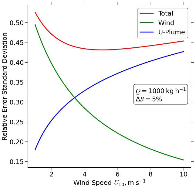
Figure 9Dependence of errors in point-source estimates on wind speed. This figure shows the relative error standard deviation for the source rate estimates inferred from U-Plume, with the IME method (Eq. 10) illustrated as a function of 10 m wind speed (U10). The total relative error standard deviation σQ is shown as the red line (also shown in as Fig. 8) and is decomposed into the contributions from errors in the U-Plume algorithm (σQ,M; Eq. 8) and errors in wind speed (σU; Eq. 9).
We developed the U-Plume algorithm for automated detection and quantification of point-source rates from high-resolution satellite imagery of atmospheric column concentrations. Our work was motivated by the need for fast identification of plumes in the operational processing of the vast amounts of methane data from the rapidly expanding GHGSat constellation and other satellite instruments targeting methane point sources. With instrument-specific training, this method can also be applied to any chemically inert plumes, such as those of CO2, due to the inherent similarity in the physics governing plume formation and transport.
U-Plume involves two steps. The first step involves a U-Net machine learning architecture for plume detection and delineation (masking) in noisy satellite images. The resulting plume mask is then used together with wind speed information in a second step of source rate quantification using either a convolutional neural network (CNN) or a physically based integrated mass enhancement (IME) method. Having both the plume mask and source rate information available from the U-Plume output is important for visualization, quality control, and pinpointing the source location. The end-to-end algorithm can process 62 images per second on a single core.
We trained U-Plume using an ensemble of plume-free observation images from the GHGSat-C1 satellite instrument covering a range of surfaces from homogeneous to highly heterogeneous and superimposing instantaneous methane plumes with known point-source rates from large-eddy simulations. Evaluation using data unseen by the model during the training process shows that successful plume detection and masking are strongly dependent on four state variables: instrument background noise ΔB, source rate Q, 10 m wind speed U10, and pixel resolution W. We combine these variables into a new dimensionless-number metric, point-source observability , and show that this metric can successfully predict the ability of the GHGSat-C1 imager to detect plumes and quantify source rates under given observing conditions. As it is dependent on the fundamental state variables of the enhancement produced by a methane point source, we expect that point-source observability will be a valuable metric for evaluating the detectability and quantification accuracy of other point-source imagers after appropriate tuning. For example, it can assist in determining when automation is possible for a given target detection level. For the GHGSat-C2 instruments with ΔB < 1 %, we thus expect that U-Plume will reliably detect and quantify point sources when Q > 400 kg h−1 and U=5 m s−1. For reference, GHGSat's manual plume detection method has achieved a 50 % probability of detection at 3 m s−1 and 117 kg h−1 in a self-administered controlled release campaign (https://go.ghgsat.com/validation-and-metrics-for-emissions-detection-by-satellite, last access: 29 April 2024) and detected the only emission less than 200 kg h−1 in a third-party-organized single-blind campaign (Sherwin, 2023). U-Plume's value lies in its ability to process large sets of plume data rather than in its ability to push the limits of detectability. Human operators with knowledge of point-source locations would be expected to have a greater ability to detect small sources (Sherwin et al., 2023).
We find that the physically based IME method is superior to the CNN method when it comes to inferring point-source rates from plume masks. The CNN exhibits high bias for low source rates and low bias for high source rates, as is typical of machine learning methods. The superiority of the IME method would be expected considering that there is a simple physically based linear relationship between plume mass and source rate modulated by wind speed. Although a CNN method may not require information on wind speed, such information is always available – either from local measurements or from regional/global databases.
We developed an end-to-end error model for the point-source rates inferred from U-Plume as a function of Ops. We find that at low wind speeds, the error is dominated by wind speed, whereas at higher wind speeds, the error is dominated by the U-Plume algorithm. The U10 value at which this shift occurs is typically between 2–4 m s−1. This also represents an optimal wind speed range for plume detection and quantification.
U-Plume thus offers a capable tool for fast automated processing of vast amounts of satellite imagery to detect plumes from point sources and quantify point-source rates. As satellite observations continue to improve in their ability to decrease background noise, the capability of U-Plume in detecting and quantifying points sources will correspondingly increase.
The model weights as well as both the original training data and the augmented test dataset are available through Harvard Dataverse (https://doi.org/10.7910/DVN/YFRQU4, Bruno, 2023).
JHB developed the U-Plume workflow and the code for image creation, network training, and error analysis. DJV ran the large-eddy simulations used in image creation. DJJ and DJ assisted in the project direction and formulation of the point-source-observability metric. JHB wrote the manuscript with comments and revisions from all authors.
At least one of the (co-)authors is a member of the editorial board of Atmospheric Measurement Techniques. The peer-review process was guided by an independent editor, and the authors also have no other competing interests to declare.
Publisher's note: Copernicus Publications remains neutral with regard to jurisdictional claims made in the text, published maps, institutional affiliations, or any other geographical representation in this paper. While Copernicus Publications makes every effort to include appropriate place names, the final responsibility lies with the authors.
Daniel J. Jacob acknowledges funding from the NASA Carbon Monitoring System. We thank one of the anonymous reviewers for identifying a coding error in the original version.
This research has been supported by NASA Carbon Monitoring System (grant no. 80NSSC21K1057) and the GHGSat Inc.
This paper was edited by Natalya Kramarova and reviewed by three anonymous referees.
Beirle, S., Borger, C., Dörner, S., Eskes, H., Kumar, V., de Laat, A., and Wagner, T.: Catalog of NOx emissions from point sources as derived from the divergence of the NO2 flux for TROPOMI, Earth Syst. Sci. Data, 13, 2995–3012, https://doi.org/10.5194/essd-13-2995-2021, 2021.
Bovensmann, H., Buchwitz, M., Burrows, J. P., Reuter, M., Krings, T., Gerilowski, K., Schneising, O., Heymann, J., Tretner, A., and Erzinger, J.: A remote sensing technique for global monitoring of power plant CO2 emissions from space and related applications, Atmos. Meas. Tech., 3, 781–811, https://doi.org/10.5194/amt-3-781-2010, 2010.
Bruno, J.: U-Plume Training Data, V2, Harvard Dataverse [data set], https://doi.org/10.7910/DVN/YFRQU4, 2023.
Buchwitz, M., Schneising, O., Reuter, M., Heymann, J., Krautwurst, S., Bovensmann, H., Burrows, J. P., Boesch, H., Parker, R. J., Somkuti, P., Detmers, R. G., Hasekamp, O. P., Aben, I., Butz, A., Frankenberg, C., and Turner, A. J.: Satellite-derived methane hotspot emission estimates using a fast data-driven method, Atmos. Chem. Phys., 17, 5751–5774, https://doi.org/10.5194/acp-17-5751-2017, 2017.
Clarisse, L., Van Damme, M., Clerbaux, C., and Coheur, P.-F.: Tracking down global NH3 point sources with wind-adjusted superresolution, Atmos. Meas. Tech., 12, 5457–5473, https://doi.org/10.5194/amt-12-5457-2019, 2019.
Cusworth, D. H., Jacob, D. J., Varon, D. J., Chan Miller, C., Liu, X., Chance, K., Thorpe, A. K., Duren, R. M., Miller, C. E., Thompson, D. R., Frankenberg, C., Guanter, L., and Randles, C. A.: Potential of next-generation imaging spectrometers to detect and quantify methane point sources from space, Atmos. Meas. Tech., 12, 5655–5668, https://doi.org/10.5194/amt-12-5655-2019, 2019.
Cusworth, D. H., Duren, R. M., Thorpe, A. K., Olson-Duvall, W., Heckler, J., Chapman, J. W., Eastwood, M. L., Helmlinger, M. C., Green, R. O., Asner, G. P., Dennison, P. E., and Miller, C. E.: Intermittency of Large Methane Emitters in the Permian Basin, Environ. Sci. Tech. Let., 8, 567–573, https://doi.org/10.1021/acs.estlett.1c00173, 2021.
Dammers, E., McLinden, C. A., Griffin, D., Shephard, M. W., Van Der Graaf, S., Lutsch, E., Schaap, M., Gainairu-Matz, Y., Fioletov, V., Van Damme, M., Whitburn, S., Clarisse, L., Cady-Pereira, K., Clerbaux, C., Coheur, P. F., and Erisman, J. W.: NH3 emissions from large point sources derived from CrIS and IASI satellite observations, Atmos. Chem. Phys., 19, 12261–12293, https://doi.org/10.5194/acp-19-12261-2019, 2019.
de Foy, B., Lu, Z., Streets, D. G., Lamsal, L. N., and Duncan, B. N.: Estimates of power plant NOx emissions and lifetimes from OMI NO2 satellite retrievals, Atmos. Environ., 116, 1–11, https://doi.org/10.1016/j.atmosenv.2015.05.056, 2015.
Duren, R. M., Thorpe, A. K., Foster, K. T., Rafiq, T., Hopkins, F. M., Yadav, V., Bue, B. D., Thompson, D. R., Conley, S., Colombi, N. K., Frankenberg, C., McCubbin, I. B., Eastwood, M. L., Falk, M., Herner, J. D., Croes, B. E., Green, R. O., and Miller, C. E.: California's methane super-emitters, Nature, 575, 180–184, https://doi.org/10.1038/s41586-019-1720-3, 2019.
Ehret, T., De Truchis, A., Mazzolini, M., Morel, J.-M., d'Aspremont, A., Lauvaux, T., Duren, R., Cusworth, D., and Facciolo, G.: Global Tracking and Quantification of Oil and Gas Methane Emissions from Recurrent Sentinel-2 Imagery, Environ. Sci. Technol., 56, 10517–10529, https://doi.org/10.1021/acs.est.1c08575, 2022.
Fioletov, V. E., McLinden, C. A., Krotkov, N., and Li, C.: Lifetimes and emissions of SO2 from point sources estimated from OMI, Geophys. Res. Lett., 42, 1969–1976, https://doi.org/10.1002/2015GL063148, 2015.
Guanter, L., Irakulis-Loitxate, I., Gorroño, J., Sánchez-García, E., Cusworth, D. H., Varon, D. J., Cogliati, S., and Colombo, R.: Mapping methane point emissions with the PRISMA spaceborne imaging spectrometer, Remote Sens. Environ., 265, 112671, https://doi.org/10.1016/j.rse.2021.112671, 2021.
Irakulis-Loitxate, I., Guanter, L., Liu, Y.-N., Varon, D. J., Maasakkers, J. D., Zhang, Y., Chulakadabba, A., Wofsy, S. C., Frankenberg, C., Thorpe, A. K., Thompson, D. R., Hulley, G., Kort, E. A., Vance, N., Borchardt, J., Krings, T., Gerilowski, K., Sweeney, C., Conley, S., Bue, B. D., Aubrey, A. D., Hook, S., and Green, R. O.: Airborne methane remote measurements reveal heavy-tail flux distribution in Four Corners region, P. Natl. Acad. Sci. USA, 113, 9734–9739, https://doi.org/10.1073/pnas.1605617113, 2016.
Irakulis-Loitxate, I., Guanter, L., Liu, Y.-N., Varon, D. J., Maasakkers, J. D., Zhang, Y., Chulakadabba, A., Wofsy, S. C., Thorpe, A. K., Duren, R. M., Frankenberg, C., Lyon, D., Cusworth, D. H., Zhang, Y., Segl, K., Gorroño, J., Sánchez-García, E., Sulprizio, M. P., Aben, I., and Jacob, D. J.: Satellite-based characterization of methane point sources in the Permian Basin, EGU General Assembly 2021, online, 19–30 Apr 2021, EGU21-15877, https://doi.org/10.5194/egusphere-egu21-15877, 2021.
Jacob, D. J., Turner, A. J., Maasakkers, J. D., Sheng, J., Sun, K., Liu, X., Chance, K., Aben, I., McKeever, J., and Frankenberg, C.: Satellite observations of atmospheric methane and their value for quantifying methane emissions, Atmos. Chem. Phys., 16, 14371–14396, https://doi.org/10.5194/acp-16-14371-2016, 2016.
Jacob, D. J., Varon, D. J., Cusworth, D. H., Dennison, P. E., Frankenberg, C., Gautam, R., Guanter, L., Kelley, J., McKeever, J., Ott, L. E., Poulter, B., Qu, Z., Thorpe, A. K., Worden, J. R., and Duren, R. M.: Quantifying methane emissions from the global scale down to point sources using satellite observations of atmospheric methane, Atmos. Chem. Phys., 22, 9617–9646, https://doi.org/10.5194/acp-22-9617-2022, 2022.
Jadon, S.: A survey of loss functions for semantic segmentation, in: 2020 IEEE Conference on Computational Intelligence in Bioinformatics and Computational Biology (CIBCB), virtual, 27–29 October 2020, 1–7, https://doi.org/10.1109/CIBCB48159.2020.9277638, 2020.
Jervis, D., McKeever, J., Durak, B. O. A., Sloan, J. J., Gains, D., Varon, D. J., Ramier, A., Strupler, M., and Tarrant, E.: The GHGSat-D imaging spectrometer, Atmos. Meas. Tech., 14, 2127–2140, https://doi.org/10.5194/amt-14-2127-2021, 2021.
Jongaramrungruang, S., Frankenberg, C., Matheou, G., Thorpe, A. K., Thompson, D. R., Kuai, L., and Duren, R. M.: Towards accurate methane point-source quantification from high-resolution 2-D plume imagery, Atmos. Meas. Tech., 12, 6667–6681, https://doi.org/10.5194/amt-12-6667-2019, 2019.
Jongaramrungruang, S., Thorpe, A. K., Matheou, G., and Frankenberg, C.: MethaNet – An AI-driven approach to quantifying methane point-source emission from high-resolution 2-D plume imagery, Remote Sens. Environ., 269, 112809, https://doi.org/10.1016/j.rse.2021.112809, 2022.
Joyce, P., Ruiz Villena, C., Huang, Y., Webb, A., Gloor, M., Wagner, F. H., Chipperfield, M. P., Barrio Guilló, R., Wilson, C., and Boesch, H.: Using a deep neural network to detect methane point sources and quantify emissions from PRISMA hyperspectral satellite images, Atmos. Meas. Tech., 16, 2627–2640, https://doi.org/10.5194/amt-16-2627-2023, 2023.
Krings, T., Gerilowski, K., Buchwitz, M., Reuter, M., Tretner, A., Erzinger, J., Heinze, D., Pflüger, U., Burrows, J. P., and Bovensmann, H.: MAMAP – a new spectrometer system for column-averaged methane and carbon dioxide observations from aircraft: retrieval algorithm and first inversions for point source emission rates, Atmos. Meas. Tech., 4, 1735–1758, https://doi.org/10.5194/amt-4-1735-2011, 2011.
Krings, T., Gerilowski, K., Buchwitz, M., Hartmann, J., Sachs, T., Erzinger, J., Burrows, J. P., and Bovensmann, H.: Quantification of methane emission rates from coal mine ventilation shafts using airborne remote sensing data, Atmos. Meas. Tech., 6, 151–166, https://doi.org/10.5194/amt-6-151-2013, 2013.
Maasakkers, J. D., Varon, D. J., Elfarsdóttir, A., McKeever, J., Jervis, D., Mahapatra, G., Pandey, S., Lorente, A., Borsdorff, T., Foorthuis, L. R., Schuit, B. J., Tol, P., van Kempen, T. A., van Hees, R., and Aben, I.: Using satellites to uncover large methane emissions from landfills, Science Advances, 8, eabn9683, https://doi.org/10.1126/sciadv.abn9683, 2022.
McLinden, C. A., Fioletov, V., Krotkov, N. A., Li, C., Boersma, K. F., and Adams, C.: A Decade of Change in NO2 and SO2 over the Canadian Oil Sands as Seen from Space, Environ. Sci. Technol., 50, 331–337, https://doi.org/10.1021/acs.est.5b04985, 2016.
Nassar, R., Hill, T. G., McLinden, C. A., Wunch, D., Jones, D. B. A., and Crisp, D.: Quantifying CO2 Emissions From Individual Power Plants From Space, Geophys. Res. Lett., 44, 10045–10053, https://doi.org/10.1002/2017GL074702, 2017.
Noppen, L., Clarisse, L., Tack, F., Ruhtz, T., Merlaud, A., Van Damme, M., Van Roozendael, M., Schuettemeyer, D., and Coheur, P.: Constraining industrial ammonia emissions using hyperspectral infrared imaging, Remote Sens. Environ., 291, 113559, https://doi.org/10.1016/j.rse.2023.113559, 2023.
Pommier, M., McLinden, C. A., and Deeter, M.: Relative changes in CO emissions over megacities based on observations from space, Geophys. Res. Lett., 40, 3766–3771, https://doi.org/10.1002/grl.50704, 2013.
Ramier, A., Girard, M., Jervis, M., MacLean, J.P, Marshall, D., McKeever J., Strupler, M., Tarrant, E., and Young, D.: High-Resolution Methane Detection with the GHGSat Constellation, in: GLOC 2023 conference proceedings, Oslo, Norway, 23–25 May 2023, 75002, 2023.
Rezvanbehbahani, S., Stearns, L. A., Keramati, R., Shankar, S., and van der Veen, C. J.: Significant contribution of small icebergs to the freshwater budget in Greenland fjords, Communications Earth & Environment, 1, 1–7, https://doi.org/10.1038/s43247-020-00032-3, 2020.
Ronneberger, O., Fischer, P., and Brox, T.: U-Net: Convolutional Networks for Biomedical Image Segmentation, in: Medical Image Computing and Computer-Assisted Intervention – MICCAI 2015, Cham, Munich, Germany, 5–9 October 2015, 234–241, https://doi.org/10.1007/978-3-319-24574-4_28, 2015.
Sherwin, E. D., Rutherford, J. S., Chen, Y., Aminfard, S., Kort, E. A., Jackson, R. B., and Brandt, A. R.: Single-blind validation of space-based point-source detection and quantification of onshore methane emissions, Sci. Rep., 13, 3836, https://doi.org/10.1038/s41598-023-30761-2, 2023.
Thorpe, A. K., Green, R. O., Thompson, D. R., Brodrick, P. G., Chapman, J. W., Elder, C. D., Irakulis-Loitxate, I., Cusworth, D. H., Ayasse, A. K., Duren, R. M., Frankenberg, C., Guanter, L., Worden, J. R., Dennison, P. E., Roberts, D. A., Chadwick, K. D., Eastwood, M. L., Fahlen, J. E., and Miller, C. E.: Attribution of individual methane and carbon dioxide emission sources using EMIT observations from space, Science Advances, 9, eadh2391, https://doi.org/10.1126/sciadv.adh2391, 2023.
Valin, L. C., Russell, A. R., and Cohen, R. C.: Variations of OH radical in an urban plume inferred from NO2 column measurements, Geophys. Res. Lett., 40, 1856–1860, https://doi.org/10.1002/grl.50267, 2013.
Varon, D. J., Jacob, D. J., McKeever, J., Jervis, D., Durak, B. O. A., Xia, Y., and Huang, Y.: Quantifying methane point sources from fine-scale satellite observations of atmospheric methane plumes, Atmos. Meas. Tech., 11, 5673–5686, https://doi.org/10.5194/amt-11-5673-2018, 2018.
Varon, D. J., McKeever, J., Jervis, D., Maasakkers, J. D., Pandey, S., Houweling, S., Aben, I., Scarpelli, T., and Jacob, D. J.: Satellite Discovery of Anomalously Large Methane Point Sources From Oil/Gas Production, Geophys. Res. Lett., 46, 13507–13516, https://doi.org/10.1029/2019GL083798, 2019.
Varon, D. J., Jacob, D. J., Jervis, D., and McKeever, J.: Quantifying Time-Averaged Methane Emissions from Individual Coal Mine Vents with GHGSat-D Satellite Observations, Environ. Sci. Technol., 54, 10246–10253, https://doi.org/10.1021/acs.est.0c01213, 2020.
Varon, D. J., Jervis, D., McKeever, J., Spence, I., Gains, D., and Jacob, D. J.: High-frequency monitoring of anomalous methane point sources with multispectral Sentinel-2 satellite observations, Atmos. Meas. Tech., 14, 2771–2785, https://doi.org/10.5194/amt-14-2771-2021, 2021.