the Creative Commons Attribution 4.0 License.
the Creative Commons Attribution 4.0 License.
 | 06 May 2024
An iterative algorithm to simultaneously retrieve aerosol extinction and effective radius profiles using CALIOP
Liang Chang
Jingjing Ren
Changrui Xiong
Lu Zhang
The Cloud-Aerosol Lidar with Orthogonal Polarization (CALIOP) on board the Cloud-Aerosol Lidar and Infrared Pathfinder Satellite Observation (CALIPSO) satellite has been widely used in climate and environment studies to obtain the vertical profiles of atmospheric aerosols. To retrieve the vertical profile of aerosol extinction, the CALIOP algorithm assumes column-averaged lidar ratios based on a clustering of aerosol optical properties measured at surface stations. On one hand, these lidar ratio assumptions may not be appropriate or representative at certain locations. One the other hand, the two-wavelength design of CALIOP has the potential to constrain aerosol size information, which has not been considered in the operational algorithm. In this study, we present a modified inversion algorithm to simultaneously retrieve aerosol extinction and effective radius profiles using two-wavelength elastic lidars such as CALIOP. Specifically, a lookup table is built to relate the lidar ratio with the Ångström exponent calculated using aerosol extinction at the two wavelengths, and the lidar ratio is then determined iteratively without a priori assumptions. The retrieved two-wavelength extinction at each layer is then converted to the particle effective radius assuming a lognormal distribution. The algorithm is tested on synthetic data, Raman lidar measurements and then finally the real CALIOP backscatter measurements. Results show improvements over the CALIPSO operational algorithm by comparing with ground-based Raman lidar profiles.
- Article
(7225 KB) - Full-text XML
- BibTeX
- EndNote


Atmospheric aerosols have important impacts on the physical and chemical processes in the atmosphere, as well as the climate system and public health. Optical properties of aerosols are critical in quantifying their radiative effects in the Earth's climate system. Moreover, the vertical distribution of aerosol properties, such as extinction coefficient and particle size, is one of the key elements to assess climate effect (IPCC, 2023). Direct aerosol radiative forcing, which plays an important role in the Earth's energy budget, is impacted by the vertical distribution of aerosols, especially that of absorbing aerosols (Goto et al., 2011; Eswaran et al., 2019; Zhang et al., 2022). The vertical profiles of aerosol optical properties are also essential in estimating the solar heating rate (Kudo et al., 2016) and in the establishment of aerosol parameterization schemes for satellite remote sensing (He et al., 2016). Although its importance is widely recognized, aerosol vertical distribution is very difficult to monitor globally. Using lidar is a major technique for obtaining the profiles of aerosol properties and has been used in ground-based and satellite remote sensing systems. In particular, spaceborne lidar is an effective way to observe the global distribution of aerosols. The Cloud-Aerosol Lidar with Orthogonal Polarization (CALIOP) on the CALIPSO (Cloud-Aerosol Lidar and Infrared Pathfinder Satellite Observation) satellite, the only long-term orbiting spaceborne lidar to date, was launched on 28 April 2006. CALIOP is a three-channel Mie scattering lidar system, which contains two wavelengths of 532 nm (perpendicular and parallel polarization channel) and 1064 nm. It is the first polarization lidar to provide three-channel elastic backscatter signals of global atmospheric measurements. The official aerosol retrieval algorithm of CALIOP involves three modules, namely the Selective Iterated BoundarY Locator (SIBYL), the Scene Classification Algorithm (SCA) and the Hybrid Extinction Retrieval Algorithm (HERA). HERA requires a lidar ratio (extinction-to-backscatter ratio of aerosols), which is provided by the SCA. The SCA uses three CALIOP channels (532 parallel, 532 nm perpendicular and 1064 nm channels) to obtain the lidar ratio from the six groups of assumed column-averaged lidar ratios based on a clustering of aerosol optical properties measured at surface stations (Winker et al., 2009).
The lidar ratio is dependent on the chemical composition, shape and particle size distribution of aerosols, as well as the lidar wavelength (Burton et al., 2012), which is a critical parameter required for solving the Mie scattering lidar equation using the Klett (Klett, 1985) or Fernald (Fernald, 1984) methods. Previous studies have developed algorithms to determine the lidar ratio iteratively for two-wavelength Mie scattering lidars. Potter (1987) first introduced the two-wavelength lidar inversion technique to retrieve the aerosol transmission with a constant lidar ratio in two independent wavelengths. Ackermann (1997, 1998) developed an iterative method to obtain the variable lidar ratio from two-component (i.e., molecule and aerosol) atmospheres by transcendental equations. Rajeev and Parameswaran (1998) proposed a new method using Mie-theory-calculated aerosol optical properties with a Junge distribution of aerosols to determine the lidar ratio by iteration. Lu et al. (2011) made an attempt to improve the two-wavelength lidar inversion by the iterative method but failed to consider the size distribution of aerosols, which may introduce uncertainties in the inversion. Moreover, these studies mostly only gave the aerosol extinction profile without retrieving the vertical distribution of aerosol size information. The algorithms were also mostly applied to theoretical data or ground lidar measurements. The application to space lidars such as CALIOP is challenging and thus limited.
In view of the above discussions, this study aims to provide a modified two-wavelength lidar inversion algorithm to retrieve the vertical distribution of both the aerosol extinction and the particle effective radius, avoiding the complex calculation confronted in the previous two-wavelength lidar inversion methods. The algorithm is tested on synthetic data and surface Raman lidar and is finally applied to CALIOP measurements in order to better demonstrate its operational feasibility. The paper proceeds with descriptions of the inversion algorithm in Sect. 2. Section 3 presents the application of the algorithm to the Raman lidar and CALIOP, with an analysis of retrieval uncertainties provided in Sect. 4. The study concludes in Sect. 5 with a brief discussion in the context of relevant lidar algorithms.
The modified inversion algorithm retrieves the profiles of the aerosol extinction and effective radius at two wavelengths by solving the lidar equation using the Fernald method (Fernald, 1984) with a lookup-table approach in the iteration procedure.
2.1 Solving the lidar equation
For each wavelength with a complete overlap between the fields of view of the laser and of the receiver, the lidar equation with calibration and range correction can be expressed as
where
In Eqs. (1)–(3), β′(R) is the attenuated backscatter coefficients (calibrated and range-corrected signal) from distance R; P(R) is the measured signal after background subtraction and artifact removal from distance R; E0 is the average laser energy for the single shot; ξ is the lidar system parameter; β(R) and σ(r) are the volume backscatter and extinction coefficient at range R and r, respectively; T2(R) is the two-way transmittance from the lidar to the scattering volume at range R; τ(R) is the optical depth at range R; and the subscripts m and p denote the portions of air molecules and aerosols, respectively.
In order to facilitate calculation, the transmittance of air molecules is separated from β′(R) to obtain E(R) as
As is well known, lidar back scatter signal is also subject to multiple-scattering effects. These effects are typically small for low to moderate aerosol loading and are only significant for optically thick clouds (Winker et al., 2009). Therefore, we neglect multiple-scattering effects here and consider the lidar ratio (S(R)) of aerosols to be range dependent in single-scatter approximation, which can be written as
In the following, we use the Fernald method (Ackermann, 1998) to obtain the aerosol extinction coefficient at distance R as
where
The backscatter and extinction coefficient of air molecules can be determined with Rayleigh scattering theory, with the observed atmospheric profile (Bodhaine et al., 1999) as
where P(R) and T(R) are the atmospheric pressure (hPa) and temperature (K) at distance R, respectively. Cs(λ) and kbω(λ) are the atmospheric molecular constants related to the wavelength λ. Hostetler et al. (2006) suggested the values of Cs(λ) and kbω(λ) to be 532 and 1064 nm as (K hPa−1 m−1), (K hPa−1 m−1), kbω (532 nm) =1.0313 and kbω (1604 nm) =1.0302.
Thus, the aerosol extinction coefficient profiles can be obtained by Eq. (6) with an unknown variable of the lidar ratio. The two-wavelength lidar can give two independent profiles of attenuated backscatter coefficients at different wavelengths, from which the aerosol extinction coefficient profiles can be calculated by assuming the lidar ratios at the two wavelengths.
For two wavelengths (λ1 and λ2), the Ångström exponent (AE) at distance R is defined as
Because AE is related to particle size distribution, which is a primary factor determining the lidar ratio, an AE–lidar ratio relationship can be established and used to determine the lidar ratio at each layer, which can then be used to retrieve aerosol extinction profiles from two-wavelength lidar measurements.
2.2 Lookup table
By assuming a spherical particle size distribution, the aerosol extinction coefficients and backscatter coefficients can be calculated by Eqs. (11)–(12):
where n(r) represents the volume size distribution of particles; rmax and rmin are the maximum and minimum of the particle radius, respectively; and Qe(λ,r) and Qb(λ,r) denote the extinction and backscatter efficiencies of the particle (the scatter factor of the particle at 180°) with size r at wavelength λ, respectively. The size parameter is defined as , where for typical aerosols, and thus Mie scattering theory (Mishchenko and Yang, 2018) can be applied.
As the information provided by two-wavelength lidar is limited, we assume the volume size distribution of aerosols conform to the lognormal distribution, and the size distribution is expressed as follows (Deshler et al., 2003; Hara et al., 2021):
where N is the total particle concentrations and r0 and sd are the median radius and the geometric standard deviation of aerosol size distribution, respectively. The particle size distribution is represented by its effective radius (re) defined as (Veselovskii et al., 2002; Di Girolamo et al., 2022)
For convenient calculation, we assume a constant sd for the each aerosol type, and the relationship between AE and re can be established with given r0 values.
We choose the six types of aerosols with their parameters in Table 1, which is consistent with the aerosol classification used in the operational algorithm of CALIOP (Winker et al., 2009). From Table 1, Type 3 denotes the scattering aerosols and Type 2 shows both strong scattering and absorption, whereas other types have moderate scattering or are absorbing. Combining Eqs. (5) and (10)–(14), the relationship between the Ångström exponent (AE) and lidar ratio (S), as well as that between AE and the particle effective radius (re), can be formulated as lookup tables for different refractive indices, as shown in Fig. 1. Note that in Fig. 1, it is easy to determine S532 nm, S1064 nm and re by the unique AE calculated from the lidar equation for a fixed aerosol type.
Table 1The aerosols parameters of the lookup table. mr denotes the real part of the refractive index, mi denotes the imaginary part of the refractive index and SD is the standard deviation of the lognormal size distribution.


Figure 1The lookup tables for (a) AE–effective radius, (b) AE–lidar ratio at 532 nm and (c) AE–lidar ratio at 1064 nm. The AE is calculated using 532 and 1064 nm aerosol extinction coefficients.
2.3 The iterative inversion procedure
After constructing the lookup table, we design the following iterative procedure to simultaneously retrieve aerosol extinction and effective radius profiles. Firstly, we calculate the extinction coefficients (σ532 nm and σ1064 nm) of two wavelengths (532 and 1064 nm) from an initial guess of the lidar ratios ( and ) by solving the lidar equation (Eq. 6), and then we obtain the Ångström exponent (AE) through Eq. (10). Secondly, the lookup tables are used to determine a set of new lidar ratios ( and ), which is used to calculate the new σ532 nm and σ1064 nm and Ångström exponent (AE′). This procedure is repeated until the difference between the updated AE′ and previous AE reduces to a very small value (e.g., 10−3). The final AE is converted to the effective radius from the AE–re lookup table, and the final values of σ532 nm, σ1064 nm, S532 nm, S1064 nm and re are the retrieved results of this layer. The above iterative algorithm is summarized in Fig. 2.

Figure 2Schematic of the inversion algorithm (532 nm and 1064 nm represent the two different wavelengths, respectively; S is the lidar ratio; σ is the aerosol extinction; AE is the Ångström index; re is the particle effective radius; S0 is the initial value of the lidar ratio; and S′ and AE′ are the lookup values of the lidar ratio and Ångström index, respectively).
Although in theory our algorithm can retrieve the aerosol extinction and effective radius at each layer, in reality the measurement noise may cause the inversion of certain layers to fail to converge. In these cases, we assume that this layer has the same aerosol type and size distribution as its adjacent layer, and then these two layers are combined into a new layer to continue with the inversion.
2.4 Test of the algorithm with synthetic data
For verifying the feasibility of the inversion algorithm, we first conduct some retrieval tests using synthetic data from Mie scattering and radiative transfer simulations. We assume a hypothesized profile of the effective radius and backscatter and extinction coefficients of the aerosols, and use the U.S. Standard Atmosphere model of 1976 (National Geophysical Data, 1992) for molecular scattering, and calculate the attenuated backscatter profiles according to the lidar equation. We then apply our algorithm to retrieve the aerosol property profiles from these simulated lidar signals and compare them with the initial assumptions.
We only present the results for the reflective aerosol model, and results for other aerosol types are similar. The simulated attenuated backscatter profiles for the two wavelengths are shown in Fig. 3, and the results of our inversion and their comparison with the assumed profiles are shown in Fig. 4. It is clearly seen that the results of the inversion are in good agreement with the assumed profiles. The MAPE (mean absolute percentage error) values between retrieved and assumed profiles of the extinction coefficient, average particle effective radius and lidar ratio are all below 0.1 %, which proves the validity of the algorithm in theory. Note that typically, the selection of aerosol type is critical as an incorrect assumption regarding the aerosol refractive index will result in divergence of the algorithm and thus yield no valid retrieval. This also helps us to determine the appropriate aerosol type, i.e., the type that yields the best retrieval results.
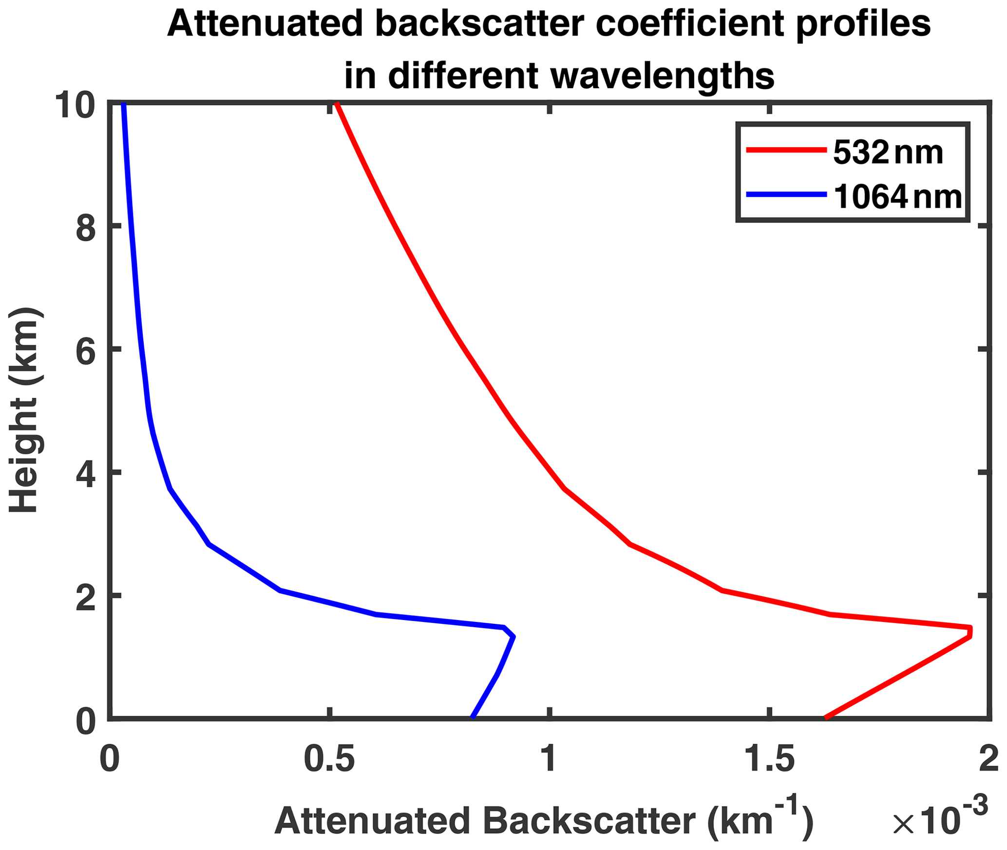
Figure 3The attenuated backscatter coefficient profiles at different wavelengths using synthetic data.
Before applying our algorithm to CALIOP measurements, we first use Raman lidar measurements to test its accuracy as Raman lidars can directly retrieve aerosol extinction profiles without assuming a lidar ratio.
3.1 Application to Raman lidar measurements
A Raman lidar (model LR231-D300, Raymetrics S.A., Greece) is installed on top of an eight-floor building at the Peking University site (39°59′ N, 116°18′ E; 53 m above sea level (m a.s.l.)). It can provide the extinction and backscatter coefficients at 532 nm by Raman inversion (Ansmann et al., 1990) without the need to assume the lidar ratio. To test our inversion algorithm, we apply it to the elastic backscatter signals at 532 and 1064 nm and compare the retrieved extinction profile at 532 nm with that retrieved with the Raman method. Note that the 1064 nm extinction is estimated using the Ångström relationship of Eq. (10) and we assume that the 532–1064 nm AE equals the 355–532 nm AE. We apply the modified inversion algorithm to the cases of four different aerosol types. To facilitate the determination of the initial value, we use the method of remodeling downward attenuated backscatter from ground-based lidar (Tao et al., 2008) to reconstruct the Raman lidar measurements at wavelengths of 532 and 1064 nm, which are shown in Figs. 5a, 6a, 7a and 8a.
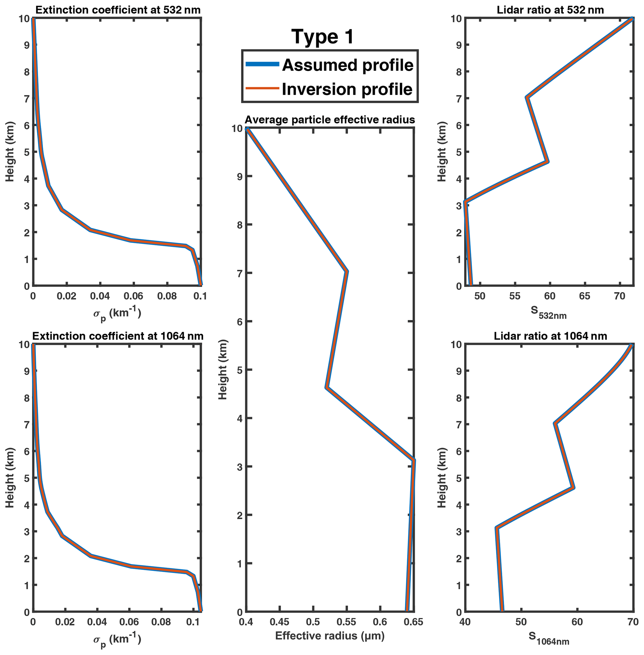

Figure 5(a) Remodeled downward attenuated backscatter profiles measured by Raman lidar in Peking University (PKU) on 1 December 2017; panels (b), (c) and (d) show the extinction profiles, lidar ratio profiles and particle radius profiles, respectively, inversed by the modified algorithm (red) and Raman method (blue).
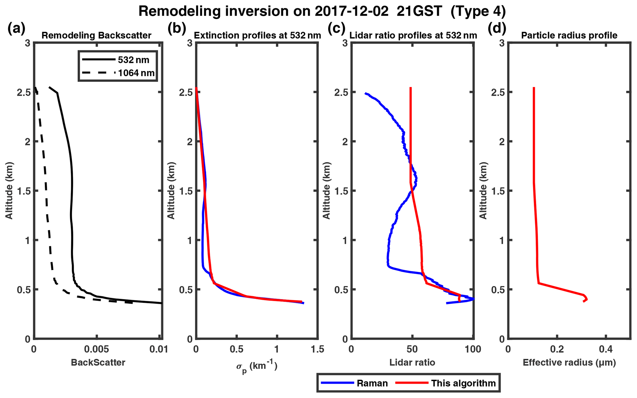

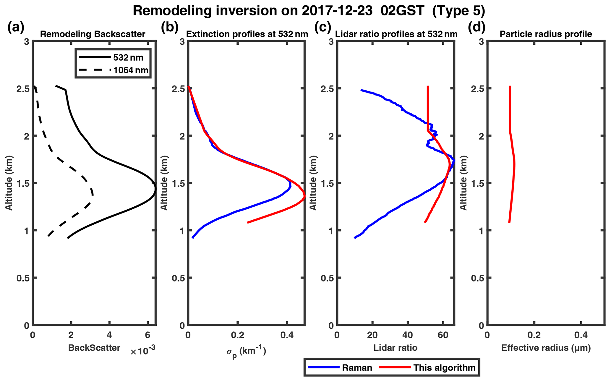
We examined four cases in December 2017, as shown in Figs. 5–8. The cases on 2 and 21 December 2017 both indicate that the extinction coefficient decreases sharply with altitude, and the maximum values occur near the ground (Figs. 6b, 7b). The other two cases on 1 and 23 December show the features of an elevated aerosol layer with maximum extinction found above the surface. In all four cases, our retrieval results (red curves) agree well with those retrieved by the Raman method, with MAPE less than 30 % in the extinction coefficient profiles. The lidar ratio profiles retrieved by our algorithm also agree well with those obtained from the Raman method in some ranges, except spikes at the highest or lowest point, which may be caused by the uncertainty of the boundary. The aerosol particle effective radius slightly increases with altitude, and the peak (corresponding to ∼ 0.1 µm) appears at ∼0.7 and ∼ 1.7 km on 1 and 23 December 2017 (Figs. 5d, 8d), respectively. Similar results were found by Zhang et al. (2009) and Cai et al. (2022) with aircraft measurements over Beijing and the Loess Plateau in China, respectively, which are mainly associated with long-range aerosol transport. The variability in particle effective radius profiles in Fig. 6d is a typical feature of a low (and stable) PBL (planetary boundary layer), which results in both particles and water vapor accumulating near the PBL top, and thus remarkable hygroscopic growth of particle size may occur (Yang et al., 2020). The case for 21 December (Fig. 7d) shows a relatively large particle size below ∼ 1.4 km but sharply decreases. This is likely related to the domination of local pollution and insignificant PBL temperature inversion (Li et al., 2022; Liu et al., 2009; Zhang et al., 2009).
3.2 Application to CALIOP measurements
We further apply our algorithm to real CALIOP measurements. To test its performance, we collocate CALIOP profiles with those from surface-based Raman lidar measurement within the European Aerosol Research Lidar Network (EARLINET; https://www.earlinet.org/index.php?id=earlinet_homepage, last access: 4 January 2022) (Matthias et al., 2004). Aerosol profiles from the Naples (southern Italy; 40.838° N, 14.183° E; 118 m a.s.l.), Evora (south-central Portugal; 38.5678° N, −7.9115° E; 293 m a.s.l.) and Warsaw (east-central Poland; 52.21° N, 20.98° E; 112 m a.s.l.) stations, which have the best match with CALIOP and high data quality in cloudless sky, are primarily used to validate the retrieval results. The CALIPSO overpass times for the chosen cases and the corresponding horizontal distances between the sub-satellite point and ground-based Raman lidar site are listed in Table 2.
Table 2Information about collocated EARLINET and CALIPSO cases.

To compare with the lidar returns measured by CALIOP (downward-looking) and ground-based Raman lidar (upward-looking), we still use the method of remodeling downward attenuated backscatter from ground-based lidar (Tao et al., 2008) to reconstruct the downward attenuated backscatter signals for the ground-based Raman lidar. The attenuated backscatter signals of CALIOP was averaged for 163 nearby sub-satellite point profiles (CALIPSO ground track range of about 30 km within 8 s) (Lu et al., 2011; Wang et al., 2007), obtained from CALIOP level-1B products, to improve the signal-to-noise ratio.
The attenuated backscatter profiles at 532 nm from CALIOP agree well with those from the Naples Raman lidar (NRL), as shown in Figs. 9a, 10a, 11a, 12a, 13a and 14a. The initial altitude of inversion (the upper boundary of the aerosol layer) is determined by the variation in the attenuated backscatter signal and volume linear depolarization ratio at 532 nm. Comparison between our inversion results, CALIOP operational results and Raman results is shown in Figs. 9c, 10c, 11c, 12c, 13c and 14c.
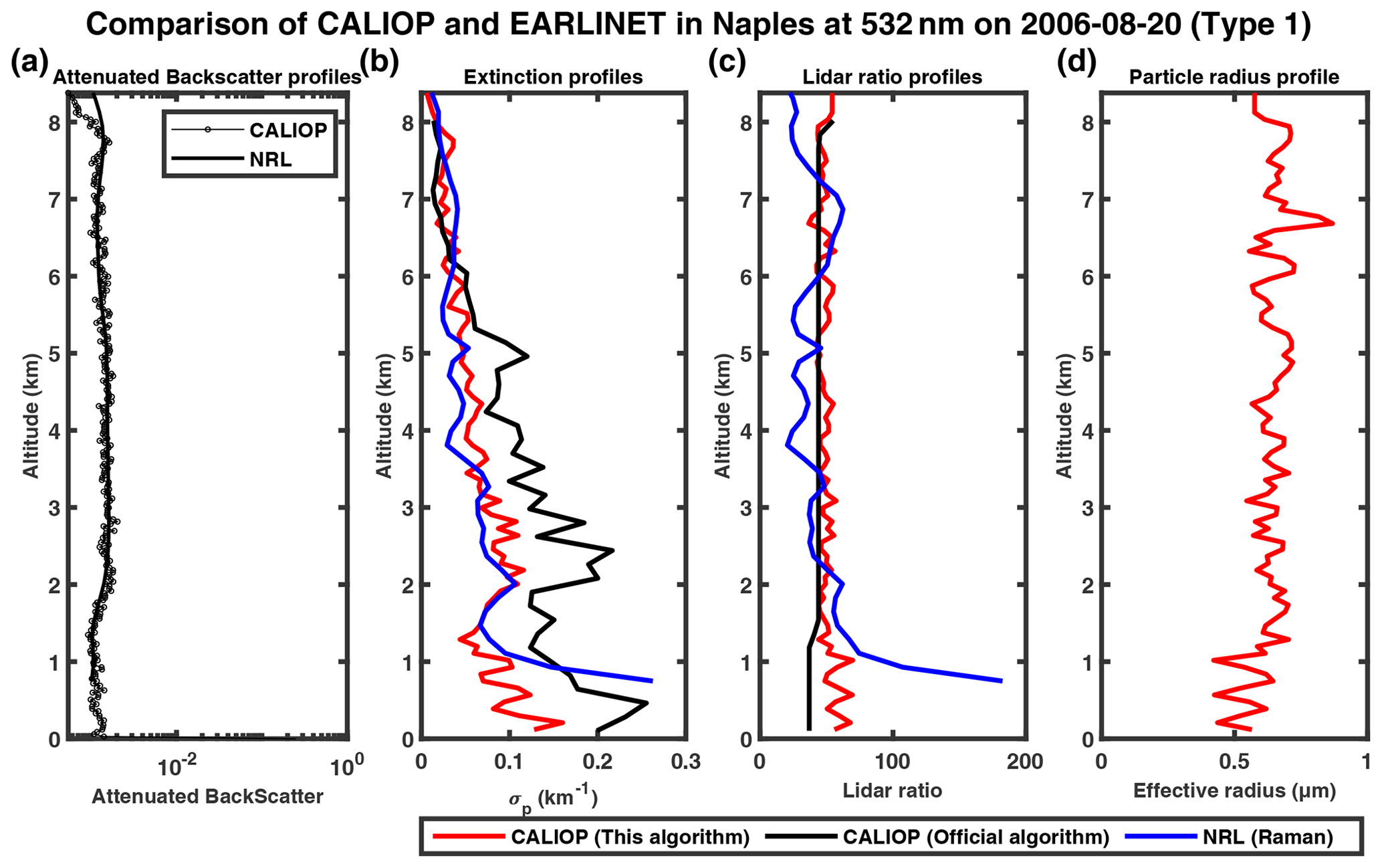
Figure 9The 532 and 1064 nm attenuated backscatter profiles measured by CALIOP (solid black line with circle marker) and NRL (remodeling, solid black line) on 20 August 2006 in a logarithmic scale in the horizontal direction (a); panels (b), (c) and (d) show the extinction profiles, lidar ratio profiles and particle radius profiles, respectively, provided by our inversion algorithm (red), CALIOP operational level-2 product (black) and EARLINET level-2 product (blue).
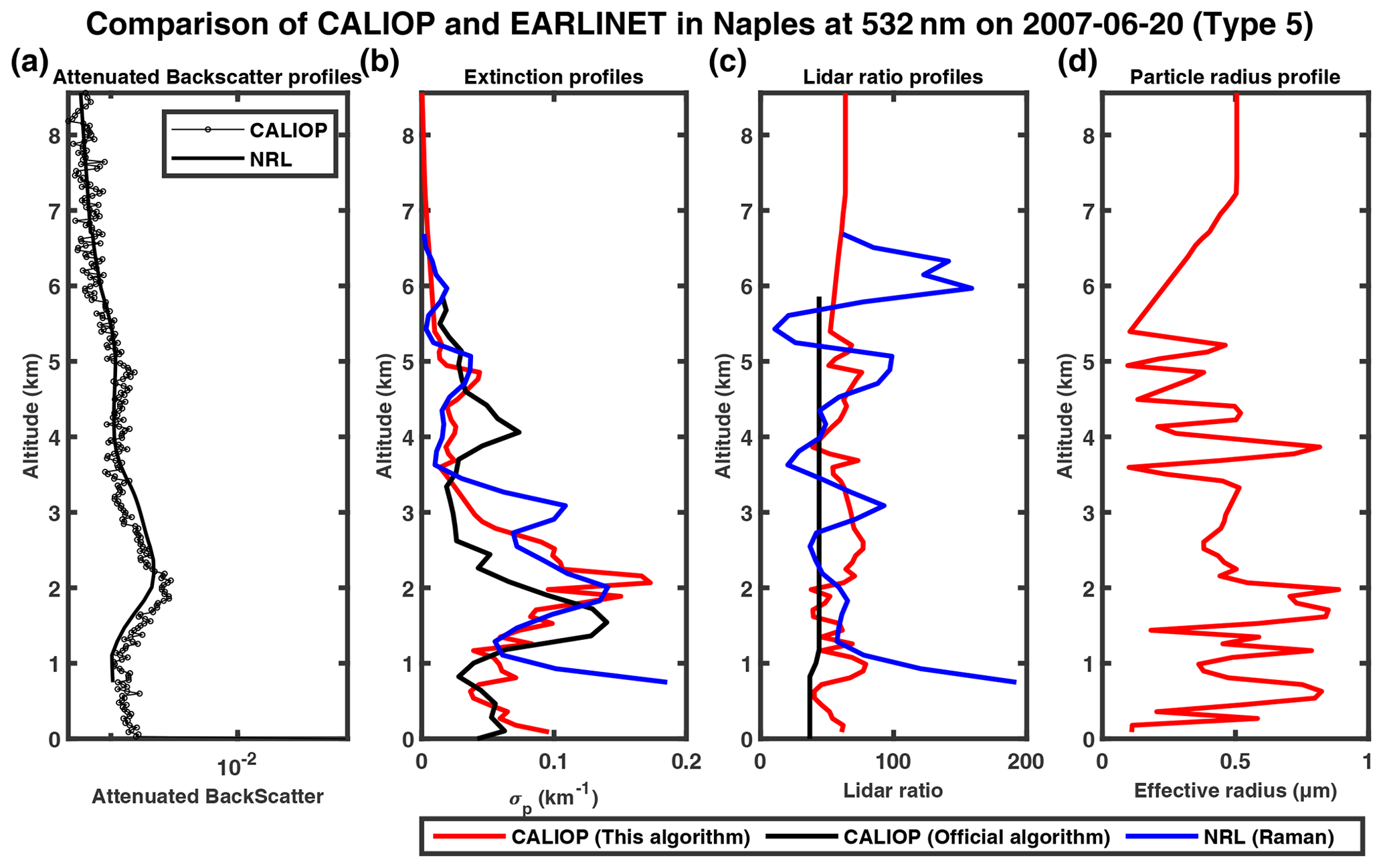


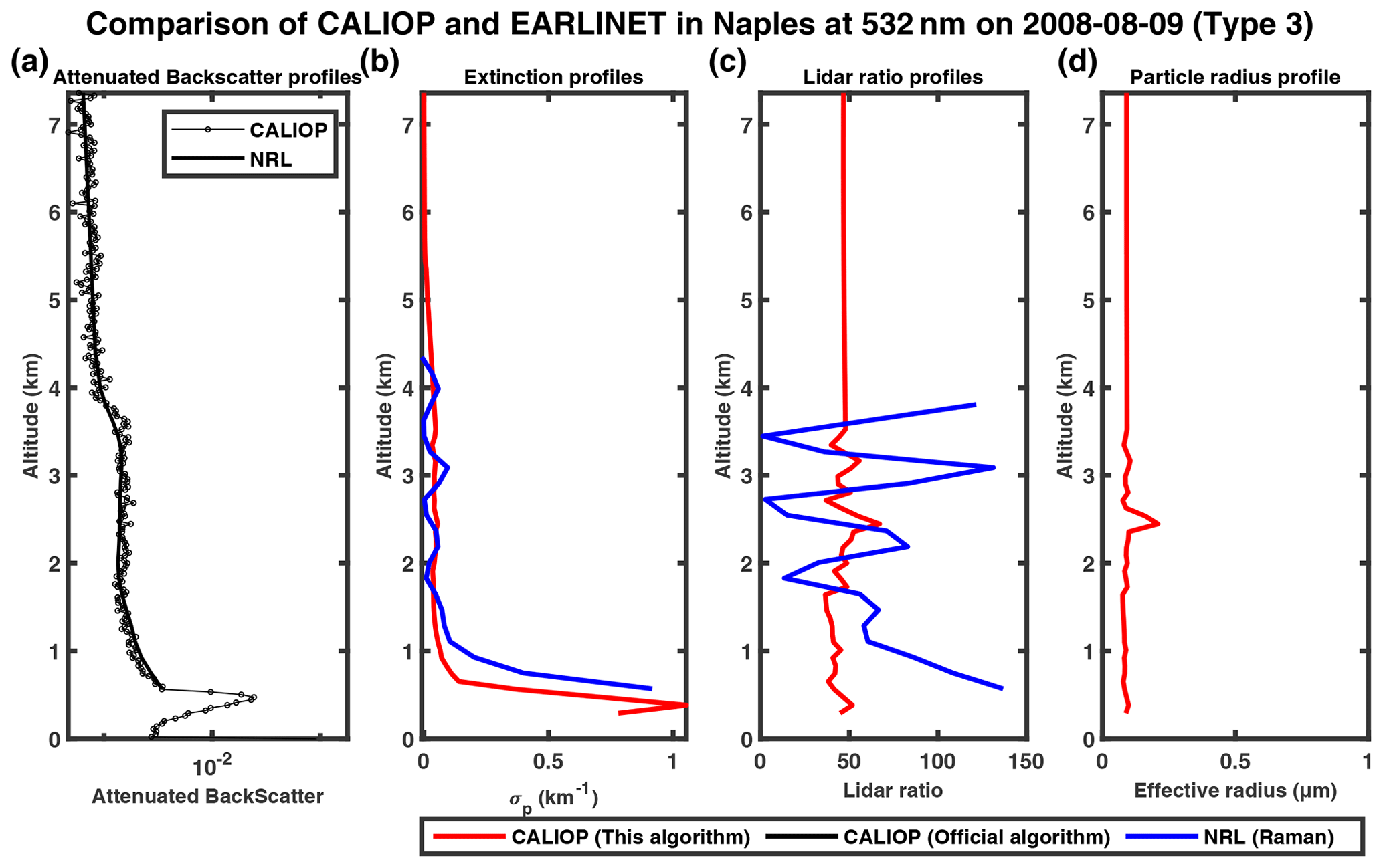
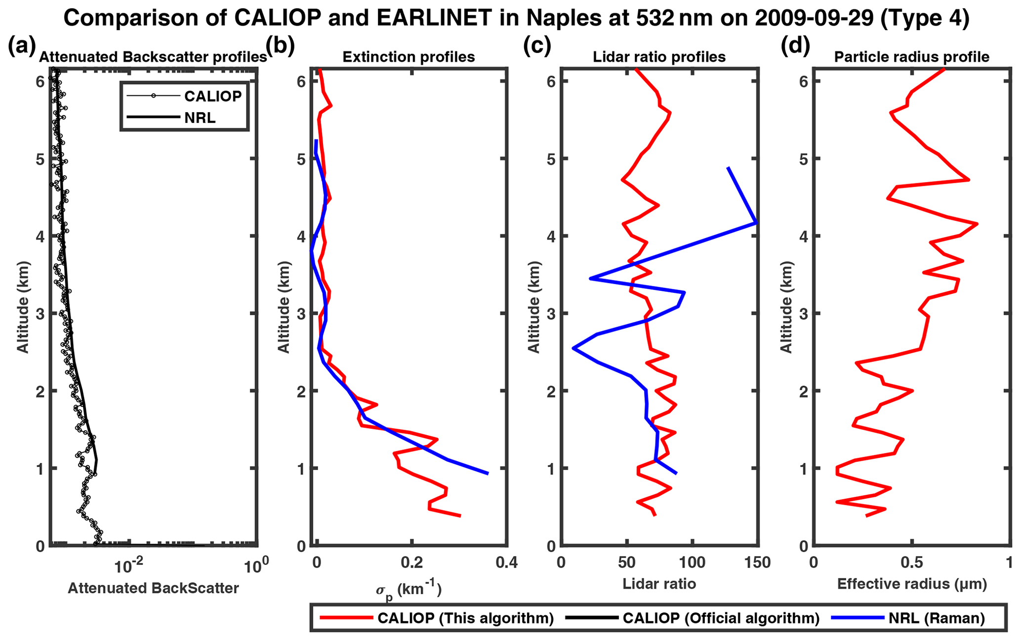
The CALIOP operational product only provides retrievals for three cases considered, namely 20 August 2006 and 20 June and 22 July 2007. In all three cases, the aerosol extinction profiles of our algorithm (red curve) appear to have better consistency with Raman lidar results, and our algorithm reduces the mean MAPE between the retrieval of extinction profiles in CALIOP and Raman lidar from 74 % (CALIOP operational product) to 37 %. Our algorithm successfully corrects the overestimation for the 20 August 2006 and 22 July 2007 cases. For the 20 June 2007 case, the operational results show a lower peak at ∼ 1.7 km and a secondary peak at ∼ 4 km, both of which are absent in the Raman profile, and our results agree well with Raman in both the shape and the magnitude. In the other three cases, CALIOP does not provide level-2 retrieval results. Our algorithm is able to perform retrievals, and the extinction profiles agree well with Raman lidar observations. Our retrievals do show more fluctuations compared to Raman lidar, possibly due to the noises in the attenuated backscatter profiles of CALIOP. Because Raman lidar does not provide retrieval of aerosol effective radius profiles, we compare the lidar ratio profiles by our algorithm and the Raman algorithm. Overall, our algorithm produces lidar ratios varying in a relatively small range around 50, whereas Raman lidar ratios can vary from ∼ 10 to 200. Also, the Raman lidar ratios tend to change sharply at the highest or lowest point, which may be caused by the inversion errors at the boundary. By removing these spikes, the differences in the lidar ratio between CALIOP and Raman are obviously reduced. In general, the aerosol particle effective radius increases with altitude, similarly to Figs. 5d and 8d, but the fluctuations in the profiles may also be caused by the noise in the CALIOP measurement.
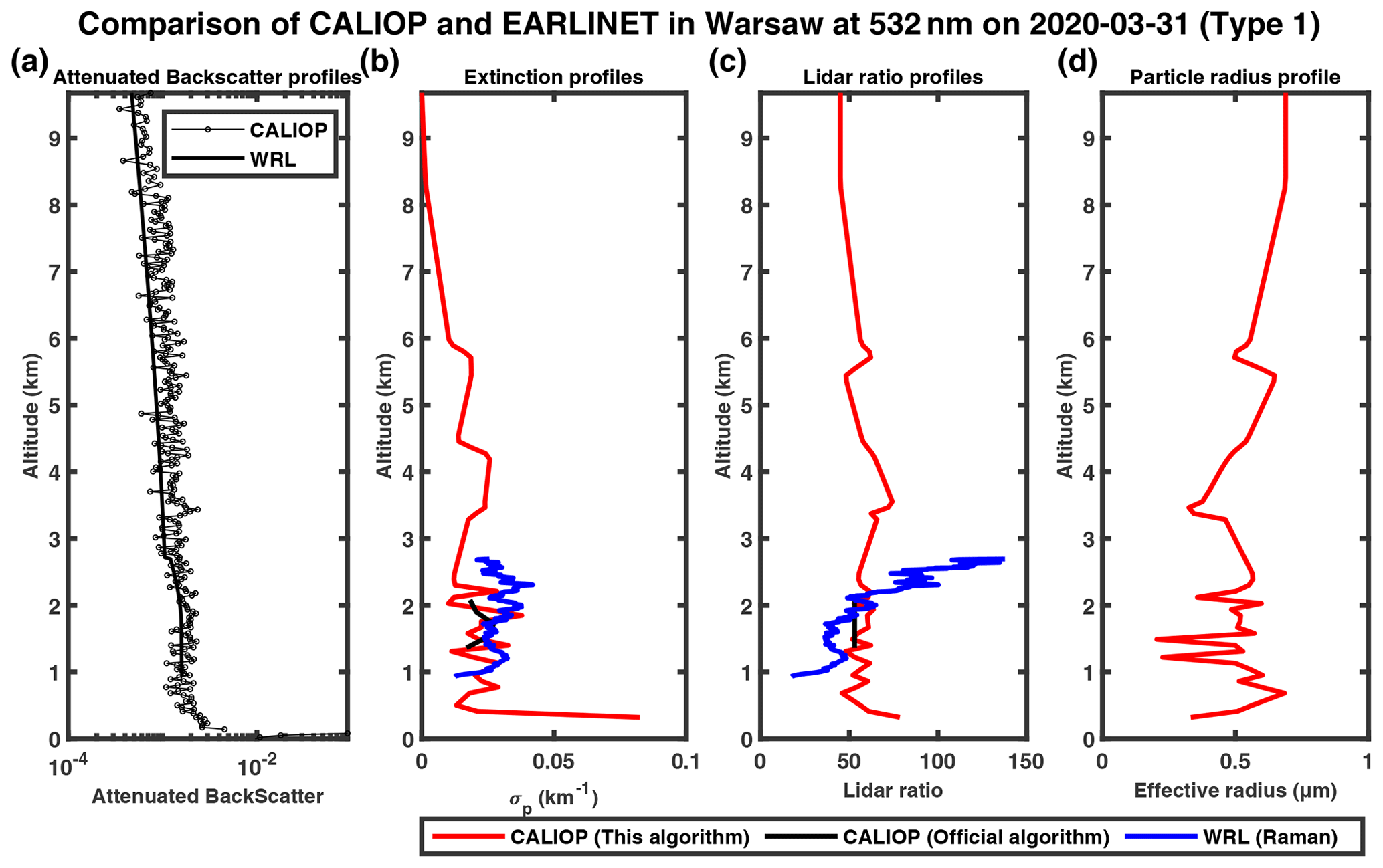
When examining the CALIOP backscatter measurements, we found that the backscatter signal at 1064 nm is often stronger than that at 532 nm after 2010, which is unphysical and possibly due to issues such as calibration and lidar degradation. As a result, the remodeled backscatter profiles of CALIOP appear noisier and do not exactly match those from Raman lidar for the Evora and Warsaw stations, which only have collocated measurements in 2019 and 2020 (Figs. 15a, 16a, 17a, 18a, 19a). Our retrieved extinction profiles also agree reasonably well with those by Raman lidar (Figs. 15b, 16b, 17b, 18b, 19b), with the lidar ratio profiles and aerosol particle effective radius profiles similar to the cases at Naples. By contrast, the extinction profiles of the official CALIPSO product show large deviations from the Raman profile with unphysical spikes (Fig. 16b), incomplete profiles (Figs. 17b, 18b) or no retrievals (Fig. 15b).
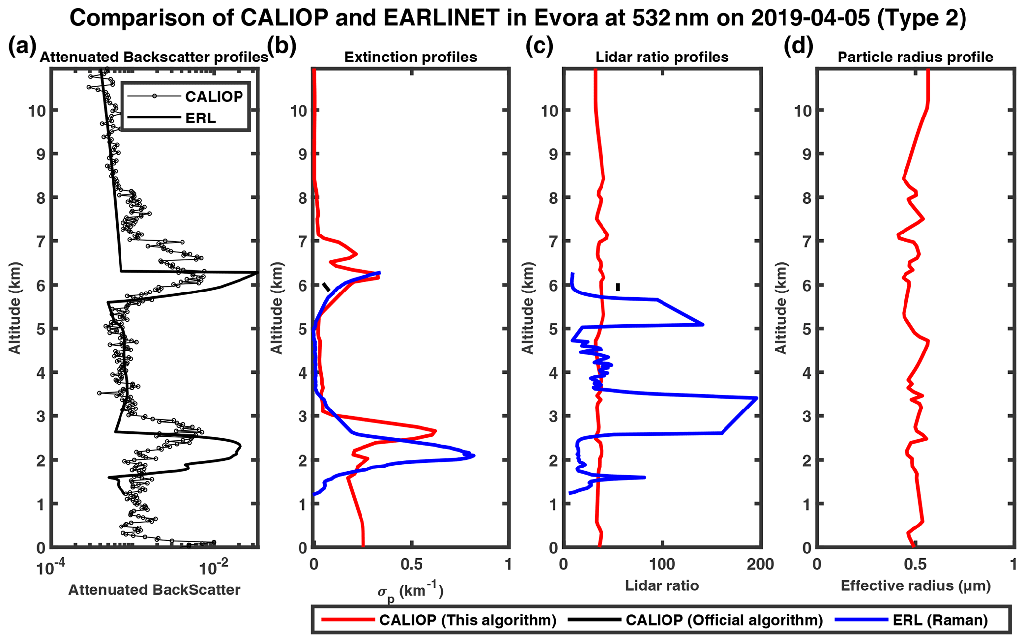
Figure 15The 532 and 1064 nm attenuated backscatter profiles measured by CALIOP (solid black line with circle marker) and the Evora Raman lidar (ERL) at the Evora station (remodeling, solid black line) on 20 August 2006 in a logarithmic scale in the horizontal direction (a); panels (b), (c) and (d) show the extinction profiles, lidar ratio profiles and particle radius profiles, respectively, provided by the modified inversion algorithm (red), CALIOP level 2 (black) and EARLINET level 2 (blue).
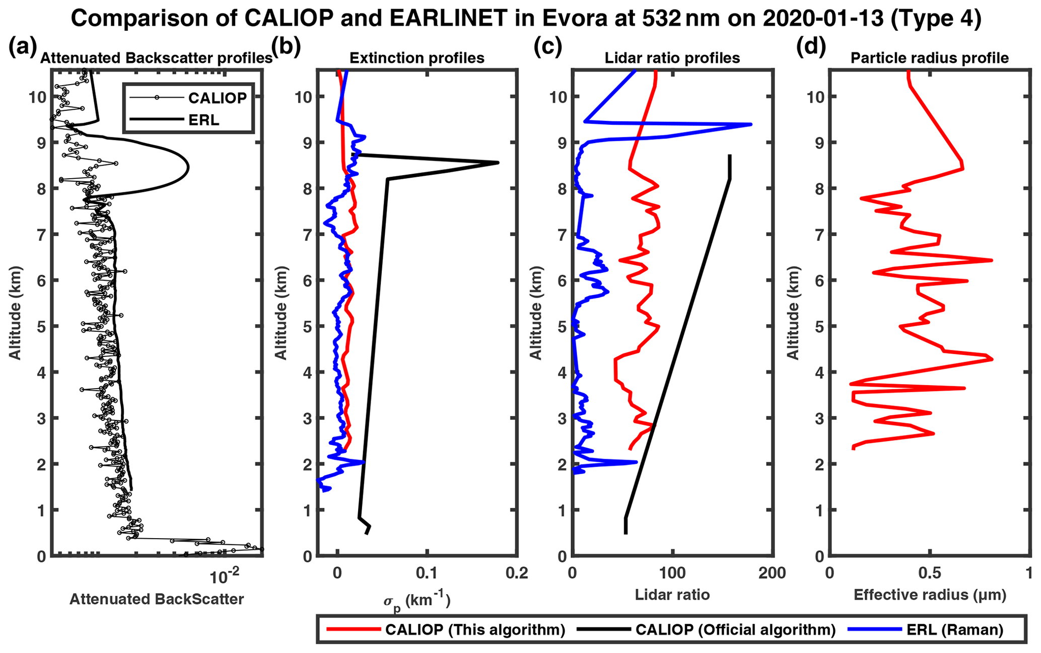
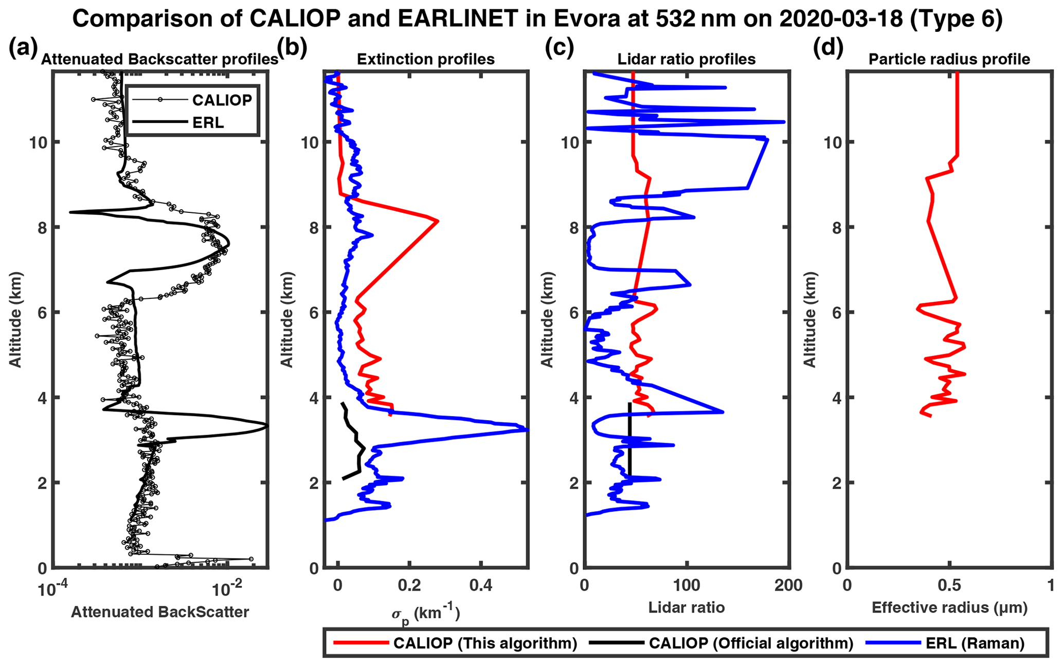
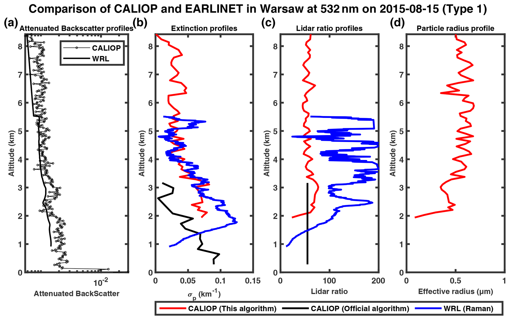
Figure 18The 532 and 1064 nm attenuated backscatter profiles measured by CALIOP (solid black line with circle marker) and the Warsaw Raman lidar (WRL) at the Warsaw station (remodeling, solid black line) on 20 August 2006 in a logarithmic scale in the horizontal direction (a); panels (b), (c) and (d) show the extinction profiles, lidar ratio profiles and particle radius profiles, respectively, provided by the modified inversion algorithm (red), CALIOP level 2 (black) and EARLINET level 2 (blue).
Uncertainties in aerosol extinction and effective radius profiles retrieved by our two-wavelength inversion algorithm are mainly due to measurement noise (e.g., the signal statistical error, the estimations of molecular optical properties), calibration errors and assumption errors. In this section, we further examine the errors associated with the assumptions in the algorithm.
First, the single-scattering approximation is used in solving the lidar equation, as multiple-scattering effects in aerosol layers are generally small and are currently neglected for CALIOP (Winker et al., 2009). We limit the application of our algorithm to clear-sky weather conditions to reduce this error, but this error is very difficult to quantify.
Second, the errors in the aerosol refractive index, size distribution and sphericity assumptions in lookup tables can also introduce errors into solving the lidar equation. The lognormal distribution assumption of the aerosol volume size distribution may make the algorithm fail to converge in other actual size distributions. For example, using data generated by a Junge distribution (a simpler aerosol size distribution), the algorithm cannot yield valid retrieval results. A similar outcome is noted for non-spherical particles or aerosol types significantly different from the assumed type.
Finally, we consider assumption and retrieval uncertainties to be a perturbation in the lidar ratio and attempt to quantify their effect on the retrieved profiles. We increase the lidar ratio profiles at 532 and 1064 nm from the lookup tables by ±10 % before calculating the synthetic attenuated backscatter profiles, which means the synthetic data do not entirely match the lookup table. The retrieval profiles exhibit mean MAPE of less than 14 % (in the 10 % case) and 17 % (in the −10 % case), indicating that the algorithm is comparatively robust to noise.
In this study, we described a modified lidar inversion algorithm to retrieve the aerosol extinction and size distribution simultaneously from two-wavelength elastic lidar measurements. Its major advantage over the operational CALIOP algorithm is that the lidar ratio of each layer is determined iteratively by the lidar ratio–AE lookup table. The algorithm was applied to the ground-based Raman lidar measurements at the PKU site, as well as to CALIOP measurements. The comparison results indicate that the retrieved aerosol extinction coefficient profiles using our method with CALIOP attenuated backscatter measurements are in good agreement with Raman lidar measurements. Characteristics of aerosol effective radius profiles are also retrieved, which can be used as a reference for aerosol size information.
In comparison with the iterative method by transcendental equations (Ackermann, 1997, 1998), our inversion uses lookup tables to simplify the complex calculation. Cao et al. (2019) develop a lidar ratio iteration method to invert the particle size distribution with an assumed Junge distribution, but the method was just used in simple simulation without actual tests. Although Lu et al. (2011) invert the aerosol backscatter coefficient profiles from CALIPSO lidar measurements by the iterative method, they failed to consider the size distribution of aerosols, which may have introduced uncertainties into the inversion. Compared with other modified CALIOP inversions by combining other measurements, such as ground-based lidar (Wang et al., 2007), our inversion is weaker because of the space–time limitations.
Additionally, this study still bears certain other limitations. The current algorithm is primarily suitable for fine-mode spherical particles, such as those that cause urban pollution, and considers the change of aerosol size (and thus the lidar ratio) with altitude due to long-range transport, vertical mixing, hygroscopic growth, etc. Non-spherical particles such as dust will be explored in the next step, possibly by taking advantage of the depolarization ratio (Gialitaki et al., 2020; Kahnert et al., 2020; Luo et al., 2022; Luo et al., 2019) measurement that is not used here. Another drawback is that although the algorithm does not need to assume a lidar ratio, the complex refractive index still needs to be assumed. As discussed above, the lidar ratio is very sensitive to the imaginary part and an incorrect assumption may induce errors or even makes the algorithm unable to converge. Therefore, this algorithm is mostly suitable when there is no significant change in aerosol type vertically. Finally, the polarization channel of CALIOP may contain additional aerosol type information but is only used when determining the initial refractive index (excluding dust) here. We also plan to refine our lookup table by incorporating polarization in order to improve the accuracy of the retrieval.
All raw data can be provided by the corresponding author upon request.
LC and JL planned the research; LC, JL, JR, CX and LZ developed the algorithm; LC and JL analyzed the results; LC and JL wrote the manuscript.
The contact author has declared that none of the authors has any competing interests.
Publisher’s note: Copernicus Publications remains neutral with regard to jurisdictional claims made in the text, published maps, institutional affiliations, or any other geographical representation in this paper. While Copernicus Publications makes every effort to include appropriate place names, the final responsibility lies with the authors.
This study is funded by the National Key Research and Development Program of China (grant no. 2023YFF0805401) and National Natural Science Foundation of China (NSFC) (grant no. 42175144).
This research has been supported by the National Key Research and Development Program of China (grant no. 2023YFF0805401) and the National Natural Science Foundation of China (grant no. 42175144).
This paper was edited by Meng Gao and reviewed by Zhongwei Huang and two anonymous referees.
Ackermann, J.: Two-wavelength lidar inversion algorithm for a two-component atmosphere, Appl. Opt., 36, 5134–5143, https://doi.org/10.1364/AO.36.005134, 1997.
Ackermann, J.: Two-wavelength lidar inversion algorithm for a two-component atmosphere with variable extinction-to-backscatter ratios, Appl. Opt., 37, 3164–3171, https://doi.org/10.1364/AO.37.003164, 1998.
Ansmann, A., Riebesell, M., and Weitkamp, C.: Measurement of atmospheric aerosol extinction profiles with a Raman lidar, Opt. Lett., 15, 746–748, https://doi.org/10.1364/OL.15.000746, 1990.
Bodhaine, B. A., Wood, N. B., Dutton, E. G., and Slusser, J. R.: On Rayleigh Optical Depth Calculations, J. Atmos. Ocean. Technol., 16, 1854–1861, https://doi.org/10.1175/1520-0426(1999)016<1854:orodc>2.0.co;2, 1999.
Burton, S. P., Ferrare, R. A., Hostetler, C. A., Hair, J. W., Rogers, R. R., Obland, M. D., Butler, C. F., Cook, A. L., Harper, D. B., and Froyd, K. D.: Aerosol classification using airborne High Spectral Resolution Lidar measurements – methodology and examples, Atmos. Meas. Tech., 5, 73–98, https://doi.org/10.5194/amt-5-73-2012, 2012.
Cai, Z., Li, Z., Li, P., Li, J., Sun, H., Yang, Y., Gao, X., Ren, G., Ren, R., and Wei, J.: Vertical distributions of aerosol microphysical and optical properties based on aircraft measurements made over the Loess Plateau in China, Atmos. Environ., 270, 118888, https://doi.org/10.1016/j.atmosenv.2021.118888, 2022.
Cao, N., Yang, S., Cao, S., Yang, S., and Shen, J.: Accuracy calculation for lidar ratio and aerosol size distribution by dual-wavelength lidar, Appl. Phys. A, 125, 590, https://doi.org/10.1007/s00339-019-2819-y, 2019.
Deshler, T., Hervig, M. E., Hofmann, D. J., Rosen, J. M., and Liley, J. B.: Thirty years of in situ stratospheric aerosol size distribution measurements from Laramie, Wyoming (41° N), using balloon-borne instruments, J. Geophys. Res.-Atmos., 108, 4167, https://doi.org/10.1029/2002jd002514, 2003.
Di Girolamo, P., De Rosa, B., Summa, D., Franco, N., and Veselovskii, I.: Measurements of Aerosol Size and Microphysical Properties: A Comparison Between Raman Lidar and Airborne Sensors, J. Geophys. Res.-Atmos., 127, e2021JD036086, https://doi.org/10.1029/2021JD036086, 2022.
Eswaran, K., Satheesh, S. K., and Srinivasan, J.: Sensitivity of aerosol radiative forcing to various aerosol parameters over the Bay of Bengal, J. Earth Syst. Sci., 128, 170, https://doi.org/10.1007/s12040-019-1200-z, 2019.
Fernald, F. G.: Analysis of atmospheric lidar observations: some comments, Appl. Opt., 23, 652–653, https://doi.org/10.1364/AO.23.000652, 1984.
Gialitaki, A., Tsekeri, A., Amiridis, V., Ceolato, R., Paulien, L., Kampouri, A., Gkikas, A., Solomos, S., Marinou, E., Haarig, M., Baars, H., Ansmann, A., Lapyonok, T., Lopatin, A., Dubovik, O., Groß, S., Wirth, M., Tsichla, M., Tsikoudi, I., and Balis, D.: Is the near-spherical shape the “new black” for smoke?, Atmos. Chem. Phys., 20, 14005–14021, https://doi.org/10.5194/acp-20-14005-2020, 2020.
Goto, D., Nakajima, T., Takemura, T., and Sudo, K.: A study of uncertainties in the sulfate distribution and its radiative forcing associated with sulfur chemistry in a global aerosol model, Atmos. Chem. Phys., 11, 10889–10910, https://doi.org/10.5194/acp-11-10889-2011, 2011.
Hara, K., Nishita-Hara, C., Osada, K., Yabuki, M., and Yamanouchi, T.: Characterization of aerosol number size distributions and their effect on cloud properties at Syowa Station, Antarctica, Atmos. Chem. Phys., 21, 12155–12172, https://doi.org/10.5194/acp-21-12155-2021, 2021.
He, Q., Li, C., Geng, F., Zhou, G., Gao, W., Yu, W., Li, Z., and Du, M.: A parameterization scheme of aerosol vertical distribution for surface-level visibility retrieval from satellite remote sensing, Remote Sens. Environ., 181, 1–13, https://doi.org/10.1016/j.rse.2016.03.016, 2016.
Hostetler, C., Liu, Z., Reagan, J., Vaughan, M., Winker, D., Osborn, M., Hunt, W., Powell, K., and Trepte, C.: CALIOP algorithm theoretical basis document calibration and Level 1 data products, Hampton, VA: NASA Langley Research Center, 26–29, https://www-calipso.larc.nasa.gov/resources/pdfs/PC-SCI-201v1.0.pdf (last access: 16 April 2024), 2006.
IPCC: Climate Change 2021 – The Physical Science Basis: Working Group I Contribution to the Sixth Assessment Report of the Intergovernmental Panel on Climate Change, Cambridge University Press, Cambridge, 35–115, https://doi.org/10.1017/9781009157896, 2023.
Kahnert, M., Kanngießer, F., Järvinen, E., and Schnaiter, M.: Aerosol-optics model for the backscatter depolarisation ratio of mineral dust particles, J. Quant. Spectrosc. Ra., 254, 107177, https://doi.org/10.1016/j.jqsrt.2020.107177, 2020.
Klett, J. D.: Lidar inversion with variable backscatter/extinction ratios, Appl. Opt., 24, 1638–1643, https://doi.org/10.1364/AO.24.001638, 1985.
Kudo, R., Nishizawa, T., and Aoyagi, T.: Vertical profiles of aerosol optical properties and the solar heating rate estimated by combining sky radiometer and lidar measurements, Atmos. Meas. Tech., 9, 3223–3243, https://doi.org/10.5194/amt-9-3223-2016, 2016.
Li, Y., Guo, X., Jin, L., Li, P., Sun, H., Zhao, D., and Ma, X.: Aircraft Measurements of Summer Vertical Distributions of Aerosols and Transitions to Cloud Condensation Nuclei and Cloud Droplets in Central Northern China, Chin. J. Atmos. Sci., 46, 845, https://doi.org/10.3878/j.issn.1006-9895.2104.20255, 2022.
Liu, P., Zhao, C., Zhang, Q., Deng, Z., Huang, M., Ma, X., and Tie, X.: Aircraft study of aerosol vertical distributions over Beijing and their optical properties, Tellus B, 61, 756–767, https://doi.org/10.1111/j.1600-0889.2009.00440.x, 2009.
Lu, X., Jiang, Y., Zhang, X., Wang, X., and Spinelli, N.: Two-wavelength lidar inversion algorithm for determination of aerosol extinction-to-backscatter ratio and its application to CALIPSO lidar measurements, J. Quant. Spectrosc. Ra., 112, 320–328, https://doi.org/10.1016/j.jqsrt.20doi:10.07.013, 2011.
Luo, J., Zhang, Q., Luo, J., Liu, J., Huo, Y., and Zhang, Y.: Optical Modeling of Black Carbon With Different Coating Materials: The Effect of Coating Configurations, J. Geophys. Res.-Atmos., 124, 13230–13253, https://doi.org/10.1029/2019JD031701, 2019.
Luo, J., Li, Z., Fan, C., Xu, H., Zhang, Y., Hou, W., Qie, L., Gu, H., Zhu, M., Li, Y., and Li, K.: The polarimetric characteristics of dust with irregular shapes: evaluation of the spheroid model for single particles, Atmos. Meas. Tech., 15, 2767–2789, https://doi.org/10.5194/amt-15-2767-2022, 2022.
Matthias, V., Freudenthaler, V., Amodeo, A., Balin, I., Balis, D., Bosenberg, J., Chaikovsky, A., Chourdakis, G., Comeron, A., Delaval, A., De Tomasi, F., Eixmann, R., Hagard, A., Komguem, L., Kreipl, S., Matthey, R., Rizi, V., Rodrigues, J., Wandinger, U., and Wang, X.: Aerosol lidar intercomparison in the framework of the EARLINET project. 1. Instruments, Appl. Opt., 43, 961–976, https://doi.org/10.1364/ao.43.000961, 2004.
Mishchenko, M. I. and Yang, P.: Far-field Lorenz–Mie scattering in an absorbing host medium: Theoretical formalism and FORTRAN program, J. Quant. Spectrosc. Ra., 205, 241–252, https://doi.org/10.1016/j.jqsrt.2017.doi:10.014, 2018.
National Geophysical Data, C.: U.S. standard atmosphere (1976), Planet. Space Sci., 40, 553–554, https://doi.org/10.1016/0032-0633(92)90203-Z, 1992.
Potter, J. F.: Two-frequency lidar inversion technique, Appl. Opt., 26, 1250–1256, https://doi.org/10.1364/AO.26.001250, 1987.
Rajeev, K. and Parameswaran, K.: Iterative method for the inversion of multiwavelength lidar signals to determine aerosol size distribution, Appl. Opt., 37, 4690–4700, https://doi.org/10.1364/AO.37.004690, 1998.
Tao, Z., McCormick, M. P., and Wu, D.: A comparison method for spaceborne and ground-based lidar and its application to the CALIPSO lidar, Appl. Phys. B, 91, 639, https://doi.org/10.1007/s00340-008-3043-1, 2008.
Veselovskii, I., Kolgotin, A., Griaznov, V., Müller, D., Wandinger, U., and Whiteman, D. N.: Inversion with regularization for the retrieval of tropospheric aerosol parameters from multiwavelength lidar sounding, Appl. Opt., 41, 3685–3699, https://doi.org/10.1364/AO.41.003685, 2002.
Wang, X., Frontoso, M. G., Pisani, G., and Spinelli, N.: Retrieval of atmospheric particles optical properties by combining ground-based and spaceborne lidar elastic scattering profiles, Opt. Express, 15, 6734–6743, https://doi.org/10.1364/OE.15.006734, 2007.
Winker, D. M., Vaughan, M. A., Omar, A., Hu, Y., Powell, K. A., Liu, Z., Hunt, W. H., and Young, S. A.: Overview of the CALIPSO Mission and CALIOP Data Processing Algorithms, J. Atmos. Ocean. Technol., 26, 2310–2323, https://doi.org/10.1175/2009jtecha1281.1, 2009.
Yang, J., Li, J., Li, P., Sun, G., Cai, Z., Yang, X., Cui, C., Dong, X., Xi, B., Wan, R., Wang, B., and Zhou, Z.: Spatial Distribution and Impacts of Aerosols on Clouds Under Meiyu Frontal Weather Background Over Central China Based on Aircraft Observations, J. Geophys. Res.-Atmos., 125, e2019JD031915, https://doi.org/10.1029/2019JD031915, 2020.
Zhang, L., Li, J., Jiang, Z., Dong, Y., Ying, T., and Zhang, Z.: Clear-Sky Direct Aerosol Radiative Forcing Uncertainty Associated with Aerosol Optical Properties Based on CMIP6 Models, J. Climate, 35, 3007–3019, https://doi.org/10.1175/JCLI-D-21-0479.1, 2022.
Zhang, Q., Ma, X., Tie, X., Huang, M., and Zhao, C.: Vertical distributions of aerosols under different weather conditions: Analysis of in-situ aircraft measurements in Beijing, China, Atmos. Environ., 43, 5526–5535, https://doi.org/10.1016/j.atmosenv.2009.05.037, 2009.